A microscopic theory of Curzon-Ahlborn heat engine

Abstract

The Curzon-Ahlborn (CA) efficiency, as the efficiency at the maximum power (EMP) of the endoreversible Carnot engine, has a significant impact on finite-time thermodynamics. However, the CA engine model is based on many assumptions. In the past few decades, although a lot of efforts have been made, a microscopic theory of the CA engine is still lacking. By adopting the method of the stochastic differential equation of energy, we formulate a microscopic theory of the CA engine realized with an underdamped Brownian particle in a class of non-harmonic potentials. This theory gives microscopic interpretation of all assumptions made by Curzon and Ahlborn, and thus puts the results about CA engine on a solid foundation. Also, based on this theory, we obtain analytical expressions of the power and the efficiency statistics for the Brownian CA engine. Our research brings new perspectives to experimental studies of finite-time microscopic heat engines featured with fluctuations.

Introduction.—For practical heat engines, not only the efficiency but also the power characterizes the performance. Optimizing the power and the efficiency of heat-engine cycles is one of the goals in the study of finite-time thermodynamics (Andresen, 2011; Berry et al., 2020). Compared to the Carnot efficiency achieved in infinite time (Callen, 1985), the efficiency at the maximum power (EMP) attracts a lot of attention in the studies of finite-time heat engines. The early studies (Yvon, 1955; Chambadal, 1957; Novikov, 1958; Curzon and Ahlborn, 1975; Rubin, 1979a; Moreau and Pomeau, 2015; Ouerdane et al., 2015; Feidt, 2017) of the endoreversible Carnot engine concluded that the EMP is the well-known Curzon-Ahlborn (CA) efficiency

$$\eta_{CA}=1-\sqrt{\frac{T_{C}}{T_{H}}},$$ (1)

where $T_{C}$ and $T_{H}$ denote the temperatures of the cold and the hot heat baths. The CA efficiency is in a similar form to the Carnot efficiency, and is only relevant to the temperatures of the two heat baths and is independent of any other characteristic of the heat engine. The CA efficiency aroused a lot of attention and led to many following-up researches (see for example Refs. (Rubin, 1979a, b; Schmiedl and Seifert, 2007a; Dechant et al., 2017)). It has become a paradigmatic result in studies dealing with thermodynamic optimization in the framework of finite-time and stochastic thermodynamics. In addition, the CA efficiency is relevant to many practical thermal machines (Esposito et al., 2010).

The CA efficiency as the EMP has also been derived in some different setups (Calvo Hernández et al., 2014). For example, in Ref. (Van den Broeck, 2005) it is shown that CA efficiency is a result which can be obtained in the well-founded linear irreversible thermodynamics. In Ref. (Esposito et al., 2010), the CA efficiency, as the EMP, is derived in the symmetric low-dissipation regime, where the irreversible entropy production is assumed inversely proportional to the period of a cycle. Such a $1/\tau$-scaling has been recently verified in the experiment of finite-time isothermal compression of dry air (Ma et al., 2020a; Chen et al., 2021). These studies confirm the validity of the CA efficiency as the EMP in many heat engine models. Meanwhile, in some other models, the EMP deviates from the CA efficiency (Van den Broeck, 2005; Schmiedl and Seifert, 2007a; Tu, 2008; Izumida and Okuda, 2008; Esposito et al., 2010; Wang and He, 2012; Cavina et al., 2017; Ma et al., 2018a; Abiuso and Perarnau-Llobet, 2020; Abah et al., 2012; de Cisneros and Hernández, 2007; Izumida and Okuda, 2009; Sánchez-Salas et al., 2010; Nakamura et al., 2020; Fu et al., 2020; Lavenda, 2007; Tu, 2020; Bauer et al., 2016; Chen, 1994; Chen et al., 2019; Dann et al., 2020; Deffner, 2018; Smith et al., 2020; Bonança, 2019; Tu, 2012; Chen et al., 2011), probably due to different circumstances of these models.

The original derivation of the CA efficiency (Yvon, 1955; Chambadal, 1957; Novikov, 1958; Curzon and Ahlborn, 1975) is based on a lot of assumptions, such as the endoreversible assumption and the assumption of constant temperature difference. But how reliable are those assumptions made by Curzon and Ahlborn remains unclarified due to the lack of a microscopic theory of the CA engine. Also, due to this lack, the control scheme of the work parameter which is essential to construct the optimal cycle can not be determined (except for the harmonic potential (Dechant et al., 2017)), neither can the work and heat statistics as well as the fluctuation theorems of the CA engine. In the past few decades, a lot of efforts have been made to seek a microscopic interpretation of the CA engine, but were unsuccessful.

In this Letter, we fill this long-standing gap by realizing the CA engine with an underdamped Brownian particle (Hondou and Sekimoto, 2000; Blickle and Bechinger, 2011; Martínez et al., 2015; Holubec and Marathe, 2020; Gieseler et al., 2014; Gong et al., 2016; Kwon et al., 2013; Dechant et al., 2017; Gomez-Marin et al., 2008; Celani et al., 2012) in a time-dependent potential as the working substance. By adopting the method of stochastic differential equation of energy (Salazar and Lira, 2016, 2019), we give microscopic interpretation of all assumptions made by Curzon and Ahlborn, including the endoreversibility, Newton’s cooling law and the constant temperature difference. Thus we lay a solid foundation for the CA engine model. Furthermore, this microscopic theory allows us to determine the control scheme of the work parameter of the Brownian CA engine and study the fluctuations of the power and the efficiency of the Brownian CA engine. Our study demonstrates that when downsizing the working substance to a single Brownian particle, results about the average power and efficiency of the CA engine remain valid, but the fluctuations become prominent.

The model.—The working substance of the engine is modeled as a Brownian particle (Jun et al., 2014; Gieseler et al., 2014; Martínez et al., 2015, 2016, 2017; Hoang et al., 2018; Albay et al., 2020; Tu, 2014; Li et al., 2017; Li and Tu, 2019; Paneru et al., 2018; Speck, 2011; Schmiedl and Seifert, 2007b; Rana et al., 2014) constrained in a controllable potential $\mathcal{U}(x,t)=k(t)x^{2n}/(2n)$ with the control parameter $k(t)$ and a positive integer $n$. In the isothermal expansion (compression) process, the control parameter $k(t)$ is varied when the engine is in contact with the heat bath at temperature $T_{\mathrm{b}}$. The motion of the particle with mass $m$ is governed by the complete Langevin equation

$$\ddot{x}+\gamma\dot{x}+k(t)x^{2n-1}=\frac{1}{m}\xi(t),$$ (2)

where the random force $\xi(t)$ represents a Gaussian white noise satisfying $\langle\xi(t)\rangle=0$ and $\langle\xi(t)\xi(t^{\prime})\rangle=2m\gamma T_{\mathrm{b}}\delta(t-t^{\prime})$ with the friction coefficient $\gamma$. Throughout the text the Boltzmann constant is set to be $k_{B}=1$.

We consider the highly underdamped regime $\tau_{p}\ll\gamma^{-1}$ and slow external driving $\tau_{p}\ll k/\dot{k}$, where $\tau_{p}$ is the period of the unperturbed motion of the particle, e.g., $\tau_{p}=2\pi\sqrt{m/k}$ for a harmonic oscillator ($n=1$). Under these two conditions, the variation of the stochastic energy of the particle within a period is relatively small, which allows us to study the dynamics of the stochastic energy $E=m\dot{x}^{2}/2+\mathcal{U}(x,t)$. Based on Ito’s lemma and Virial theorem, the equation of motion is expressed as the stochastic differential equation of the energy $E$ (Salazar and Lira, 2016, 2019)

$$dE=\frac{\dot{\lambda}}{\lambda}Edt-\Gamma\left(E-\frac{f_{n}T_{\mathrm{b}}}{2}\right)dt+\sqrt{2\Gamma T_{\mathrm{b}}E}dB_{t}.$$ (3)

where the work parameter is rewritten into $\lambda(t)=k(t)^{1/(n+1)}$ with the increment $dB_{t}$ of the Wiener process, the effective friction coefficient $\Gamma=2n\gamma/(n+1)$, and the effective degrees of freedom $f_{n}=1+1/n$. The increment of trajectory work for this system is

$$dW=\frac{\dot{\lambda}}{\lambda}Edt.$$ (4)

The trajectory heat is obtained from the first law of thermodynamics as

$$dQ=-\Gamma\left(E-\frac{f_{n}T_{\mathrm{b}}}{2}\right)dt+\sqrt{2\Gamma T_{\mathrm{b}}E}dB_{t}.$$ (5)

The Fokker-Planck equation associated with Eq. (3) can be solved explicitly (Salazar and Lira, 2019). During the dynamical evolution process, the system remains in a Maxwell-Boltzmann distribution in the energy space and thus can be described by an effective temperature $\theta(t)$ as

$$P(E,t)=\frac{e^{-E/\theta(t)}}{\Gamma(f_{n}/2)}\frac{E^{f_{n}/2-1}}{\theta(t)^{f_{n}/2}},$$ (6)

where $\Gamma(x)=\int_{0}^{\infty}e^{-y}y^{x-1}dy$ is gamma function. Notice that Eq. (6) leads to the endoreversibility, which is usually assumed in previous studies relevant to the CA engine, but is derived as a consequence of the equation of motion in our setup. The ensemble average of the energy is $\langle E(t)\rangle=f_{n}\theta(t)/2$ with the effective temperature $\theta(t)$ governed by

$$\dot{\theta}(t)=\frac{\dot{\lambda}}{\text{$\lambda$}}\theta(t)-\Gamma[\theta(t)-T_{\mathrm{b}}].$$ (7)

We emphasize that the l.h.s. of Eq. (7) corresponds to the time derivative of the average energy up to a factor $f_{n}/2$. The two terms on the r.h.s. correspond to the average work flux and heat flux, respectively. The average heat flux satisfies Newton’s cooling law, which is also derived as a consequence of the equation of motion. The effective friction coefficient $\Gamma$, as a cooling rate, is independent of the work parameter $\lambda$. We would like to point out that a similar equation of motion for the effective temperature $\theta(t)$ has been obtained previously for the ideal gas as the working substance (Rubin, 1979b). However, their derivation relies on several assumptions, for example, the equation of state of ideal gas, the phenomenological Newton’s cooling law and the endoreversible assumption. On the contrary, the results presented here are all derived from the microscopic dynamics, and are capable of describing microscopic systems featured with fluctuations.

Realization of Curzon-Ahlborn engine based on a Brownian particle.—With the model introduced above, we study the EMP of such a microscopic Brownian engine and formulate a microscopic theory of the CA engine. To construct a finite-time Carnot cycle, two heat baths at different temperatures $T_{i},\>i=H,C$ are required in the hot and the cold isothermal processes. The (effective) friction coefficients $\gamma_{i}$ ($\Gamma_{i}$) may be different in the two processes. Based on Curzon and Ahlborn’s derivation (Curzon and Ahlborn, 1975), we summarize the preconditions of the CA engine as follows

1. Endoreversibility (Hoffmann et al., 1997). The state of the working substance of the engine can be described by an effective temperature.

2. Newton’s cooling law (or linear heat transfer law). The heat flux between the working substance and the heat bath is proportional to the temperature difference.

3. Constant temperature difference. During the isothermal expansion (compression) process, the effective temperature of the working substance remains at a constant value $\theta_{H}\>(\theta_{C})$ different from that of the heat bath $T_{H}\,(T_{C})$.

4. Internal reversible Carnot cycle. All irreversibilities are associated with the heat exchange between the working substance and the heat baths while the adiabatic processes remain reversible (Calvo Hernández et al., 2014). The heat engine operates like a reversible Carnot engine between two virtual heat baths at temperatures $\theta_{C}$ and $\theta_{H}$, respectively.

5. Constant heat capacity (Johal and Jayannavar, 2021) and cooling rate (Apertet et al., 2017). Both the heat capacity of the working substance and the cooling rate are independent of the temperature and the work parameters.

According to Eqs. (6) and (7), our setup fulfills requirements (i) and (ii). In supplementary material, we prove that the optimal cycle corresponding to the maximum power is exactly the CA cycle satisfying preconditions (iii) and (iv). Precondition (v) is guaranteed by the generalized equipartition theorem and the highly underdamped condition.

Based on the equation of motion of the effective temperature (Eq. (7)) and the definition of trajectory work and heat, we can optimize the average power of the finite-time Brownian engine. In Fig. 1(a), we plot the cycle diagram of the Brownian CA engine. In order to construct a closed CA cycle, the values of work parameter at the end of each process in Fig. 1(a) satisfy

$$\frac{\lambda_{2}}{\lambda_{1}}=\frac{\lambda_{3}}{\lambda_{4}}=r.$$ (8)

The four processes of the CA cycle are illustrated as follows (see supplementary material),

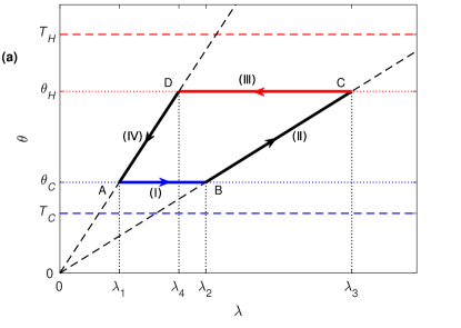
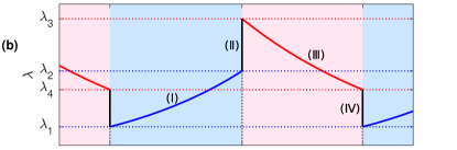
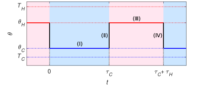
Figure 1: CA cycle based on a Brownian particle. (a) The cycle diagram in the space of the work parameter $\lambda$ and the effective temperature $\theta$. In the isothermal expansion (compression) process, the working substance remains at a constant effective temperature $\theta_{H}(\theta_{C})$, which is different from the temperature $T_{H}(T_{C})$ of the hot (cold) heat bath. In the two adiabatic processes, the effective temperature $\theta$ of the working substance is proportional to the work parameter $\lambda$. (b) The control scheme of the work parameter $\lambda(t)$ and the evolution of the effective temperature $\theta(t)$ in a finite-time cycle. The work parameter $\lambda$ is varied exponentially with time in an isothermal process, and is quenched abruptly in an adiabatic process.

1. Isothermal compression. The working substance is in contact with the cold heat bath. Initiated from $\lambda_{1}$ at $t=0$, the work parameter is varied exponentially with time $\lambda(t)=\lambda_{1}(\lambda_{2}/\lambda_{1})^{t/\tau_{C}}$, where $\tau_{C}$ is the duration of the process. From the protocol, it can be found that the effective temperature of the working substance remains at a constant during the process

   $$\theta_{C}=\frac{\tau_{C}\Gamma_{C}}{\tau_{C}\Gamma_{C}-\ln r}T_{C}.$$ (9)

   The heat released to the cold heat bath during the isothermal compression process is

   $$-\left\langle Q_{C}\right\rangle=\frac{f_{n}}{2}\Gamma_{C}(\theta_{C}-T_{C})\tau_{C}.$$ (10)

2. Adiabatic compression. The work parameter $\lambda(t)$ is quenched instantaneously from $\lambda_{2}$ to $\lambda_{3}$ with the effective temperature $\theta(t)$ changing from $\theta_{C}$ to $\theta_{H}$ accordingly. When the timescale of varying the work parameter is much shorter than that of the heat dissipation, Eq. (7) becomes $\dot{\theta}(t)=\dot{\lambda}\theta(t)/\lambda$, which leads to $\theta_{H}/\theta_{C}=\lambda_{3}/\lambda_{2}$.

3. Isothermal expansion. The working substance is in contact with the hot heat bath. The work parameter is varied exponentially with time $\lambda(t)=\lambda_{3}(\lambda_{4}/\lambda_{3})^{(t-\tau_{C})/\tau_{H}}$, and the working substance remains at a constant effective temperature

   $$\theta_{H}=\frac{\tau_{H}\Gamma_{H}}{\tau_{H}\Gamma_{H}+\ln r}T_{H},$$ (11)

   where $\tau_{H}$ is the duration of the process. The heat absorbed from the hot heat bath during the isothermal expansion process is

   $$\left\langle Q_{H}\right\rangle=\frac{f_{n}}{2}\Gamma_{H}(T_{H}-\theta_{H})\tau_{H}.$$ (12)

4. Adiabatic expansion. Finally, the work parameter is quenched from $\lambda_{4}$ to the initial value $\lambda_{1}$ instantaneously with the effective temperature changing from $\theta_{H}$ to $\theta_{C}$ accordingly, satisfying $\theta_{H}/\theta_{C}=\lambda_{4}/\lambda_{1}$.

The control scheme of the work parameter $\lambda$ and the evolution of the effective temperature $\theta$ in a finite-time cycle are illustrated in Fig. 1(b).

Combing Eqs. (9)-(12), it is straightforward to verify the precondition (iv) that the entropy change of the working substance after a cycle is zero $\Delta S=\left\langle Q_{H}\right\rangle/\theta_{H}+\left\langle Q_{C}\right\rangle/\theta_{C}=0.$ Therefore, the microscopic dynamics of the model, together with the explicit control scheme $\lambda(t)$, constitutes a microscopic theory of the CA engine.

The net work of a full cycle is $-\left\langle W\right\rangle=\left\langle Q_{H}\right\rangle+\left\langle Q_{C}\right\rangle$, and the average power and the average efficiency follow as $\overline{P}\coloneqq-\left\langle W\right\rangle/(\tau_{H}+\tau_{C})$ and $\eta\coloneqq-\left\langle W\right\rangle/\left\langle Q_{H}\right\rangle$, which are explicitly

$$\overline{P}=\frac{f_{n}\ln r}{2(\tau_{H}+\tau_{C})}\left(\frac{\tau_{H}\Gamma_{H}T_{H}}{\tau_{H}\Gamma_{H}+\ln r}-\frac{\tau_{C}\Gamma_{C}T_{C}}{\tau_{C}\Gamma_{C}-\ln r}\right),$$ (13)

and

$$\eta=1-\frac{1+(\tau_{H}\Gamma_{H})^{-1}\ln r}{1-(\tau_{C}\Gamma_{C})^{-1}\ln r}\frac{T_{C}}{T_{H}}.$$ (14)

In order to achieve the maximum power, we first fix $r$ and optimize the power over $\tau_{H}$ and $\tau_{C}$. The maximum power is obtained as (see supplementary material)

$$\overline{P}_{\mathrm{max}}=\frac{f_{n}\Gamma_{C}\Gamma_{H}\left(\sqrt{T_{H}}-\sqrt{T_{C}}\right)^{2}}{2\left(\sqrt{\Gamma_{H}}+\sqrt{\Gamma_{C}}\right)^{2}},$$ (15)

with the corresponding optimal duration of the two isothermal processes

$$\tau_{H}^{\mathrm{max}}=\frac{\ln r\left(\sqrt{\Gamma_{H}T_{H}}+\sqrt{\Gamma_{C}T_{C}}\right)}{\Gamma_{H}\sqrt{\Gamma_{C}}\left(\sqrt{T_{H}}-\sqrt{T_{C}}\right)},$$

$$\tau_{C}^{\mathrm{max}}=\frac{\ln r\left(\sqrt{\Gamma_{H}T_{H}}+\sqrt{\Gamma_{C}T_{C}}\right)}{\Gamma_{C}\sqrt{\Gamma_{H}}\left(\sqrt{T_{H}}-\sqrt{T_{C}}\right)}.$$ (16)

Please note that $\overline{P}_{\mathrm{max}}$ is independent of $r$. Hence $\overline{P}_{\mathrm{max}}$ is also the global maximum power. It is straightforward to see that the EMP of the Brownian engine in the highly underdamped regime is the CA efficiency

$$\eta_{\mathrm{EMP}}=1-\sqrt{\frac{T_{C}}{T_{H}}}=\eta_{CA},$$ (17)

as we expect. Based on Eqs. (14) and (15), we derive the trade-off relation between power and efficiency in supplementary material. Compared to previous studies (Shiraishi et al., 2016; Holubec and Ryabov, 2016; Gonzalez-Ayala et al., 2017; Pietzonka and Seifert, 2018; Ma et al., 2018b; Abiuso and Perarnau-Llobet, 2020), our trade-off relation is tight and is shown to be reachable with the explicit control scheme of the work parameter $\lambda(t)$. It is worth mentioning that Ref. (Chen and Yan, 1989) obtains the same tight trade-off relation, and Ref. (Dechant et al., 2017) obtains the tight trade-off relation as well as the control scheme for the harmonic potential. As a generalization, our results are valid for a Brownian particle in a class of non-harmonic potentials.

Generating function of work and heat in a finite-time isothermal process.—For a microscopic Brownian engine, average values are insufficient to characterize the performance. Fluctuations are non-negligible (Holubec and Ryabov, 2021). To evaluate the performance of a finite-time heat engine, we need to quantify the extracted work and heat absorbed from the hot bath in one heat-engine cycle. For the dynamics described by the above model, we can derive the analytical results of the joint generating function of work and heat $I(u,s)\coloneqq\left\langle e^{uQ+sW}\right\rangle$ by generalizing the techniques used in Ref. (Salazar, 2020). The result is

$$I(u,s)=\left[\frac{1+u\tilde{\psi}(\tau)}{1+u\tilde{\psi}_{0}}\right]^{\frac{f_{n}}{2}}e^{\frac{f_{n}(s-u)}{2}\int_{0}^{\tau}\frac{\dot{\lambda}(t)}{\lambda(t)}\psi(t)dt},$$ (18)

where $\tau$ is the time duration of the process, and the temperature-like variable $\psi(t)$ satisfies

$$\frac{d\psi}{dt}=\frac{\dot{\lambda}}{\text{$\lambda$}}\psi-\Gamma(\psi-T_{\mathrm{b}})+(s-u)\frac{\dot{\lambda}}{\lambda}\psi^{2}.$$ (19)

with the initial condition $\psi(0)=\tilde{\psi}_{0}/(1+u\tilde{\psi}_{0})$. The initial value $\tilde{\psi}_{0}$ is either set as the initial temperature $\theta_{0}$ or obtained from the previous process. A shifted temperature-like variable is defined as $\tilde{\psi}(t)\coloneqq\psi(t)/[1-u\psi(t)]$, whose value $\tilde{\psi}(\tau)$ at the end of this process is used as the initial value $\tilde{\psi}_{0}$ of the subsequent process. Detailed derivations to Eqs. (18) and (19) and the analytical expression of the joint generating function $I(u,s)$ are left in supplementary material.

Statistics of power and efficiency of the Brownian CA engine.—Based on the microscopic theory, especially the joint generating function of work and heat $I(u,s)$ and the control scheme $\lambda(t)$ of the full cycle, we can further study the fluctuations of the power and the efficiency (Holubec, 2014; Denzler and Lutz, 2021a, 2020, b; Holubec and Ryabov, 2021; Salazar, 2020) together with the fluctuation theorems (Sinitsyn, 2011; Seifert, 2012) of the finite-time Brownian Carnot engine. Specifically, we calculate the distribution $p(P)$ of the fluctuating power $P\coloneqq-W/(\tau_{C}+\tau_{H})$ and the distribution $p(\zeta)$ of the fluctuating efficiency $\zeta\coloneqq-(W+\eta Q_{H})/\left\langle Q_{H}\right\rangle$ from the generating function $I_{\mathrm{cycle}}(u_{H},u_{C},s)=\left\langle e^{u_{H}Q_{H}+u_{C}Q_{C}+sW}\right\rangle$ (see supplementary material) of a whole cycle. Please note that, instead of $-W/Q_{H}$, we define $\zeta$ as the fluctuating efficiency which characterizes the deviation from the average efficiency $\eta$ defined above. It is straightforward to see that $\left\langle\zeta\right\rangle=0$.

As a special case, we plot the distributions of the power and the efficiency of the Brownian CA engine in Fig. 2, where $\eta=\eta_{CA}$, $\tau_{C}=\tau_{C}^{\mathrm{max}}$, $\tau_{H}=\tau_{H}^{\mathrm{max}}$. Due to the fluctuation, the power can be negative or much larger than the average power. Similarly, the efficiency can be negative or larger than Carnot efficiency (even larger than unity). From the analytical results of the joint generating function $I_{\mathrm{cycle}}(u_{H},u_{C},s)$, we can show the tendency of the distributions when we increase the duration of the cycle $\tau_{\mathrm{t}}\coloneqq\tau_{C}^{\mathrm{max}}+\tau_{H}^{\mathrm{max}}$ by increasing $\ln r$

$$\mathrm{Var}(P) \approx\frac{4\overline{P}_{\mathrm{max}}^{2}}{f_{n}\eta_{CA}^{2}}\frac{\left[(1-\eta_{CA})^{2}+1/\delta\right]\left(1+\delta\right)}{\sqrt{\Gamma_{C}\Gamma_{H}}}\frac{1}{\tau_{\mathrm{t}}},$$ (20)

$$\mathrm{Var}(\zeta) \approx\frac{4(1-\eta_{CA})^{2}}{f_{n}\sqrt{\Gamma_{C}\Gamma_{H}}}\frac{(1+\delta)^{2}}{\delta}\frac{1}{\tau_{\mathrm{t}}},$$ (21)

where $\delta=\sqrt{\Gamma_{H}T_{H}/(\Gamma_{C}T_{C})}$. For both the power and the efficiency, their variances decrease inversely with $\tau_{\mathrm{t}}$.

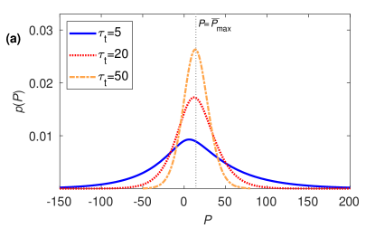
Figure 2: Distribution of the power (a) and the efficiency (b) of a Brownian CA engine for three different periods $\tau_{\mathrm{t}}=5,\,20,\,50$. (a) The vertical dotted line indicates the average power. (b) The vertical solid, dashed and dotted lines correspond to efficiency $\eta=0$, $\eta=\eta_{C}$ (Carnot efficiency) and $\eta=1$ respectively. Here we have chosen $T_{C}=300$, $T_{H}=600$, $\Gamma_{C}=1$, $\Gamma_{H}=1.2$.

Summary and discussion.—In this Letter, we realize the Curzon-Ahlborn heat engine with a Brownian particle in the highly underdamped regime. By adopting the method of stochastic differential equation of energy, we formulate a microscopic theory of the CA engine based on this model. This theory gives microscopic interpretation of all assumptions of the CA engine model including the endoreversibility, Newton’s cooling law and the constant temperature difference. Hence, we lay a solid foundation for the CA engine.

From this microscopic theory, the explicit control scheme $\lambda(t)$ of the CA engine can be uniquely determined, which leads to the maximum power of the Brownian engine. The control scheme associated with the maximum power for any given efficiency can be obtained based on the microscopic theory. In addition, we calculate the generating function of work and heat, and obtain the analytical results of statistics of the power and the efficiency together with the fluctuation theorems of the Brownian CA engine. These quantitative results about the CA engine bring important insights to the studies of finite-time thermodynamics beyond the low-dissipation regime (Esposito et al., 2010; Holubec and Ryabov, 2016; Gonzalez-Ayala et al., 2017; Ma et al., 2018b; Gonzalez-Ayala et al., 2020; Abiuso and Perarnau-Llobet, 2020; Ma et al., 2020b). For example, results about the average power and efficiency of the CA engine remain valid when downsizing the working substance to a single Brownian particle, but fluctuations become prominent. Our study will shed new light on the experimental explorations about finite-time Brownian engine, and may inspire future studies about the design of nanomachines with higher power and efficiency.

Acknowledgement.—H. T. Quan thanks Zhan-Chun Tu for valuable comments and acknowledges support from the National Science Foundation of China under Grants No. 11775001, No. 11534002, and No. 11825001.

References

- Andresen (2011) B. Andresen, Angew. Chem. Int. Ed. 50, 2690 (2011).
- Berry et al. (2020) R. Berry, P. Salamon, and B. Andresen, Entropy 22, 908 (2020).
- Callen (1985) H. Callen, Thermodynamics and an introduction to thermostatistics (Wiley, New York, 1985).
- Yvon (1955) J. Yvon, in First Geneva Conf. Proc. UN (1955).
- Chambadal (1957) P. Chambadal, Les Centrales Nuclaires (Armand Colin, France, 1957).
- Novikov (1958) I. Novikov, J. Nucl. Eng. 7, 125 (1958).
- Curzon and Ahlborn (1975) F. L. Curzon and B. Ahlborn, Am. J. Phys 43, 22 (1975).
- Rubin (1979a) M. H. Rubin, Phys. Rev. A 19, 1272 (1979a).
- Moreau and Pomeau (2015) M. Moreau and Y. Pomeau, Eur. Phys. J. Special Topics 224, 769 (2015).
- Ouerdane et al. (2015) H. Ouerdane, Y. Apertet, C. Goupil, and P. Lecoeur, Eur. Phys. J. Special Topics 224, 839 (2015).
- Feidt (2017) M. Feidt, Entropy 19, 369 (2017).
- Rubin (1979b) M. H. Rubin, Phys. Rev. A 19, 1277 (1979b).
- Schmiedl and Seifert (2007a) T. Schmiedl and U. Seifert, EPL (Europhysics Letters) 81, 20003 (2007a).
- Dechant et al. (2017) A. Dechant, N. Kiesel, and E. Lutz, Europhys. Lett. 119, 50003 (2017).
- Esposito et al. (2010) M. Esposito, R. Kawai, K. Lindenberg, and C. V. Broeck, Phys. Rev. Lett. 105, 150603 (2010).
- Calvo Hernández et al. (2014) A. Calvo Hernández, J. Roco, A. Medina, and N. Sánchez-Salas, Rev. Mex. Fís. 60, 384 (2014).
- Van den Broeck (2005) C. Van den Broeck, Phys. Rev. Lett. 95, 190602 (2005).
- Ma et al. (2020a) Y.-H. Ma, R.-X. Zhai, J. Chen, C. P. Sun, and H. Dong, Phys. Rev. Lett. 125, 210601 (2020a).
- Chen et al. (2021) J.-F. Chen, C. P. Sun, and H. Dong, Phys. Rev. E 104, 034117 (2021).
- Tu (2008) Z. C. Tu, J. Phys. A: Math. Theor. 41, 312003 (2008).
- Izumida and Okuda (2008) Y. Izumida and K. Okuda, Europhys. Lett. 83, 60003 (2008).
- Wang and He (2012) J. Wang and J. He, Phys. Rev. E 86, 051112 (2012).
- Cavina et al. (2017) V. Cavina, A. Mari, and V. Giovannetti, Phys. Rev. Lett. 119, 050601 (2017).
- Ma et al. (2018a) Y.-H. Ma, D. Xu, H. Dong, and C.-P. Sun, Phys. Rev. E 98, 022133 (2018a).
- Abiuso and Perarnau-Llobet (2020) P. Abiuso and M. Perarnau-Llobet, Phys. Rev. Lett. 124, 110606 (2020).
- Abah et al. (2012) O. Abah, J. Roßnagel, G. Jacob, S. Deffner, F. Schmidt-Kaler, K. Singer, and E. Lutz, Phys. Rev. Lett. 109, 203006 (2012).
- de Cisneros and Hernández (2007) B. J. de Cisneros and A. C. Hernández, Phys. Rev. Lett. 98, 130602 (2007).
- Izumida and Okuda (2009) Y. Izumida and K. Okuda, Phys. Rev. E 80, 021121 (2009).
- Sánchez-Salas et al. (2010) N. Sánchez-Salas, L. López-Palacios, S. Velasco, and A. C. Hernández, Phys. Rev. E 82, 051101 (2010).
- Nakamura et al. (2020) K. Nakamura, J. Matrasulov, and Y. Izumida, Phys. Rev. E 102, 012129 (2020).
- Fu et al. (2020) R. Fu, A. Taghvaei, Y. Chen, and T. T. Georgiou, (2020), arXiv:2001.00979 [math.OC] .
- Lavenda (2007) B. H. Lavenda, Am. J. Phys. 75, 169 (2007).
- Tu (2020) Z.-C. Tu, Front. Phys. 16, 33202 (2020).
- Bauer et al. (2016) M. Bauer, K. Brandner, and U. Seifert, Phys. Rev. E 93, 042112 (2016).
- Chen (1994) J. Chen, J. Phys. D: Appl. Phys. 27, 1144 (1994).
- Chen et al. (2019) J.-F. Chen, C.-P. Sun, and H. Dong, Phys. Rev. E 100, 062140 (2019).
- Dann et al. (2020) R. Dann, R. Kosloff, and P. Salamon, Entropy 22, 1255 (2020).
- Deffner (2018) S. Deffner, Entropy 20, 875 (2018).
- Smith et al. (2020) Z. Smith, P. S. Pal, and S. Deffner, J. Non-Equilib. Thermodyn. 45, 305 (2020).
- Bonança (2019) M. V. S. Bonança, J. Stat. Mech.: Theory Exp. 2019, 123203 (2019).
- Tu (2012) Z.-C. Tu, Chin. Phys. B 21, 020513 (2012).
- Chen et al. (2011) L. Chen, Z. Ding, and F. Sun, J. Non-Equilib. Thermodyn. 36, 155 (2011).
- Hondou and Sekimoto (2000) T. Hondou and K. Sekimoto, Phys. Rev. E 62, 6021 (2000).
- Blickle and Bechinger (2011) V. Blickle and C. Bechinger, Nat. Phys. 8, 143 (2011).
- Martínez et al. (2015) I. A. Martínez, É. Roldán, L. Dinis, D. Petrov, J. M. R. Parrondo, and R. A. Rica, Nat. Phys. 12, 67 (2015).
- Holubec and Marathe (2020) V. Holubec and R. Marathe, Phys. Rev. E 102, 060101 (2020).
- Gieseler et al. (2014) J. Gieseler, R. Quidant, C. Dellago, and L. Novotny, Nat. Nanotechnology 9, 358 (2014).
- Gong et al. (2016) Z. Gong, Y. Lan, and H. Quan, Phys. Rev. Lett. 117, 180603 (2016).
- Kwon et al. (2013) C. Kwon, J. D. Noh, and H. Park, Phys. Rev. E 88, 062102 (2013).
- Gomez-Marin et al. (2008) A. Gomez-Marin, T. Schmiedl, and U. Seifert, J. Chem. Phys. 129, 024114 (2008).
- Celani et al. (2012) A. Celani, S. Bo, R. Eichhorn, and E. Aurell, Phys. Rev. Lett. 109, 260603 (2012).
- Salazar and Lira (2016) D. S. P. Salazar and S. A. Lira, J. Phys. A: Math. Theor. 49, 465001 (2016).
- Salazar and Lira (2019) D. S. P. Salazar and S. A. Lira, Phys. Rev. E 99, 062119 (2019).
- Jun et al. (2014) Y. Jun, M. Gavrilov, and J. Bechhoefer, Phys. Rev. Lett. 113, 190601 (2014).
- Martínez et al. (2016) I. A. Martínez, A. Petrosyan, D. Guéry-Odelin, E. Trizac, and S. Ciliberto, Nat. Phys. 12, 843 (2016).
- Martínez et al. (2017) I. A. Martínez, É. Roldán, L. Dinis, and R. A. Rica, Soft Matter 13, 22 (2017).
- Hoang et al. (2018) T. M. Hoang, R. Pan, J. Ahn, J. Bang, H. Quan, and T. Li, Phys. Rev. Lett. 120, 080602 (2018).
- Albay et al. (2020) J. A. C. Albay, P.-Y. Lai, and Y. Jun, Appl. Phys. Lett. 116, 103706 (2020).
- Tu (2014) Z. C. Tu, Phys. Rev. E 89, 052148 (2014).
- Li et al. (2017) G. Li, H. T. Quan, and Z. C. Tu, Phys. Rev. E 96, 012144 (2017).
- Li and Tu (2019) G. Li and Z. C. Tu, Phys. Rev. E 100, 012127 (2019).
- Paneru et al. (2018) G. Paneru, D. Y. Lee, T. Tlusty, and H. K. Pak, Phys. Rev. Lett. 120, 020601 (2018).
- Speck (2011) T. Speck, J. Phys. A: Math. Theor. 44, 305001 (2011).
- Schmiedl and Seifert (2007b) T. Schmiedl and U. Seifert, Phys. Rev. Lett. 98, 108301 (2007b).
- Rana et al. (2014) S. Rana, P. Pal, A. Saha, and A. Jayannavar, Phys. Rev. E 90, 042146 (2014).
- Hoffmann et al. (1997) K. H. Hoffmann, J. M. Burzler, and S. Schubert, J. Non-Equilib. Thermodyn. 22, 311 (1997).
- Johal and Jayannavar (2021) R. S. Johal and A. M. Jayannavar, Resonance 26, 211 (2021).
- Apertet et al. (2017) Y. Apertet, H. Ouerdane, C. Goupil, and P. Lecoeur, Phys. Rev. E 96, 022119 (2017).
- Shiraishi et al. (2016) N. Shiraishi, K. Saito, and H. Tasaki, Phys. Rev. Lett. 117, 190601 (2016).
- Holubec and Ryabov (2016) V. Holubec and A. Ryabov, J. Stat. Mech: Theory Exp. 2016, 073204 (2016).
- Gonzalez-Ayala et al. (2017) J. Gonzalez-Ayala, A. C. Hernández, and J. M. M. Roco, Phys. Rev. E 95, 022131 (2017).
- Pietzonka and Seifert (2018) P. Pietzonka and U. Seifert, Phys. Rev. Lett. 120, 190602 (2018).
- Ma et al. (2018b) Y.-H. Ma, D. Xu, H. Dong, and C.-P. Sun, Phys. Rev. E 98, 042112 (2018b).
- Chen and Yan (1989) L. Chen and Z. Yan, J. Chem. Phys. 90, 3740 (1989).
- Holubec and Ryabov (2021) V. Holubec and A. Ryabov, (2021), arXiv:2108.00172 [cond-mat.stat-mech] .
- Salazar (2020) D. S. P. Salazar, Phys. Rev. E 101, 030101 (2020).
- Holubec (2014) V. Holubec, J. Stat. Mech.: Theory Exp. 2014, P05022 (2014).
- Denzler and Lutz (2021a) T. Denzler and E. Lutz, New J. Phys. 23, 075003 (2021a).
- Denzler and Lutz (2020) T. Denzler and E. Lutz, Phys. Rev. Research 2, 032062 (2020).
- Denzler and Lutz (2021b) T. Denzler and E. Lutz, Phys. Rev. Research 3, L032041 (2021b).
- Sinitsyn (2011) N. Sinitsyn, J. Phys. A: Math. Theor. 44, 405001 (2011).
- Seifert (2012) U. Seifert, Rep. Prog. Phys. 75, 126001 (2012).
- Gonzalez-Ayala et al. (2020) J. Gonzalez-Ayala, J. Guo, A. Medina, J. Roco, and A. C. Hernández, Phys. Rev. Lett. 124, 050603 (2020).
- Ma et al. (2020b) Y.-H. Ma, C. P. Sun, and H. Dong, (2020b), arXiv:2012.08748 [quant-ph] .