Noisy Channel Language Model Prompting
for Few-Shot Text Classification

Abstract

We introduce a noisy channel approach for language model prompting in few-shot text classification. Instead of computing the likelihood of the label given the input (referred as direct models), channel models compute the conditional probability of the input given the label, and are thereby required to explain every word in the input. We use channel models for recently proposed few-shot learning methods with no or very limited updates to the language model parameters, via either in-context demonstration or prompt tuning. Our experiments show that, for both methods, channel models significantly outperform their direct counterparts, which we attribute to their stability, i.e., lower variance and higher worst-case accuracy. We also present extensive ablations that provide recommendations for when to use channel prompt tuning instead of other competitive methods (e.g., direct head tuning): channel prompt tuning is preferred when the number of training examples is small, labels in the training data are imbalanced, or generalization to unseen labels is required.

1 Introduction

Prompting large language models, by prepending natural language text or continuous vectors (called prompts) to the input, has shown to be promising in few-shot learning (Brown et al., 2020). Prior work has proposed methods for finding better prompt  (Shin et al., 2020; Li and Liang, 2021; Lester et al., 2021) or better scoring of the output from the model (Zhao et al., 2021; Holtzman et al., 2021). These studies directly predict target tokens to determine the prediction for an end task. Despite promising results, they can be unstable with high variance across different verbalizers (text expression for labels) and seeds, and the worst-case performance is often close to random (Perez et al., 2021; Lu et al., 2021).

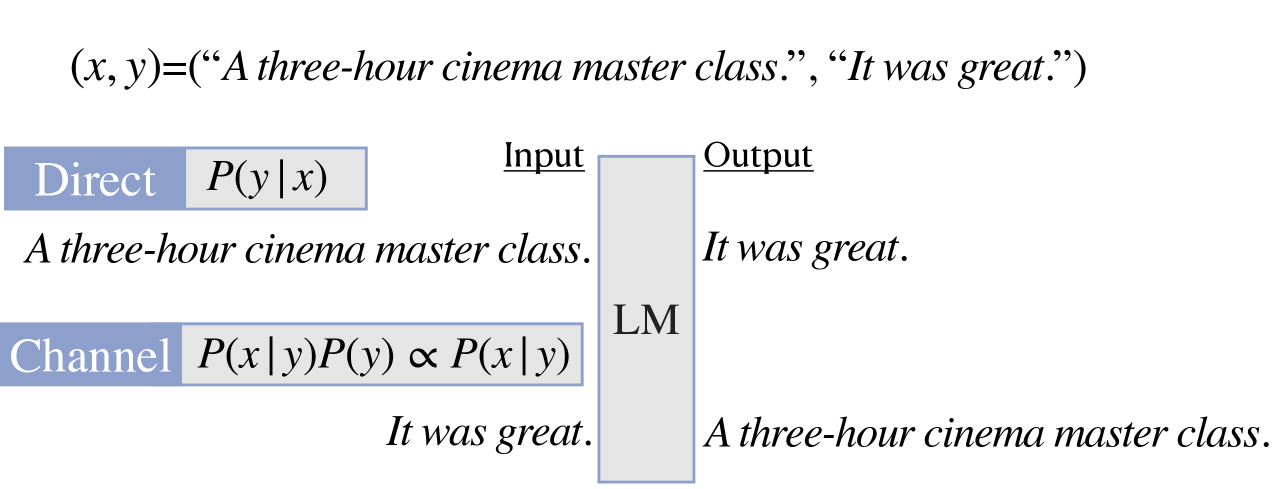
Figure 1: An illustration of the direct model and the channel model for language model prompting in the sentiment analysis task.

In this paper, we introduce alternative channel models for prompted few-shot text classification with large language models, inspired by noisy channel models in machine translation (Brown et al., 1993; Koehn et al., 2003; Yu et al., 2017; Yee et al., 2019) and their extensions to other tasks (Yogatama et al., 2017; Lewis and Fan, 2018). Unlike direct models that compute the conditional probability of the label token given the input, channel models compute the conditional probability of the input given the output (Figure 1). Intuitively, channel models are required to explain every word in the input, potentially amplifying training signals in the low data regime. We study the impact of channel models for language model prompting where the parameters of the language model are frozen. In particular, we compare channel models with their direct counterparts for (1) demonstration methods, either concatenation-based (Brown et al., 2020) or our proposed, ensemble-based (Section 4.1.3), and (2) prompt tuning (Lester et al., 2021).

Our experiments on eleven text classification datasets show that channel models outperform their direct counterparts by a large margin. We attribute the strong performance of channel models to their stability: they have lower variance and significantly higher worst-case accuracy then their direct counterparts over different verbalizers and seeds. We additionally find a direct model with head tuning—tuning the LM head while freezing other parameters—is surprisingly effective, often outperforming direct models with other forms of tuning. While different methods are preferred given different conditions, the channel model with prompt tuning (denoted as channel prompt tuning) significantly outperforms all direct baselines when (1) the training data is imbalanced, or (2) generalization to unseen labels is required.

In summary, our contributions are three-fold:

1. We introduce a noisy channel approach for language model prompting in few-shot text classification, showing that they significantly outperform their direct counterparts for both demonstration methods and prompt tuning.

2. We find particularly strong performance of channel models over direct models when the training data is imbalanced or generalization to unseen labels is required.

3. Based on extensive ablations, we provide recommendations between different models (direct vs. channel and prompt tuning vs. head tuning) based on given conditions such as the target task, the size of training data, the number of classes, the balance between labels in the training data, and whether generalization to unseen labels is required.

2 Related Work

2.1 Channel Model

Let $x$ and $y$ be the input and the output, respectively. The most widely used models, denoted as direct models, compute $P(y|x)$. In contrast, noisy channel models maximize $P(x|y)P(y)$ (Shannon, 1948; Brown et al., 1993). While the noisy channel approach has been the most successful in machine translation (Yamada and Knight, 2001; Koehn et al., 2003; Yu et al., 2017; Yee et al., 2019), it has also been studied in more general NLP tasks. Prior work provides a theoretical analysis that channel models approach their asymptotic errors more rapidly than their direct counterparts (Ng and Jordan, 2002), and empirically shows that channel models are more robust to distribution shift in text classification (Yogatama et al., 2017) or question answering (Lewis and Fan, 2018), and in a few-shot setup (Ding and Gimpel, 2019).

In this paper, we explore channel models using a large language model on a wide range of text classification tasks, focusing on prompt-based few-shot learning.

2.2 Few-shot Learning

Prior work in few-shot learning has used different approaches, including semi-supervised learning with data augmentation or consistency training (Miyato et al., 2017; Clark et al., 2018; Xie et al., 2020; Chen et al., 2020) and meta learning (Finn et al., 2017; Huang et al., 2018; Bansal et al., 2020). Recent work has introduced prompting (or priming) of a large language model. For example, Brown et al. (2020) proposes to use a concatenation of training examples as a demonstration, so that when it is prepended to the input and is fed to the model, the model returns the output following the pattern in the training examples. This is especially attractive as it eliminates the need for updating parameters of the language model, which is often expensive and impractical. Subsequent work proposes alternative ways of scoring labels through better model calibration (Zhao et al., 2021; Holtzman et al., 2021), or learning better prompts, either in a discrete space (Shin et al., 2020; Jiang et al., 2020; Gao et al., 2021) or in a continuous space (Li and Liang, 2021; Lester et al., 2021; Liu et al., 2021; Zhong et al., 2021; Qin and Eisner, 2021). Almost all of them are direct models, computing the likelihood of $y$ given $x$ with the prompts.

Our work is closely related to two recent papers. Tam et al. (2021) studies a label-conditioning objective for masked language models; although this is not strictly a generative channel model, conditioning on the output $y$ is similar to our work. However, they are still optimizing a discriminative objective, and inference at test time is the same as with the direct model. Holtzman et al. (2021) explores zero-shot models that compute the probability of $x$ given $y$ based on Pointwise Mutual Information, but with a restriction that the input and the output are interchangeable. To the best of our knowledge, our work is the first that uses a noisy channel model for few-shot language model prompting for classification, and also the first to draw the connection with the noisy channel literature.

3 Formulation

Method	Zero-shot	Concat-based Demonstrations	Ensemble-based Demonstrations
Direct	$P_{\mathrm{LM}}(v(c_{i})|x)$	$P_{\mathrm{LM}}(v(c_{i})|x^{1},v(c^{1})...x^{k},v(c^{k}),x)$	$\Pi_{j=1}^{K}P_{\mathrm{LM}}(v(c_{i})|x^{j},v(c^{j}),x)$
Direct++	$\frac{P_{\mathrm{LM}}(v(c_{i})|x)}{P_{\mathrm{LM}}(v(c_{i})|\texttt{NULL})}$	$\frac{P_{\mathrm{LM}}(v(c_{i})|x^{1},v(c^{1})...x^{k},v(c^{k}),x)}{P_{\mathrm{LM}}(v(c_{i})|x^{1},v(c^{1})...x^{k},v(c^{k}),\texttt{NULL})}$	$\Pi_{j=1}^{K}\frac{P_{\mathrm{LM}}(v(c_{i})|x^{j},v(c^{j}),x)}{P_{\mathrm{LM}}(v(c_{i})|x^{j},v(c^{j}),\texttt{NULL})}$
Channel	$P_{\mathrm{LM}}(x|v(c_{i}))$	$P_{\mathrm{LM}}(x|x^{1},v(c^{1})...x^{k},v(c^{k}),v(c_{i}))$	$\Pi_{j=1}^{K}P_{\mathrm{LM}}(x|v(c^{j}),x^{j},v(c_{i}))$

Table 1: Comparison of zero-shot, concat-based demonstrations, and ensemble-based demonstrations (Section 4.1). $\{(x^{j},c^{j})\}_{j=1}^{K}$ is training data and $v$ is the verbalizer.

We focus on text classification tasks. The goal is to learn a task function $f:\mathcal{X}\xrightarrow{}\mathcal{C}$, where $\mathcal{X}$ is the set of all natural language texts and $\mathcal{C}=\{c_{1}...c_{m}\}$ is a set of labels. We consider three formulations.

Direct computes distributions of labels $c_{i}\in\mathcal{C}$ given the input $x\in\mathcal{X}$: $P(c_{i}|x)$. This is the most widely used method in modern neural networks.

Direct++ is a stronger direct model that computes $\frac{P(c_{i}|x)}{P(c_{i}|\texttt{NULL})}$ instead of $P(c_{i}|x)$, following the method from Holtzman et al. (2021) and the non-parametric method from Zhao et al. (2021). This approach is motivated by the fact that language models can be poorly calibrated and suffer from competition between different strings with the same meaning. This approach is used for the demonstration methods in Section 4.1.

Channel uses Bayes’ rule to reparameterize $P(c_{i}|x)$ as $\frac{P(x|c_{i})P(c_{i})}{P(x)}$. As we are generally interested in $\mathrm{argmax}_{c_{i}\in\mathcal{C}}\frac{P(x|c_{i})P(c_{i})}{P(x)}$ and $P(x)$ is independent from $c_{i}$, it is sufficient to model $P(x|c_{i})P(c_{i})$. We assume $P(c_{i})=\frac{1}{|\mathcal{C}|}$ and only compute $P(x|c_{i})$.

4 Method

We explore direct and channel models using a causal language model (LM) $P_{\mathrm{LM}}$ that gives the conditional probability of the text $y$ when followed by $x$. More precisely, given the text $x=x_{1}...x_{t_{x}}$ and $y=y_{1}...y_{t_{y}}$ ($x_{1}...x_{t_{x}},y_{1}...y_{t_{y}}\in\mathcal{V}$, where $\mathcal{V}$ is the vocabulary set), $P_{\mathrm{LM}}(y|x)$ indicates $\Pi_{t^{\prime}=1}^{t_{y}}P_{\mathrm{LM}}(y_{t^{\prime}}|x_{1}...x_{t_{x}}y_{1}...y_{t^{\prime}-1})$.

When learning a task function $f:\mathcal{X}\xrightarrow{}\mathcal{C}$, we also assume a pre-defined verbalizer $v:\mathcal{C}\xrightarrow{}\mathcal{X}$ which maps each label into a natural language expression. For example, if the task is sentiment analysis with $\mathcal{C}=\{c^{+},c^{-}\}$, an example input text $x$ would be “A three-hour cinema master class” and an example $v$ would have $v(c^{+})=$“It was great” and $v(c^{-})=$“It was terrible”. In a few-shot setup, we are also given a set of $K$ training examples $\mathcal{D}=\{(x^{1},c^{1}),\cdots,(x^{K},c^{K})\}$.

We are interested in methods where there are no trainable parameters (Section 4.1) or the number of trainable parameters is very small, typically less than 0.01% of the total (Section 4.2). This follows prior observations that updating and saving a large number of parameters for every task is expensive and often infeasible (Rebuffi et al., 2017; Houlsby et al., 2019; Lester et al., 2021).

4.1 Demonstration methods

In demonstration methods, there are no trainable parameters. We explore three ways of making a prediction, as summarized in Table 1.

4.1.1 Zero-shot

We follow Brown et al. (2020) in computing $P(c_{i}|x)$ and $P(x|c_{i})$ as $P_{\mathrm{LM}}(v(c_{i})|x)$ and $P_{\mathrm{LM}}(x|v(c_{i}))$, respectively. For example, given $x=$“A three-hour cinema master class”, the direct model compares the probabilities of “It was great” and “It was terrible” when following “A three-hour cinema master class”, while the channel model considers the probabilities of “A three-hour cinema master class” when following “It was great” or “It was terrible”.

4.1.2 Concat-based demonstrations

We follow the few-shot learning method in Brown et al. (2020). The key idea is to prepend a concatenation of $K$ training examples to the input so that a language model can learn the task setup from the input. The original method was used for a direct model, but can be naturally extended for a channel model. Concretely, $P(c_{i}|x)$ in direct models is obtained via $P_{\mathrm{LM}}(v(c_{i})|x^{1},v(c^{1}),\cdots,x^{K},v(c^{K}),x)$, and $P(x|c_{i})$ in channel models is obtained via $P_{\mathrm{LM}}(x|v(c^{1}),x^{1},\cdots,v(c^{K}),x^{K},v(c_{i}))$.

4.1.3 Ensemble-based demonstrations

We propose a new method as an alternative to the concat-based method, which we find to be a stronger direct model. Instead of concatenating $K$ training examples as one sequence and getting output probabilities from an LM once, we obtain output probabilities from an LM $K$ times conditioned on one training example at a time, and multiply the resulting probabilities. Specifically, $P(c_{i}|x)$ is computed via $\Pi_{j=1}^{K}P_{\mathrm{LM}}(v(c_{i})|x^{j},v(c^{j}),x)$ and $P(x|c_{i})$ is computed via $\Pi_{j=1}^{K}P_{\mathrm{LM}}(x|v(c^{j}),x^{j},v(c_{i}))$. This method also reduces the memory consumption—the concat-based method uses $O(K^{2})$ while this method uses $O(K)$—and eliminates the dependency on the ordering of training examples, which has been shown to significantly impact the model performance (Zhao et al., 2021; Lu et al., 2021).

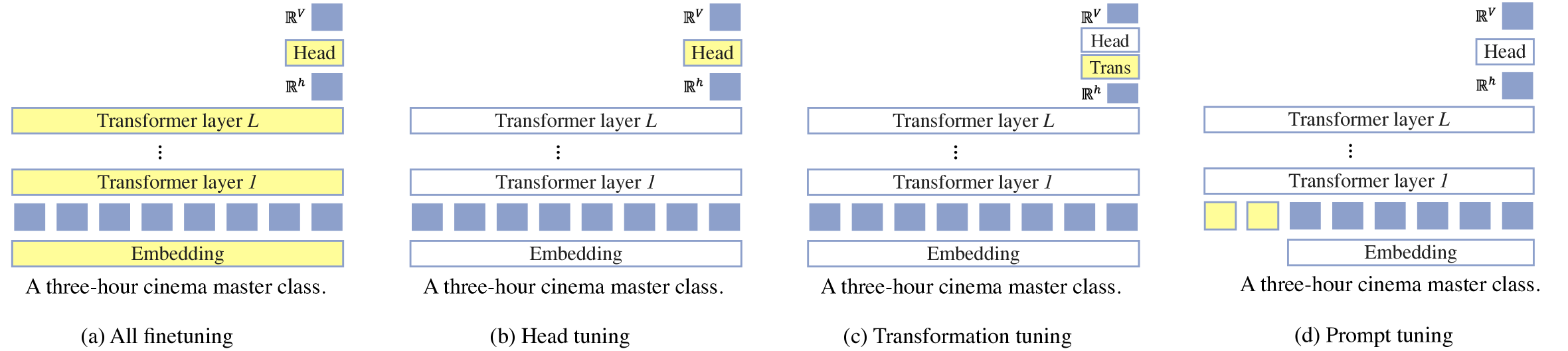
Figure 2: Different finetuning methods, which compute the distributions of the next token given “A three-hour cinema master class”. Yellow and white boxes are trainable and frozen parameters, respectively. $h$ and $V$ denote the hidden dimension of the LM and the vocabulary size of $v(c_{1})...v(c_{m})$, respectively. All finetuning is a typical finetuning method that updates all parameters of the LM (illustrated as a reference). Head tuning, Transformation tuning and Prompt tuning are described in Section 4.2; they update a very limited number of parameters.

4.2 Tuning methods

We also explore methods that tune a very limited number of model parameters, as summarized in Figure 2. We study head tuning (Section 4.2.1) and transformation tuning (Section 4.2.2) for direct models. We also consider prompt tuning (Section 4.2.3) for both direct and channel models, which we refer as direct prompt tuning and channel prompt tuning, respectively. All models share the same input-output interface with the zero-shot setup in Table 1 during training and inference.

4.2.1 Head tuning

Head tuning finetunes the head—the matrix in the LM which transforms the hidden representation from the last transformer layer to the logit values. Let $\mathbf{O}\in\mathbb{R}^{|\mathcal{V}|\times h}$ be the head and $\mathbf{h}_{x}\in\mathbb{R}^{h}$ be the hidden representations from the last transformer layer given $x$, $P_{\mathrm{LM}}(v_{i}|x)$ for a token $v_{i}\in\mathcal{V}$ is computed via an $i$-th element of $\mathrm{Softmax}(\mathbf{O}\mathbf{h}_{x})$. We finetune $\mathbf{O}$ while freezing all other parameters of the LM. Although $\mathbf{O}$ is tied with the embedding matrix of the LM during language model pretraining, we separate them during head tuning.

4.2.2 Transformation tuning

As an alternative to head tuning, we transform $\mathbf{O}$ with a new transformation matrix $\mathbf{U}\in\mathbb{R}^{h\times h}$. Specifically, $P_{\mathrm{LM}}(v_{i}|x)$ for a token $v_{i}\in\mathcal{V}$ is computed via an $i$-th element of $\mathrm{Softmax}(\mathbf{O}\mathbf{U}\mathbf{h}_{x})$. We train $\mathbf{U}$, initialized from an identity matrix, and freeze other parameters including $\mathbf{O}$.

4.2.3 Prompt tuning

Prompt tuning is the method that has recently gathered much attention (Li and Liang, 2021; Lester et al., 2021; Liu et al., 2021). The key idea is to consider the LM as a black-box model and instead learn continuous prompt embeddings. We follow the method from Lester et al. (2021) where $n$ prompt tokens $u_{1}...u_{n}$ are prepended to the input, and the embeddings of $u_{1}...u_{n}$ are learned. In other words, direct models compute $P(c_{i}|x)=P_{\mathrm{LM}}(v(c_{i})|u_{1}...u_{n},x)$, and channel models compute $P(x|c_{i})=P_{\mathrm{LM}}(x|u_{1}...u_{n},v(c_{i}))$. The parameters in the LM are frozen except the embeddings of $u_{1}...u_{n}$.

5 Experimental Setup

Dataset	Task	$|\mathcal{C}|$
SST-2	Sentiment analysis (movie)	2
SST-5	Sentiment analysis (movie)	5
MR	Sentiment analysis (movie)	2
CR	Sentiment analysis (electronics)	2
Amazon	Sentiment analysis (Amazon)	5
Yelp	Sentiment analysis (Yelp)	5
TREC	Question classification (answer type)	6
AGNews	News classification (topic)	4
Yahoo	Question classification (topic)	10
DBPedia	Ontology classification	14
Subj	Subjectivity classification	2

Table 2: Datasets used for experiments. $|\mathcal{C}|$ denotes the number of classes.See Appendix A for samples.

5.1 Datasets

We report results for eleven text classification datasets, following Zhang et al. (2015) and Gao et al. (2021): SST-2 (Socher et al., 2013), SST-5 (Socher et al., 2013), MR (Pang and Lee, 2005), CR (Hu and Liu, 2004), Amazon (McAuley and Leskovec, 2013), Yelp (Zhang et al., 2015), TREC (Voorhees and Tice, 2000), AGNews (Zhang et al., 2015), Yahoo (Zhang et al., 2015), DBPedia (Lehmann et al., 2015) and Subj (Pang and Lee, 2004). The datasets include a varied number of classes per task, from 2 to 14. See Table 10 in Appendix A for dataset samples.

Data	Zero-shot (4 runs)			Concat-based (20 runs)			Ensemble-based (20 runs)
	Direct	Direct++	Channel	Direct	Direct++	Channel	Direct	Direct++	Channel
SST-2	63.0/51.1	80.3/76.9	77.1/74.8	58.9/50.6	66.8/51.7	85.0/83.1	57.5/50.9	79.7/68.0	77.5/59.5
SST-5	27.5/24.4	33.3/28.8	29.2/27.7	27.6/23.0	23.7/14.4	36.2/32.7	25.6/23.2	33.8/23.3	33.6/30.2
MR	61.7/50.3	77.4/73.2	74.3/69.3	56.4/50.0	60.2/50.5	80.5/76.8	58.8/50.0	76.8/60.1	76.1/60.0
CR	59.2/50.0	77.9/69.7	65.8/60.2	54.7/50.0	66.8/50.0	80.8/74.8	51.0/50.0	72.8/54.6	79.7/69.3
Amazon	31.2/22.4	37.6/35.0	37.1/31.6	33.0/21.4	40.8/35.7	39.4/34.3	31.7/23.1	39.8/32.0	40.4/36.2
Yelp	33.2/25.6	36.8/31.8	38.0/31.9	32.6/23.3	38.5/31.6	39.8/36.5	31.4/23.6	39.2/29.6	41.5/38.5
AGNews	59.8/47.8	59.9/44.0	61.8/59.7	34.0/25.0	51.2/34.4	68.5/60.6	51.9/34.2	73.1/58.6	74.3/69.3
TREC	38.7/26.0	27.7/12.6	30.5/19.4	27.2/9.4	31.6/13.0	42.0/26.8	32.1/13.0	22.9/9.8	31.5/23.8
Yahoo	20.7/17.8	35.3/28.7	48.7/48.1	13.0/10.0	29.6/19.4	56.2/52.3	16.6/10.7	50.6/46.5	58.6/57.4
DBPedia	32.3/18.6	37.6/30.4	51.4/42.7	32.5/7.1	71.1/55.2	58.5/40.0	46.8/17.1	72.6/55.7	64.8/57.0
Subj	51.0/49.9	52.0/48.8	57.8/51.5	53.7/49.9	56.9/50.0	60.5/40.8	51.6/49.6	52.2/41.8	52.4/46.9
Avg.	43.5/34.9	50.5/43.6	52.0/47.0	38.5/29.1	48.8/36.9	58.9/50.8	41.4/31.4	55.8/43.6	57.3/49.8

Table 3: Results from demonstration methods. All with GPT-2 Large. Two numbers respectively indicate the average and the worst-case accuracy over different verbalizers (zero-shot and few-shot) and data seeds (few-shot). ‘Avg.’ in the last row indicate the macro-average across all datasets.

5.2 Training Data

For few-shot learning, we primarily use training set size $K=16$, but explore $K=\{4,16,64,\mathrm{Full}\}$ in the ablations. We sample the $K$ examples uniformly from the true distribution of the training data. We relax the assumption from prior work of an equal number of training examples per label (Gao et al., 2021; Logan IV et al., 2021), for more realistic and challenging evaluation.

We follow all the hyperameters and details from prior work (Appendix B) which eliminates the need for a held-out validation set. The very limited data is better used for training rather than validation, and cross-validation is less helpful when the validation set is extremely small (Perez et al., 2021).

5.3 Language Models

We use GPT-2 (Radford et al., 2019) for the LM. We primarily use GPT-2 Large but also experiment with varying sizes (Small, Medium, Large and X-Large) for the ablations in Appendix C. While we only experiment with GPT-2, our experiments are easily extendable to other causal language models.

5.4 Evaluation

We use accuracy as a metric for all datasets.

We experiment with 4 different verbalizers (taken from Gao et al. (2021); full list provided in Appendix A), 5 different random seeds for sampling training data, and 4 different random seeds for training. We then report Average accuracy and Worst-case accuracy. We consider the worst-case accuracy to be as important as the average accuracy given significantly high variance of few-shot learning models, as shown in previous work (Zhao et al., 2021; Perez et al., 2021). The worst-case accuracy is likely of more interest in high-risk applications (Asri et al., 2016; Guo et al., 2017).

Other implementation details are in Appendix B. All experiments are reproducible from github.com/shmsw25/Channel-LM-Prompting.

6 Experimental Results

This section reports results from demonstration methods (Section 6.1), tuning methods (Section 6.2) and ablations (Section 6.3). Discussion is provided in Section 7.

6.1 Main Results: Demonstration Methods

Table 3 shows the performance of demonstration methods.

Direct vs. Direct++

Direct++ significantly outperforms the naive direct model across all setups, indicating that using $\frac{P(c_{i}|x)}{P(c_{i}|\texttt{NULL})}$ instead of $P(c_{i}|x)$ is highly beneficial as claimed by Holtzman et al. (2021); Zhao et al. (2021).

Concat vs. Ensemble

Our proposed, ensemble-based method is better than the concat-based method in direct models, by 7% absolute in the average accuracy and the worst-case accuracy, when macro-averaged across all datasets.

In contrast, the ensemble-based method is not always better in channel models; it is better only on the datasets with long inputs. We conjecture that the ensemble-based method may suffer when labels in the training data are not balanced, which direct++ explicitly takes into account as described in Zhao et al. (2021).

Direct++ vs. Channel

In a few-shot setting, channel models outperform direct models in almost all cases. The strongest channel model outperforms the strongest direct model by 3.1% and 7.2% absolute, in terms of the average accuracy and the worst-case accuracy, respectively.

Standard deviation and the best-case accuracy are reported in Table 11 and Table 12 in the Appendix. They indicate strong performance of channel models can be attributed to their low variance. The highest best-case accuracy is achieved by direct++ on most datasets, but it has a higher variance, having lower average and the worst-case accuracy than channel models.

Zero-shot vs. Few-shot

Performance of direct models sometimes degrades in a few-shot setting, which is also observed by prior work (Zhao et al., 2021). This is likely because demonstrations provided by the training data may cause the model to be miscalibrated and easily biased by the choice of demonstrations. However, channel models achieve few-shot performance that is significantly better than zero-shot methods on all datasets.

6.2 Main Results: Tuning Methods

Table 4 shows the performance of tuning methods.

Comparison when prompt tuning

When using prompt tuning, channel models consistently outperform direct models by a large margin on all datasets. Improvements are 13.3% and 23.5% absolute in the average and the worst-case accuracy, respectively.

Standard deviation and the best-case accuracy are reported in Table 13 in the Appendix. Consistent with the findings in Section 6.1, the strong performance of channel prompt tuning can be explained by the low variance of channel prompt tuning. Direct prompt tuning often achieves higher best-case accuracy; however, due to its high variance, its overall accuracy is lower, with significantly lower worst-case accuracy.

Data	Direct			Channel
	Head	Trans	Prompt	Prompt
SST-2	80.2/68.6	77.3/57.5	72.6/50.9	85.8/81.3
SST-5	34.9/30.0	33.0/25.5	30.9/19.1	36.3/27.9
MR	73.7/56.4	71.3/51.6	67.4/50.1	81.7/78.0
CR	67.6/50.0	63.9/50.0	65.7/50.0	79.6/76.4
Amazon	34.5/28.8	32.1/18.2	31.2/20.0	43.4/39.2
Yelp	40.6/32.8	38.9/31.5	31.9/20.6	43.9/37.2
TREC	54.1/42.4	48.0/31.0	35.9/13.0	37.1/20.8
AGNews	74.1/61.2	66.9/47.0	61.9/25.2	73.4/63.9
Yahoo	39.1/31.4	33.8/23.0	27.4/15.7	54.0/46.7
DBPedia	49.3/37.5	42.4/28.6	41.8/9.9	67.7/52.9
Subj	86.3/79.1	86.0/71.6	65.5/49.9	75.5/58.8
Avg.	57.7/47.1	54.0/39.6	48.4/29.5	61.7/53.0

Table 4: Performance of tuning methods with a limited number of trainable parameters. All methods use GPT-2 Large, and are run 80 times. Head, Trans, Prompt indicate head tuning, transformation tuning and prompt tuning, respectively. We report the average / worst-case accuracies, separated by a slash. ‘Avg.’ is the macro-average across all datasets.

Head tuning vs. prompt tuning

We find that head tuning is a very strong method, despite often being omitted as a baseline in prior work. It significantly outperforms direct prompt tuning in all cases. It also outperforms channel prompt tuning on some datasets, particularly significantly on TREC and Subj. For these datasets, the task—finding the type of the answer to the question or identifying the subjectivity of the statement—is inherently different from language modeling, and likely benefits from directly updating the LM parameters, rather than using the LM as a black box.

Still, channel prompt tuning outperforms direct head tuning on most datasets. The largest gains are achieved on Yahoo and DBPedia. In fact, on these datasets, channel prompt tuning even outperforms all finetuning—finetuning all parameters of the LM—which achieves 48.9/43.8 on Yahoo and 66.3/50.4 on DBPedia. We conjecture that using $K=16$ on these datasets naturally requires generalization to unseen labels due to the large number of classes ($|\mathcal{C}|=10$ and $14$), where channel prompt tuning significantly outperforms direct models, as we show in Section 6.4.

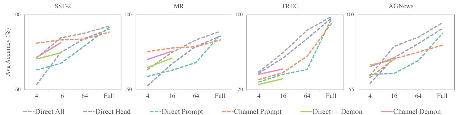
Figure 3: Varying the number of training examples ($K$). All models use GPT-2 Large. All, Head and Prompt indicate finetuning all parameters of the LM, head tuning and prompt tuning, respectively. Direct++ Demon and Channel Demon indicate demonstration-based methods (the best out of concat-based and ensemble-based is taken). Models are run 4 times for $K=\mathrm{full}$ (4 verbalizers) and 20 times for others (4 verbalizers and 5 data seeds). Channel models are more competitive with smaller $K$; less competitive with larger $K$.

6.3 Ablations

For the ablations, we report experiments on SST-2, MR, TREC and AGNews, using one train seed (instead of four), and four verbalizers and five data seeds (as in main experiments).

Varying the number of training examples

We vary the number of training examples ($K$) and report the average accuracy in Figure 3. All methods achieve higher accuracy as $K$ increases. While we confirm strong performance of channel prompt tuning with $K\leq 16$, head tuning outperforms channel head tuning when $K=64$. When $K=\mathrm{Full}$, both direct prompt tuning and head tuning outperform channel prompt tuning. We think this is because (1) training signals amplified by channel models (Lewis and Fan, 2018) are more significant when $K$ is small, and (2) channel models are more beneficial when labels on the training data are imbalanced (confirmed in the next ablation), which is more likely to happen with smaller $K$.

It is also worth noting that our experiment with $K=\mathrm{Full}$ confirms the finding from Lester et al. (2021) that direct prompt tuning matches the performance of all finetuning—finetuning all parameters of the LM—while being much more parameter-efficient. This only holds with $K=\mathrm{Full}$; in a few-shot setup, all finetuning significantly outperforms other methods. This contradicts traditional analysis that having less trainable parameters is better when the training data is scarce (Ng and Jordan, 2002). It is likely because such analysis did not take into account language model pretraining, which gives supervision to the model yet is not the training data for an end task.

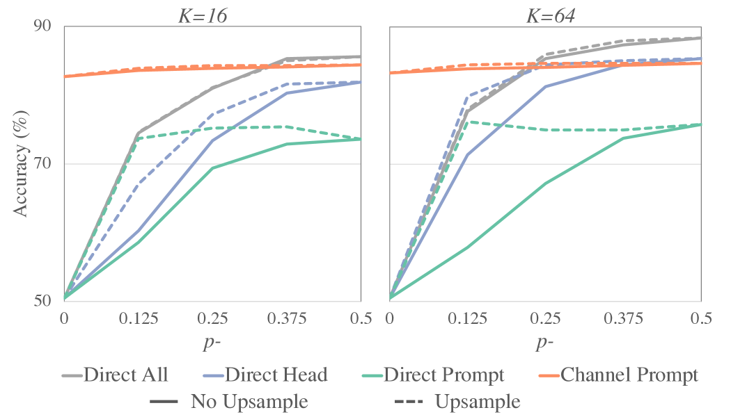
Figure 4: Impact of imbalance in labels. The average accuracy on SST-2 and MR of different methods with varying ratios of negative labels on the training data (denoted as $p^{-}$), when $K=16$ (left) or $64$ (right). As $p^{-}$ increases, the data is more balanced. Channel models are more robust to imbalanced training data.

Impact of imbalance in labels

On binary datasets (SST-2 and MR), we vary the label imbalance in the training data with $K=\{16,64\}$. Specifically, let $\mathcal{C}=\{c^{+},c^{-}\}$ and $p^{-}=|\{(x,c)\in\mathcal{D}|c=c^{-}\}|/|\mathcal{D}|$, i.e., the ratio of $c^{-}$ in the training data. We vary $p^{-}$ to be $\{0,0.125,0.250,0.375,0.5\}$. $p^{-}=0.5$ means the labels are perfectly balanced, and $p^{-}=0$ means that labels in the training data only include $c^{+}$. We additionally compare with upsampling baselines where we upsample training examples with infrequent labels so that the model has seen an equal number of examples per label during training.

Data	Zero-shot		Finetuning
	Direct++	Channel	Direct All	Direct Head	Direct Trans	Direct Prompt	Channel Prompt
SST-2	80.3/76.9	77.1/74.8	50.2/49.1	50.2/49.1	50.2/49.1	50.2/49.1	85.5/82.5
SST-5	33.3/28.8	29.2/27.7	40.1/34.8	34.3/28.0	32.6/24.5	30.0/18.1	37.5/32.6
MR	77.4/73.2	74.3/69.3	50.0/50.0	50.0/50.0	50.0/50.0	50.0/50.0	80.9/74.8
CR	77.9/69.7	65.8/60.2	50.0/50.0	50.0/50.0	50.0/50.0	50.0/50.0	80.9/74.8
TREC	27.7/12.6	30.5/19.4	50.8/31.0	44.8/29.6	44.6/32.8	33.9/17.4	34.3/26.0
Subj	52.0/48.8	57.8/51.5	50.0/50.0	50.0/50.0	50.0/50.0	50.0/50.0	66.6/57.6

Table 5: Model performance when there is at least one label at test time that was unseen during training. All models are run 20 times (4 verbalizers and 5 data seeds). All, Head, Trans and Prompt indicate finetuning all parameters of the LM, head tuning, transformation tuning and prompt tuning, respectively. We report the average and the worst-case accuracy, separated by a slash.

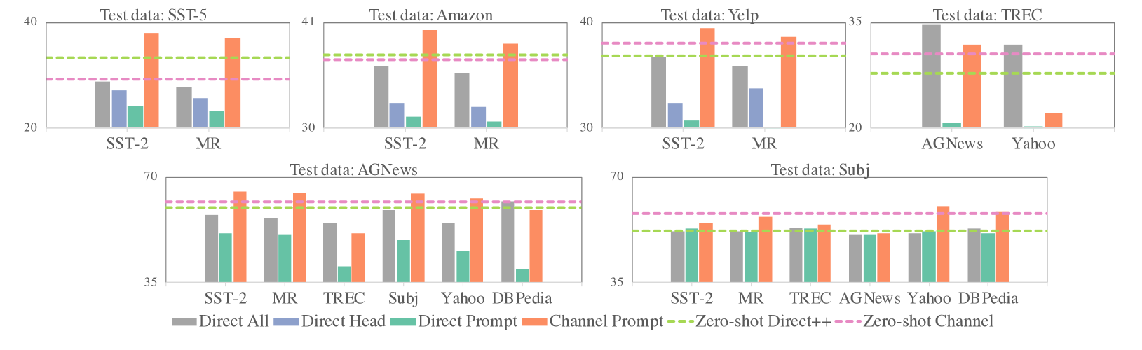
Figure 5: Model performance when transferred to unseen data, where x-axis indicates training data. Direct Head is not applicable when label space is not shared (when test datasets are TREC, AGNews and Subj). Channel models have better generalization capacity than direct models.

Results are reported in Figure 4. All direct models are sensitive to the imbalance in training data, even though they benefit from upsampling when $p^{-}$ is small. Channel prompt tuning is insensitive to the imbalance, and significantly outperforms direct models when $p^{-}$ is small; it even outperforms all finetuning when $p^{-}<0.25$. When $p^{-}$ is near to 0.5, direct head tuning matches or outperforms channel prompt tuning.

It is also worth noting that direct prompt tuning with upsampling matches or outperforms all finetuning and head tuning when $p^{-}$ is small.

6.4 Generalization to unseen labels

We experiment with a challenging scenario where the model must generalize to unseen labels. While it may be seen as an extreme scenario, this is often a practical setting, e.g., the problem is defined with a set of labels but later an addition of the new label may be needed.

First, we sample $K$ training examples as in main experiments but excluding one random label, so that at least one label at test time was unseen during training. Table 5 reports the results. All direct models are unable to predict the label that is unseen at training time. However, channel prompt tuning can predict unseen labels and achieves considerably better performance than zero-shot. It outperforms all finetuning on 2-way classification datasets, and outperforms head tuning on five datasets except for TREC on which head tuning achieves very strong performance on seen labels.

Next, we run zero-shot transfer learning, where the model is trained on one dataset and is tested on another dataset. Here, head tuning is not applicable when the labels are not shared between two datasets. Figure 5 shows the results. Channel prompt tuning outperforms all direct models including all finetuning on all datasets except for TREC. It is particularly competitive when the tasks are inherently similar, e.g., transfer between 2-way sentiment analysis and 5-way sentiment analysis in the first three figures. In fact, in such cases, performance is close to the models trained on in-domain data. When tasks are inherently different, e.g., the rest of the figures in Figure 5, gains over zero-shot performance are relatively small; we think more work should be done to make cross-task transfer better and to discover when it is possible.

7 Discussion & Conclusion

In this work, we introduced a noisy channel approach for few-shot text classification through LM prompting, where we either provide demonstrations to the LM or tune the prompt embeddings in the continuous space. Our experiments on eleven datasets show that channel models significantly outperform their direct counterparts, mainly because of their stability, i.e., lower variance and better worst-case accuracy. We also found that direct head tuning is more competitive than previously thought, and different methods are preferred given different conditions. Specifically, channel prompt tuning is preferred in the following scenarios.

$K$ is small

Channel prompt tuning is more competitive when there are fewer training examples. We hypothesize two reasons: (1) Channel models are more stable (i.e., achieve low variance and high worst-case accuracy), unlike direct models that are highly unstable with small $k$ (Zhao et al., 2021; Perez et al., 2021; Lu et al., 2021). (2) Channel models provide more signals by requiring the model to explain the input word-by-word (as claimed in Lewis and Fan (2018)) which is beneficial in the low data regime.

Data is imbalanced or $|\mathcal{C}|$ is large

When the training data is even slightly imbalanced, no direct models are competitive. We think this is because the LM head relies too much on unconditional distributions of labels. Channel prompt tuning is less sensitive because labels are only a conditioning variable. Label imbalance in the training data is a real-world problem, especially when $k$ is small and $|\mathcal{C}|$ is large. We thus suggest this is an important area for future work.

Generalization to unseen labels is required

All direct models are unable to predict labels that are unseen during training, indicating that they overfit in the label space. In contrast, channel models can predict unseen labels, likely because the label space is indirectly modeled. This is in line with prior work that shows channel models are more competitive under a distribution shift (Yogatama et al., 2017; Lewis and Fan, 2018).

Task is closer to language modeling

If the task is too different from language modeling even with carefully chosen verbalizers (e.g., TREC and Subj), head tuning outperforms prompt tuning. This is likely because it benefits from directly updating the parameters of the LM. This may mean that causal LMs are not suitable for all tasks, or we need more sophisticated methods to apply causal LMs for such tasks without updating the LM parameters.

Limitations and future work

While we show that channel models are competitive in few-shot text classification, there are limitations that provide avenues for future work. First, it is not as easy to use channel models for non classification tasks where modeling prior distributions is non-trivial. We think future work can obtain the prior with a separate model and incorporate it to the conditional LM as done by Lewis and Fan (2018), potentially with beam search decoding as in Yu et al. (2017); Yee et al. (2019).

Second, while this paper focuses on causal LMs, it is an open question how to use a channel model with masked LMs. Although we think channel models are not inherently restricted to causal LMs, the specific way in which existing masked LMs are pretrained makes it hard to use channel models without updating the LM parameters, e.g., masked LMs are not trained to generate long sentences. One recent approach uses a label-conditioning objective (Tam et al., 2021) as a clever way to introduce a channel-like model with existing masked LMs. Extending and further integrating these different approaches would be important for using channel models in a wider range of scenarios.

Appendix A Samples & Verbalizers

Table 10 shows samples from each dataset. Table 6 shows a list of verbalizers (four for each dataset), mainly taken from Gao et al. (2021) and label words included in the original data.

Dataset	Verbalizers
SST-2, MR	A MASK one.; It was MASK.; All in all MASK.; A MASK piece. (MASK={great, terrible})
SST-5, Amaon, Yelp	(Same as above.) (MASK={great,good,okay,bad terrible})
TREC	MASK: ; Q: MASK: ; Why MASK? ; Answer: MASK (MASK={Description, Entity, Expression, Human, Location, Number})
AGNews	Topic: MASK.; Subject: MASK.; This is about MASK.; It is about MASK. (MASK={World, Sports, Business, Technology})
Yahoo	(Same as above) (MASK={Society & Culture, Science & Mathematics, Health, Education & Reference, Computers & Internet, Sports, Business & Finance, Entertainment & Music, Family & Relationships, Politics & Government})
DBPedia	(Same as above) (MASK={Company, Educational Institution, Artist, Athlete, Office Holder, Mean of Transportation, Building, Natural Place, Village, Animal, Plant, Album, Film, Written Work})
Subj	This is MASK.; It’s all MASK.’ It’s MASK.; Is it MASK? (MASK={subjective, objective})

Table 6: Four different verbalizers for each dataset used in the experiments, separated by ‘;’. Verbalizers are taken from Gao et al. (2021) and label words included in the original data.

Data	Direct			Channel
	Head	Trans	Prompt	Prompt
SST-2, SST-5	0.001	0.001	0.01	0.001
MR	0.001	0.001	0.01	0.1
CR	0.001	0.001	0.01	0.001
Amazon	0.001	0.001	0.001	0.1
Yelp	0.001	0.001	0.001	0.01
TREC	0.001	0.001	0.01	0.01
AGNews	0.001	0.001	0.01	0.1
Yahoo	0.001	0.001	0.01	0.001
DBPedia	0.001	0.001	0.01	0.01
Subj	0.001	0.001	0.01	0.01

Table 7: Learning rates of the models in Table 4.

Data	Size	Direct		Channel
		Head	Prompt	Prompt
SST-2	S,M,XL	0.001	0.01	0.001
MR	S,M,XL	0.001	0.01	0.1
TREC	S	0.01	0.01	0.1
TREC	M	0.01	0.01	1.0
TREC	XL	0.001	0.01	0.1
AGNews	S	0.001	0.01	0.1
AGNews	M	0.001	0.01	0.01
AGNews	XL	0.001	0.01	0.001

Table 8: Learning rates of the models in Figure 6.

Data	$k$	Direct		Channel
		Head	Prompt	Prompt
SST-2	4	0.001	0.001	0.001
SST-2	64	0.001	0.01	0.001
SST-2	$\mathrm{Full}$	0.001	0.01	0.1
MR	4	0.001	0.001	0.001
MR	64,$\mathrm{Full}$	0.001	0.01	0.1
TREC	4	0.001	0.001	0.001
TREC	64,$\mathrm{Full}$	0.001	0.01	0.1
AGNews	4	0.001	0.001	0.1
AGNews	64	0.001	0.01	0.01
AGNews	$\mathrm{Full}$	0.001	0.01	0.1

Table 9: Learning rates of the models in Figure 3.

Data: SST-2, SST-5 and MR (Movie Sentiment Analysis)

•  A three-hour cinema master class. ($c=$terrible)

•  A pretensions – and disposable story — sink the movie. ($c=$great)

Data: CR

•  It is slow, if you keep the original configuration and prigs (why’d u buy it then?!) it’ll run smoothly, but still slower

then most other coloured-screen nokias. ($c=$terrible)

•  It takes excellent pics and is very easy to use, if you read the manual. ($c=$great)

Data: Amazon

•  Don’t waste your money if you already have 2003… There isn’t one reason to get this update if you already have MS

Money 2003 Deluxe and Business. ($c=$terrible)

•  The game was in perfect condition! came before it said it should have by 2 days!! I love the game and I suggest it to

a lot of my friends!! ($c=$great)

Data: Yelp

•  I’ve eaten at the other location, and liked it. But I tried this place, and I have JUST NOW recovered physically enough

from the worst food poisoning I’ve ever heard of to write this review. ($c=$terrible)

•  Great ambiance, awesome appetizers, fantastic pizza, flawless customer service. ($c=$great)

Data: TREC

•  How do you get a broken cork out of a bottle? ($c=$Description)

•  Mississippi is nicknamed what? ($c=$Entity)

•  What is BPH? ($c=$Expression)

•  Who won the Novel Peace Prize in 1991? ($c=$Human)

•  What stadium do the Miami Dolphins play their home games in? ($c=$Location)

•  How long did the Charles Manson murder trial last? ($c=$Number)

Data: AGNews

•  Peru Rebel Leader Offers to Surrender Reuters - The leader of an armed group which took over a police station in a

southern Peruvian town three days ago and demanded the president’s resignation … ($c=$World)

•  Walk in park for Yankees Drained by a difficult week, the New York Yankees needed an uplifting victory. ($c=$Sports)

•  Schwab plans new, smaller branches SAN FRANCISCO – Charles Schwab & Co. is opening new offices that are

smaller than its current branches … ($c=$Business)

•  NASA Mountain View claims world’s fastest computer. ($c=$Technology)

Data: Yahoo

•  What’s one change you could make to your lifestyle that would give you more peace? … ($c=$Society & Culture)

•  If the average for a test was 74% and the standard deviation was 13, are you within 1 SD if you scored a 62?

($c=$Science & Mathematics)

•  Can someone explain to me what IndexOf is in Visual Basic? ($c=$Computers & Internet)

Data: DBPedia

•  Coca-Cola Bottling Co. Consolidated headquartered in Charlotte North Carolina is the largest independent Coca-

Cola bottler in the United States … ($c=$Company)

•  Elk County Catholic High School is a private Roman Catholic high school in … ($c=$Educational Institution)

•  Louis Wiltshire (born 23 April 1969) is a British sculptor. … ($c=$Artist)

•  Russel Paul Kemmerer (botn November 1 1931 in Pittsburgh Pennsylvania) is an American retired professional

baseball player. ($c=$Athlete)

•  Dialectica aemula is a moth of the Gracillariidae family. … ($c=$Animal)

•  Ephedra viridis known by the common names green Mormon tea green ephedra is a species of Ephedra. ($c=$Plant)

Data: Subj

•  As i settled into my world war ii memory, i found myself strangely moved by even the corniest and most hackneyed

contrivances. ($c=$subjective)

•  This is a story about the warm relationship between a little girl and her father despite the difficult conditions they

have to live in. ($c=$objective)

Table 10: Samples from each dataset. $c$ indicates the label.

Appendix B Implementation Details

We use PyTorch (Paszke et al., 2019) and Huggingface Transformers (Wolf et al., 2020). For MR, we use the sentence polarity dataset version 1.0. We use the batch size of 32 and the sequence length of 128 for datasets with short input text (SST-2, SST-5, MR, TREC) and the batch size of 16 and the sequence length of 256 for datasets with long input text (AGNews, Amazon, Yelp, DBPedia, Yahoo, Subj). When the concat-based demonstration method is used, the sequence length is multiplied by the number of training examples, yet is bounded by 1024 which is a strict limit of GPT-2.

For all finetuning experiments, we train the model for 100 global steps. We use the loss divided by the number of all tokens in the batch. We use Adam optimizer (Kingma and Ba, 2015) with no weight decay and no warmup steps. For head tuning, transformation tuning and prompt tuning, we use the learning rate $\{0.1,0.01,0.001\}$ and choose the one that gives the lowest training loss on average in order to eliminate the need of the validation data. The chosen learning rate values are reported in Table 7. For all finetuning, we use the learning rate of $10^{-5}$. For prompt tuning, we use $n=20$ prompt tokens which embeddings are initialized from a random subset of the top $5000$ vocabularies, following the original paper (Lester et al., 2021).

Data	Direct			Direct++			Channel
	Avg${}_{\text{(Std)}}$	Best	Worst	Avg${}_{\text{(Std)}}$	Best	Worst	Avg${}_{\text{(Std)}}$	Best	Worst
SST-2	58.9(9.4)	77.4	50.6	66.8(8.2)	81.0	51.7	85.0(1.1)	86.9	83.1
SST-5	27.6(5.2)	40.9	23.0	23.7(4.5)	31.4	14.4	36.2(2.1)	39.6	32.7
MR	56.4(8.5)	78.2	50.0	60.2(8.6)	79.0	50.5	80.5(1.8)	83.2	76.8
CR	54.7(7.9)	78.8	50.0	66.8(9.8)	84.0	50.0	80.8(3.3)	86.2	74.8
Amazon	33.0(6.5)	43.6	21.4	40.8(2.5)	46.4	35.7	39.4(2.5)	42.6	34.3
Yelp	32.6(5.1)	41.6	23.3	38.5(3.6)	44.0	31.6	39.8(2.1)	43.8	36.5
AGNews	34.0(10.9)	62.3	25.0	51.2(10.2)	68.0	34.4	68.5(4.5)	76.1	60.6
TREC	27.2(9.2)	42.0	9.4	31.6(18.9)	78.4	13.0	42.0(7.1)	54.4	26.8
Yahoo	13.0(2.6)	18.7	10.0	29.6(6.2)	40.7	19.4	56.2(1.2)	57.7	52.3
DBPedia	32.5(17.0)	68.2	7.1	71.1(8.0)	82.4	55.2	58.5(12.5)	74.3	40.0
Subj	53.7(6.0)	71.8	49.9	56.9(8.2)	75.9	50.0	60.5(6.5)	68.0	40.8
Avg.	38.5	56.7	29.1	48.8	64.7	36.9	58.9	64.8	50.8

Table 11: Full results from demonstration methods when a concat-based method is used; analogous to Table 3. Avg, Std, Best and Worst indicate the average accuracy, standard deviation, the best-case accuracy and the worst-case accuracy, respectively. Bold: Best when combined with Table 12.

Data	Direct			Direct++			Channel
	Avg${}_{\text{(Std)}}$	Best	Worst	Avg${}_{\text{(Std)}}$	Best	Worst	Avg${}_{\text{(Std)}}$	Best	Worst
SST-2	57.5(9.6)	84.2	50.9	79.7(5.8)	88.3	68.0	77.5(7.9)	85.9	59.5
SST-5	25.6(2.7)	34.6	23.2	33.8(5.8)	42.4	23.3	33.6(2.2)	38.0	30.2
MR	58.8(9.9)	82.9	50.0	76.8(6.4)	85.7	60.1	76.1(6.6)	82.0	60.0
CR	51.0(2.2)	59.0	50.0	72.8(12.0)	87.4	54.6	79.7(4.2)	84.0	69.3
Amazon	31.7(6.1)	44.5	23.1	39.8(4.6)	47.8	32.0	40.4(2.1)	44.3	36.2
Yelp	31.4(6.3)	41.4	23.6	39.2(6.1)	47.3	29.6	41.5(1.3)	43.5	38.5
AGNews	51.9(9.8)	69.7	34.2	73.1(6.2)	81.8	58.6	74.3(2.7)	78.5	69.3
TREC	32.1(10.4)	54.4	13.0	22.9(10.1)	44.4	9.8	31.5(5.0)	43.2	23.8
Yahoo	16.6(4.2)	24.6	10.7	50.6(2.1)	54.1	46.5	58.6(0.7)	59.7	57.4
DBPedia	46.8(15.2)	63.0	17.1	72.6(7.0)	81.9	55.7	64.8(3.5)	70.0	57.0
Subj	51.6(3.4)	62.3	49.6	52.2(5.4)	61.8	41.8	52.4(3.0)	57.7	46.9
Avg.	41.4	56.4	31.4	55.8	65.7	43.6	57.3	62.4	49.8

Table 12: Full results from demonstration methods when a ensemble-based method is used; analogous to Table 3. Avg, Std, Best and Worst indicate the average accuracy, standard deviation, the best-case accuracy and the worst-case accuracy, respectively. Bold: Best when combined with Table 11.

Data	Direct Head			Direct Trans			Direct Prompt			Channel Prompt
	Avg${}_{\text{(Std)}}$	Best	Worst	Avg${}_{\text{(Std)}}$	Best	Worst	Avg${}_{\text{(Std)}}$	Best	Worst	Avg${}_{\text{(Std)}}$	Best	Worst
SST-2	80.2(5.1)	88.4	68.6	77.3(5.6)	87.7	57.5	72.6(10.0)	89.3	50.9	85.8(1.5)	88.3	81.3
SST-5	34.9(2.8)	40.1	30.0	33.0(2.7)	40.0	25.5	30.9(5.8)	42.6	19.1	36.3(3.0)	41.6	27.9
MR	73.7(7.7)	83.9	56.4	71.3(8.1)	83.2	51.6	67.4(9.9)	85.1	50.1	81.7(1.4)	84.2	78.0
CR	67.6(10.5)	84.0	50.0	63.9(9.6)	84.5	50.0	65.7(13.2)	87.4	50.0	79.6(1.4)	82.7	76.4
Amazon	34.5(3.5)	41.4	28.8	32.1(4.6)	40.2	18.2	31.2(5.7)	43.6	20.0	43.4(2.3)	49.2	39.2
Yelp	40.6(4.0)	46.9	32.8	38.9(3.3)	46.3	31.5	31.9(7.7)	45.0	20.6	43.9(2.2)	47.2	37.2
TREC	54.1(7.1)	71.2	42.4	48.0(7.4)	66.6	31.0	35.9(11.8)	65.8	13.0	37.1(7.3)	55.8	20.8
AGNews	74.1(6.6)	84.5	61.2	66.9(8.0)	83.5	47.0	61.9(15.9)	83.5	25.2	73.4(3.1)	77.9	63.9
Yahoo	39.1(3.2)	44.9	31.4	33.8(4.5)	43.8	23.0	27.4(5.6)	39.0	15.7	54.0(2.0)	57.6	46.7
DBPedia	49.3(7.7)	64.2	37.5	42.4(6.8)	56.9	28.6	41.8(13.3)	75.3	9.9	67.7(5.7)	78.3	52.9
Subj	86.3(3.0)	90.9	79.1	86.0(4.0)	90.8	71.6	65.5(7.7)	78.7	49.9	75.5(5.0)	84.5	58.8
Avg.	57.7	67.3	47.1	54.0	65.8	39.6	48.4	66.9	29.5	61.7	67.9	53.0

Table 13: Full results from tuning methods; analogous to Table 4. Head, Trans, Prompt indicate head tuning, transformation tuning and prompt tuning, respectively. Avg, Std, Best and Worst indicate the average accuracy, standard deviation, the best-case accuracy and the worst-case accuracy, respectively.

Appendix C Additional Results

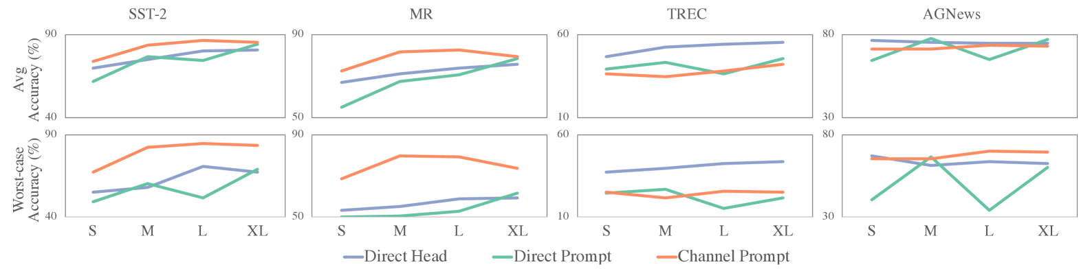
Figure 6: Varying the size of LMs from GPT-2 Small to GPT-2 X-Large. The average accuracy (top) and the worst-case accuracy (bottom) are reported. All models are run 20 times (4 verbalizers and 5 data seeds). Head and Prompt indicate head tuning and prompt tuning, respectively. Trends are consistent across different sizes of LM.

More metrics

Table 11, 12 and 13 report the average accuracy, the variance, the best-case accuracy and the worst-case accuracy using the concat-based demonstration, the ensemble-based demonstration and the tuning methods, respectively. Results consistently indicate that channel models achieve significantly lower variance and higher worst-case accuracy. The best-case accuracy is often achieved by direct models, but channel models outperform direct models on average.

Varying the size of LMs

We vary the size of LMs and report the average and the worst-case accuracy in Figure 6. The trends—no matter the best performance is achieved by channel prompt tuning or direct head tuning—are fairly consistent across varying size of LMs.

References

- Asri et al. (2016) Hiba Asri, H. Mousannif, H. A. Moatassime, and Thomas Noël. 2016. Using machine learning algorithms for breast cancer risk prediction and diagnosis. In ANT/SEIT.
- Bansal et al. (2020) Trapit Bansal, Rishikesh Jha, Tsendsuren Munkhdalai, and Andrew McCallum. 2020. Self-supervised meta-learning for few-shot natural language classification tasks. In EMNLP.
- Brown et al. (1993) Peter F Brown, Stephen A Della Pietra, Vincent J Della Pietra, and Robert L Mercer. 1993. The mathematics of statistical machine translation: Parameter estimation. Computational linguistics.
- Brown et al. (2020) Tom Brown, Benjamin Mann, Nick Ryder, Melanie Subbiah, Jared D Kaplan, Prafulla Dhariwal, Arvind Neelakantan, Pranav Shyam, Girish Sastry, Amanda Askell, Sandhini Agarwal, Ariel Herbert-Voss, Gretchen Krueger, Tom Henighan, Rewon Child, Aditya Ramesh, Daniel Ziegler, Jeffrey Wu, Clemens Winter, Chris Hesse, Mark Chen, Eric Sigler, Mateusz Litwin, Scott Gray, Benjamin Chess, Jack Clark, Christopher Berner, Sam McCandlish, Alec Radford, Ilya Sutskever, and Dario Amodei. 2020. Language models are few-shot learners. In NeurIPS.
- Chen et al. (2020) Jiaao Chen, Zichao Yang, and Diyi Yang. 2020. MixText: Linguistically-informed interpolation of hidden space for semi-supervised text classification. In ACL.
- Clark et al. (2018) Kevin Clark, Minh-Thang Luong, Christopher D Manning, and Quoc V Le. 2018. Semi-supervised sequence modeling with cross-view training. In EMNLP.
- Ding and Gimpel (2019) Xiaoan Ding and Kevin Gimpel. 2019. Latent-variable generative models for data-efficient text classification. In EMNLP.
- Finn et al. (2017) Chelsea Finn, Pieter Abbeel, and Sergey Levine. 2017. Model-agnostic meta-learning for fast adaptation of deep networks. In ICML.
- Gao et al. (2021) Tianyu Gao, Adam Fisch, and Danqi Chen. 2021. Making pre-trained language models better few-shot learners. In ACL.
- Guo et al. (2017) Chuan Guo, Geoff Pleiss, Yu Sun, and Kilian Q Weinberger. 2017. On calibration of modern neural networks. In ICML.
- Holtzman et al. (2021) Ari Holtzman, Peter West, Vered Schwartz, Yejin Choi, and Luke Zettlemoyer. 2021. Surface form competition: Why the highest probability answer isn’t always right. In EMNLP.
- Houlsby et al. (2019) Neil Houlsby, Andrei Giurgiu, Stanislaw Jastrzebski, Bruna Morrone, Quentin De Laroussilhe, Andrea Gesmundo, Mona Attariyan, and Sylvain Gelly. 2019. Parameter-efficient transfer learning for nlp. In ICML.
- Hu and Liu (2004) Minqing Hu and Bing Liu. 2004. Mining and summarizing customer reviews. In Proceedings of the Tenth ACM SIGKDD International Conference on Knowledge Discovery and Data Mining.
- Huang et al. (2018) Po-Sen Huang, Chenglong Wang, Rishabh Singh, Wen-tau Yih, and Xiaodong He. 2018. Natural language to structured query generation via meta-learning. In NAACL.
- Jiang et al. (2020) Zhengbao Jiang, Frank F Xu, Jun Araki, and Graham Neubig. 2020. How can we know what language models know? TACL.
- Kingma and Ba (2015) Diederik P Kingma and Jimmy Ba. 2015. Adam: A method for stochastic optimization. In ICLR.
- Koehn et al. (2003) Philipp Koehn, Franz J Och, and Daniel Marcu. 2003. Statistical phrase-based translation. In NAACL-HLT.
- Le Scao and Rush (2021) Teven Le Scao and Alexander Rush. 2021. How many data points is a prompt worth? In NAACL-HLT.
- Lehmann et al. (2015) Jens Lehmann, Robert Isele, Max Jakob, Anja Jentzsch, Dimitris Kontokostas, Pablo N Mendes, Sebastian Hellmann, Mohamed Morsey, Patrick Van Kleef, Sören Auer, et al. 2015. Dbpedia–a large-scale, multilingual knowledge base extracted from wikipedia. Semantic web.
- Lester et al. (2021) Brian Lester, Rami Al-Rfou, and Noah Constant. 2021. The power of scale for parameter-efficient prompt tuning. In EMNLP.
- Lewis and Fan (2018) Mike Lewis and Angela Fan. 2018. Generative question answering: Learning to answer the whole question. In ICLR.
- Li and Liang (2021) Xiang Lisa Li and Percy Liang. 2021. Prefix-tuning: Optimizing continuous prompts for generation. In ACL.
- Liu et al. (2021) Xiao Liu, Yanan Zheng, Zhengxiao Du, Ming Ding, Yujie Qian, Zhilin Yang, and Jie Tang. 2021. Gpt understands, too. arXiv preprint arXiv:2103.10385.
- Logan IV et al. (2021) Robert L Logan IV, Ivana Balaževic, Eric Wallace, Fabio Petroni, Sameer Singh, and Sebastian Riedel. 2021. Cutting down on prompts and parameters: Simple few-shot learning with language models. arXiv preprint arXiv:2106.13353.
- Lu et al. (2021) Yao Lu, Max Bartolo, Alastair Moore, Sebastian Riedel, and Pontus Stenetorp. 2021. Fantastically ordered prompts and where to find them: Overcoming few-shot prompt order sensitivity. arXiv preprint arXiv:2104.08786.
- McAuley and Leskovec (2013) Julian McAuley and Jure Leskovec. 2013. Hidden factors and hidden topics: understanding rating dimensions with review text. In Proceedings of the 7th ACM conference on Recommender systems, pages 165–172.
- Miyato et al. (2017) Takeru Miyato, Andrew M Dai, and Ian Goodfellow. 2017. Adversarial training methods for semi-supervised text classification. In ICLR.
- Ng and Jordan (2002) Andrew Y Ng and Michael I Jordan. 2002. On discriminative vs. generative classifiers: A comparison of logistic regression and naive bayes. In NeurIPS.
- Pang and Lee (2004) Bo Pang and Lillian Lee. 2004. A sentimental education: Sentiment analysis using subjectivity summarization based on minimum cuts. In ACL.
- Pang and Lee (2005) Bo Pang and Lillian Lee. 2005. Seeing stars: Exploiting class relationships for sentiment categorization with respect to rating scales. In ACL.
- Paszke et al. (2019) Adam Paszke, Sam Gross, Francisco Massa, Adam Lerer, James Bradbury, Gregory Chanan, Trevor Killeen, Zeming Lin, Natalia Gimelshein, Luca Antiga, et al. 2019. Pytorch: An imperative style, high-performance deep learning library. In NeurIPS.
- Perez et al. (2021) Ethan Perez, Douwe Kiela, and Kyunghyun Cho. 2021. True few-shot learning with language models. In NeurIPS.
- Qin and Eisner (2021) Guanghui Qin and Jason Eisner. 2021. Learning how to ask: Querying lms with mixtures of soft prompts. In NAACL-HLT.
- Radford et al. (2019) Alec Radford, Jeffrey Wu, Rewon Child, David Luan, Dario Amodei, and Ilya Sutskever. 2019. Language models are unsupervised multitask learners. OpenAI blog.
- Rebuffi et al. (2017) Sylvestre-Alvise Rebuffi, Hakan Bilen, and Andrea Vedaldi. 2017. Learning multiple visual domains with residual adapters. In NeurIPS.
- Shannon (1948) Claude Elwood Shannon. 1948. A mathematical theory of communication. The Bell system technical journal.
- Shin et al. (2020) Taylor Shin, Yasaman Razeghi, Robert L Logan IV, Eric Wallace, and Sameer Singh. 2020. Autoprompt: Eliciting knowledge from language models with automatically generated prompts. In EMNLP.
- Socher et al. (2013) Richard Socher, Alex Perelygin, Jean Wu, Jason Chuang, Christopher D Manning, Andrew Y Ng, and Christopher Potts. 2013. Recursive deep models for semantic compositionality over a sentiment treebank. In EMNLP.
- Tam et al. (2021) Derek Tam, Rakesh R Menon, Mohit Bansal, Shashank Srivastava, and Colin Raffel. 2021. Improving and simplifying pattern exploiting training. In EMNLP.
- Voorhees and Tice (2000) Ellen M Voorhees and Dawn M Tice. 2000. Building a question answering test collection. In SIGIR.
- Wolf et al. (2020) Thomas Wolf, Lysandre Debut, Victor Sanh, Julien Chaumond, Clement Delangue, Anthony Moi, Pierric Cistac, Tim Rault, Rémi Louf, Morgan Funtowicz, Joe Davison, Sam Shleifer, Patrick von Platen, Clara Ma, Yacine Jernite, Julien Plu, Canwen Xu, Teven Le Scao, Sylvain Gugger, Mariama Drame, Quentin Lhoest, and Alexander M. Rush. 2020. Transformers: State-of-the-art natural language processing. In EMNLP: System Demonstrations.
- Xie et al. (2020) Qizhe Xie, Zihang Dai, Eduard Hovy, Minh-Thang Luong, and Quoc V Le. 2020. Unsupervised data augmentation for consistency training. In NeurIPS.
- Yamada and Knight (2001) Kenji Yamada and Kevin Knight. 2001. A syntax-based statistical translation model. In ACL.
- Yee et al. (2019) Kyra Yee, Nathan Ng, Yann N Dauphin, and Michael Auli. 2019. Simple and effective noisy channel modeling for neural machine translation. In EMNLP.
- Yogatama et al. (2017) Dani Yogatama, Chris Dyer, Wang Ling, and Phil Blunsom. 2017. Generative and discriminative text classification with recurrent neural networks. arXiv preprint arXiv:1703.01898.
- Yu et al. (2017) Lei Yu, Phil Blunsom, Chris Dyer, Edward Grefenstette, and Tomas Kocisky. 2017. The neural noisy channel. In ICLR.
- Zhang et al. (2015) Xiang Zhang, Junbo Zhao, and Yann LeCun. 2015. Character-level convolutional networks for text classification. In NeurIPS.
- Zhao et al. (2021) Tony Z Zhao, Eric Wallace, Shi Feng, Dan Klein, and Sameer Singh. 2021. Calibrate before use: Improving few-shot performance of language models. In ICML.
- Zhong et al. (2021) Zexuan Zhong, Dan Friedman, and Danqi Chen. 2021. Factual probing is [mask]: Learning vs. learning to recall. In NAACL-HLT.