Classification and Visualization of
Genotype $\times$ Phenotype Interactions in Biomass Sorghum

Abstract

We introduce a simple approach to understanding the relationship between single nucleotide polymorphisms (SNPs), or groups of related SNPs, and the phenotypes they control. The pipeline involves training deep convolutional neural networks (CNNs) to differentiate between images of plants with reference and alternate versions of various SNPs, and then using visualization approaches to highlight what the classification networks key on. We demonstrate the capacity of deep CNNs at performing this classification task, and show the utility of these visualizations on RGB imagery of biomass sorghum captured by the TERRA-REF gantry. We focus on several different genetic markers with known phenotypic expression, and discuss the possibilities of using this approach to uncover unknown genotype $\times$ phenotype relationships.

1 Introduction

Sorghum is a cereal crop, used worldwide for a variety of purposes including for use as grain and as a source of biomass for bio-energy production, which is the context we primarily focus on in this paper. For biofuel production, the goal of both plant growers and breeders is to produce sorghum crops that grow as big as possible, as quickly as possible, with as few resources as possible. Plant breeders produce new lines of sorghum by crossing together candidate lines that have desirable traits, or known genes that correspond to desirable traits.

In this paper, we propose a simple pipeline for understanding and identifying interesting genetic markers that control visually observable traits. This pipeline could be leveraged by plant geneticists and breeders to understand the relationship between single nucleotide polymorpishms (SNPs, locations in the organism’s DNA that vary between different members of the population), or groups of related SNPs, and the phenotypes that they impact.

The pipeline involves:

• Identifying candidate SNPs, or groups of SNPs, of interest in the sorghum genome;

• Training deep convolutional neural networks (CNNs) on visual sensor data to differentiate between reference and alternate versions of the SNP; and

• Visualizing what visual features led to a reference or alternate classification by the CNN.

We demonstrate the feasibility and utility of this pipeline on a number of SNPs identified in the sorghum Bioenergy Association Panel [8] (BAP), a set of 390 sorghum cultivars whose genomes have been fully sequenced and which show promise for bio-energy usage.

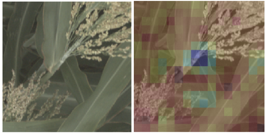
Figure 1: We train deep convolutional neural network classifiers to predict whether an image of a sorghum crop contains a reference or alternate version of particular genetic marker, and then visualize why the network makes that prediction. In this figure, we show the visualization for why the neural network predicted an image showed a plant with a reference version of a SNP that controls leaf wax composition – the visualization highlights the especially waxy part of the stem.

2 Background

2.1 Sorghum and Polymorphisms

Sorghum is a diploid species, meaning that it has two copies of each of its 10 chromosomes. Each chromosome consists of DNA, the genetic instructions for the plant. The DNA itself is made up of individual nucleotides, sequences of which tell the plant precisely which proteins to make. Variations in these sequences, called single nucleotide polymorphisms, can result in changes to the proteins the plant is instructed to make, which in turn can have varying degrees of impact on the structure and performance of the plant. Understanding the impact that specific genes have on plants and how they interact with their environment is a fundamental problem and area of study in plant biology [6, 7, 13, 35].

Single nucleotide polymorphisms (SNPs) are specific variations that exist between different members of a population at a single location on the chromosome, where one adenine, thymine, cytosine or guanine nucleotide in one plant may be have one or more different nucleotides in a different plant. This variation can exist on one or both copies of the chromosome. A cultivar that has the ‘original’ version of the SNP on both copies of the chromosome is referred to as being homozygous reference; a cultivar that has variant on both copies of the chromosome is referred to as being homozygous alternate; and a cultivar that has one normal and one variant version of the SNP is called heterozygous. In this paper we consider only the homozygous cases, and how deep convolutional neural networks can be used to predict whether imagery of sorghum plants shows a plant with a reference or alternate version of a particular SNP or family of related SNPs.

2.2 TERRA-REF

We work with data collected by the Transportation Energy Resources from Renewable Agriculture Phenotyping Reference Platform, or TERRA-REF[9, 23], project which was funded by the Advanced Research Project Agency–Energy (ARPA-E) in 2016. The TERRA-REF platform is a state-of-the-art gantry based system for monitoring the full growth cycle of over an acre of crops with a cutting-edge suite of imaging sensors, including stereo-RGB, thermal, short- and long-wave hyperspectral cameras, and laser 3D-scanner sensors. The goal of the TERRA-REF gantry was to perform in-field automated high throughput plant phenotyping, the process of making phenotypic measurements of the physical properties of plants at large scale and with high temporal resolution, for the purpose of better understanding the difference between crops and facilitating rapid plant breeding programs. The TERRA-REF field and gantry system are shown in Figure 2.

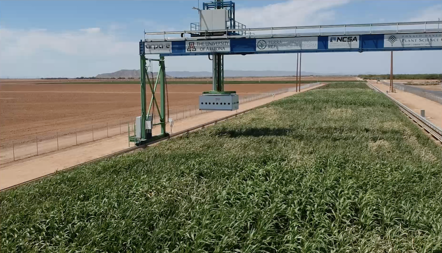
Figure 2: The TERRA-REF Field and Gantry-based Field Scanner in Maricopa, Arizona, with sorghum being grown in the field.

Since 2016, the TERRA-REF platform has collected petabytes of sensor data capturing the full growing cycle of sorghum plants from the sorghum Bioenergy Association Panel [8], a set of 390 sorghum cultivars whose genomes have been fully sequenced and which show promise for bio-energy usage. The full, original TERRA-REF dataset is a massive public domain agricultural dataset, with high spatial and temporal resolution across numerous sensors and seasons, and includes a variety of environmental data and extracted phenotypes in addition to the sensor data. More information about the dataset and access to it can be found in [23].

2.3 Deep Learning for Agriculture

To our knowledge, this is the first work that trains classifiers on visual sensor data to predict whether an image shows organisms with a reference or alternate version of a genetic marker in order to better understand the genotype $\times$ phenotype relationship. There is related work in genomic selection that attempts to predict end-of-season traits like leaf or grain length and crop yield [33, 34] from genetic information. In [25], the most related work to ours, the authors train CNNs to predict quantitative traits from SNPs, and use a visualization approach called saliency maps to highlight the SNPs that most contributed to predicting a particular trait (as opposed to predicting whether a SNP is reference or alternate, and what visual components led to that classification). There is additionally work that attempts to use deep learning to predict the relative functional importance of specific genetic markers and mutations in plants [43], without focusing on visualizing their specific impact on the expressed phenotypes.

There is generally significantly more work in applying deep learning for a wide variety of plant phenotyping and agriculture tasks that do not incorporate the underlying genetics – for example, deep CNNs have successfully been used for fruit detection [40, 32, 22, 4, 24], cultivar and species identification [30, 19, 24, 3, 5, 39, 31], plant disease classification [42, 16, 27, 36, 42], leaf counting [37, 1, 17, 15], yield prediction [26, 29, 41, 12], and stress detection [11, 10, 2], among other phenotyping tasks.

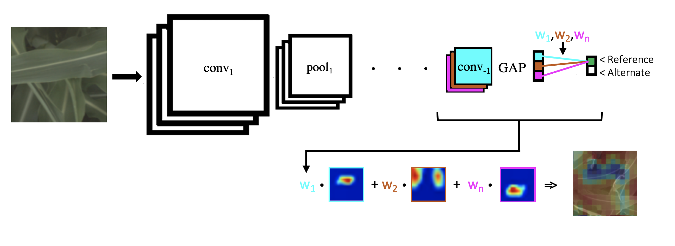
Figure 3: We use a standard ResNet-50 architecture, which like many deep convolutional neural networks consists of alternating convolutional and pooling layers (with interspersed activation functions). The network ends with a final convolutional layer, a global average pooling (GAP) operation, and then a fully connected layer, the output of which is used to make our prediction of whether an image shows a plant with a reference or alternate version of a particular genetic marker. We use the class activation mapping approach described in [47], in which the filters in the last convolutional layer are multiplied by the corresponding weights between the respective layer and the predicted output node. These weighted filters are then added up to produce a heatmap that has its highest values in important regions.

3 Methods

Our approach to gaining understanding about the genotype $\times$ phenotype relationship is to train deep convolutional neural networks to predict whether an image shows a sorghum cultivar with the reference or alternate version of a specific SNP or families of SNPs, and to then visualize what visual features the network focuses on when making that determination. If the classifier can perform well above chance at this classification task, then it is learning something that is significantly correlated with the genetics being considered, and the visualizations can help us glean insights into precisely what those correlations are.

In this paper, we focus on five specific families of genetic markers, as defined in Table 1. Each famility of genetic markers is defined by one or more related SNPs, which have been identified in prior work as having a particular phenotype that is impacted depending on whether the cultivar being grown has the reference or alternate version of the marker. (When grouping multiple SNPs together, we consider a cultivar to be reference if it is reference for all of the SNPs, or alternate if it has any alternate SNPs – this is because even one polymorphism can significantly impact the phenotype being controlled.)

We train a ResNet-50 deep convolutional neural network architecture [18] with a single fully connected layer on the reference vs. alternate classification task. A general overview of this type of network architecture is shown at the top of Figure 3.

For all families of genetic markers, the network is trained on 256 $\times$ 256 pixel RGB images from the TERRA-REF Stereo Top RGB cameras, and optimized using adam [21] with a learning rate of 0.0001 for 20 epochs. For data augmentation, we subtract by dataset channel means and divide by dataset channel standard deviations, and during training we perform random horizontal flips. The 256 $\times$ 256 pixel images extracted by resizing the image on its largest side to 256 and extracting a random crop at training time, and a center crop at testing time. We use imbalanced batch sampling during training to fill 100 image batches with a roughly equal number of reference and alternate images per batch, even if there is an imbalance in the number of reference and alternate images in the training set.

We then use the Class Activation Mapping approach described in [47], which highlights the image regions that most contributed to a classification of the neural network. This approach is visualized in the bottom of Figure 3, where the filters in the last convolutional layer are multiplied by the corresponding weights between the respective layer and the predicted output node. These weighted filters are then added up to produce a heatmap that has its highest values in important regions (e.g., the blue regions in Figure 1). We can then look at the heatmaps for the most confident predictions from a neural network trained on a particular genetic marker family to understand the visual traits that are highly correlated with being either reference or alternate, as in Figures 6 and 7.

Genetic Marker Family	SNP Details
	Chromosome	Gene	Position	Known Controlled Phenotype
Leaf Wax	1	001G269200	51588525	Wax composition [38]
	1	001G269200	51588838
	1	001G269200	51589143
	1	001G269200	51589435
dw	6	006G067700	42805319	Plant height and structure, stem length and internode length [46, 20]
	6	006G067700	42804037
Dry Stalk (d) locus	6	006G147400	50898459	Plant height and structure, and sugar composition [45]
	6	006G147400	50898536
	6	006G147400	50898315
	6	006G147400	50898231
	6	006G147400	50898523
	6	006G147400	50898525
ma	6	006G057866	40312463	Flowering time and maturity [14, 28]
	6	006G004400	2697734
tan	9	009G229800	57040680	Pigmentation and tannin production [44]

Table 1: Details about the genetic marker families of interest. Single nucleotide polymorphisms are grouped by the phenotypes they control, and classification is performed by genetic marker family. Cultivars are defined as reference if they have the reference version of all SNPs on both copies of the chromosomes, and as alternate if they have the alternate version of all SNPs on both copies of the chromosomes (we do not consider heterozygous cultivars).

Genetic Marker Family	# Train Cultivars		# Test Cultivars		# Train Images		# Test Images
	Ref	Alt	Ref	Alt	Ref	Alt	Ref	Alt
Leaf Wax	67	114	34	34	16750	28500	8500	8500
dw	80	105	40	40	20000	26250	10000	10000
Dry Stalk (d) locus	43	127	21	21	10750	31750	5200	5200
ma	21	167	10	10	5250	41750	2500	2500
tan	133	53	27	27	33250	13250	6750	6750

Table 2: Dataset Statistics. Specifics on the numbers of cultivars and images used in the training and testing sets for each of the genetic marker families.

4 Dataset Details

For each family of genetic markers, we select the cultivars within the BAP lines that are either homozygous reference or alternate (ignoring heterozygous cultivars). We determine whether there are more reference or alternate cultivars, and select the minimum to define the number of cultivars that are put into our training and testing sets – the testing set includes half of the cultivars from whichever class has fewer cultivars, and an equal number of the better represented class. There is no overlap between the training and testing cultivars.

Within each testing class, we randomly select the same number of images (the number is limited by whichever cultivar has the fewest images). This guarantees that our testing set is balanced both by number of images per class and number of cultivars per class. All remaining cultivars are put into the training set, without limiting the number of images per cultivar – this allows us to use a large number of training examples, even if there may be imbalance in the number of images per class (reference vs. alternate) or per cultivar. This imbalance is dealt with at training time by an imbalanced sampler per batch, which selects roughly equal numbers of images from the population of reference and alternate examples.

Table 2 shows the exact number of cultivars and images used in the training and testing sets for each genetic marker family. We only consider images from June of 2017, mid-way through the growing season when plants are not too small, exhibiting many of the phenotypes of interest, and not yet lodging (falling over) on top of each other.

5 Results

In Table 3, we show the classification accuracy by image and by cultivar for each of the five genetic marker families of interest. The per image accuracy is simply the average accuracy of predicting whether every image in the test set is correctly labeled as homozygous reference or homozygous alternate. When computing the per cultivar accuracy, we take the mode of all images within a cultivar and use that to make the prediction. We then report the average accuracy over all cultivars. Due to the balancing described in Section 4, random chance on either of these tasks is guaranteed to be 0.5. For each of the genetic markers of interest, our models achieve well above chance accuracy, ranging from between 62.75% accuracy for the dw marker and 68.59% accuracy for the tan marker when considering each individual image. Taking the mode by cultivar provides an average improvement of nearly 20% when compared with considering images individually.

Genetic Marker Family	Classification Accuracy
	Per Image	Per Cultivar
Leaf Wax	.6325	0.7647
dw	.6275	0.8375
Dry Stalk (d) locus	.6743	0.8333
ma	.6565	0.8500
tan	.6859	0.8519

Table 3: Classification Accuracy by Image and by Cultivar. Accuracy by image is computed on each image in the test set separately. Accuracy by cultivar is computed by taking the mode of the image predictions from each cultivar. The test set for each genetic marker family is balanced such that the classification accuracy by both image and by cultivar are 0.5.

We additionally show the accuracy on each day in June in Figure 4. There is a slight trend across all of the markers showing slightly improved performance towards the middle of the month, with performance degrading significantly at the end of the month. This is likely explained by the phenotypes of interest being better expressed during this time and therefore being more recognizable, while the end of season degradation may be related to lodging that happens as the season progresses, where plants in adjacent plots start falling over into each other.

In Figures 6 and 7, we show 15 of the most confident and correctly predicted reference and alternate images and their corresponding heatmaps for each of the genetic markers. These visualizations provide compelling insights into what the networks have learned to focus on, and therefore what visual plant features are highly correlated with a plant either being reference or alternate for a particular genetic marker. In the following paragraphs, we will discuss notable observations from these visualizations and how they correspond to the phenotypes these markers are known to control. In all visualizations, blue regions indicate visual features that are more important for the classification, while red regions are less important.

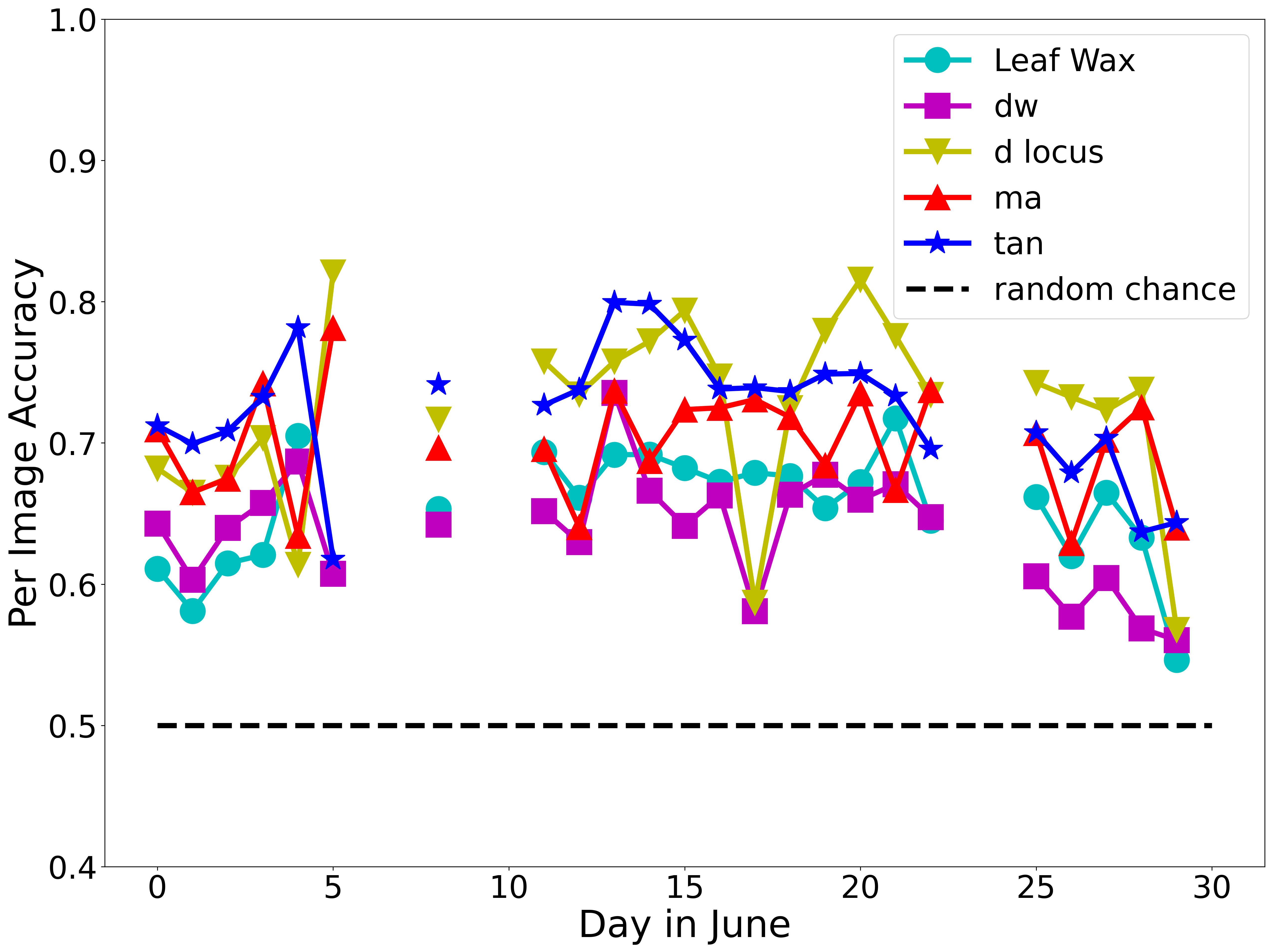
Figure 4: Genetic Marker Family classification accuracy by date. Here we show the accuracy per image for each genetic marker family on each day in June (mid-way through the growing season). In general performance is slightly better in the middle of the month, and worse at the end of the month when plants begin to lodge.

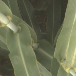
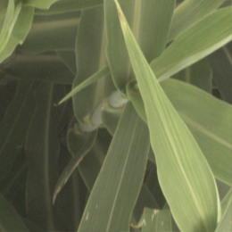
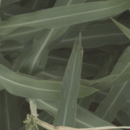
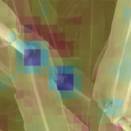
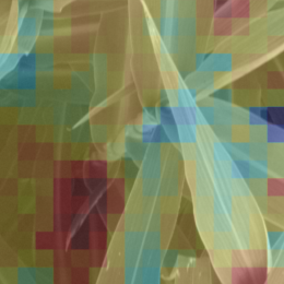
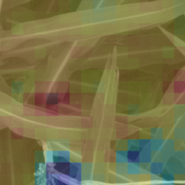
Figure 5: One of the features the neural network trained on the leaf wax SNPs learned to focus on when classifying an image as “reference” was the interface between the stem and either leaves or panicles. Field biologists who reviewed these visualizations were excited to see this feature highlighted, as this is often the feature they look at in the field as it’s where wax build up is most obvious.

In Figure 6(a), we show the most confident correct predictions for the leaf wax genetic marker family. Cultivars with the reference version of these SNPs are known to be more waxy, while the alternate versions are less waxy. In the reference heat maps, the important (blue) regions are often diffuse, covering much of the leaf, while the alternate visualizations are very focused on the spine of the leaf. Looking at the images, it is apparent that in the alternate images, this spine is more brightly differentiated from the rest of the leaf, while in the reference images the spine has less contrast. This corresponds to the wax build up on the leaf in the reference images, which cause the overall leaf to be whiter, resulting in lower contrast on the spine. When the reference visualizations are not diffuse, they focus specifically on the interface between the sorghum plant spine and leaf – this is shown in greater detail in Figure 5. When reviewing these visualizations with a biologist on our team that does in-field ground truth phenotyping of traits including leaf wax, they said: “That’s exactly the place I look at when determining waxiness in the field – it’s where there’s the wax is most obvious!” Excitingly, this indicates that the network has learned, without explicit direction, to focus on the same plant parts as expert humans.

In Figures 6(b and c) and 7(d), the alternate visualizations appear to frequently focus on particular panicles at different growth stages (the panicles focused on for the dw and ma genetic markers are earlier in their life cycle when compared to the panicles in the d locus visualizations). This corresponds to the knowledge that polymorphisms in these genetic markers control features like plant growth rate (SNPs in the dw and dlocus families are considered ‘drawfing’ markers, controling growth rate and ultimate plant height), flowering time and maturity. The d locus reference visualizations also appear to focus on particular leaf shapes – the ends of broad leaves – which similarly may relate to the fact that the markers are known to exhibit control over plant structure.

In Figure 7(e), we show the confident images and heatmaps for the tan SNP, which controls tannin production and pigmentation. Notably, plants with the reference version of the SNP are known to have less tannin production, resulting in a less bitter taste in the plant seeds. This is interestingly manifested in the reference visualizations which highlight panicles where all of the seeds have been eaten – likely because they taste better to birds!

(a) Leaf Wax
Reference
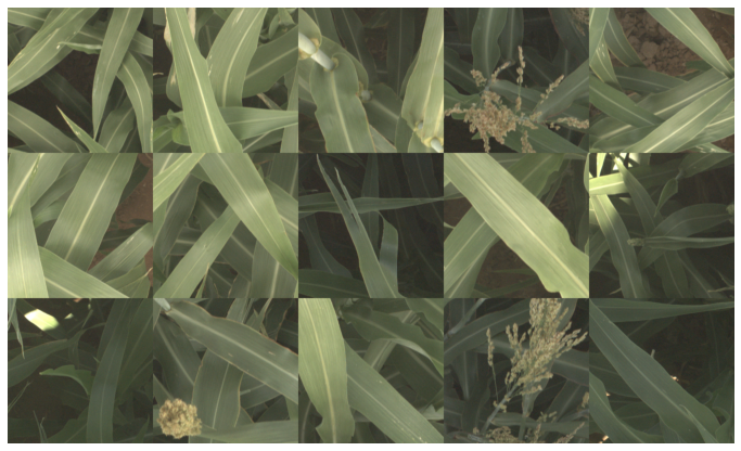
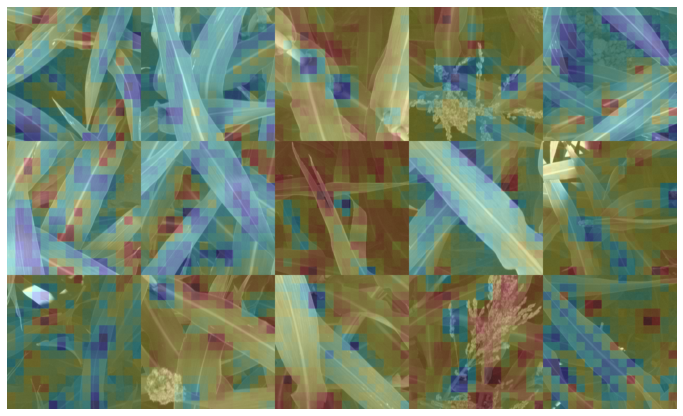
Alternate
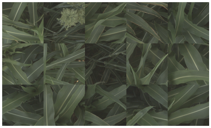
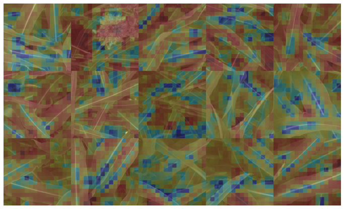
(b) dw
Reference
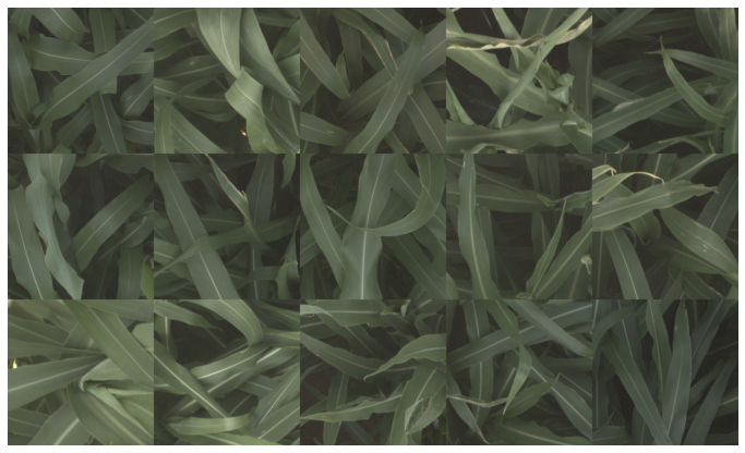
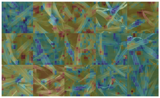
Alternate
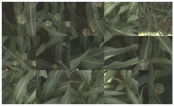
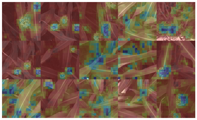
(c) Dry Stalk (d) Locus
Reference
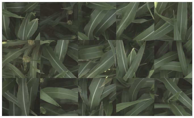
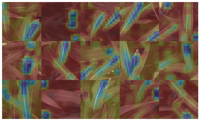
Alternate

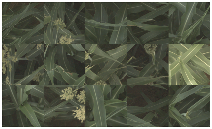
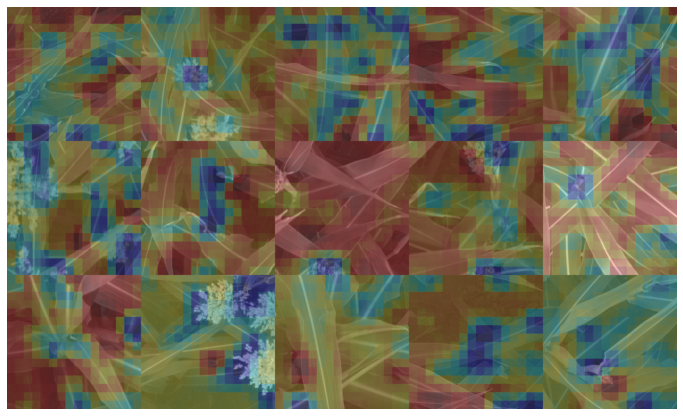
Figure 6: Confident and correct examples for the classification of leaf wax, dw and d locus genetic markers. Blue regions are important to the prediction, while red regions are less important or even detract from the prediction.

(d) ma
Reference
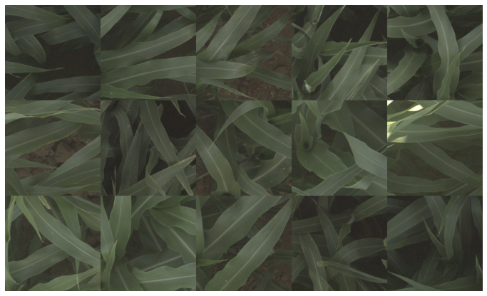
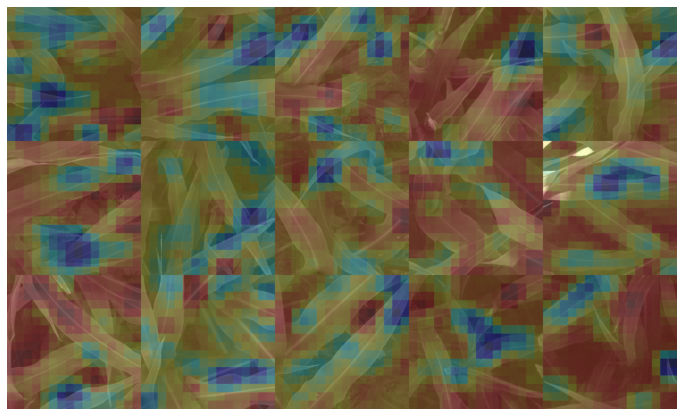
Alternate
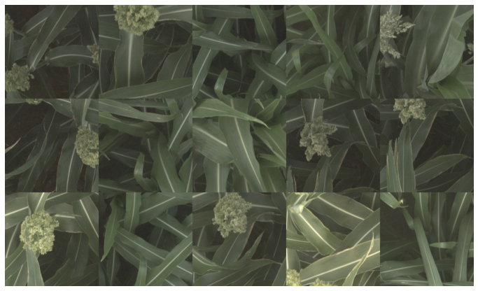
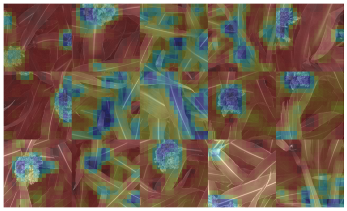
(e) tan
Reference
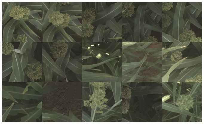
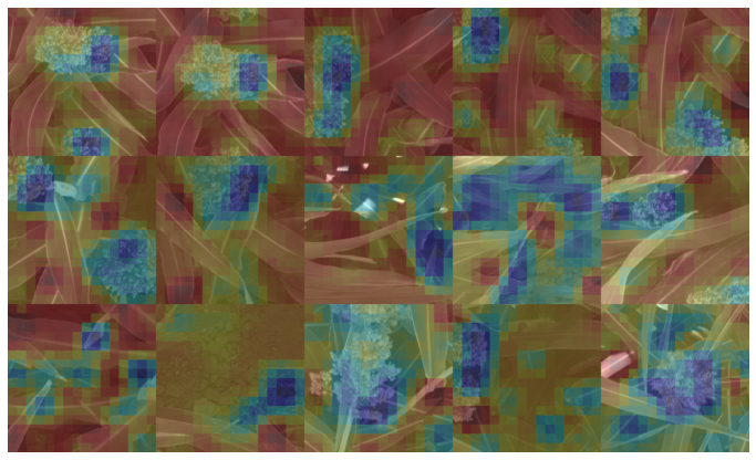
Alternate

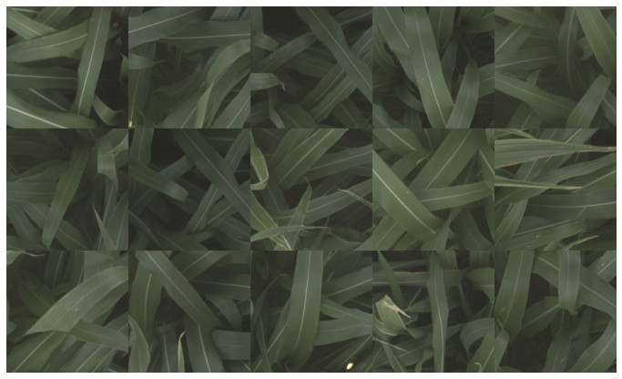
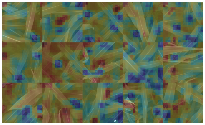
Figure 7: Confident and correct examples for the classification of ma and tan genetic markers. Blue regions are important to the prediction, while red regions are less important or even detract from the prediction.

6 Conclusions & Future Work

In this paper, we demonstrated the feasibility of a pipeline to help understand the genotype $\times$ phenotype relationship in sorghum by training deep convolutional neural networks on visual sensor data to predict whether different crops have reference or alternate versions of particular genetic markers. We show for several genetic markers that whose phenotypic expression is well understood that these networks can achieve well-above chance performance on this task, and that visualizations that highlight the most important parts of the images that led to the classification correspond with the known phenotypes.

This approach can be extended to not only help better understand well-established genotype $\times$ phenotype relationships, but to explore new, less well understood relationships. The same approach could be deployed for SNPs and families of SNPs whose phenotypic expression is not understood, to uncover new and interesting polymorphisms.

This paper presented a very simple, yet effective pipeline, focused on a relatively limited time period of high resolution data from the TERRA-REF gantry system (data from the entire month of June, mid-way through the growing season in 2017). We recognize that not all phenotypes, however, are observable during this time period. Especially when considering unknown genetic markers, it may be beneficial to consider longer time periods including both early and late growing periods when different phenotypes are expressed. This is a direction for future work: longer time periods may require more complex training protocols that more explicitly incorporate time – for example, using recurrent approaches, or training a multi-headed network that simultaneously predicts the genetic class and the date. Additional work could focus on extending the approach to sensors other than RGB cameras, as some phenotypes may be more readily observed in different sensing modalities, such as hyperspectral or thermal imagery, or in the structural information from the 3D laser scanner.

References

- [1] Shubhra Aich and Ian Stavness. Leaf counting with deep convolutional and deconvolutional networks. In Proceedings of the IEEE International Conference on Computer Vision Workshops, pages 2080–2089, 2017.
- [2] Basavaraj S Anami, Naveen N Malvade, and Surendra Palaiah. Deep learning approach for recognition and classification of yield affecting paddy crop stresses using field images. Artificial Intelligence in Agriculture, 4:12–20, 2020.
- [3] Belal AM Ashqar, Bassem S Abu-Nasser, and Samy S Abu-Naser. Plant seedlings classification using deep learning. 2019.
- [4] Suchet Bargoti and James Underwood. Deep fruit detection in orchards. In 2017 IEEE International Conference on Robotics and Automation (ICRA), pages 3626–3633. IEEE, 2017.
- [5] Pierre Barré, Ben C Stöver, Kai F Müller, and Volker Steinhage. Leafnet: A computer vision system for automatic plant species identification. Ecological Informatics, 40:50–56, 2017.
- [6] Barry R Bochner. New technologies to assess genotype–phenotype relationships. Nature Reviews Genetics, 4(4):309–314, 2003.
- [7] Richard E Boyles, Zachary W Brenton, and Stephen Kresovich. Genetic and genomic resources of sorghum to connect genotype with phenotype in contrasting environments. The Plant Journal, 97(1):19–39, 2019.
- [8] Zachary W Brenton, Elizabeth A Cooper, Mathew T Myers, Richard E Boyles, Nadia Shakoor, Kelsey J Zielinski, Bradley L Rauh, William C Bridges, Geoffrey P Morris, and Stephen Kresovich. A genomic resource for the development, improvement, and exploitation of sorghum for bioenergy. Genetics, 204(1):21–33, 2016.
- [9] Maxwell Burnette, Rob Kooper, J. D. Maloney, Gareth S. Rohde, Jeffrey A. Terstriep, Craig Willis, Noah Fahlgren, Todd Mockler, Maria Newcomb, Vasit Sagan, Pedro Andrade-Sanchez, Nadia Shakoor, Paheding Sidike, Rick Ward, and David LeBauer. TERRA-REF data processing infrastructure. In Sergiu Sanielevici, editor, Proceedings of the Practice and Experience on Advanced Research Computing, PEARC 2018, Pittsburgh, PA, USA, July 22-26, 2018, pages 27:1–27:7. ACM, 2018.
- [10] Sujata Butte, Aleksandar Vakanski, Kasia Duellman, Haotian Wang, and Amin Mirkouei. Potato crop stress identification in aerial images using deep learning-based object detection. arXiv preprint arXiv:2106.07770, 2021.
- [11] Narendra Singh Chandel, Subir Kumar Chakraborty, Yogesh Anand Rajwade, Kumkum Dubey, Mukesh K Tiwari, and Dilip Jat. Identifying crop water stress using deep learning models. Neural Computing and Applications, 33(10):5353–5367, 2021.
- [12] Yang Chen, Won Suk Lee, Hao Gan, Natalia Peres, Clyde Fraisse, Yanchao Zhang, and Yong He. Strawberry yield prediction based on a deep neural network using high-resolution aerial orthoimages. Remote Sensing, 11(13):1584, 2019.
- [13] Joshua N Cobb, Genevieve DeClerck, Anthony Greenberg, Randy Clark, and Susan McCouch. Next-generation phenotyping: requirements and strategies for enhancing our understanding of genotype–phenotype relationships and its relevance to crop improvement. Theoretical and Applied Genetics, 126(4):867–887, 2013.
- [14] Hugo E. Cuevas, Chengbo Zhou, Haibao Tang, Prashant P. Khadke, Sayan Das, Yann-Rong Lin, Zhengxiang Ge, Thomas Clemente, Hari D. Upadhyaya, C. Thomas Hash, and Andrew H. Paterson. The Evolution of Photoperiod-Insensitive Flowering in Sorghum, A Genomic Model for Panicoid Grasses. Molecular Biology and Evolution, 33(9):2417–2428, 06 2016.
- [15] Andrei Dobrescu, Mario Valerio Giuffrida, and Sotirios A Tsaftaris. Leveraging multiple datasets for deep leaf counting. In Proceedings of the IEEE International Conference on Computer Vision Workshops, pages 2072–2079, 2017.
- [16] Konstantinos P Ferentinos. Deep learning models for plant disease detection and diagnosis. Computers and Electronics in Agriculture, 145:311–318, 2018.
- [17] Mario Valerio Giuffrida, Peter Doerner, and Sotirios A Tsaftaris. Pheno-deep counter: A unified and versatile deep learning architecture for leaf counting. The Plant Journal, 96(4):880–890, 2018.
- [18] Kaiming He, Xiangyu Zhang, Shaoqing Ren, and Jian Sun. Deep residual learning for image recognition. IEEE Conference on Computer Vision and Pattern Recognition (CVPR), pages 770–778, 2016.
- [19] Ahmad Heidary-Sharifabad, Mohsen Sardari Zarchi, Sima Emadi, and Gholamreza Zarei. An efficient deep learning model for cultivar identification of a pistachio tree. British Food Journal, 2021.
- [20] Josie L. Hilley, Brock D. Weers, Sandra K. Truong, Ryan F. McCormick, Ashley J. Mattison, Brian A. McKinley, Daryl T. Morishige, and John E. Mullet. Sorghum dw2 encodes a protein kinase regulator of stem internode length. Scientific Reports, 7(1), 7 2017.
- [21] Diederik P. Kingma and Jimmy Ba. Adam: A method for stochastic optimization. In Yoshua Bengio and Yann LeCun, editors, 3rd International Conference on Learning Representations, ICLR 2015, San Diego, CA, USA, May 7-9, 2015, Conference Track Proceedings, 2015.
- [22] Anand Koirala, KB Walsh, Zhenglin Wang, and C McCarthy. Deep learning for real-time fruit detection and orchard fruit load estimation: Benchmarking of ‘mangoyolo’. Precision Agriculture, 20(6):1107–1135, 2019.
- [23] David LeBauer, Maxwell A. Burnette, Jeffrey Demieville, Noah Fahlgren, Andrew N. French, Roman Garnett, Zhenbin Hu, Kimberly Huynh, Rob Kooper, Zongyang Li, Maitiniyazi Maimaitijiang, Jerome Mao, Todd C. Mockler, Geoffrey Morris, Maria Newcomb, Michael J Ottman, Philip Ozersky, Sidike Paheding, Duke Pauli, Robert Pless, Wei Qin, Kristina Riemer, Gareth Scott Rohde, William L. Rooney, Vasit Sagan, Nadia Shakoor, Abby Stylianou, Kelly Thorp, Richard Ward, Jeffrey W White, Craig Willis, and Charles S Zender. TERRA-REF, An Open Reference Data Set From High Resolution Genomics, Phenomics, and Imaging Sensors. https://datadryad.org/stash/dataset/doi:10.5061/dryad.4b8gtht99, 2020.
- [24] Marcus Guozong Lim and Joon Huang Chuah. Durian types recognition using deep learning techniques. In 2018 9th IEEE Control and System Graduate Research Colloquium (ICSGRC), pages 183–187. IEEE, 2018.
- [25] Yang Liu, Duolin Wang, Fei He, Juexin Wang, Trupti Joshi, and Dong Xu. Phenotype prediction and genome-wide association study using deep convolutional neural network of soybean. Frontiers in genetics, 10:1091, 2019.
- [26] Maitiniyazi Maimaitijiang, Vasit Sagan, Paheding Sidike, Sean Hartling, Flavio Esposito, and Felix B Fritschi. Soybean yield prediction from uav using multimodal data fusion and deep learning. Remote Sensing of Environment, 237:111599, 2020.
- [27] Sharada P Mohanty, David P Hughes, and Marcel Salathé. Using deep learning for image-based plant disease detection. Frontiers in plant science, 7:1419, 2016.
- [28] Rebecca L. Murphy, Daryl T. Morishige, Jeff A. Brady, William L. Rooney, Shanshan Yang, Patricia E. Klein, and John E. Mullet. Ghd7 (ma6) represses sorghum flowering in long days: Ghd7 alleles enhance biomass accumulation and grain production. The Plant Genome, 7(2):plantgenome2013.11.0040, 2014.
- [29] Petteri Nevavuori, Nathaniel Narra, and Tarmo Lipping. Crop yield prediction with deep convolutional neural networks. Computers and electronics in agriculture, 163:104859, 2019.
- [30] Yutaro Osako, Hisayo Yamane, Shu-Yen Lin, Po-An Chen, and Ryutaro Tao. Cultivar discrimination of litchi fruit images using deep learning. Scientia Horticulturae, 269:109360, 2020.
- [31] C. Ren, Justin Dulay, Gregory Rolwes, D. Pauli, N. Shakoor, and Abby Stylianou. Multi-resolution outlier pooling for sorghum classification. Agriculture-Vision Workshop in IEEE/CVF Conference on Computer Vision and Pattern Recognition Workshops (CVPRW), 2021.
- [32] Inkyu Sa, Zongyuan Ge, Feras Dayoub, Ben Upcroft, Tristan Perez, and Chris McCool. Deepfruits: A fruit detection system using deep neural networks. sensors, 16(8):1222, 2016.
- [33] Karansher S. Sandhu, Dennis N. Lozada, Zhiwu Zhang, Michael O. Pumphrey, and Arron H. Carter. Deep learning for predicting complex traits in spring wheat breeding program. Frontiers in Plant Science, 11:2084, 2021.
- [34] Karansher S. Sandhu, Dennis N. Lozada, Zhiwu Zhang, Michael O. Pumphrey, and Arron H. Carter. Deep learning for predicting complex traits in spring wheat breeding program. Frontiers in Plant Science, 11:2084, 2021.
- [35] Jennifer A Schweitzer, Joseph K Bailey, Dylan G Fischer, Carri J LeRoy, Eric V Lonsdorf, Thomas G Whitham, and Stephen C Hart. Plant–soil–microorganism interactions: heritable relationship between plant genotype and associated soil microorganisms. Ecology, 89(3):773–781, 2008.
- [36] Edna Chebet Too, Li Yujian, Sam Njuki, and Liu Yingchun. A comparative study of fine-tuning deep learning models for plant disease identification. Computers and Electronics in Agriculture, 161:272–279, 2019.
- [37] Jordan Ubbens, Mikolaj Cieslak, Przemyslaw Prusinkiewicz, and Ian Stavness. The use of plant models in deep learning: an application to leaf counting in rosette plants. Plant methods, 14(1):1–10, 2018.
- [38] Anurag Uttam, Praveen Madgula, Yechuri Rao, Vilas Tonapi, and Ragimasalawada Madhusudhana. Molecular mapping and candidate gene analysis of a new epicuticular wax locus in sorghum (sorghum bicolor l. moench). Theoretical and Applied Genetics, 130, 10 2017.
- [39] Grant Van Horn, Oisin Mac Aodha, Yang Song, Yin Cui, Chen Sun, Alex Shepard, Hartwig Adam, Pietro Perona, and Serge Belongie. The inaturalist species classification and detection dataset. In Proceedings of the IEEE conference on computer vision and pattern recognition, pages 8769–8778, 2018.
- [40] Shaohua Wan and Sotirios Goudos. Faster r-cnn for multi-class fruit detection using a robotic vision system. Computer Networks, 168:107036, 2020.
- [41] Anna X Wang, Caelin Tran, Nikhil Desai, David Lobell, and Stefano Ermon. Deep transfer learning for crop yield prediction with remote sensing data. In Proceedings of the 1st ACM SIGCAS Conference on Computing and Sustainable Societies, pages 1–5, 2018.
- [42] Guan Wang, Yu Sun, and Jianxin Wang. Automatic image-based plant disease severity estimation using deep learning. Computational intelligence and neuroscience, 2017, 2017.
- [43] Hai Wang, Emre Cimen, Nisha Singh, and Edward Buckler. Deep learning for plant genomics and crop improvement. Current Opinion in Plant Biology, 54:34–41, 2020. Genome studies and molecular genetics.
- [44] Yuye Wu, Xianran Li, Wenwen Xiang, Chengsong Zhu, Zhongwei Lin, Yun Wu, Jiarui Li, Satchidanand Pandravada, Dustan D. Ridder, Guihua Bai, Ming L. Wang, Harold N. Trick, Scott R. Bean, Mitchell R. Tuinstra, Tesfaye T. Tesso, and Jianming Yu. Presence of tannins in sorghum grains is conditioned by different natural alleles of tannin1. Proceedings of the National Academy of Sciences, 109(26):10281–10286, 2012.
- [45] Jingnu Xia, Yunjun Zhao, Payne Burks, Markus Pauly, and Patrick J. Brown. A sorghum nac gene is associated with variation in biomass properties and yield potential. Plant Direct, 2(7):e00070, 2018.
- [46] Miki Yamaguchi, Haruka Fujimoto, Ko Hirano, Satoko Araki-Nakamura, Kozue Ohmae-Shinohara, Akihiro Fujii, Masako Tsunashima, Xian Song, Yusuke Ito, Rie Nagae, Jianzhong wu, Hiroshi Mizuno, Jun-Ichi Yonemaru, Takashi Matsumoto, Hidemi Kitano, Makoto Matsuoka, Shigemitsu Kasuga, and Takashi Sazuka. Sorghum dw1, an agronomically important gene for lodging resistance, encodes a novel protein involved in cell proliferation. Scientific Reports, 6:28366, 06 2016.
- [47] B. Zhou, A. Khosla, Lapedriza. A., A. Oliva, and A. Torralba. Learning Deep Features for Discriminative Localization. CVPR, 2016.