Mixture of Linear Models Co-supervised by Deep Neural Networks

Abstract

Deep neural networks (DNN) have been demonstrated to achieve unparalleled prediction accuracy in a wide range of applications. Despite its strong performance, in certain areas, the usage of DNN has met resistance because of its black-box nature. In this paper, we propose a new method to estimate a mixture of linear models (MLM) for regression or classification that is relatively easy to interpret. We use DNN as a proxy of the optimal prediction function such that MLM can be effectively estimated. We propose visualization methods and quantitative approaches to interpret the predictor by MLM. Experiments show that the new method allows us to trade-off interpretability and accuracy. The MLM estimated under the guidance of a trained DNN fills the gap between a highly explainable linear statistical model and a highly accurate but difficult to interpret predictor.

Keywords: Explainable machine learning, DNN co-supervision, Explainable dimensions, Explainable conditions, Interpretation of DNN

1 Introduction

Deep neural network (DNN) models have achieved phenomenal success for applications in many domains, ranging from academic research in science and engineering to industry and business. The modeling power of DNN is believed to have come from the complexity and over-parameterization of the model, which on the other hand has been criticized for the lack of interpretation. Although certainly not true for every application, in some applications, especially in economics, social science, healthcare industry, and administrative decision making, scientists or practitioners are resistant to use predictions made by a black-box system for multiple reasons. One reason is that a major purpose of a study can be to make discoveries based upon the prediction function, e.g., to reveal the relationships between measurements. Another reason can be that the training dataset is not large enough to make researchers feel completely sure about a purely data-driven result. Being able to examine and interpret the prediction function will enable researchers to connect the result with existing knowledge or gain insights about new directions to explore. Although classic statistical models are much more explainable, their accuracy often falls considerably below DNN. In this paper, we propose an approach to fill the gap between relatively simple explainable models and DNN such that we can more flexibly tune the trade-off between interpretability and accuracy. Our main idea is a mixture of discriminative models that is trained with the guidance from a DNN. Although mixtures of discriminative models have been studied before, our way of generating the mixture is quite different.

1.1 Related Work

Despite the fact that many attempts have been made to make DNN models more interpretable, a formal definition of “human interpretability” has remained elusive. The concept of interpretability is multifaceted and inevitably subjective. An in-depth discussion about the meaning of being interpretable is given by the review article of Doshi-Velez and Kim, (2017), which confirms the richness of this concept and provides philosophical viewpoints. In the literature, different approaches have been proposed to define “interpretation”. A complete unified taxonomy for all the existing approaches does not exist. Nevertheless, one way is to categorize recent works into two types: one that builds more interpretable models by reducing model complexity, and the other that attempts to interpret a complex model by examining certain aspects of it, e.g., how decisions are made locally. For the first type of approaches, interpretability is aimed at during the model’s training phase, and what constitutes good interpretability has been addressed in diverse ways. For example, attention-based methods (Bahdanau et al.,, 2014; Vaswani et al.,, 2017) propose an attention score for neural machine translation; generalized additive models (GAM) (Lou et al.,, 2013; Agarwal et al.,, 2020; Guo et al.,, 2020) interpret pair-wise interaction effects by imposing an additive structure; and feature selection methods impose cross-entropy error function (Verikas and Bacauskiene,, 2002) or $L_{0}$ penalization (Tsang et al.,, 2018). In contrast, the second type of approaches, the so-called model-agnostic methods (Ribeiro et al., 2016b, ), are post-hoc in the sense that they analyze an already trained model using interpretable measurements. For example, sensitivity analysis (Lundberg and Lee,, 2017), local linear surrogate models (Ribeiro et al., 2016a, ) and Bayesian non-parametric mixture model (Guo et al.,, 2018) search for important features for specific samples according to a given prediction model. The same aspect of being interpretable can be tackled by either type of the approaches. For example, Tsang et al., (2017) searches for interaction effects of original features as captured in a trained neural network by computing a strength score based on the learned weights. In Tsang et al., (2018), similar results can be obtained by training the neural network model with a penalty to learn the interaction effects.

Various kinds of interpretation have been suggested, including but not limited to visualizing the result, generating human explainable rules, selecting features, or constructing prototype cases. The advantages and disadvantages of existing methods are discussed in detail in Molnar, (2020). What forms of interpretation are valuable also depends on the field of applications. For instance, feature selection for image processing may not be as meaningful as that for tabular data. Many proposed methods target particular applications, e.g., image processing (Zhang et al.,, 2018; Chen et al.,, 2019), text mining (Vaswani et al.,, 2017), time series (Guo et al.,, 2019).

Ribeiro et al., 2016a interprets neural networks by explaining how the decision is made in the vicinity of every instance. In particular, the trained neural network is used to generate pairs of input and output quantities, based on which a linear regression model is estimated. This linear model is used to explain the decision in the neighborhood of that instance. Although the local linear models help understand the prediction around every single point, they are far from providing global perspectives. Our new method is inspired by Ribeiro et al., 2016a , but we tackle two additional problems. First, our method will produce a stand-alone prediction model that is relatively easy to interpret. In another word, our method is not the model-agnostic type to explain an actual operating DNN. Second, our method aims at globally interpreting the decision.

Although motivated from rather different aspects, in terms of the formulation of the model, our method is related to locally weighted regression (Cleveland and Devlin,, 1988) which splits the space of the original independent variables by a user-specified bandwidth and estimates a local linear regression inside each band. In non-parametric regression, many other flexible regression models have been studied, for instance, kernel regression (Nadaraya,, 1964; Watson,, 1964), generalized additive models (Hastie and Tibshirani,, 1990), and classification and regression trees (CART) (Breiman et al.,, 1984). Some of the methods such as CART are by construction highly interpretable, but some are not. More recently, Guo et al., (2020) have used neural networks to efficiently learn the classic GAM (Hastie and Tibshirani,, 1990) models.

1.2 Overview of Our Approach

One natural idea to explain a complex model is to view the decision as a composite of decisions made by different functions in different regions of the input space. Explanation of the overall model consists of two parts: to explain how the partition of the input space is formed, and to explain the prediction in each region. This idea points to the construction of a mixture model in which every component is a linear model, which is called the mixture of linear models (MLM). Although a linear model is not necessarily always easy to explain, relatively speaking, it is explainable, and via LASSO-type sparsity penalty (Tibshirani,, 1996) it can be made increasingly more explainable. Moreover, well-studied hypothesis testing can be applied to validate the model.

The main technical hurdle is to find a suitable partition of the instances such that component-wise linear models can be estimated. The challenge faced here is in stark contrast to that for building generative mixture models, e.g., Gaussian mixture models (GMM), where the proximity of the independent variables themselves roughly determines the grouping of instances into components. The same approach of forming components is a poor choice for building a mixture of discriminative models. The similarity between the instances is no longer measured by the proximity of the independent variables but by the proximity of the relationships between the dependent variable ($Y$) and the independent variables ($X$). However, the dependence between $Y$ and $X$ cannot be adequately captured by the observation of one instance. In the case of moderate to high dimensions, it is also impractical to estimate the discriminative function, $\hat{Y}=f(X)$, based on nearby points. Our key idea is to use the DNN model as an approximation of the theoretically optimal prediction function, which is employed to guide the partition of the instances. We also propose to use visualization based on GMM and decision tree to interpret the partition of the instances, which is crucial for obtaining interpretation in a global sense.

It is debatable whether DNN serves well as an approximation of the optimal prediction function. In many applications, we observe that DNN achieves the best accuracy among the state-of-the-art methods, e.g., support vector machine (SVM) (Cortes and Vapnik,, 1995) and random forest (RF) (Breiman,, 2001). It is thus reasonable to exploit DNN in this manner. However, we acknowledge that a weakness of our approach is that the accuracy is mostly capped by DNN, and if DNN itself performs inferior, the same is likely to occur with our approach.

The rest of the paper is organized as follows. In Section 2, we introduce notations and summarize existing methods most relevant to our proposed work. We present MLM in Section 3.1 and describe the tools developed for interpretation based upon MLM in Section 3.2. In Section 4, experimental results are reported for four real-world datasets including two clinical datasets for classification and two for regression. For prediction accuracy, comparisons have been made with multiple approaches including DNN. We also illustrate how the interpretation tools are used. Finally, conclusions are drawn in Section 5.

2 Preliminaries

Let $X\in\mathbb{R}^{p}$ be the independent variables (or covariates) and $Y\in\mathbb{R}$ be the dependent variable. Denote the sample space of $X$ by $\mathcal{X}$. Let $\{y_{i}\}_{i=1}^{n}$ and $\{\mathbf{x}_{i}\}_{i=1}^{n}=\{(x_{i,1},\cdots,x_{i,p})^{T}\}_{i=1}^{n}$ be the $n$ observations of $Y$ and $X$. Denote the input data matrix by $\mathbf{X}\in\mathbb{R}^{n\times p}$. In regression analysis, we are interested in estimating the following regression function for any $\mathbf{x}\in\mathcal{X}$ (for classification, we simply substitute $Y$ by $g(Y)$ via a link function $g(\cdot)$).

$$m(\mathbf{x})=\mathbb{E}(Y|X=\mathbf{x})\;.$$ (1)

In linear regression, it is assumed that $m(\mathbf{x})=\alpha+\mathbf{x}^{T}\mathbf{\beta}$. In non-linear regression, a linear expansion of basis functions is often used to estimate $m(\mathbf{x})$. For example, Nadaraya-Watson kernel regression (Nadaraya,, 1964; Watson,, 1964) assumes $m(\mathbf{x})$ to be an additive form of kernel functions with a given bandwidth $h$:

$$m(\mathbf{x})=\sum\limits_{i=1}^{n}\frac{G(\frac{\mathbf{x}-\mathbf{x}_{i}}{h})y_{i}}{\sum\limits_{i^{\prime}=1}^{n}G(\frac{\mathbf{x}-\mathbf{x}_{i^{\prime}}}{h})}\,,$$ (2)

where $G(\mathbf{x})=(2\pi)^{-k/2}e^{-\mathbf{x}^{T}\mathbf{x}/2}$. The locally weighted regression (Cleveland and Devlin,, 1988) extends Nadaraya-Watson’s $m(\mathbf{x})$ by changing the constant prediction in each band to a linear function. Regression splines use piecewise polynomial basis functions between fixed points, known as knots, and ensure smoothness at the knots (Schoenberg,, 1973). Friedman, (1991) extended the spline method so as to handle higher dimensional data. These kernel and spline-based approaches use the basic binning strategy to separate the covariate space into regions, which suffers from curse of dimensionality even at moderate dimensions.

In recent years, DNN has become increasingly popular in high-dimensional applications because of its remarkable prediction accuracy. Consider a feed-forward neural network with $L$ hidden layers and one output layer. Its regression function, denoted by $\widetilde{m}(\mathbf{x})$, is defined by the composition of the affine transform and a non-linear activation function at each layer. Let $p_{l}$ be the number of hidden units at the $l$-th hidden layer, $l=0,...,L$, and $p_{0}=p$. Let $\mathbf{z}^{(l)}\in\mathbb{R}^{p_{l}}$ be the outputs of the $l$th hidden layer. Set $\mathbf{z}^{(0)}=\mathbf{x}$. The mapping at the $l$-th hidden layer, $\mathbf{z}^{(l)}=h_{l}(\mathbf{z}^{(l-1)})$, is defined by

$$\mathbf{z}^{(l)} = h_{l}(\mathbf{z}^{(l-1)})$$ (3)

$$= \sigma_{l}(\mathbf{W}^{(l)}\mathbf{z}^{(l-1)}+\mathbf{b}^{(l)}),\;\;l=1,\cdots,L,$$

where $\sigma_{l}(\cdot)$ is a non-linear element-wise activation function such as ReLU (Nair and Hinton,, 2010), sigmoid or hyperbolic tangent, and $\mathbf{W}^{(l)}\in\mathbb{R}^{p_{l}\times p_{l-1}}$ and $\mathbf{b}^{(l)}\in\mathbb{R}^{p_{l}}$ are the model parameters. At the output layer, $g(\mathbf{z}^{(L)})$, is defined as either a linear or softmax function depending on whether the purpose is regression or classification. In summary, the neural network model, $\widetilde{m}(\mathbf{x})$, is given by

$$\widetilde{m}(\mathbf{x})=(g\circ h_{L}\circ h_{L-1}\circ\cdots\circ h_{1})(\mathbf{x}),$$ (4)

and its parameters are trained by gradient descent algorithm so that the mean squared error loss for regression or the cross-entropy loss for classification is minimized. Specifically, the mean squared error loss is defined by

$$\sum\limits_{i=1}^{n}\left[y_{i}-\widetilde{m}(\mathbf{x}_{i})\right]^{2}/n\,,$$

and the cross-entropy loss is

$$-\sum\limits_{i=1}^{n}\left[y_{i}\log(\widetilde{m}(\mathbf{x}_{i}))+(1-y_{i})\log(1-\widetilde{m}(\mathbf{x}_{i}))\right]/n.$$

Because of the multiple layers and the large number of hidden units at every layer, it is difficult to interpret a DNN model, for example, to explain the effects of the input variables on the predicted variable.

3 Methods

Figure 1: A schematic plot showing the steps of creating MLM.

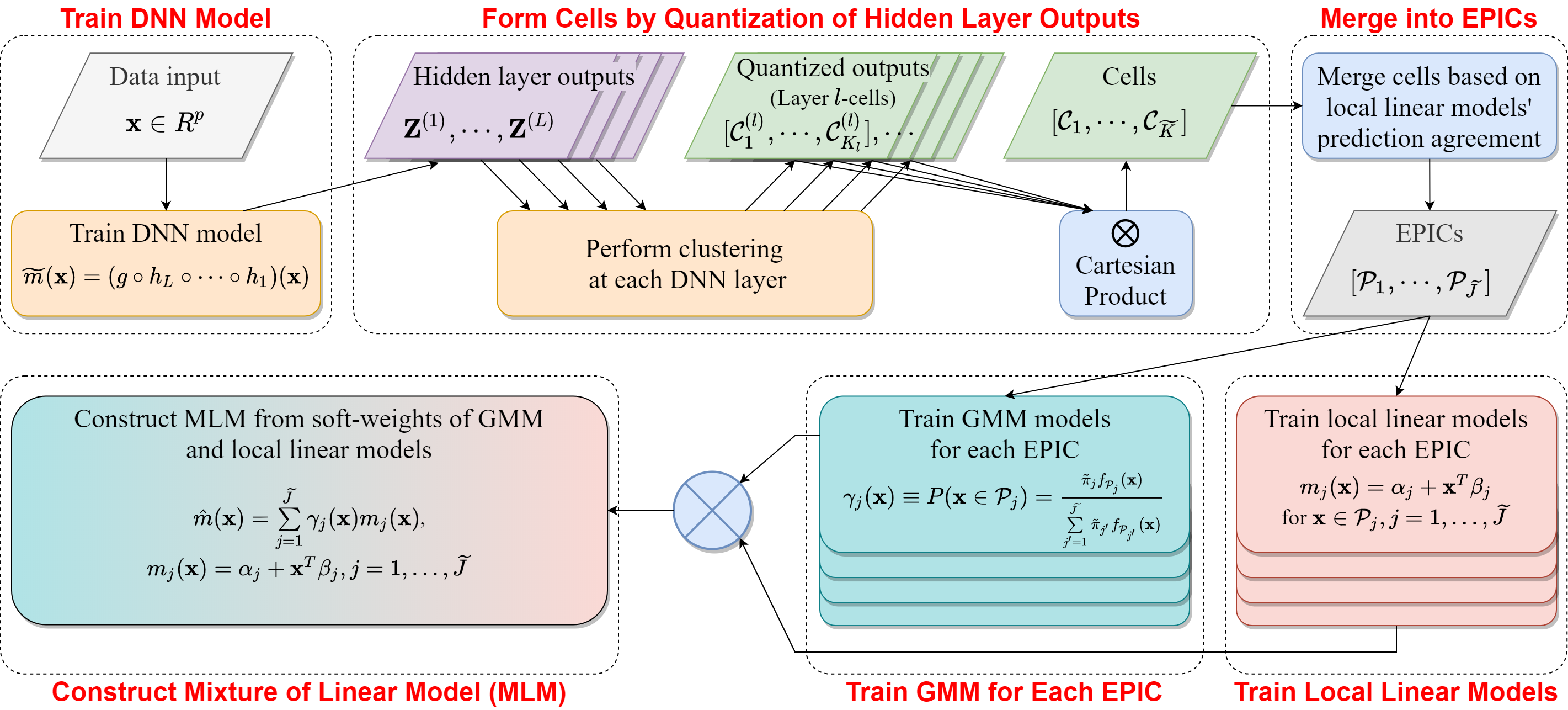
Our core idea is to approximate the prediction function $\widetilde{m}(\mathbf{x})$ of a DNN model by a piecewise linear function $\hat{m}(\mathbf{x})$ called Mixture of Linear Models (MLM). We will present in the context of regression. Adaption to classification will be remarked upon later. Suppose the input sample space $\mathcal{X}$ is divided into $K$ mutually exclusive and collectively exhaustive sets, $\{\mathcal{P}_{1},...,\mathcal{P}_{K}\}$, which form a partition of $\mathcal{X}$. Denote the partition by $\mathscr{P}=\{\mathcal{P}_{1},...,\mathcal{P}_{K}\}$. The partition $\mathscr{P}$ induces a row-wise separation of the input data matrix $\mathbf{X}$ into $K$ sub-matrices: $\mathbf{X}^{(1)}$, …, $\mathbf{X}^{(K)}$. Within each $\mathcal{P}_{k}$, $\widetilde{m}(\mathbf{x})$ is approximated by $m_{k}(\mathbf{x})$, which is referred to as the local linear model. To create $\mathscr{P}$, our criterion is not based on the proximity of $\mathbf{x}_{i}$’s but on the similarity between $\widetilde{m}(\mathbf{x})$ in the neighborhood of each $\mathbf{x}_{i}$. Because of this difference from the conventional mixture model, we are motivated to cluster $\mathbf{x}_{i}$’s by simulating from the prediction function of an estimated DNN. Without the guidance of the DNN, there will not be enough training points in the neighborhood of any $\mathbf{x}_{i}$ to permit a reasonable estimation of the prediction function unless the dimension is very low.

Let $I_{\mathcal{P}}(\mathbf{x})$ be the indicator function that equals $1$ when $\mathbf{x}\in\mathcal{P}$ and zero otherwise. Given the partition $\mathscr{P}$, we express $\hat{m}(\mathbf{x})$ by

$$\hat{m}(\mathbf{x}) = I_{\mathcal{P}_{1}}(\mathbf{x})m_{1}(\mathbf{x})+\cdots+I_{\mathcal{P}_{K}}(\mathbf{x})m_{K}(\mathbf{x}),$$

$$m_{k}(\mathbf{x}) = \alpha_{k}+\mathbf{x}^{T}\mathbf{\beta}_{k},\qquad k=1,...,K.$$ (5)

A schematic plot is provided in Figure 1 to show the major steps in generating an MLM. The partition $\mathscr{P}$ is obtained by a two-stage process. First, clustering is performed based on the outputs at each layer of the DNN. This stage provides refined clusters, referred to as cells, of the data points and helps reduce computation at the next stage. Secondly, the cells are merged into larger clusters based on the similarity of $\widetilde{m}(\mathbf{x})$ computed via simulations. Clusters obtained at this stage become $\mathcal{P}_{k}$’s in $\mathscr{P}$. We refer to $\mathcal{P}_{k}$ as an EPIC (Explainable Prediction-induced Input Cluster). A linear model is then fitted based on the data points in each EPIC as well as simulated data generated using the DNN. GMM models are then formed for each EPIC so that test data can be classified into the EPICs. Finally, a soft-weighted MLM modified from Eq. (5) is used as $\hat{m}(\mathbf{x})$.

The interpretability of MLM relies on both the local linear models $m_{k}(\mathbf{x})$ and the characterization of EPICs. We develop a visualization method and a decision-tree based method to help users explain EPICs and to open avenues for potential discovery. These methods are presented in Section 3.2. Next, we describe the steps to build an MLM.

3.1 Construction of a Mixture of Linear Models

In Subsection 3.1.1, an approach is presented to approximate a neural network by a piecewise linear model and obtain cells. The approach to merge cells and obtain EPICs is described in Subsection 3.1.2. Finally, we describe the soft-weighted form of MLM in Subsection 3.1.3.

3.1.1 Piecewise Linear Approximation of DNN

The neural network model $\widetilde{m}(\mathbf{x})$ in Eq. (4) is non-linear due to the non-linear activation functions $\sigma_{l}(\cdot)$ at each hidden layer. If the outputs at each layer are partitioned such that the non-linearity can be neglected within a cluster, the mapping of DNN from the original input to the prediction is approximately linear for data points that belong to the same cluster across all the layers. Since we will build a linear model for each EPIC, we are motivated to cluster the outputs at each layer of the DNN and use this sequence of clustering results to form the final grouping of the original points. Because clustering is applied to the outputs of the layers, points that belong to the same cluster are not necessarily close in the original space $\mathcal{X}$.

Let $\{\mathcal{C}^{(l)}_{1},\cdots,\mathcal{C}^{(l)}_{K_{l}}\}$ be a partition of the $l$-th layer outputs of the DNN, where $K_{l}$ is the number of clusters. We call this partition layer $l$-cells. Then, with layer $l$-cells, we can approximate the $l$-th hidden layer map $h_{l}(\mathbf{z}^{(l-1)})$ as a piecewise linear function:

$$\hat{h}_{l}(\mathbf{z}^{(l-1)})=I_{\mathcal{C}^{(l)}_{1}}(\mathbf{z}^{(l-1)})(\mathbf{W}^{(1)}_{1}\mathbf{z}^{(l-1)}+\mathbf{b}^{(1)}_{1})+\cdots+I_{\mathcal{C}^{(l)}_{K_{l}}}(\mathbf{z}^{(l-1)})(\mathbf{W}^{(l)}_{K_{l}}\mathbf{z}^{(l-1)}+\mathbf{b}^{(l)}_{K_{l}}),$$ (6)

where $\mathbf{W}^{(l)}_{k}\in\mathbb{R}^{p_{l}\times p_{l-1}}$ and $\mathbf{b}^{(l)}_{k}\in\mathbb{R}^{p_{l}}$ are model parameters, and $I_{\mathcal{C}_{k}^{(l)}}(\mathbf{z}^{(l-1)})$ is the indicator function.

The layer $l$-cells are obtained by clustering the observed $l$-th hidden layer outputs. Denote by $\{\mathbf{z}^{(l)}_{i}\}_{i=1}^{n}$ the observed $l$-th hidden layer outputs corresponding to $\{\mathbf{x}_{i}\}_{i=1}^{n}$ respectively, that is, $\mathbf{x}_{i}\rightarrow\mathbf{z}_{i}^{(l)}$. We apply GMM-based clustering on $\{\mathbf{z}^{(l)}_{i}\}_{i=1}^{n}$ with $K_{l}$ clusters, and obtain the following GMM model. Denote the density function by $f(\cdot)$, and the prior, mean, and covariance matrix of each Gaussian component by $\pi^{(l)}_{k}$, $\mu_{k}^{(l)}$, and $\Sigma_{k}^{(l)}$. Then

$$f(\mathbf{z}^{(l)})=\sum\limits_{k=1}^{K_{l}}\pi^{(l)}_{k}\phi(\mathbf{z}^{(l)}|\mu_{k}^{(l)},\Sigma_{k}^{(l)}).$$ (7)

As usual, the maximum a posteriori (MAP) criterion is applied to cluster $\mathbf{z}^{(l)}_{i}$’s based on the GMM. We apply GMM clustering on each hidden layer separately to compute layer $l$-cells. Denote the set of cluster labels for the layer $l$-cells by $\mathcal{K}_{l}=\{1,\cdots,K_{l}\}$. The set of all possible sequences of the cluster labels across the $L$ layers is the Cartesian product $\widetilde{\mathcal{K}}=\mathcal{K}_{1}\times\cdots\times\mathcal{K}_{L}$. Let the cardinality of $\widetilde{\mathcal{K}}$ be $\widetilde{K}_{0}=\prod\limits_{l=1}^{L}K_{l}$. For each sequence in $\widetilde{\mathcal{K}}$, $(k_{1},...,k_{L})$, $k_{l}\in\mathcal{K}_{l}$, assign it a label $k$, $1\leq k\leq\widetilde{K}_{0}$, according to the lexicographic order. Denote the mapping by $(k_{1},...,k_{L})\rightarrow k$. Then, the original input $\mathbf{x}_{i}$ belongs to cluster $\mathcal{C}_{k}$ if $(k_{1},...,k_{L})\rightarrow k$ and $\mathbf{z}_{i}^{(l)}\in\mathcal{C}_{k_{l}}^{(l)}$ for $l=1,...,L$. It can often occur that no $\mathbf{x}_{i}$ corresponds to a particular sequence in $\widetilde{\mathcal{K}}$. Thus the actual number of clusters formed, denoted by $\widetilde{K}$, is smaller than $\widetilde{K}_{0}$.

We call the clusters $\mathcal{C}_{k}$ cells. After obtaining the cells, we estimate a linear model for each cell. As in Eq.(5), the linear model for the $k$th cell is $m_{k}(\mathbf{x})$. To train each local linear model $m_{k}(\mathbf{x})$, we use both the original data points that belong to a cell $k$ and simulated data points perturbed from the original points with responses generated by the DNN model $\widetilde{m}(\mathbf{x})$. A major reason for adding the simulated sample is that a cell usually does not contain sufficiently many points for estimating $m_{k}(\mathbf{x})$, the very difficulty of high dimensions. By the same rationale, we attempt to mimic the decision of the DNN, which is an empirically strong prediction model trained using the entire data. If the DNN can be well approximated, we expect MLM to perform strongly as well. Estimating a linear model using simulated data generated by the DNN is a data-driven approach to approximate the DNN locally. We thus aptly call this practice co-supervision by DNN.

Let $n_{k}$ be the number of observations in $\{\mathbf{x}_{i}\}_{i=1}^{n}$ that belong to cell $\mathcal{C}_{k}$. We have $\sum\limits_{k=1}^{\widetilde{K}}n_{k}=n$. Without loss of generality, let $\{\mathbf{x}^{\prime}_{k,i}\}_{i=1}^{n_{k}}$ be the set of points that belong to cell $\mathcal{C}_{k}$: $\{\mathbf{x}^{\prime}_{k,i}\}_{i=1}^{n_{k}}=\{\mathbf{x}_{j}|\mathbf{x}_{j}\in\mathcal{C}_{k}\text{ for }j=1,\cdots,n\}$ with an arbitrary ordering of $\mathbf{x}^{\prime}_{k,1},\cdots,\mathbf{x}^{\prime}_{k,{n_{k}}}$, and let $y^{\prime}_{k,i}$ for $i=1,\cdots,n_{k}$ be the corresponding dependent variable of $\mathbf{x}^{\prime}_{k,i}$ for $i=1,\cdots,n_{k}$. We denote by $\bar{\mathbf{x}}^{\prime}_{k}$ the sample mean of $\mathbf{x}^{\prime}_{k,1},\cdots,\mathbf{x}^{\prime}_{k,{n_{k}}}$: $\bar{\mathbf{x}}^{\prime}_{k}=\frac{\sum_{i=1}^{n_{k}}\mathbf{x}^{\prime}_{k,i}}{n_{k}}$. Then we generate $m$ perturbed sample points $\mathbf{v}_{k,1},\cdots,\mathbf{v}_{k,m}$ by adding Gaussian noise to the mean $\bar{\mathbf{x}}^{\prime}_{k}$ with a pre-specified variance parameter $\epsilon$ for each cell $k=1,\cdots,\widetilde{K}$. That is,

$$\mathbf{v}_{k,i}\sim\mathcal{N}(\bar{\mathbf{x}}^{\prime}_{k},\epsilon),\text{ for }i=1,\cdots,n_{k}.$$ (8)

For the perturbed sample points $\{\mathbf{v}_{k,i}\}_{i=1}^{m}$, the predicted dependent variable $\{w_{k,i}\}_{i=1}^{m}$ is computed using the DNN model $\widetilde{m}(\cdot)$:

$$w_{k,i}=\widetilde{m}(\mathbf{v}_{k,i}),\;\;i=1,\cdots,m.$$ (9)

In the case of classification, the prediction of DNN is the probabilities of the classes. We then generate a class label by taking the maximum. We combine the original sample points and the simulated ones,

$$\{(\mathbf{x}^{\prime}_{k,i},y^{\prime}_{k,i})\}_{i=1}^{n_{k}}\bigcup\{(\mathbf{v}_{k,i},w_{k,i})\}_{i=1}^{m}$$

to train $m_{k}(\mathbf{x})$ for $k=1,...,\widetilde{K}$. For each local linear model, if the dimension $p$ of $X$ is large, we can apply a penalized method such as LASSO to select the variables. For the brevity of presentation below, we introduce unified notations for the original data and the simulated data within each cell: $\mathbf{v}^{\prime}_{k,i}=\mathbf{x}^{\prime}_{k,i}$, $i=1,...,n_{k}$, $\mathbf{v}^{\prime}_{k,n_{k}+i}=\mathbf{v}_{k,i}$, $i=1,...,m$, $w^{\prime}_{k,i}=y^{\prime}_{k,i}$, $i=1,...,n_{k}$, $w^{\prime}_{k,n_{k}+i}=w_{k,i}$, $i=1,...,m$.

We need to pre-choose the hyperparameters $K_{l}$, $l=1,\cdots,L$, $m$, and $\epsilon$. In our experiments, we set $m=100$ and $\epsilon\leq 0.1$, the particular value of which is selected to minimize the training accuracy. For simplicity, we set $K_{1}=K_{2}=\cdots K_{L}$ and choose $K_{1}$ using cross-validation.

3.1.2 MLM based on EPICs

The complexity of MLM in Eq. (5) depends primarily on the number of local linear models. If we fit a local linear model for each cell, that is, to treat a cell directly as a EPIC, there can be unnecessarily too many of them. In addition, to facilitate interpretation of the model $\hat{m}(\mathbf{x})$, we must interpret the EPICs. The task tends to be easier if the number of EPICs is low. Therefore, we further merge the cells by hierarchical clustering to generate the EPICs. The similarity between two cells is defined by the similarity of their corresponding local linear models.

For regression analysis, we define mutual prediction disparity, $d_{s,t}$, between the pair of local linear models $m_{s}(\mathbf{x})$ and $m_{t}(\mathbf{x})$, $s,t\in\{1,...,\widetilde{K}\}$ by

$$d_{s,t}=\frac{1}{n_{s}+n_{t}+2m}\left[\sum\limits_{i=1}^{n_{s}+m}\Big{(}m_{s}(\mathbf{v}^{\prime}_{s,i})-m_{t}(\mathbf{v}^{\prime}_{s,i})\Big{)}^{2}+\sum\limits_{i=1}^{n_{t}+m}\Big{(}m_{s}(\mathbf{v}^{\prime}_{t,i})-m_{t}(\mathbf{v}^{\prime}_{t,i})\Big{)}^{2}\right]\,.$$ (10)

We can take $d_{s,t}$ as a distance measure between the two local linear models. It is the average squared difference between the predicted values by the two models.

For classification, we define $d_{s,t}$ using the inverse of F1-score (Rijsbergen,, 1979):

$$d_{s,t}=\frac{fp+fn}{2\cdot tp}$$ (11)

where $$tp=\left|\{\mathbf{v}^{\prime}_{k,i}|m_{s}(\mathbf{v}^{\prime}_{k,i})=1\text{ and }m_{t}(\mathbf{v}^{\prime}_{k,i})=1,\text{ for }i=1,\cdots,n_{k}+m,\,k=s,t\}\right|\,,$$

$$fp=\left|\{\mathbf{v}^{\prime}_{k,i}|m_{s}(\mathbf{v}^{\prime}_{k,i})=1\text{ and }m_{t}(\mathbf{v}^{\prime}_{k,i})=0,\text{ for }i=1,\cdots,n_{k}+m,\,k=s,t\}\right|\,,$$

$$fn=\left|\{\mathbf{v}^{\prime}_{k,i}|m_{s}(\mathbf{v}^{\prime}_{k,i})=0\text{ and }m_{t}(\mathbf{v}^{\prime}_{k,i})=1,\text{ for }i=1,\cdots,n_{k}+m,\,k=s,t\}\right|\,,$$

and $|\cdot|$ denotes the cardinality of a set.

Treating $d_{s,t}$ as a distance between the $s$th and $t$th cells, $s,t\in\{1,\cdots,\widetilde{K}\}$, we apply hierarchical clustering, specifically, Ward’s linkage (Ward Jr,, 1963), to merge the cells $\mathcal{C}_{1},\cdots,\mathcal{C}_{\widetilde{K}}$ into $\widetilde{J}$ clusters. We assume $\widetilde{J}$ is user specified. Let $\mathcal{J}_{j}$ be the set of the indices of cells that are merged into the $j$th cluster, $j=1,...,\widetilde{J}$. For example, if cell $\mathcal{C}_{1}$ and $\mathcal{C}_{2}$ are merged into the first cluster, then $\mathcal{J}_{1}=\{1,2\}$. Clearly $\bigcup\limits_{j=1}^{\widetilde{J}}\mathcal{J}_{j}=\{1,\cdots,\widetilde{K}\}$. We define the merged cells as a EPIC. For $j=1,...,\widetilde{J}$,

$$\mathcal{P}_{j}=\bigcup\limits_{k\in\mathcal{J}_{j}}\mathcal{C}_{k}\,.$$ (12)

The original data and the simulated data contained in $\mathcal{P}_{j}$ form the set $\displaystyle\bigcup_{k\in\mathcal{J}_{j}}\{(\mathbf{v}^{\prime}_{k,i},w^{\prime}_{k,i})\}_{i=1}^{n_{k}+m}$, based on which we refit a local linear model for the EPIC. With a slight abuse of notation, we still denote each local linear model by $m(\mathbf{x})$:

$$\hat{m}(\mathbf{x}) = I_{\mathcal{P}_{1}}(\mathbf{x})m_{1}(\mathbf{x})+\cdots+I_{\mathcal{P}_{\widetilde{J}}}(\mathbf{x})m_{\widetilde{J}}(\mathbf{x}),$$

$$m_{j}(\mathbf{x}) = \alpha_{j}+\mathbf{x}^{T}\mathbf{\beta}_{j},\text{ for }j=1,...,\widetilde{J}\,.$$ (13)

3.1.3 Soft-weighted MLM based on EPICs

Although Eq. (13) is used to fit the training data, it is not directly applicable to new test data because which $\mathcal{P}_{j}$ a test point belongs to is unknown. We essentially need a classifier for the EPICs: $\mathcal{P}_{1}$, …, $\mathcal{P}_{\widetilde{J}}$. Given how the EPICs are generated in training, one seemingly obvious choice is to compute the DNN inner layer outputs for the test data and associate these outputs to the trained cells and subsequently EPICs. However, this approach hinders us from interpreting the overall MLM because categorization into the EPICs requires complicated mappings of a DNN model, even though the local linear models in MLM are relatively easy to interpret. We thus opt for an easy to interpret classifier for EPICs. We will build a classifier for EPICs using the original independent variables instead of DNN inner-layer outputs. In Subsection 3.2, we will also develop ways for visualization and rule-based descriptions of EPICs.

From now on, we treat the partition of the training data $\mathbf{x}_{i}$, $i=1,...,n$, into the EPICs $\mathcal{P}_{1}$, …, $\mathcal{P}_{\widetilde{J}}$ as the “ground truth” labels when discussing classification of EPICs based on the original variables. Denote the labels by $\zeta_{i}$. We have $\mathbf{x}_{i}\in\mathcal{P}_{\zeta_{i}}$. We first construct a GMM directly from the cells $\mathcal{C}_{1}$, …, $\mathcal{C}_{\widetilde{K}}$ by fitting a single Gaussian density for each cell. Denote the estimated prior, mean, and covariance matrix of $\mathcal{C}_{k}$ by $\hat{\pi}_{k}$, $\hat{\mu}_{k}$, and $\hat{\Sigma}_{k}$, $k=1,...,\widetilde{K}$. The estimated prior $\hat{\pi}_{k}$ is simply the empirical frequency, and $\hat{\mu}_{k}$ is given by the sample mean. The covariance $\hat{\Sigma}_{k}$ can be estimated with different types of structural constraints, e.g., diagonal, spherical, or pooled covariance across components. Recall that $\mathcal{P}_{j}$ contains cells $\mathcal{C}_{k}$ with $k\in\mathcal{J}_{j}$. Let $\phi(\cdot)$ be the Gaussian density. Let the estimated prior of $\mathcal{P}_{j}$ be $\tilde{\pi}_{j}=\sum_{k\in\mathcal{J}_{j}}\hat{\pi}_{k}$. The density of $X$ given that $X\in\mathcal{P}_{j}$ is

$$f_{\mathcal{P}_{j}}(\mathbf{x})=\sum_{k\in\mathcal{J}_{j}}\frac{\hat{\pi}_{k}}{\tilde{\pi}_{j}}\cdot\phi(\mathbf{x}\mid\mu_{k},\Sigma_{k})\,,\quad j=1,...,\widetilde{J}.$$ (14)

The posterior $P(X\in\mathcal{P}_{j}\mid X=\mathbf{x})\propto\tilde{\pi}_{j}f_{\mathcal{P}_{j}}(\mathbf{x})$ is used as the weight for the local linear models in MLM. Let the posterior for $\mathcal{P}_{j}$ be $\displaystyle\gamma_{j}(\mathbf{x})=\frac{\tilde{\pi}_{j}f_{\mathcal{P}_{j}}(\mathbf{x})}{\sum_{j^{\prime}=1}^{\widetilde{J}}\tilde{\pi}_{j^{\prime}}f_{\mathcal{P}_{j^{\prime}}}(\mathbf{x})}$. Then the soft-weighted MLM is

$$\hat{m}(\mathbf{x}) = \sum_{j=1}^{\widetilde{J}}\gamma_{j}(\mathbf{x})m_{j}(\mathbf{x})$$

$$m_{j}(\mathbf{x}) = \alpha_{j}+\mathbf{x}^{T}\mathbf{\beta}_{j},\quad j=1,...,\widetilde{J}.$$ (15)

The above soft-weighted MLM yields more smooth transition between the EPICs. As having been explained in Subsection 3.1.2, the local linear models $m_{j}(\mathbf{x})$ are fitted by least square regression using the original and simulated data in $\mathcal{P}_{j}$. We note that the weights $\gamma_{j}(\mathbf{x})$ play a similar role as the kernel functions in Eq.(2). Instead of using Gaussian density functions centered at each data point, we use $f_{\mathcal{P}_{j}}(\mathbf{x})$, the densities of the EPICs. Another important difference is that we use local linear models trained under the co-supervision of a DNN.

3.2 Interpretation

To interpret MLM, we assume that the local linear model within each EPIC can be interpreted, or useful insight can be gained for each EPIC based on its local linear model. Although this assumption may not always hold depending on the dataset, our focus here is to interpret the EPICs. If we can understand the EPICs, we can better understand the heterogeneity across the sample space in terms of the relationship between the dependent and independent variables. For example, if hypothesis testing is conducted, MLM may indicate that a hypothesis is only meaningful for a sub-population but not the entire population. Our experiments show that the heterogeneity across EPICs can be large, and MLM can achieve considerably higher accuracy than a single linear model.

To help understand EPICs, we develop two approaches, one based on visualization and the other based on descriptive rules. For the first approach, we aim at selecting a small number of variables based on which a EPIC can be well separated from the others. If such a small subset of variables exist, we can visualize the EPIC in low dimensions. The second approach aims at identifying easy-to-describe regions in the sample space that are dominated by one EPIC. We call the first approach the Low Dimensional Subspace (LDS) method and the second the Prominent Region (PR) method.

3.2.1 Interpretation of EPIC by LDS

Recall that we model the density of $X$ in each EPIC, denoted by $f_{\mathcal{P}_{j}}(\mathbf{x})$, $j=1,...,\widetilde{J}$, by a GMM in Eq.(14). The marginal density of $f_{\mathcal{P}_{j}}(\mathbf{x})$ on any subset of variables of $X$ can be readily obtained because the marginal density of any Gaussian component in the mixture is Gaussian. Denote a subset of variable indices by $\mathbf{s}$, $\mathbf{s}\subseteq\{1,...,p\}$. Denote the subvector of $X$ specified by $\mathbf{s}$ by $X_{[\mathbf{s}]}$ and correspondingly the subvector of a realization $\mathbf{x}$ by $\mathbf{x}_{[\mathbf{s}]}$. Denote the marginal density of $X_{[\mathbf{s}]}$ by $f_{\mathcal{P}_{j},\mathbf{s}}(\mathbf{x}_{[\mathbf{s}]})$. Consider EPIC $\mathcal{P}_{j}$ and a particular subset of variables specified by $\mathbf{s}$. Using the marginal densities $f_{\mathcal{P}_{j^{\prime}},\mathbf{s}}(\mathbf{x}_{[\mathbf{s}]})$, $j^{\prime}=1,...,\widetilde{J}$, and applying MAP, we can classify whether a sample point $\mathbf{x}_{i}$, $i=1,...,n$, belongs to $\mathcal{P}_{j}$. Let $\hat{\mathbf{q}}_{j}=(\hat{q}_{j,1},...,\hat{q}_{j,n})$ be the indicator vector for $\mathbf{x}_{i}$ being classified to $\mathcal{P}_{j}$ based on the marginal densities of $X_{[\mathbf{s}]}$:

$$\hat{q}_{j,1}=\left\{\begin{array}[]{ll}1&\tilde{\pi}_{j}f_{\mathcal{P}_{j},\mathbf{s}}(\mathbf{x}_{[\mathbf{s}]})\geq\sum_{j^{\prime}:j^{\prime}\neq j}\tilde{\pi}_{j^{\prime}}f_{\mathcal{P}_{j^{\prime}},\mathbf{s}}(\mathbf{x}_{[\mathbf{s}]})\\ 0&\mbox{otherwise}\,.\end{array}\right.$$

Let $\mathbf{q}_{j}=(q_{j,1},...,q_{j,n})$ be the indicator for EPIC $\mathcal{P}_{j}$ based on the EPIC labels $\zeta_{i}$, that is, $q_{j,i}=1$ if $\zeta_{i}=j$, zero otherwise.

Algorithm to find explainable dimensions $\mathbf{s}_{j}^{*}$ for EPIC $\mathcal{P}_{j}$
1	Set hyper-parameter $0<\xi<1$
2	$\mathbf{s}_{j}^{\dagger}=\emptyset$; $r_{j}^{\dagger}=0$
3	Do while $r_{j}^{\dagger}\leq\xi$ and $|\mathbf{s}_{j}^{\dagger}|<p$
4		Form a collection of sets $\mathcal{S}=\{\mathbf{s}|\mathbf{s}=\mathbf{s}_{j}^{\dagger}\bigcup s\text{ for any }s\in\{1,\cdots,p\}\setminus\mathbf{s}_{j}^{\dagger}\}$
5		Compute $r_{\mathbf{s}}=F_{1}(\hat{\mathbf{q}}_{j},\mathbf{q}_{j})$ for all $\mathbf{s}\in\mathcal{S}$
6		Update $\mathbf{s}_{j}^{\dagger}$: $\arg\max\limits_{\mathbf{s}\in\mathcal{S}}r_{\mathbf{s}}\rightarrow\mathbf{s}_{j}^{\dagger}$
7		Update $r^{\dagger}_{j}$: $r_{\mathbf{s}_{j}^{\dagger}}\rightarrow r^{\dagger}_{j}$
8	Return $\mathbf{s}_{j}^{\dagger}$ and $r^{\dagger}_{j}$ as $(\mathbf{s}_{j}^{*},r_{\mathbf{s}^{*}_{j}})$ if $r^{\dagger}_{j}>\xi$. Otherwise, declare failure to find a valid $\mathbf{s}_{j}^{*}$.

Table 1: The algorithm to find explainable dimensions and the corresponding explainable rate for each EPIC.

We seek for a subset $\mathbf{s}^{*}_{j}$ such that the cardinality $|\mathbf{s}^{*}_{j}|$ is small and $\hat{\mathbf{q}}_{j}$ is close to $\mathbf{q}_{j}$, the disparity between them measured by the F1-score between binary classification results. Denote the F1-score by $F_{1}(\hat{\mathbf{q}}_{j},\mathbf{q}_{j})$, which is larger for better agreement between the binary vectors. In the algorithm presented in Table 1, we find $\mathbf{s}^{*}_{j}$ by step-wise greedy search. In a nutshell, the algorithm adds variables one by one to a set until $F_{1}(\hat{\mathbf{q}}_{j},\mathbf{q}_{j})>\xi$, where $0<\xi<1$ is a pre-chosen hyper-parameter. It is possible that the search does not yield any valid $\mathbf{s}^{*}_{j}$, which indicates that the EPICs cannot be accurately classified and thus easily interpreted. We call variables in $\mathbf{s}^{*}_{j}$ explainable dimensions for EPIC $\mathcal{P}_{j}$ and the F1-score obtained by $\mathbf{s}^{*}_{j}$ explainable rate, which is denoted by $r_{\mathbf{s}^{*}_{j}}$.

3.2.2 Interpretation of EPIC by PR

In this subsection, we explore a more explicit way to characterize EPICs. Using a decision tree, we seek prominent regions that can be defined by a few conditions on individual variables and are in the meanwhile dominated by points from a single EPIC. Such descriptions of EPICs are more direct interpretation than visualization in low dimensions. However, the drawback is that prominent regions are not guaranteed to exist. Given a prominent region, researchers can pose a hypothesis specific to this region rather than for the whole population.

Let $\mathcal{D}$ be a decision tree trained for binary classification by CART (Breiman et al.,, 1984). Let the training class labels be $\mathbf{q}=\{q_{i}|q_{i}\in\{0,1\},\;i=1,\cdots,n\}$ and input data matrix $\mathbf{X}\in\mathbb{R}^{n\times p}$. CART recursively divides the data by thresholding one variable at each split. A leaf node, also called terminal node, is a node that is not split; a pure node is a node that contains sample points from a single class; and a fully grown tree is a tree whose leaf nodes either are pure nodes or contain a single point or multiple identical points. It is assumed that when a node becomes pure, it is not further split. Consider a node denoted by $\mathscr{e}$. Define the depth of $\mathscr{e}$, $d(\mathscr{e})$, as the number of splits to traverse from the root node to $\mathscr{e}$. Define the size of $\mathscr{e}$, $s(\mathscr{e})$, as the number of sample points contained in the node. Define the sample index set $u(\mathscr{e})$ as the set of indices of sample points contained in $\mathscr{e}$, and the decision path of $\mathscr{e}$, denoted by $\mathcal{H}$, as the sequence of split conditions to traverse from the root node to $\mathscr{e}$. $\mathcal{H}$ consists of $d(\mathscr{e})$ number of conditions each expressed by thresholding one variable, e.g., $x_{\cdot,j}>a$ or $x_{\cdot,j}\leq a$.

Again let $\mathbf{q}_{j}=(q_{j,1},\cdots,q_{j,n})$ be the indicator vector for any sample point belonging to EPIC $\mathcal{P}_{j}$. We fit a fully grown decision tree $\mathcal{D}_{j}$ based on $\mathbf{X}$ and the class labels $\mathbf{q}_{j}$ (class 1 means belonging to $\mathcal{P}_{j}$). Let $\psi$ be a pre-chosen threshold, $0<\psi\leq 1$. We prune off the descendant nodes of $\mathscr{e}$ if its proportion of points in class 1 reaches $\psi$:

$$\frac{\sum\limits_{i=1}^{n}I_{u(\mathscr{e})}(i)q_{j,i}}{s(\mathscr{e})}\geq\psi\,.$$ (16)

We collect all the leaf nodes satisfying Eq.(16) with sizes above a pre-chosen minimum size threshold $\eta$. Since leaf nodes are not further split, they are ensured to contain non-overlapping points. Suppose there are $\kappa_{j}$ leaf nodes $\hat{\mathscr{e}}_{\tau}$, $\tau=1,...,\kappa_{j}$, such that $s(\hat{\mathscr{e}}_{\tau})>\eta$ and $\hat{\mathscr{e}}_{\tau}$ satisfies Eq.(16). Denote the decision path of $\hat{\mathscr{e}}_{\tau}$ by $\mathcal{H}_{\tau}$, which contains $d(\hat{\mathscr{e}}_{\tau})$ conditions. In $\mathcal{H}_{\tau}$, one variable may be subject to multiple conditions (that is, this variable is chosen multiple times to split the data). We will identify the intersection region of multiple conditions applied to the same variable, which is in general a finite union of intervals. At the end, a decision path $\mathcal{H}_{\tau}$ specifies a region of the sample space $\mathcal{X}$ by the Cartesian product $\mathcal{R}_{1}\times\mathcal{R}_{2}\times\cdots\times\mathcal{R}_{p}$. If $\mathcal{R}_{j^{\prime}}=\mathbb{R}$, then variable $X_{j^{\prime}}$ does not appear in any condition of $\mathcal{H}_{\tau}$. Suppose $\mathcal{R}_{j^{\prime}_{1}}$, …, $\mathcal{R}_{j^{\prime}_{p^{\prime}}}$ are proper subsets of $\mathbb{R}$. The region given by $\mathcal{H}_{\tau}$ can be described by $\{X_{j^{\prime}_{1}}\in\mathcal{R}_{j^{\prime}_{1}}\}\cap\{X_{j^{\prime}_{2}}\in\mathcal{R}_{j^{\prime}_{2}}\}\cap\cdots\cap\{X_{j^{\prime}_{p^{\prime}}}\in\mathcal{R}_{j^{\prime}_{p^{\prime}}}\}$. We call this form of the region decided by $\mathcal{H}_{\tau}$ an explainable condition.

When the depth of $\mathcal{H}_{\tau}$ is small, the number of conditions $p^{\prime}$ in $\mathcal{H}_{\tau}$ will be small, and thus the explainable condition is simpler. For the sake of interpretation, simpler explainable conditions are preferred. It is also desirable to have large $s(\hat{\mathscr{e}}_{\tau})$, which means that many data points from $\mathcal{P}_{j}$ are covered by this explainable condition. Whether we can find simple explainable conditions that also have high coverage of points depends strongly on the data being analyzed. Hence, the search for explainable conditions can only be viewed as a tool to assist interpretation, but it cannot guarantee that simple interpretations will be generated. In practice, it may suffice to require that class 1 accounts for a sufficiently high percentage of points in $\hat{\mathscr{e}}_{\tau}$ by setting the purity parameter $\psi<1$. With this relaxation, we can find $\hat{\mathscr{e}}_{\tau}$’s with smaller depth.

4 Experiments

In this section, we present experimental results of the proposed methods. We demonstrate prediction accuracy of MLM based on cells (MLM-cell) and EPICs (MLM-EPIC), and interpret the formed EPICs by LDS and PR methods. We use five real-world datasets: two TCGA datasets (Section 4.1), one Parkinson’s disease (PD) clinical dataset (Section 4.4) for classification, the bike sharing demand data (Section 4.2), and California housing price data (Section 4.3) for regression task.

We compare the prediction accuracy of MLM-cell and MLM-EPIC with the following methods: random forest (RF) (Breiman,, 2001), support vector machine (SVR) (Cortes and Vapnik,, 1995), multilayer perceptron (MLP), linear regression (LR), generalized additive model (GAM) (Hastie and Tibshirani,, 1990), Spatial Autoregressive (SAR) (Rey and Anselin,, 2007) (for California housing price data that include spatial variables), multivariate adaptive regression splines (MARS) (only for regression tasks, i.e., bike sharing and California housing datasets) (Friedman,, 1991). To fit these models, the following python packages are utilized: pygam for GAM, pyearth for MARS, pysal for SAR, and scikit-learn for the other methods.

Data						KIRC	SKCM	PD	Bike Sharing	Cal Housing
Number of samples	430	388	756	17379	20640
Number of original features	24	30	753	12	8
Continuous / Ordinal	20	25	753	10	8
Nominal	4	5	0	2	0
After dummy encoding	45	73	753	16	8

Table 2: Data descriptions.

The summary descriptions of each dataset are as follows.

• KIRC and SKCM are the Cancer Genome Atlas Kidney Renal Clear Cell Carcinoma (TCGA-KIRC) (Akin et al.,, 2016) and The Cancer Genome Atlas Skin Cutaneous Melanoma (TCGA-SKCM) clinical datasets, respectively. Both are part of a large collection that is made to study the connection between cancer phenotypes and genotypes. The original datasets include tissue images, clinical data, biomedical data, and genomics data. We only use clinical data in this experiment. For both datasets, the target variable is overall survival (OS) status which is coded in binary, $1$ indicating living and $0$ deceased. The covariates consist of demographic and clinical variables ($24$ for KIRC and $30$ for SKCM) such as age, gender, race, tumor status, dimension of specimen, and so on. After dummy encoding of categorical variables, KIRC has $45$ features and SKCM has $73$ features. Both datasets are available in R package TCGAretriever.

• Bike Sharing (Fanaee-T and Gama,, 2014) is an hourly time series data for bike rentals in the Capital Bikeshare system between years $2011$ and $2012$. The count of total rental bikes is the target variable, and $12$ covariates consist of Year$\,\in\{2011,2012\}$, Month$\,\in\{1,\cdots,12\}$, Hour$\,\in\{0,\cdots,23\}$, Holiday$\,\in\{0,1\}$, Weekday$\,\in\{0,\cdots,6\}$, Working day$\,\in\{0,1\}$, Temperature$\,\in(0,1)$ that is normalized from the original range of $(-8,39)$, Feeling temperature$\,\in(0,1)$ that is normalized from $(-16,50)$, Humidity$\,\in(0,1)$, Wind speed$\,\in(0,1)$, Season$\,\in\{0$(winter), $1$(spring), $2$(summer), $3$(fall)$\}$, Weather$\,\in\{0$(clear), $1$(cloudy), $2$(light rain or snow), $3$(heavy rain or snow)$\}$. After dummy encoding of Season and Weather, we get $16$ covariates.

• Cal Housing (Pace and Barry,, 1997) is a dataset for the median house values in California districts, which are published by the $1990$ U.S. Census. In this dataset, a geographical block group is an instance/unit. The original covariates consist of $8$ features including latitude and longitude which are spatial variables, median income, median house age (house age), average number of rooms, average number of bedrooms (bedrooms), block population (population), average house occupancy (occupancy), and latitude and longitude. Given the average number of rooms and the average number of bedrooms, we compute the average number of non-bedroom rooms as a new covariate to replace the former.

• Parkinson’s Disease (PD) dataset (Sakar et al.,, 2019) is collected from 188 patients with PD and 64 healthy individuals to study PD detection from the vocal impairments in sustained vowel phonations of patients. The target variable is binary with 1 being PD patients and 0 otherwise. The covariates consist of various clinical information generated by processing the sustained phonation of the vowel ’a’ from each subject. Consequently, 753 features are generated by various speech signal processing algorithms, e.g., Time Frequency Features, Mel Frequency Cepstral Coefficients (MFCCs).

For all the datasets, we use dummy encoding for nominal variables. That is, we generate $c-1$ binary vectors for a nominal variable with $c$-classes. The numbers of samples and features used in the experiments are shown in Table 2.

Data					KIRC		SKCM		PD		Bike Sharing	Cal Housing
		(AUC)		(AUC)		(AUC)		(RMSE)		(RMSE)
Model		Train	Test	Train	Test	Train	Test	Train	Test	Train	Test
	Kmeans-mean	.834	.723	.774	.650	.794	.750	122.1	127.7	.795	.815
	RF	.983	.869	.997	.688	.997	.794	43.8	52.2	.421	.554
	SVR	.843	.856	.764	.667	.756	.728	145.6	148.1	.671	.676
	MARS	-	-	-	-	-	-	141.1	140.1	.629	.640
	MLP	.974	.907	.987	.777	.975	.833	40.1	47.6	.503	.517
	LR	.853	.888	.826	.702	.880	.789	141.1	140.3	.723	.727
	SAR	-	-	-	-	-	-	-	-	.655	.652
	GA1M	.838	.847	-	-	-	-	99.4	101.1	.613	.640
	MLM-cell	.904	.891	.948	.728	1.000	.860	52.7	60.9	.560	.570
	MLM-EPIC	.902	.891	.861	.742	.975	.851	62.8	66.7	.569	.584

Table 3: Prediction accuracy of regression and classification methods. We partition these methods into two categories: complex (top panel) and interpretable models (bottom panel). For each method, the model parameters are fine tuned. By linear regression (LR), we specifically mean logistic regression for KIRC, SKCM and PD data, and Poisson regression for Bike Sharing data. If a method is not applicable to a dataset, the corresponding entry in the table is not listed.

4.1 TCGA Clinical Data

For both KIRC and SKCM data, MLP is constructed using $2$ hidden layers that have respectively $128$ and $32$ units for KIRC and $256$ and $32$ units for SKCM, and trained for $10$ epochs. Random forest is trained with maximum depth equal to $10$. For both MLM-cell and MLM-EPIC, hyper-parameters $K_{l}$ is set based on $10$-fold cross validation (CV) within training data, and assumed to be equal across the $2$ hidden layers. We choose another hyper-parameter $\widetilde{J}$ by comparing the training accuracy obtained at several values. For KIRC, the number of layer $l$-cells is set to $K_{l}=4$ according to CV for $l=1,2$, and $12$ cells are formed at the end. These $12$ cells are merged into $\widetilde{J}=10$ EPICs. For SKCM, the number of layer $l$-cells is set to $K_{l}=13$ according to CV for $l=1,2$, and $77$ cells are formed at the end. The cells are merged into $\widetilde{J}=10$ EPICs.

The first two columns of Table 3 show the prediction accuracy for KIRC and SKCM. The area under curve (AUC) score is used here as the efficacy metric. For both datasets, MLP predicts the overall survival (OS) status the best compared to other models. RF has a higher training AUC score but it does not generalize well to the testing data. Among all the interpretable models, GAM does not converge for SKCM. LR for KIRC and SKCM, and GAM for KIRC have higher test AUC scores compared to other complex models although their training AUC scores are not better than RF. On the other hand, MLM-cell and MLM-EPIC achieve relatively high AUC scores in both training and testing accuracy, and outperform LR.

(a) Age

(b) Sex

(c) Radiation treatment adjuvant

(d) History other malignancy

Figure 2: Estimated regression coefficients (blue dots) with their corresponding confidence intervals (purple lines) of four selected variables for SKCM. The X-axis indicates the value of each regression coefficient. The linear effects of age, sex, whether the patient has radiation treatment adjuvant, and whether the patient has the history of other malignancy vary by EPICs.

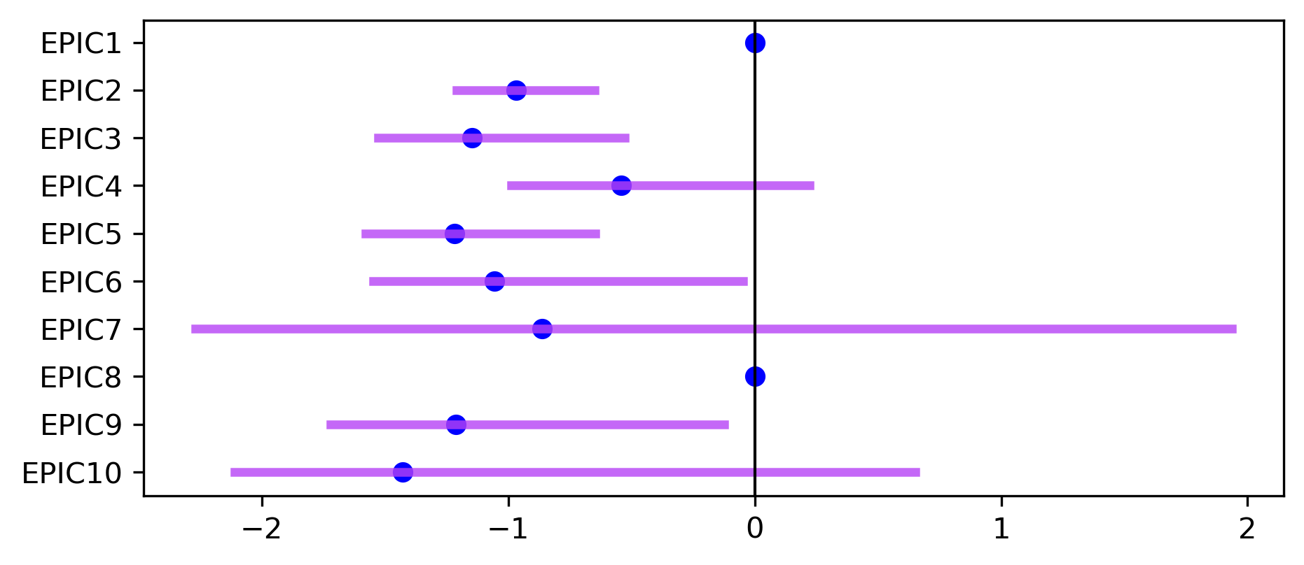
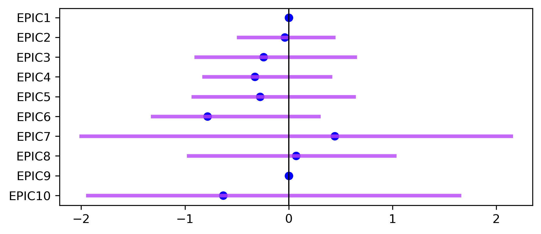
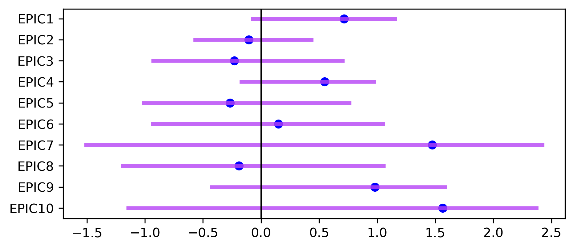
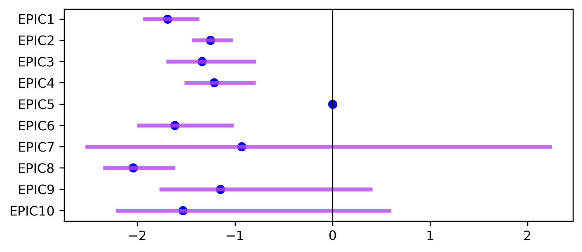
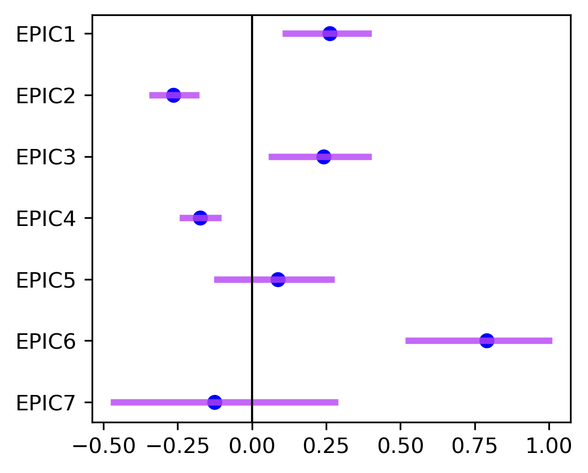
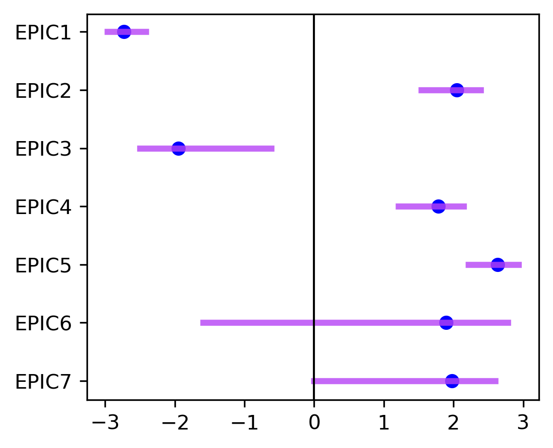
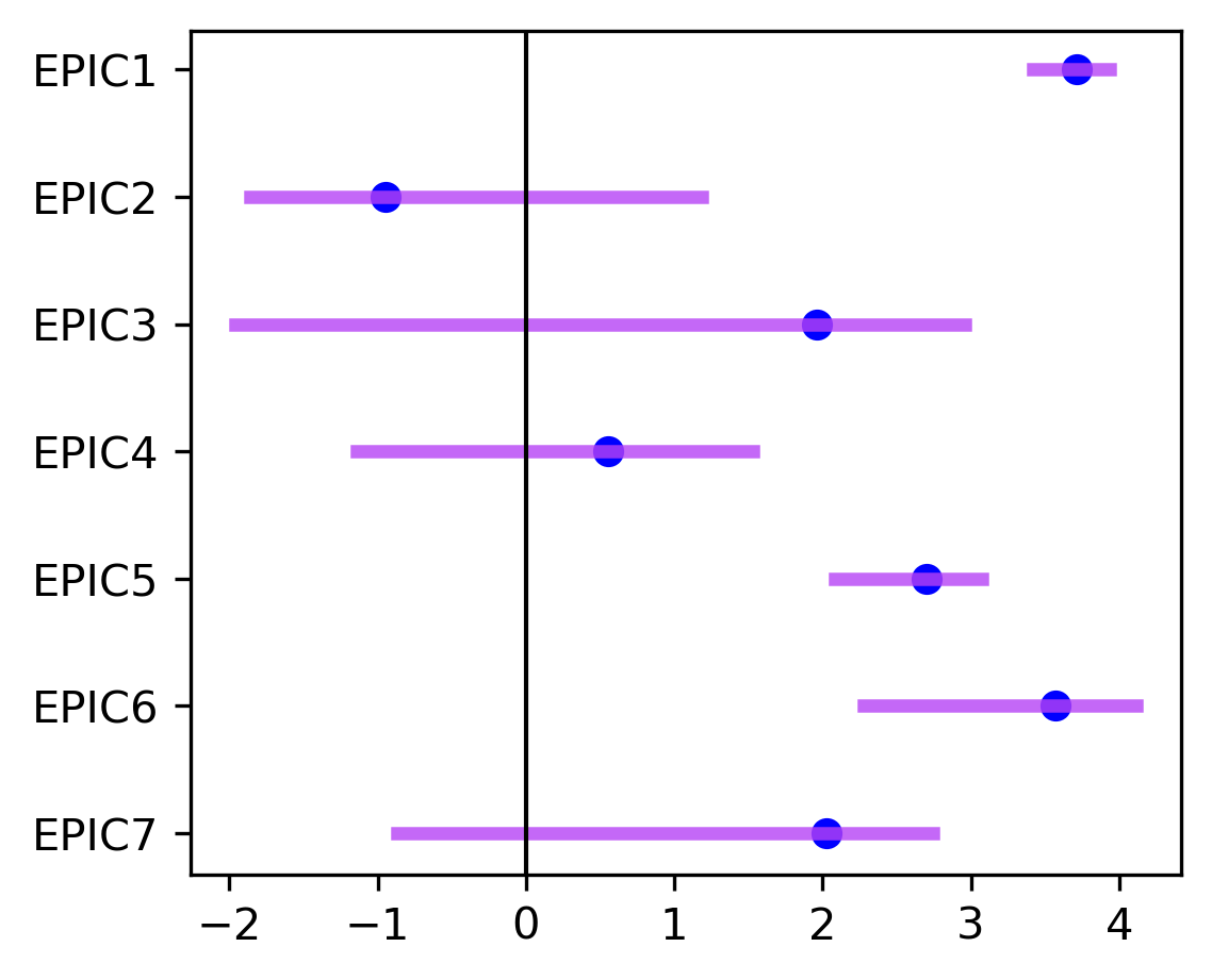
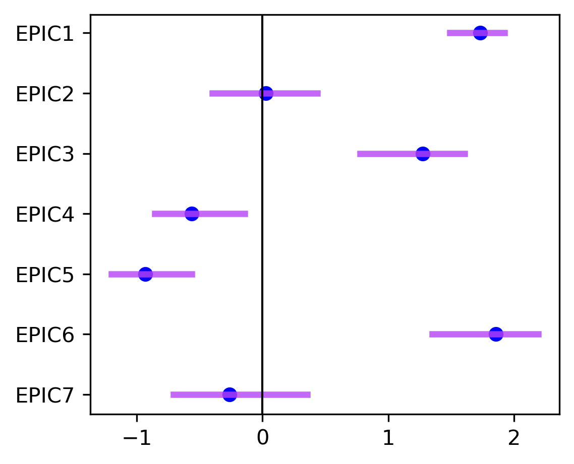
We interpret MLM-EPIC via local linear models for each EPIC. Figure 2 shows the estimated regression coefficients and the associated confidence intervals for four selected variables for SKCM. The EPICs are sorted in descending order according to their sizes. Figure 2(a) demonstrates that age is not significantly associated with the OS status in EPICs 1 and 8, as the coefficients related to age are shrunk to zero by LASSO penalty. However, the irrelevance of age does not hold in other EPICs. Such EPIC-specific results enable us to gain understanding impossible with a single LR model or a DNN.

In addition, EPICs $2$, $3$, $5$, $6$, and $9$ have negative coefficients for age that are significantly different from zero. This result may motivate researchers to examine whether there exists significantly different linear impacts of age between two groups of patients belonging to two different EPICs, e.g., by applying a paired test. Similar analyses can be made to the other three variables. Moreover, Figure 2(d) demonstrates that the prediction model for subjects belonging to EPIC $5$ does not include the history of other malignancy variable, which shows the potential heterogeneous structure among the covariates with respect to OS status.

Now, we investigate how EPICs are formed. We compute explainable conditions for each EPIC to check if they provide any insight into distinguishing EPICs. Here we interpret the largest EPIC that consists $59$ samples. $\psi$ and $\eta$ are set to 1 and 4. Table 4 shows explainable conditions for the EPIC 1. More explainable conditions for other EPICs are provided in Supplementary Material. Specifically, around half of patients in EPIC 1 are relatively young patients who have new tumor events after the initial treatment and have less than 306 survival months. Combining this information with the information from Figure 2, an interesting hypothesis can be that for the patients in EPIC 1 under these conditions, age does not impact the OS status. Such insight is not available from MLP or other complex models which are hard to interpret.

EPIC			Descriptions	Size
1	Age$\,<29.0$, Days to collection$\,\leq 10345$, Initial pathology DX year$\,>1996$, New tumor event after initial treatment$\,=1$, Overall survival months$\,\leq 306.2$, Retrospective collection$\,=1$, AJCC staging edition$\,\neq 5$	11
(59)	Age$\,<29.0$, $8701<\,$Days to collection$\,>10345$, Initial pathology DX year$\,>1996$, New tumor event after initial treatment$\,=1$, Overall survival months$\,\leq 306.2$, Retrospective collection$\,=1$, Submitted tumor DX days$\,>9737$, AJCC staging edition$\,\neq 5$	8
	Age$\,<29.0$, Days to collection$\,>10345$, ICD-10$\,<5$, ICD-O-3 site$\,>23.5$, Overall survival months$\,\leq 306.2$, Retrospective collection$\,=1$, AJCC staging edition$\,\neq 5$	7

Table 4: Explainable conditions for the largest EPIC for SKCM data. Numbers within the bracket indicate the size of the EPIC in training data.

4.2 Bike Sharing Data

The bike sharing dataset is often used to demonstrate the efficacy of complex machine learning models. For this dataset, RF is set with its maximum depth equal to $10$. MLP is constructed with $3$ layers and $30$ units for each layer, and trained for $20$ epochs. MLM-cell is computed based on the MLP as its underlying neural network model. The number of layer $l$-cells is $100$ chosen by CV and it is set equal across the $3$ hidden layers. $1712$ cells are formed. MLM-EPIC is constructed by merging $1712$ cells into $150$ EPICs. For the estimation of the MLM-EPIC parameters, we apply pooled covariance to estimate GMM of each EPIC. Pooled covariance is often used in the model-based clustering when cluster sizes are unbalanced. Pooled covariance mitigates the tendency that samples tend to be assigned to large clusters. For other methods, we apply the default settings of the methods from pyearth (for MARS), pygam (for GAM), and scikit-learn python packages.

First, we examine the prediction accuracy of the methods. Table 3 shows that RF and MLP achieve higher prediction accuracy (lower root mean squared error (RMSE)) in comparison to other simpler methods. The RMSEs of MLM-cell and MLM-EPIC are considerably lower than any other method except for RF and MLP. Figure 3 (a) and (b) show the trade-off between the prediction accuracy and the model complexity of MLM (indicated by $K_{l}$ for MLM-cell in (a) and by $\widetilde{J}$ for MLM-EPIC in (b)). As the model complexity increases, both training and testing RMSE decreases. We do not observe overfitting as the model complexity of MLM is capped by the underlying neural network. The measure for agreement between MLP and MLM-cell is computed by the RMSE between the predicted values of MLP and MLM-cell respectively. As shown in the figure, the agreement with MLP decreases as the model complexity increases. Figure 3 (c) is the histogram of EPIC sizes obtained from the $150$ EPICs of the training data. The histogram shows that many data points belong to small EPICs. For the sample points in small EPICs, the predicted values based on MLM-EPIC are similar to using the nearest neighbor method. For example, in the extreme case, if all EPICs consist of a single point, MLM-EPIC is equivalent to using $1$-nearest neighbor method.

Figure 3: Impact of hyper-parameters, $K_{l}$ and $\widetilde{J}$, on MLM for bike sharing data. (a) RMSE of MLM-cell at different $K_{l}$, the number of layer $l$-cells. (b) RMSE of MLM-EPIC at different $\widetilde{J}$, the number of EPICs. (c) Histogram of the sizes of the $150$ EPICs.

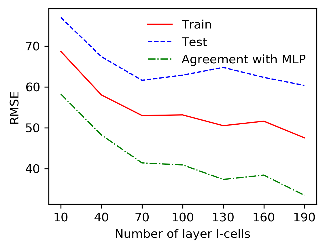
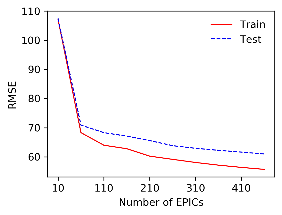
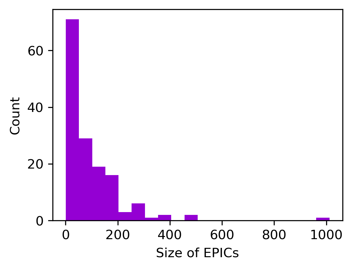
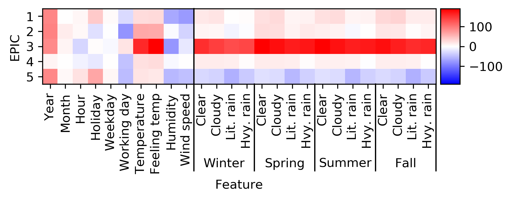
Figure 4 shows the fitted regression coefficients of MLM-EPIC for the 5 largest EPICs. The values of the coefficients are indicated by color. Depending on which EPIC a sample point belongs to, the effect of a covariate is different when predicting the bike rental count. Specific interpretation of the fitted MLM-EPIC is provided in Supplementary Material.

Figure 4: The linear mixture model regression coefficients $\{\mathbf{\hat{\beta}}_{j}|\mathbf{x}\in\mathcal{P}_{j}\}_{j=1}^{\widetilde{J}}$ for the top $5$ largest EPICs for bike sharing data.

4.3 California Housing Prices

California housing data was first introduced to demonstrate the efficacy of spatial autoregressive (SAR) model (Pace and Barry,, 1997), yet the data is now often used to test various neural network models. Many previous works have shown that neural network models perform well with spatial data (Zhu,, 2000; Özesmi and Özesmi,, 1999), however they cannot be interpreted. In this subsection, we analyze California housing price data with MLM for both prediction and interpretation.

Table 3 shows the prediction accuracy of the methods. RF is fitted with its maximum depth equal to $10$, and MLP is constructed with $3$ hidden layers and $30$ hidden units for each layer. MLP is trained for $50$ epochs. SAR is fitted with the consideration of spatially lagged covariates except for longitude and latitude. MLM-cell and MLM-EPICs are fitted based on the MLP model. MLM-cell is constructed with layer $l$-cells equal to $6$ for all $3$ layers, and consequently forms $64$ cells. MLM-EPIC merged the $64$ cells into $30$ EPICs. The prediction accuracy of MLM-cell and MLM-EPIC is slightly lower (i.e., slightly larger RMSE) than that of MLP and RF, but they achieve better accuracy than any other interpretable models such as LR, SAR, and GAM.

(a) Median income

(b) House age

(c) Other rooms

(d) Bedrooms

(e) Population

(f) Occupancy

Figure 5: Log-valued regression coefficients of local linear models plotted on longitude (horizontal axis) and latitude (vertical axis) space. Regression coefficients differ for each EPIC.

(a) Median income

(b) House age

(c) Other rooms

(d) Bedrooms

(e) Population

(f) Occupancy

Figure 6: Log-valued confidence intervals of each variable in the $7$ largest EPICs.

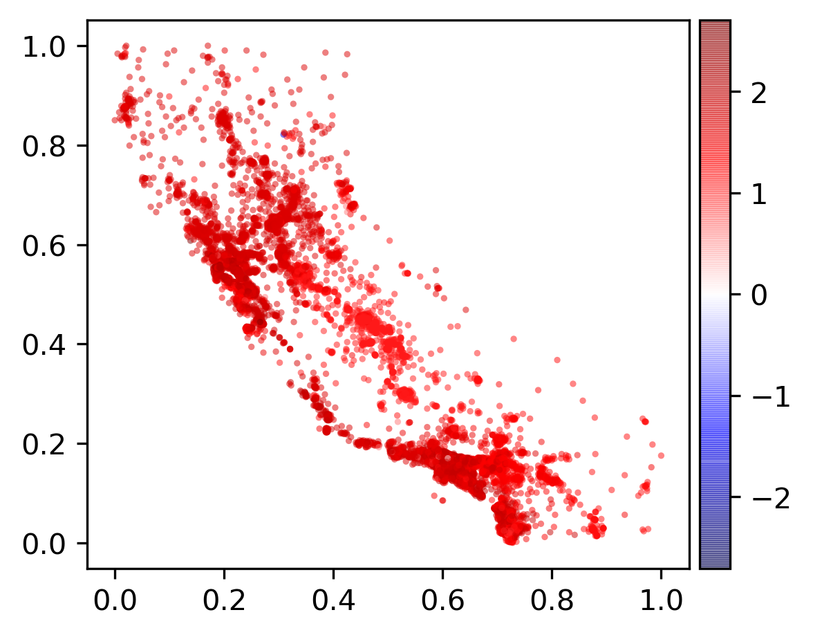
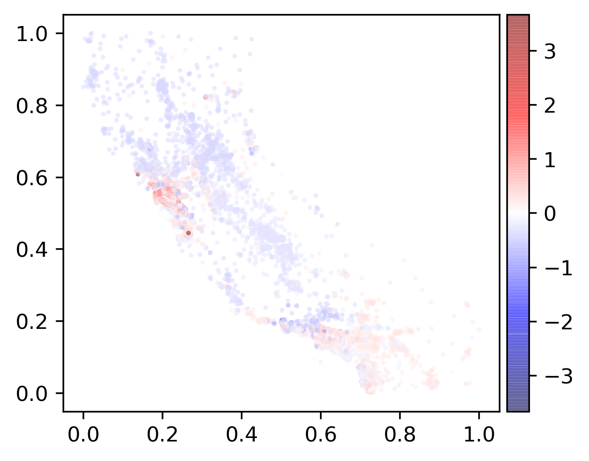
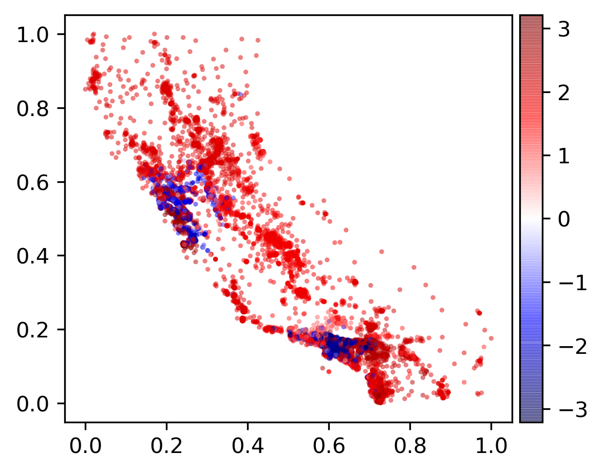
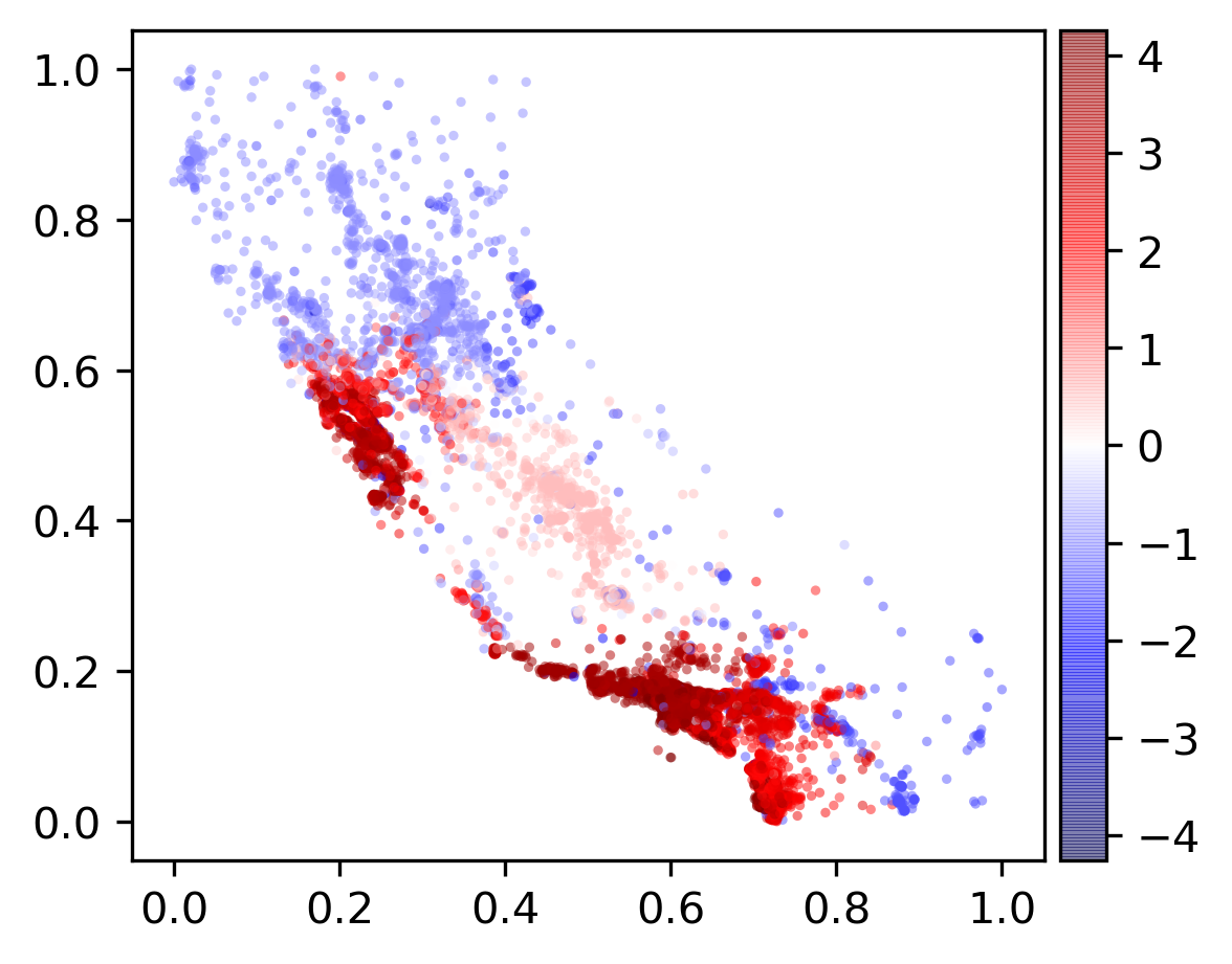
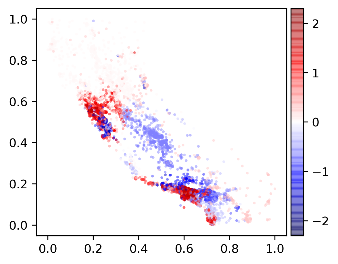
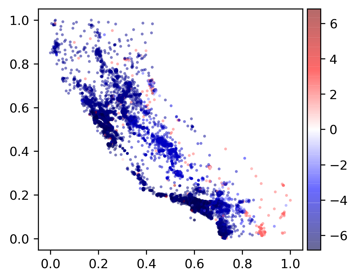
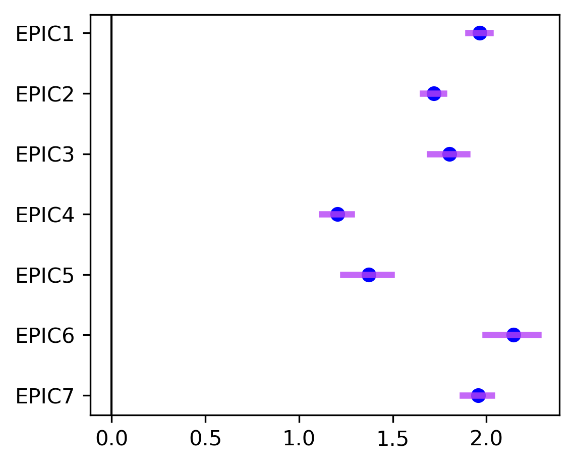
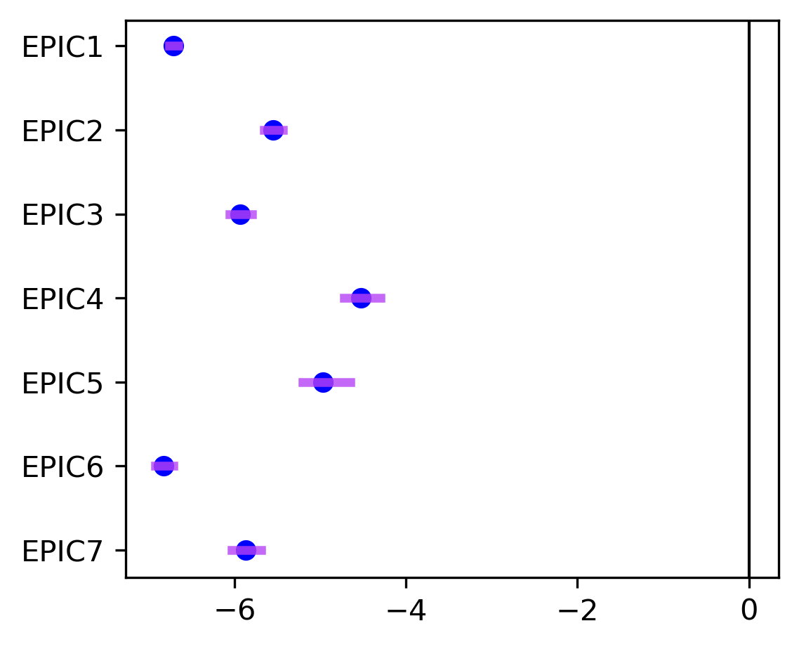
MLM-EPIC provides more useful interpretation than those commonly-used autoregressive models for California housing price data. Autoregressive models are primarily used to describe a time-varying or space-varying process, and the interpretation of the model is based on the model’s representation of time or spatial variables. MLM-EPIC can be utilized to describe both time and space-varying effects as it divides samples into EPICs in different time and space. Figure 5 shows the change of regression coefficients for each variable in the longitude and latitude space. The value of the coefficient for the variable in consideration is indicated by color. According to the fitted MLM-EPIC, the impact of the median income on the house values is relatively consistent across the California map. On the other hand, house age affects the house values differently depending on which EPIC the sample points belong to. Near the coastal area, old houses tend to be appreciated whereas in the inland area, house age has a negative impact on the house value. This observed pattern may be explained by the fact that the houses in the highly populated area were built in earlier days and are still in high demand. Another interesting pattern in Figure 5 is that the increase of the number of non-bedroom rooms has a negative impact on the house values in city center areas. The log-valued confidence intervals and estimates of the $6$ covariates are shown in Figure 6 for the first $7$ biggest EPICs. In training data, the $7$ EPICs cover about $70\%$ of the samples.

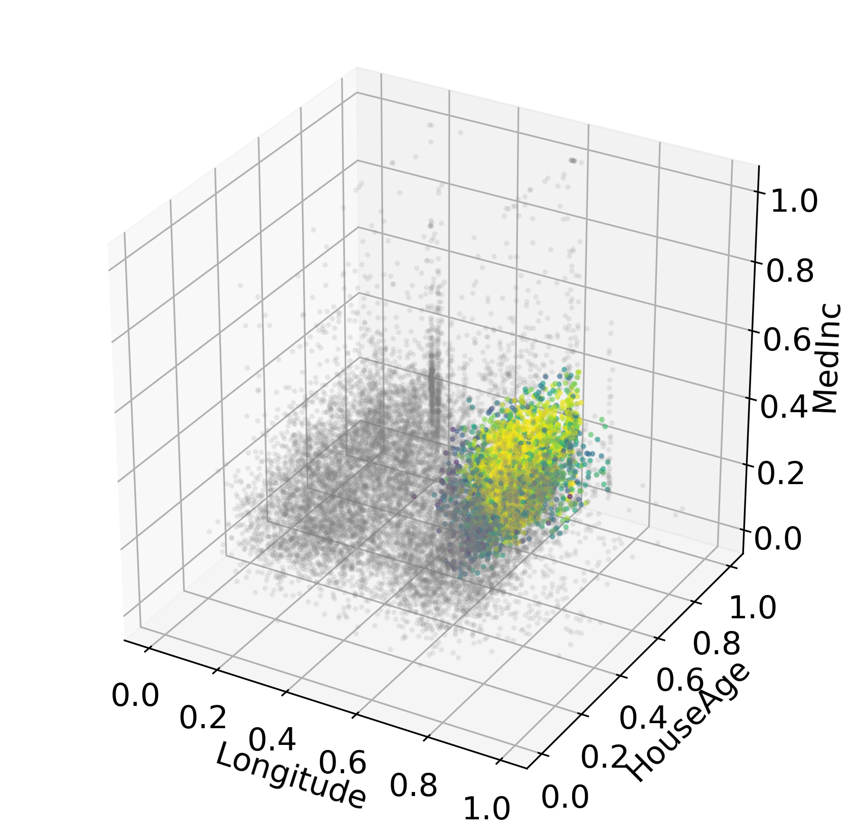
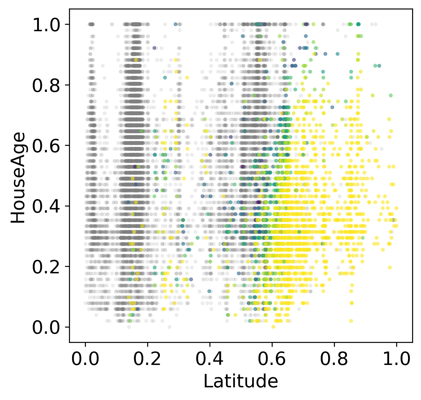
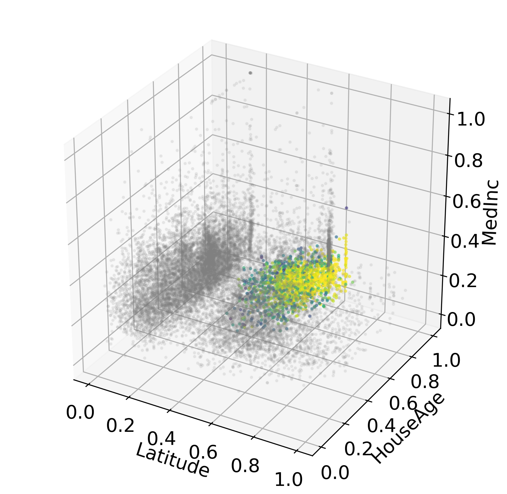
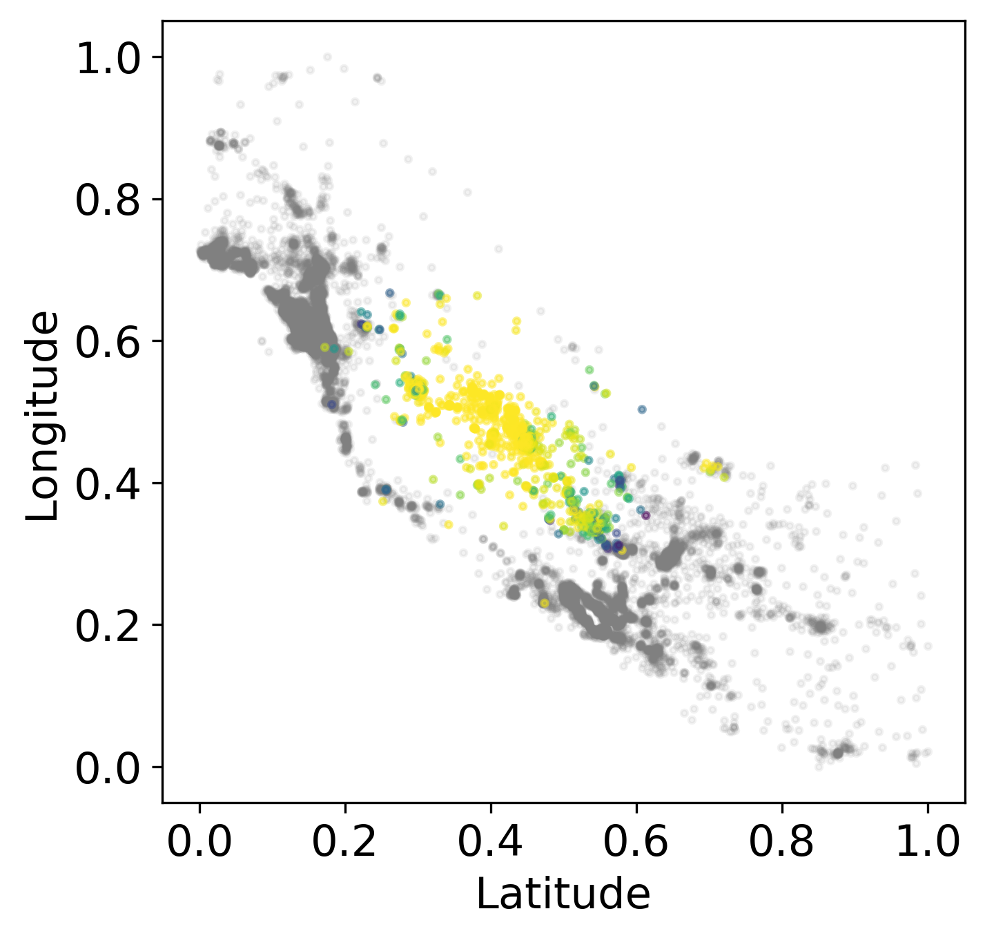
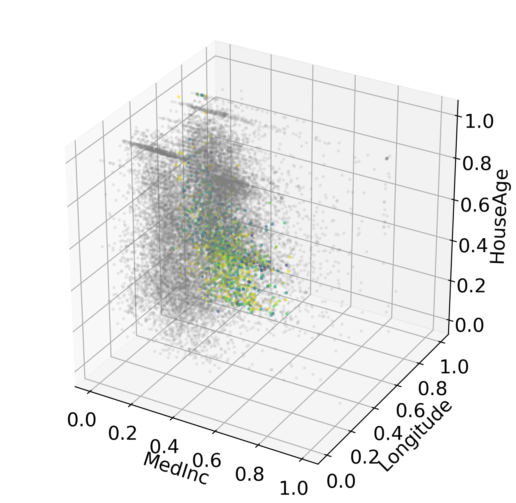
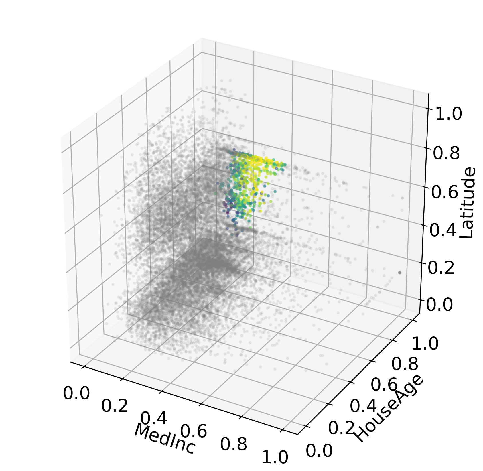
For this dataset, we cannot get concise explainable conditions for the EPICs. For example, an explainable condition for EPIC $1$ is ‘Median income$\,\leq 86.6k$ and House age$\,\notin(3.5,27.5]$ and Bedrooms$\,\notin(33.1,33.6]$ and Population$\,\notin(32.1k,35.7k]$ and Average occupancy$\,\notin(1239.6,1241.8]$ and Latitude$\,\notin(40.1,40.9]$ and Longitude$\,\notin(-121.2,-119.5]$’. Instead, we use the LDS method to find explainable dimensions for the EPICs. The explainable dimensions for the first $6$ biggest EPICs are shown in Figure 7. For example, based on $3$ features: Median income, House age, Longitude, EPIC $1$ is distinguishable from the other EPICs with accuracy $0.84$ as measured by F-1 score. EPIC $1$ mostly contains points with lower than the median income, older than the median house age, and the middle east part of California. In EPIC $1$, older houses tend to increase the house values slightly. Also, having more bedrooms is appreciated in house values, while the increase of rooms other than bedrooms tends to decrease the house values. EPIC $2$ contains mostly points with newer houses in the middle northern part of California (with the explainable rate equal $0.82$). For points in EPIC $2$, in contrast to EPIC $1$, the house age has a negative impact on the house value. Also, the increase in the number of rooms other than bedrooms tends to increase the house value, whereas the impact of the number of bedrooms is not significant.

(a) EPIC 1 (0.84)

(b) EPIC 2 (0.82)

(c) EPIC 3 (0.80)

(d) EPIC 4 (0.88)

(e) EPIC 5 (0.58)

(f) EPIC 6 (0.81)

Figure 7: Explainable dimensions for the first $6$ biggest EPICs. The values in the parentheses are explainable rates of the explainable dimensions for each EPIC.

4.4 Parkinson’s Disease Detection

Many works have studied Parkinson’s disease (PD) to detect PD from the vocal impairments in sustained vowel phonatations of PD patients. However, due to the lack of clear understanding of the mechanism to detect PD from the complex characteristics that appear in the mere voice recordings of PD patients, the dataset often involves a huge number of covariates that are extracted from various speech signal processing algorithms. In this subsection, we demonstrate that MLM-cell and MLM-EPIC work well with this high-dimensional dataset. At reduced complexity, the two methods achieved slightly better accuracy than the more complex models.

For this dataset, RF is fitted with maximum depth equal to $10$. MLP is constructed with $3$ layers that have $30$ hidden units for each layer. MLP is trained for $5$ epochs. Other methods follow the default parameter setting from sci-kit learn python package. MLM-cell is constructed based on MLP with layer-$l$ cells equal to $5$, which is chosen by CV, for $l=1,2,3$. $52$ cells are formed. We merge the cells into $3$ EPICs to build MLM-EPIC. For the local linear models of MLM-EPIC, we applied LASSO penalty with its weight parameter $\alpha=0.2$.

Table 3 shows the training and testing accuracy of the methods. MLM-cell achieves the highest training and testing accuracy. In addition, although MLM-EPIC is only a mixture of $3$ local linear models, it has better testing accuracy (lower testing AUC) than MLP. Specifically, MLM-EPIC forms $3$ EPICs with sizes $442$, $133$, and $29$ for the training data. The local linear models respectively have $700$, $14$, $0$ non-zero regression coefficients. The last local linear model is a constant function which classifies all the points in EPIC 3 as class 0. In this case, the interpretation of EPIC 3 provides an explanation of a local region for class 0.

We compute the explainable dimensions for each EPIC. We set $\xi=0.8$. EPIC 1 is distinguishable with only one variable. In fact, $694$ single variables achieve an explainable rate higher than $0.8$. Among them, the variable ’tqwt_TKEO_std_dec_12’ achieves the highest explainable rate of $0.87$. Whereas, EPIC 2 needs 7 variables to distinguish the EPIC with explainable rate higher than $0.8$, and EPIC 3 needs 13 variables.

Explainable conditions provide a different perspective for interpreting the EPICs. With $\psi=0.9$ and $\eta=50$ for EPIC 1 and 2, and $\eta=5$ for EPIC 3, we find the explainable conditions listed in Table 5. In the explainable conditions, ’tqwt_TKEO_std_dec_12’ appears again as an important feature to distinguish EPIC 1. EPIC 2 and 3 are relatively hard to be distinguished with explainable conditions as the explainable conditions only capture 75 out of 133 points for EPIC 2, and 9 out of 29 points for EPIC 3.

EPIC			Descriptions	Size
1 (442)	std_delta_delta_log_energy$\,>0.057$, tqwt_energy_dec_18$\,\leq 0.562$,	381
	tqwt_TKEO_std_dec_12$\,\leq 0.102$, tqwt_medianValue_dec_31$\,\leq 0.454$
2 (133)	mean_MFCC_2nd_coef$\,\leq 0.397$, tqwt_entropy_log_dec_27$\,\leq 0.696$,	75
	tqwt_entropy_log_dec_35$\,>0.368$, tqwt_TKEO_std_dec_17$\,\leq 0.216$
3 (29)	tqwt_entropy_shannon_dec_8$\,\leq 0.007$, tqwt_stdValue_dec_19$\,>0.373$	9

Table 5: Explainable conditions for the $3$ EPICs for Parkinson’s disease data. Numbers in the bracket indicates the size of EPIC in training data.

5 Conclusions

In this paper, we develop MLM under co-supervision of a trained DNN. Our goal is to estimate interpretable models without compromising performance. The experiments show that MLM achieves higher prediction accuracy than other explainable models. However, for some data sets, the gap between the performance of MLM and DNN is not negligible. Interpretation is intrinsically subjective. For different datasets, different approaches can be more suitable. We have developed a visualization method and a decision rule-based method to help understand the prediction function. In any case, these methods rely heavily on the local linear models constructed in MLM. To explore the aspect of interpretation at greater depth, as future work, we plan to examine applications in more specific context.

References

- Agarwal et al., (2020) Agarwal, R., Frosst, N., Zhang, X., Caruana, R., and Hinton, G. E. (2020). Neural additive models: Interpretable machine learning with neural nets. arXiv preprint arXiv:2004.13912.
- Akin et al., (2016) Akin, O., Elnajjar, P., Heller, M., Jarosz, R., Erickson, B., Kirk, S., and Filippini, J. (2016). Radiology data from the cancer genome atlas kidney renal clear cell carcinoma [tcga-kirc] collection. The Cancer Imaging Archive.
- Bahdanau et al., (2014) Bahdanau, D., Cho, K., and Bengio, Y. (2014). Neural machine translation by jointly learning to align and translate. arXiv preprint arXiv:1409.0473.
- Breiman, (2001) Breiman, L. (2001). Random forests. Machine learning, 45(1):5–32.
- Breiman et al., (1984) Breiman, L., Friedman, J., Stone, C. J., and Olshen, R. A. (1984). Classification and regression trees. CRC press.
- Chen et al., (2019) Chen, C., Li, O., Tao, D., Barnett, A., Rudin, C., and Su, J. K. (2019). This looks like that: deep learning for interpretable image recognition. Advances in neural information processing systems, 32:8930–8941.
- Cleveland and Devlin, (1988) Cleveland, W. S. and Devlin, S. J. (1988). Locally weighted regression: an approach to regression analysis by local fitting. Journal of the American statistical association, 83(403):596–610.
- Cortes and Vapnik, (1995) Cortes, C. and Vapnik, V. (1995). Support-vector networks. Machine learning, 20(3):273–297.
- Doshi-Velez and Kim, (2017) Doshi-Velez, F. and Kim, B. (2017). Towards a rigorous science of interpretable machine learning. arXiv preprint arXiv:1702.08608.
- Fanaee-T and Gama, (2014) Fanaee-T, H. and Gama, J. (2014). Event labeling combining ensemble detectors and background knowledge. Progress in Artificial Intelligence, 2(2):113–127.
- Friedman, (1991) Friedman, J. H. (1991). Multivariate adaptive regression splines. The annals of statistics, pages 1–67.
- Guo et al., (2020) Guo, M., Zhang, Q., Liao, X., and Zeng, D. D. (2020). An interpretable neural network model through piecewise linear approximation. arXiv preprint arXiv:2001.07119.
- Guo et al., (2019) Guo, T., Lin, T., and Antulov-Fantulin, N. (2019). Exploring interpretable lstm neural networks over multi-variable data. arXiv preprint arXiv:1905.12034.
- Guo et al., (2018) Guo, W., Huang, S., Tao, Y., Xing, X., and Lin, L. (2018). Explaining deep learning models – a bayesian non-parametric approach. In Bengio, S., Wallach, H., Larochelle, H., Grauman, K., Cesa-Bianchi, N., and Garnett, R., editors, Advances in Neural Information Processing Systems, volume 31. Curran Associates, Inc.
- Hastie and Tibshirani, (1990) Hastie, T. J. and Tibshirani, R. J. (1990). Generalized additive models, volume 43. CRC press.
- Lou et al., (2013) Lou, Y., Caruana, R., Gehrke, J., and Hooker, G. (2013). Accurate intelligible models with pairwise interactions. In Proceedings of the 19th ACM SIGKDD international conference on Knowledge discovery and data mining, pages 623–631.
- Lundberg and Lee, (2017) Lundberg, S. M. and Lee, S.-I. (2017). A unified approach to interpreting model predictions. In Advances in neural information processing systems, pages 4765–4774.
- Molnar, (2020) Molnar, C. (2020). Interpretable Machine Learning. Lulu. com.
- Nadaraya, (1964) Nadaraya, E. A. (1964). On estimating regression. Theory of Probability & Its Applications, 9(1):141–142.
- Nair and Hinton, (2010) Nair, V. and Hinton, G. E. (2010). Rectified linear units improve restricted boltzmann machines. In Icml.
- Özesmi and Özesmi, (1999) Özesmi, S. L. and Özesmi, U. (1999). An artificial neural network approach to spatial habitat modelling with interspecific interaction. Ecological modelling, 116(1):15–31.
- Pace and Barry, (1997) Pace, R. K. and Barry, R. (1997). Sparse spatial autoregressions. Statistics & Probability Letters, 33(3):291–297.
- Rey and Anselin, (2007) Rey, S. J. and Anselin, L. (2007). PySAL: A Python Library of Spatial Analytical Methods. The Review of Regional Studies, 37(1):5–27.
- (24) Ribeiro, M. T., Singh, S., and Guestrin, C. (2016a). ” why should i trust you?” explaining the predictions of any classifier. In Proceedings of the 22nd ACM SIGKDD international conference on knowledge discovery and data mining, pages 1135–1144.
- (25) Ribeiro, M. T., Singh, S., and Guestrin, C. (2016b). Model-agnostic interpretability of machine learning. arXiv preprint arXiv:1606.05386.
- Rijsbergen, (1979) Rijsbergen, C. V. (1979). Information Retrieval, volume 2. Butterworths.
- Sakar et al., (2019) Sakar, C. O., Serbes, G., Gunduz, A., Tunc, H. C., Nizam, H., Sakar, B. E., Tutuncu, M., Aydin, T., Isenkul, M. E., and Apaydin, H. (2019). A comparative analysis of speech signal processing algorithms for parkinson’s disease classification and the use of the tunable q-factor wavelet transform. Applied Soft Computing, 74:255–263.
- Schoenberg, (1973) Schoenberg, I. J. (1973). Cardinal spline interpolation. SIAM.
- Tibshirani, (1996) Tibshirani, R. (1996). Regression shrinkage and selection via the lasso. Journal of the Royal Statistical Society: Series B (Methodological), 58(1):267–288.
- Tsang et al., (2017) Tsang, M., Cheng, D., and Liu, Y. (2017). Detecting statistical interactions from neural network weights. arXiv preprint arXiv:1705.04977.
- Tsang et al., (2018) Tsang, M., Liu, H., Purushotham, S., Murali, P., and Liu, Y. (2018). Neural interaction transparency (nit): Disentangling learned interactions for improved interpretability. In Advances in Neural Information Processing Systems, pages 5804–5813.
- Vaswani et al., (2017) Vaswani, A., Shazeer, N., Parmar, N., Uszkoreit, J., Jones, L., Gomez, A. N., Kaiser, Ł., and Polosukhin, I. (2017). Attention is all you need. In Advances in neural information processing systems, pages 5998–6008.
- Verikas and Bacauskiene, (2002) Verikas, A. and Bacauskiene, M. (2002). Feature selection with neural networks. Pattern recognition letters, 23(11):1323–1335.
- Ward Jr, (1963) Ward Jr, J. H. (1963). Hierarchical grouping to optimize an objective function. Journal of the American statistical association, 58(301):236–244.
- Watson, (1964) Watson, G. S. (1964). Smooth regression analysis. Sankhyā: The Indian Journal of Statistics, Series A, pages 359–372.
- Zhang et al., (2018) Zhang, Q., Nian Wu, Y., and Zhu, S.-C. (2018). Interpretable convolutional neural networks. In Proceedings of the IEEE Conference on Computer Vision and Pattern Recognition, pages 8827–8836.
- Zhu, (2000) Zhu, A.-X. (2000). Mapping soil landscape as spatial continua: the neural network approach. Water Resources Research, 36(3):663–677.