Anti-commutative dynamical magneto-electric response in certain solid state materials

Abstract

Axion field induced topological magneto-electric response has attracted lots of attentions since it was first proposed by Qi et al. in 2008. Here we find a new type of anti-commutative magneto-electric response $\beta^{\xi}(\omega)$, which can induce a dynamical magneto-electric current driven by a time-varying magnetic field. Unlike the Chern-Simons Axion term, this magneto-electric response term is gauge-independent and non-quantized, and manifests in the systems breaking the symmetries of the time-reversal, inversion and mirror. In particular, we propose the antiferromagnetic material Mn₂Bi₂Te₅ as a material candidate to observe dynamical magneto-electric current, in which a large magneto-electric response term $\beta^{\xi}(\omega)$ originates from band inversion.

Introduction.

Magneto-electric response has been discovered more than a century ago, which describes that an electric field can induce the magnetization or a magnetic field can induce the polarization in certain materials(fiebig2005revival, ; spaldin2005renaissance, ; PhysRevB.82.245118, ; gao2019semiclassical, ). With magneto-electric response, plenty of relevant novel effects have been proposed and observed, such as negative magnetoresistance(PhysRevB.88.104412, ), chiral magnetic Effect(RN41, ), gyrotropic magnetic effect(RN61, ; PhysRevB.97.035158, ), magneto-optical effects(mansuripur1995physical, ; antonov2004electronic, ; feng2020topological, ).

Recently, topological magneto-electric response has been discussed with an effective action $S_{\theta}=\left(\frac{\bm{e}^{2}}{h}\right)\left(\frac{\theta}{2\pi}\right)\int d^{3}xdt\mathbf{E}\cdot\mathbf{B}$ (RN35, ; RN6, ), similar to Axion in the Standard Model of particle physics, where $\theta=\pi$ or $\theta=0$ represents the topological nontrivial or trivial term(RN35, ; RN30, ; RN51, ; RN28, ; RN17, ; RN29, ; RN63, ; RN38, ; RN22, ). Generally, topological insulators with the time-reversal symmetry $\mathscr{T}$ have $\theta=\pi$, while Axion insulators are the materials without the $\mathscr{T}$ symmetry still maintaining $\theta=\pi$, protected by other symmetries (such as the $\mathscr{P}$ symmetry or the mirror symmetry $\mathscr{M}$). Some novel physical effects have been proposed in Axion insulators(PhysRevLett.122.256402, ; PhysRevResearch.2.033342, ; RN19, ; RN4, ; RN48, ; RN60, ; liu2021magnetic, ; PhysRevB.103.L241409, ), such as the half-integer anomalous Hall effect on the surface of an Axion insulator, and the spin-wave excitations induced dynamical axion effect(RN20, ; Zhang_2020, ). And if the $\mathscr{T}$, $\mathscr{P}$ and $\mathscr{M}$ symmetries are broken, the Chern-Simons Axion term $\alpha^{CS}=\left(\bm{e}^{2}/2\pi h\right)\theta$ is not quantized, and meanwhile certain magneto-electric response terms (such as the Kubo term) become non-zero(Malashevich_2010, ; PhysRevB.82.245118, ; PhysRevB.81.205104, ; PhysRevB.103.045401, ; PhysRevB.103.115432, ). General questions arise that whether other type of static or dynamical magneto-electric response exist in systems without the $\mathscr{T}$, $\mathscr{P}$ and $\mathscr{M}$ symmetries, and that what microscopic mechanism determines the new type of magneto-electric response.

In this Letter, we propose a new type of magneto-electric response term $\beta^{\xi}(\omega)$, originated from the anti-commutative correlation of the magnetization and the polarization. This term not only induces the interface magneto-electric responses including the surface charge and the surface anomalous Hall responses, similar to the behaviors of Chern-Simons Axion term (RN35, ; RN6, ), but also gives rise to a new dynamical magneto-electric current response driven by a time-varying magnetic field $\mathbf{\bm{j}}^{\beta}=2\mathbf{\beta^{\xi}(\omega)}\partial_{t}\mathbf{\mathbf{B}}$, with $\beta^{\xi}(\omega)$ denoting the linear response coefficient. We discuss the origin and required symmetry-breaking terms of this dynamical magneto-electric response, and propose an effective model to describe the main features of this phenomenon. We also propose a small bandgap antiferromagnetic materials Mn₂Bi₂Te₅ as a possible candidate as well as a feasible experimental setup to observe the dynamical magneto-electric response.

Electrodynamics of dynamical magneto-electric effect.

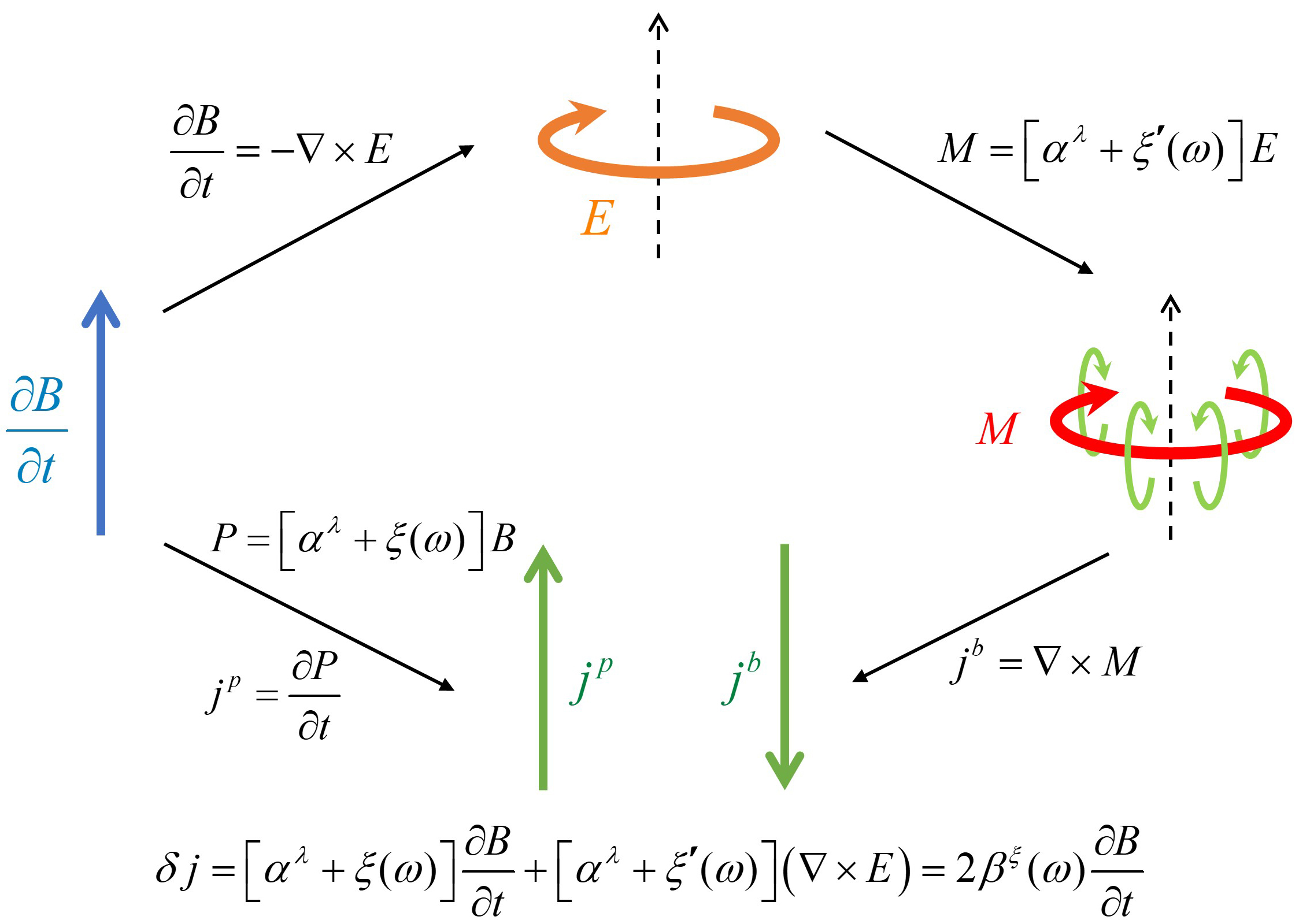
Figure 1: Microscopic process of dynamical magneto-electric effect. The schematic includes four parts: 1) polarization current $j^{p}$=$\partial_{t}\mathbf{P}$, with polarization $\mathbf{P}$ from magneto-electric coupling. 2) Faraday law $\partial_{t}\mathbf{B}=-\nabla\times\mathbf{E}$. 3) magneto-electric coupling induced magnetization $\mathbf{M}$. 4) bound current $j^{b}$=$\nabla\times\mathbf{M}$. The total current contains the polarization current $j^{p}$ and the bound current $j^{b}$. Due to the dynamical magneto-electric effect, the time-varying magnetic field can give rise to total dynamical magneto-electric current $\delta\mathbf{\bm{j}}^{\beta}=\left[\xi(\omega)-\xi^{\prime}(\omega)\right]\partial\mathbf{\mathbf{B}}/\partial t=2\beta(\omega)\partial\mathbf{\mathbf{B}}/\partial t$ with$\beta(\omega)=\left[\xi(\omega)-\xi^{\prime}(\omega)\right]/2$.

Considering a system with a longitudinal magneto-electric coupling, the total Lagrangian can be derived from the linear response theory and reads:

$$\mathscr{L}(t) = \frac{1}{2}\left[\varepsilon_{0}\mathbf{E}^{2}(t)-\frac{1}{\mu_{0}}\mathbf{B}^{2}(t)\right]-\rho\phi+\mathbf{j}\cdot\mathbf{A}$$ (1)

$$-\alpha^{\lambda}(t)\mathbf{E}(t)\cdot\mathbf{B}(t)-\mathbf{E}(t)\int\xi(t,t^{\prime})\mathbf{B}(t^{\prime})dt^{\prime}$$

$$-\mathbf{B}(t)\int\xi^{\prime}(t,t^{\prime})\mathbf{E}(t^{\prime})dt^{\prime},$$

which includes charge density $\rho$, electric potential $\phi$, current density $\mathbf{j}$, vector potential $\mathbf{A}$.The last three terms represent the magneto-electric response due to magneto-electric fields coupled with Bloch electrons in materials. Specifically, $\alpha^{\lambda}(t)$ denotes the simultaneous magneto-electric response, and $\xi(t,t^{\prime})$, $\xi^{\prime}(t,t^{\prime})$ represent the retarded magneto-electric response. In the following, we assume that the electric field $\mathbf{E}(t)=\mathbf{E_{0}^{\omega}}e^{-i\omega t}$ and magnetic field $\mathbf{B}(t)=\mathbf{B_{0}^{\omega}}e^{-i\omega t}$ are time-harmonic variables with frequency $\omega$. After Fourier transform from $t-t^{\prime}$ to $\omega$, the general charge response and current response can be derived from the Euler-Lagrange equations:

$$\delta\rho = -\nabla\left[\alpha^{\lambda}+\xi(\omega)\right]\cdot\mathbf{B}(t)$$ (2)

$$\delta\mathbf{j} = \nabla\left[\alpha^{\lambda}+\xi^{\prime}(\omega)\right]\times\mathbf{E}(t)+\partial_{t}\left[\alpha^{\lambda}+\xi(\omega)\right]\mathbf{B}(t)$$ (4)

$$+2\beta_{\omega}^{\xi}\partial_{t}\mathbf{B}(t)\,.$$

Here, the charge and current responses originate from magneto-electric effect are present, while the ordinary parts with $\rho_{0}\equiv\varepsilon_{0}\nabla\cdot\mathbf{E}(t)$ and $\mathbf{j}_{0}=-\varepsilon_{0}\partial_{t}\mathbf{E}+\frac{1}{\mu_{0}}\nabla\times\mathbf{B}$ are omitted. Comparing with previous studies, the first term of current responses describes the surface half integer anomalous Hall effect in an Axion insulator (RN35, ; RN6, ), and the second term describes the dynamical axion effect (RN20, ; Zhang_2020, ). Both of these effects should be corrected by the retarded magneto-electric response $\xi$ and $\xi^{(\prime)}$. The third term represents the dynamical magneto-electric effect (DME) $\delta\mathbf{\bm{j}}^{\beta}=2\beta_{\omega}^{\xi}\partial_{t}\mathbf{\mathbf{B}}$ ($\beta_{\omega}^{\xi}=\left[\xi(\omega)-\xi^{\prime}(\omega)\right]/2$), which only depends on the anti-commutative correlation of the magnetization operator $\hat{\mathbf{M}}$ and the polarization operator $\hat{\mathbf{P}}$ . The main focus of this work is the dynamical magneto-electric effect driven by a time-varying magnetic field denoted by the third term in Eq. 4. As shown in the Fig. 1, for the topological magneto-electric response term $\alpha^{\lambda}$ (including the case of an Axion insulator), the polarization current $j^{p}$ and bound current $j^{b}$ cancel each other. Meanwhile, for the retarded magneto-electric responses $\xi$ and $\xi^{\prime}$, an dynamical magneto-electric current $\delta\mathbf{\bm{j}}^{\beta}=2\beta_{\omega}^{\xi}\partial_{t}\mathbf{\mathbf{B}}$ exists, which is a novel effect not studied before.

General magneto-electric response.

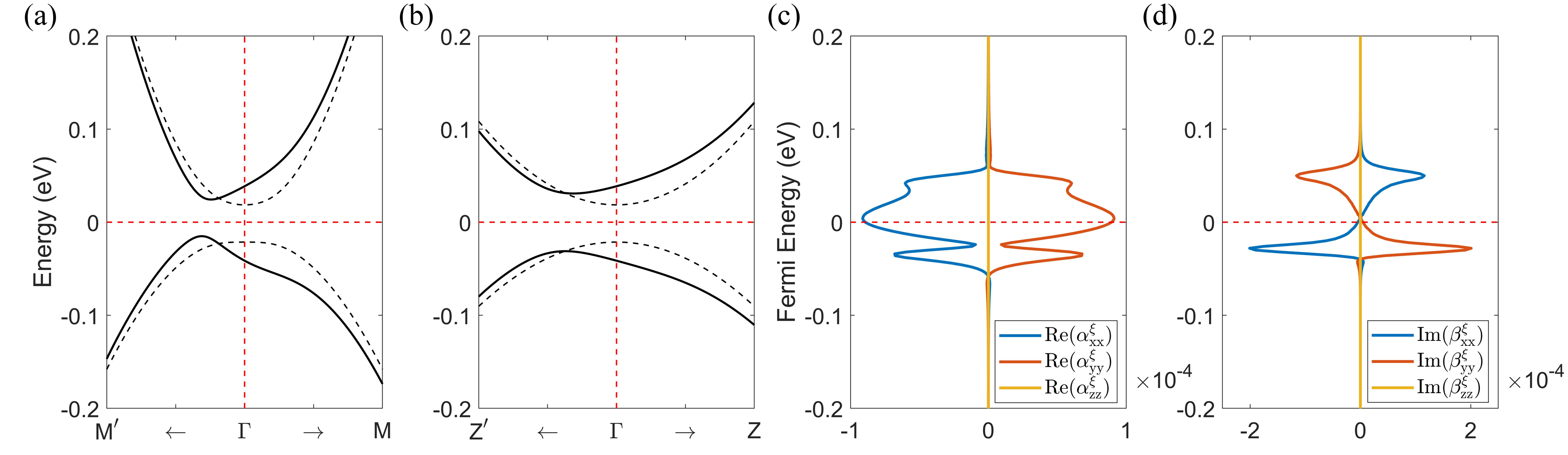
Figure 2: Effective model study of the retarded magneto-electric responses. The band-structure in (a) M direction and (b) Z direction. (c) commutative magneto-electric response $\alpha^{\xi}$ and (d) anti-commutative magneto-electric response $\beta^{\xi}$ ( in unit of $\bm{e}^{2}/\hbar$ ) ( $m_{1}=m_{2}=m_{3}=0.02$eV in $\delta H$ and $\hbar\omega=0.08$ eV ).

The general magneto-electric response can be obtained from the linear response theory (PhysRevB.99.045121, ), including both the simultaneous magneto-electric response $\alpha^{\lambda}(t,t)$ and the retarded magneto-electric response $\xi(t,t^{\prime})$ and $\xi^{\prime}(t,t^{\prime})$. The operator forms of these coefficients read as follows:

$$\alpha^{\lambda}(t,t) = -<|\frac{\partial^{2}H}{\partial\mathbf{E}\partial\mathbf{B}}|>_{0}\equiv\alpha^{\lambda}(t)$$ (5)

$$\xi(t,t^{\prime}) = -\frac{i}{\hbar}\Theta(t-t^{\prime})<|\left[\hat{\mathbf{P}}(t),\hat{\mathbf{M}}(t^{\prime})\right]|>_{0}$$ (6)

$$\xi^{\prime}(t,t^{\prime}) = -\frac{i}{\hbar}\Theta(t-t^{\prime})<|\left[\hat{\mathbf{M}}(t),\hat{\mathbf{P}}(t^{\prime})\right]|>_{0}\,,$$ (7)

where $\hat{\mathbf{P}}=-\partial H/\partial\mathbf{E}$ is the polarization operator, and $\hat{\mathbf{M}}=-\partial H/\partial\mathbf{B}$ is the orbital magnetization operator. The time variable $t$ in the brackets represents the measurement time, and $t^{\prime}$ represents the time of an external electric or a magnetic field. Then, the first term $\alpha^{\lambda}(t,t)$ is a response function at the same time, and the Maxwell relations in $\alpha^{\lambda}(t,t)$ make $\mathbf{B}$ and $\mathbf{E}$ commutative in relevant Lagrangian $\mathscr{L}^{\lambda}=-\alpha^{\lambda}(t)\mathbf{E}(t)\cdot\mathbf{B}(t)$. Thus, $\alpha^{\lambda}(t)$ represents the commutative magneto-electric response. The second term and the third term describe the magneto-electric response with different times, $\mathbf{P}(t)=\int\xi(t,t^{\prime})\mathbf{B}(t^{\prime})dt^{\prime},\mathbf{M}(t)=\int\xi^{\prime}(t,t^{\prime})\mathbf{E}(t^{\prime})dt^{\prime}$, and the related Lagrangian can be written as $\mathscr{L}^{\xi}(t)=-\int\left[\mathbf{E}(t)\xi(t,t^{\prime})\mathbf{B}(t^{\prime})+\mathbf{B}(t)\xi^{\prime}(t,t^{\prime})\mathbf{E}(t^{\prime})\right]dt^{\prime}$, where $\mathbf{B}$ and $\mathbf{E}$ are not commutative necessarily, for different times.

Comparing to notations of the optical conductivity in the linear response theory (PhysRevB.99.045121, ), $\alpha^{\lambda}(t)$ term is the intra-band Drude term, which also includes the Chern-Simons Axion term $\alpha^{\lambda}=\left(\bm{e}^{2}/2\pi h\right)\theta$ (Malashevich_2010, ). As for the retarded magneto-electric responses $\xi(t,t^{\prime})$ and $\xi^{\prime}(t,t^{\prime})$, the explicit formula can be obtained similar to the current-current correlation in the Kubo formula. To be specific, after Fourier transform from $t-t^{\prime}$ to frequency $\omega$, these coefficients read:

$$\xi_{ij}(\omega) = \bm{e}\int\frac{d\bm{k}}{(2\pi)^{3}}\sum_{n\neq m}\frac{\left(f_{nk}-f_{mk}\right)A_{nm}^{i}M_{mn}^{j}}{\varepsilon_{nk}-\varepsilon_{mk}+\hbar\omega+\mathrm{i}\eta}$$ (8)

$$\xi_{ji}^{\prime}(\omega) = \bm{e}\int\frac{d\bm{k}}{(2\pi)^{3}}\sum_{n\neq m}\frac{\left(f_{nk}-f_{mk}\right)M_{nm}^{j}A_{mn}^{i}}{\varepsilon_{nk}-\varepsilon_{mk}+\hbar\omega+\mathrm{i}\eta}$$ (9)

where $A_{mn}^{i}=iv_{mn}^{i}/\left(\varepsilon_{nk}-\varepsilon_{mk}\right)$ and $M_{nm}^{j}=\frac{e}{2}\sum_{l\neq m}\left(\bm{v}_{nl}\times\bm{A}_{lm}\right)^{j}$ are the inter-band elements of the Berry connection and the orbital magnetization in the basis of the eigen-functions with the eigen-energies $\varepsilon_{nk}$(gao2019semiclassical, ). In the following, we mainly consider the longitudinal retarded magneto-electric coefficients $\xi_{ii}(\omega)$ and $\xi_{ii}^{\prime}(\omega)$, and the transverse part is beyond the scope of this work. For convenience, one can separate the commutative part $\alpha_{ii}^{\xi}(\omega)$ and the anti-commutative part $\beta_{ii}^{\xi}(\omega)$ as follows:

$$\alpha_{ii}^{\xi}(\omega)=\left[\xi_{ii}(\omega)+\xi_{ii}^{\prime}(\omega)\right]/2$$

$$= \bm{e}\int\frac{d\bm{k}}{(2\pi)^{3}}\sum_{n\neq m}\frac{\left(-i\right)\left(f_{nk}-f_{mk}\right)v_{nm}^{i}M_{mn}^{i}}{\left(\varepsilon_{nk}-\varepsilon_{mk}\right)^{2}-\left(\hbar\omega\right)^{2}}$$

$$\beta_{ii}^{\xi}(\omega)=\left[\xi_{ii}(\omega)-\xi_{ii}^{\prime}(\omega)\right]/2$$

$$= \bm{e}\int\frac{d\bm{k}}{(2\pi)^{3}}\sum_{n\neq m}\frac{-\hbar\omega\left(f_{nk}-f_{mk}\right)A_{nm}^{i}M_{mn}^{i}}{\left(\varepsilon_{nk}-\varepsilon_{mk}\right)^{2}-\left(\hbar\omega\right)^{2}}\,,$$

where one can see that $\alpha_{ii}^{\xi}(\omega)$ is real while $\beta_{ii}^{\xi}(\omega)$ is purely imaginary .The anti-commutative magneto-electric coefficient $\beta_{\omega}^{\xi}$ can give rise to new kind of magneto-electric response, which manifests in systems without the time-reversal symmetry, the inversion symmetry and the mirror symmetry.

A simple effective model.

As shown in Eq.8, $\xi(\omega)$ is an inter-band gauge-independent term (similar to $\alpha_{ii}^{\xi}(\omega)$ and $\beta_{ii}^{\xi}(\omega)$), which is nonzero if the time-reversal symmetry $\mathscr{T}$ and the inversion symmetry $\mathscr{P}$ of the system are broken, unlike the Chern-Simons Axion term . Besides, other possible symmetries such as the mirror symmetry $\mathscr{M}_{x/y/z}$ should also be broken.

Here we would like to start from a well-known simple model to discuss the non-zero anti-commutative magneto-electric coefficient $\beta$. We adopt the Bi₂Se₃ effective model discussed in Ref.(zhang2009topological, ; RN20, ) with the basis of bonding and anti-bonding states of the p_z orbitals :

$$H = H_{0}+\delta H$$ (12)

$$H_{0} = \epsilon_{0}(k)+\sum_{a=1}^{5}d_{a}(k)\Gamma^{a}$$ (13)

$$\delta H = \sum_{i}^{1,2,3,5}m_{i}\Gamma^{i}\,,$$ (14)

where $\epsilon_{0}(k)=C+2D_{1}+4D_{2}-2D_{1}\mathrm{cos}k_{z}-2D_{2}(\mathrm{cos}k_{x}+\mathrm{cos}k_{y})$, $d_{1,2,3,4,5}=(A_{2}\mathrm{sin}k_{x},A_{2}\mathrm{sin}k_{y},A_{1}\mathrm{sin}k_{z},M(k),0)$, $M(k)=M-2B_{1}-4B_{2}+2B_{1}\mathrm{cos}k_{z}+2B_{2}(\mathrm{cos}k_{x}+\mathrm{cos}k_{y})$ and the Dirac matrixes $\Gamma^{1,2,3,4,5}=(\sigma_{x}\otimes s_{x},\sigma_{x}\otimes s_{y},\sigma_{y}\otimes s_{0},\sigma_{z}\otimes s_{0},\sigma_{x}\otimes s_{z})$ in the basis of ($\left|P1_{z}^{+},\uparrow\right\rangle$, $\left|P1_{z}^{+},\downarrow\right\rangle$, $\left|P2_{z}^{-},\uparrow\right\rangle$, $\left|P2_{z}^{-},\downarrow\right\rangle$). Here we choose the parameters ultilized previously by Zhang et al. with $A_{1}=0.4$, $A_{2}=0.8$, $B_{1}=2$, $B_{2}=11.32$, $C=-0.0014$, $D_{1}=0.26$, $D_{2}=3.92$, $M=0.02$(zhang2009topological, ; RN20, ). $H_{0}$ preserves both the time-reversal symmetry $\mathscr{T}$ and the inversion symmetry $\mathscr{P}$, while $\delta H$ breaks $\mathscr{T}$ and $\mathscr{P}$ but preserves the combinational symmetry $\mathscr{\mathscr{P}T}$. Also, $\delta H$ breaks the mirror symmetry $\mathscr{M}_{x/y/z}$, which may induce a non-zero anti-commutative magneto-electric response $\beta$.

As we can see in Fig.2 (a) & (b), the band structure of $H_{0}$ ( black dashed lines ) is an even function of the momentum k because of the $\mathscr{P}$ , $\mathscr{T}$ and the mirror symmetry. When the $\delta H$ is considered, these symmetries are broken, resulting in asymmetric band structure ( solid lines in Fig.2 (a) & (b) ). The symmetry breaking terms are associated with the factors of $\Gamma^{1,2,3}$ in the Hamiltonian $H$. In $H_{0}$, $d_{1,2,3}=(A_{2}\mathrm{sin}k_{x},A_{2}\mathrm{sin}k_{y},A_{1}\mathrm{sin}k_{z})$ are odd in $k_{x}$, $k_{y}$ and $k_{z}$ , respectively. However, $m_{1,2,3}$ in $\delta H$ are $\bm{k}$-independant constants. Thus, $m_{1,2,3}$ in $\delta H$ break the symmetries of $\mathscr{P}$ , $\mathscr{T}$ and mirror $\mathscr{M}_{x/y/z}$. Meanwhile, non-zero retarded magneto-electric response $\alpha_{ii}^{\xi}(\omega)$ and $\beta_{ii}^{\xi}(\omega)$ appear, as shown in Fig.2 (c) & (d). Importantly, $\beta_{xx}^{\xi}$ and $\beta_{yy}^{\xi}$ have the peak values around the band edges, while decrease to zero when Fermi energy locates in the band gap. In retrospect, the values of $\alpha_{xx}^{\xi}$ and $\alpha_{yy}^{\xi}$ shows peak values when Fermi energy locates in the band gap, and decrease when Fermi surface increases. The prominent values of $\beta_{xx}^{\xi}$ and $\beta_{yy}^{\xi}$ around the band edge can be explained from the remarkable asymmetric band structure around the band edge as shown in Fig.2 (a) & (b). With increasing the Fermi energy, $H_{0}$ becomes dominant and $\alpha_{ii}^{\xi}(\omega)$ and $\beta_{ii}^{\xi}(\omega)$ decrease as shown in Fig.2 (c) & (d).

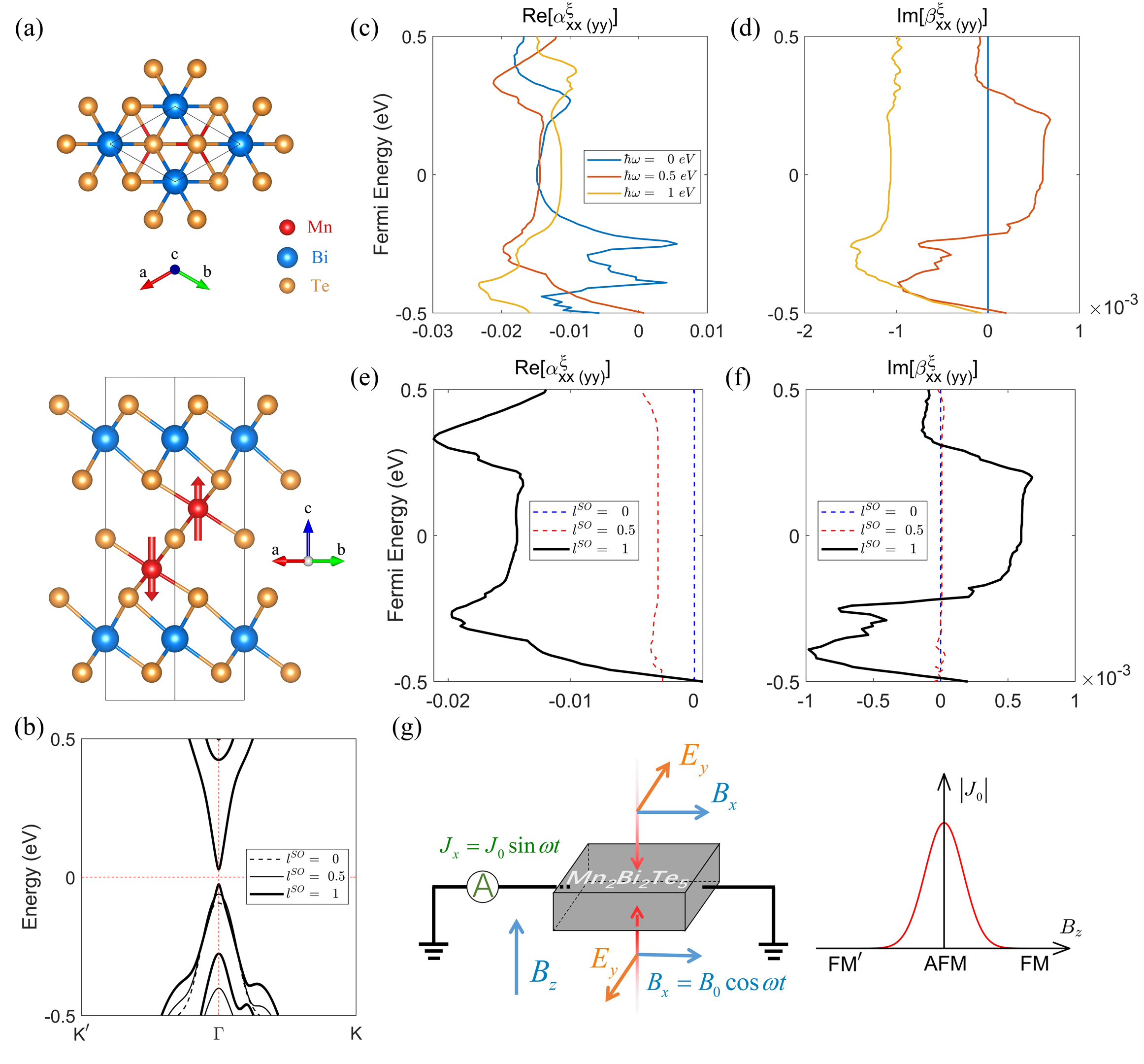
Figure 3: Result of Mn₂Bi₂Te₅: (a) Crystal structure and (b) the band-structures with different SOC strength $l^{SO}$ of Mn₂Bi₂Te₅. (c) - (d) magneto-electric response $\alpha_{xx(yy)}^{\xi}(\omega)$ and $\beta_{xx(yy)}^{\xi}(\omega)$ ( in unit of $\bm{e}^{2}/\hbar$ ) with different energy $\hbar\omega$ ( $l^{SO}$ = 1 ). (e) - (f) $\alpha_{xx(yy)}^{\xi}(\omega)$ and $\beta_{xx(yy)}^{\xi}(\omega)$ ( in unit of $\bm{e}^{2}/\hbar$ ) with SOC strength $l^{SO}$( $\hbar\omega$ = 0.5 eV ). The effective SOC strength $\widetilde{\lambda^{SO}}$ satisfies $\widetilde{\lambda^{SO}}=l^{SO}*\lambda^{SO}$, and $l^{SO}=1$ represents the case of original SOC strength $\lambda^{SO}$. Here $\alpha(\beta)_{xx}^{\xi}$ is equal to $\alpha(\beta)_{yy}^{\xi}$ due to $\mathscr{C}_{3z}$ symmetry. (g) An experiment setup for observation of DME.

A material candidate.

Based on the aforementioned model study of the dynamical magneto-electric response $\beta^{\xi}(\omega)$, the system with nonzero $\beta^{\xi}(\omega)$ needs to break the $\mathscr{P}$ , $\mathscr{T}$ and the mirror symmetry, and consequently possesses asymmetric band structure. Here we choose the ternary chalcogenide material Mn₂Bi₂Te₅ as an example. The space group of nonmagnetic Mn₂Bi₂Te₅ is $P\bar{3}m1$ ( No. 164 ) with symmetric operators $\mathscr{P}$ , $\mathscr{T}$, $\mathscr{M}_{x}$, $\mathscr{C}_{3z}$ and $\mathscr{C}_{2x}$ (the crystal structure of Mn₂Bi₂Te₅ is shown in Fig.3 (a) )(Zhang_2020, ; PhysRevB.104.054421, ) . When the antiferromagnetic order in 001 direction is considered, a non-zero $\beta^{\xi}(\omega)$ exists in this system. In Fig.3 (b), we plot the band structures of Mn₂Bi₂Te₅ with different values of spin orbital coupling (SOC) strength $\widetilde{\lambda^{SO}}=l^{SO}*\lambda^{SO}$, where $l^{SO}=1$ represents the case of original SOC strength $\lambda^{SO}$. When $l^{SO}=0$, the band is symmetric. As the SOC strength increases, symmetry breaking of $\mathscr{M}_{x}$ in orbital space occurs due to the SOC effect, resulting in an asymmetric band structure. Meanwhile, with increasing of the SOC strength, the values of $\alpha_{ii}^{\xi}(\omega)$ and $\beta_{ii}^{\xi}(\omega)$ become larger. As we can see in Fig.3 (b), the $\bm{k}$-path of $\Gamma$ - $\mathrm{K}$ and $\Gamma$ - $\mathrm{K^{\prime}}$ show obvious differences from -0.5 eV to -0.4 eV, resulting in rapidly changing of $\alpha_{ii}^{\xi}(\omega)$ and $\beta_{ii}^{\xi}(\omega)$ in Fig.3 (c) & (d). When the chosen Fermi Energy is increased to around zero, since the band asymmetry becomes less obvious, the change of $\alpha_{ii}^{\xi}(\omega)$ and $\beta_{ii}^{\xi}(\omega)$ become slow, and show plateau in the gap. Besides, the values of $\alpha_{ii}^{\xi}(\omega)$ and $\beta_{ii}^{\xi}(\omega)$ in the gap depend on the system parameters such as $l^{SO}$, as shown in Fig.3 (e) & (f). Moreover, with increasing of SOC’s strength $l^{SO}$, the energy bands become more asymmetric, and the values of $\alpha_{ii}^{\xi}(\omega)$’s and $\beta_{ii}^{\xi}(\omega)$’s are getting larger, as shown in Fig.3 (e) & (f). According to Ref. (Zhang_2020, ), the band structures of Mn₂Bi₂Te₅ are gapless around $l^{SO}=0.9$, and band inversion shows up at larger $l^{SO}$, which indicates that $\alpha_{ii}^{\xi}(\omega)$ and $\beta_{ii}^{\xi}(\omega)$ can be enhanced in topological materials with band inversion. Specifically, if $l^{SO}=0$, the inter-band matrix elements is small, such as $A_{nm}^{i}$ in Eq. General magneto-electric response., due to two bands near Fermi energy are from different atoms (Bi and Te). When $l^{SO}>0.9$(Zhang_2020, ), the band inversion shows up, which make P_z orbital of Bi and Te mixing, which enhances inter-band matrix elements in Eq. General magneto-electric response., and gives rise to a large magneto-electric response term $\beta^{\xi}(\omega)$. Also, as one can see in Eq. General magneto-electric response. & General magneto-electric response., $\hbar\omega$ is comparable with the band gap, so the materials with a small band gap are better for observing the dynamical magneto-electric response.

An experiment design.

Finally, we propose an experimental setup to detect the DME current $\delta\mathbf{\bm{j}}^{\beta}=2\mathbf{\beta}\partial_{t}\mathbf{\mathbf{B}}$. In Fig.3 (g), by adding an alternating magnetic field $\mathrm{B}_{x}$ in the x-direction, one can measure an alternating current in the same direction. The magnetic field $\mathrm{B}_{x}$ can be obtained from two light fields with different transmission directions, such the electric fields of which will cancel each other out (The thickness of the system should be smaller than the wavelength of the light fields). According to Ref. (Zhang_2020, ), the 001-antiferromagntic state is the ground state of Mn₂Bi₂Te₅, so we can observe a non-zero alternating current $J_{x}$ induced by alternating magnetic fields $\mathrm{B}_{x}$. Furthermore, if we add a large external static magnetic fields $\mathrm{B}_{z}$ in z-direction and shift Mn₂Bi₂Te₅ to FM state, the inversion symmetry $\mathscr{P}$ will become preserved and the anti-commutative magneto-electric response $\beta_{ii}^{\xi}(\omega)$ will vanish. Consequently, there will be no alternating current $J_{x}$ at a large external static magnetic field $\mathrm{B}_{z}$, as shown in Fig.3 (g). For example, if we have an experimental sample of cross-section size 1 $\mu$m² in x-direction with $\beta_{xx}^{\xi}\sim 0.001\left(\bm{e}^{2}/\hbar\right)$, and use 1T alternating magnetic field with 1 eV$/h$ frequency, we can detect an alternating current response of $\sim$ 100 $\mu$A.

Conclusion.

In summary, we find an anti-commutative magneto-electric response term $\beta^{\xi}(\omega)$, which can give rise to DME represented by $\delta\mathbf{\bm{j}}^{\beta}=2\mathbf{\beta}\partial_{t}\mathbf{\mathbf{B}}$. This novel magneto-electric response originates from the retarded magneto-electric response, and the microscopic coefficients are obtained from the linear response theory. Moreover, the characteristics of this DME are analyzed by a detailed four-band model, and we find that a non-zero $\beta^{\xi}(\omega)$ term exists in the systems without the time-reversal, inversion and the mirror symmetries. The values of $\beta^{\xi}(\omega)$ can be increased by raising the value of SOC, which gives rise to a prominent asymmetric band structure. Finally, we predict Mn₂Bi₂Te₅ as a material candidate and propose an experimental setup to observe the DME current, for the band inversion of Mn₂Bi₂Te₅ enhances magneto-electric response term $\beta^{\xi}(\omega)$.

Maoyuan Wang thanks Jin Cao for helpful discussion. This work was supported by the Strategic Priority Research Program of Chinese Academy of Sciences (Grant No. XDB28000000), the National Basic Research Program of China (Grants No. 2015CB921102, and No. 2017YFA0303301), the National Natural Science Foundation of China (Grant No. 12022407), and the China Postdoctoral Science Foundation (Grant No. 2021M700255).

Supplemental Materials for “Anti-commutative dynamical magneto-electric response in certain solid state materials”

.1 Formula derivation of Euler-Lagrange equations

We starts from the Lagrangian with retarded longitudinal magneto-electric coupling

$$L(\mathbf{r},t) = \frac{1}{2}\left[\varepsilon_{0}\mathbf{E}^{2}(\mathbf{r},t)-\frac{1}{\mu_{0}}\mathbf{B}^{2}(\mathbf{r},t)\right]-\rho\phi+\mathbf{j}\cdot\mathbf{A}-\alpha^{\lambda}(\mathbf{r})\mathbf{E}(\mathbf{r},t)\cdot\mathbf{B}(\mathbf{r},t)$$ (S1)

$$-\mathbf{E}(t)\int\xi(t,t^{\prime})\mathbf{B}(t^{\prime})dt^{\prime}-\mathbf{B}(t)\int\xi^{\prime}(t,t^{\prime})\mathbf{E}(t^{\prime})dt^{\prime}$$

which includes charge density $\rho$, electric potential $\phi$, current density $\mathbf{j}$, vector potential $\mathbf{A}$, simultaneous magneto-electric response $\alpha^{\lambda}(t)$ and retarded magneto-electric response $\xi(t,t^{\prime})$, $\xi^{\prime}(t,t^{\prime})$ . In the following, the space $\mathbf{r}$ dependence of the field are not shown for a shorted formula.Combing with relations from Maxwell equations

$$\mathbf{B}(t) = \nabla\times\mathbf{A}(t)$$ (S2)

$$\mathbf{E}(t) = -\nabla\phi(t)-\dot{\mathbf{A}}(t),$$ (S3)

one can obtain

$$L(t) = \frac{1}{2}\sum_{i}\varepsilon_{0}\left[\left(\partial_{i}\phi\right)^{2}+\left(\partial_{t}\mathbf{\mathrm{A}}_{i}\right)^{2}+2\partial_{t}\mathbf{\mathbf{\mathrm{A}}}_{i}\cdot\partial_{i}\phi\right]-\frac{1}{\mu_{0}}\sum_{i}\left[\left(\nabla\mathbf{\mathrm{A}}_{i}\right)^{2}-\partial_{i}\mathbf{A}\cdot\nabla\mathbf{\mathrm{A}}_{i}\right]+\left(-\rho\phi+\mathbf{j}\cdot\mathbf{A}\right)$$

$$-\alpha^{\lambda}\left(-\nabla\phi(t)-\dot{\mathbf{A}}(t)\right)\cdot\left(\nabla\times\mathbf{A}(t)\right)-\left(-\nabla\phi(t)-\dot{\mathbf{A}}(t)\right)\int\xi(t-t^{\prime})\mathbf{B}(t^{\prime})dt^{\prime}-\left(\nabla\times\mathbf{A}(t)\right)\int\xi^{\prime}(t-t^{\prime})\mathbf{E}(t^{\prime})dt^{\prime}.$$

Then, using Euler-Lagrange equations for scalar potential,

$$\frac{\partial L}{\partial\phi} = \partial_{t}(\frac{\partial L}{\partial\dot{\phi}})+\nabla\cdot\frac{\partial L}{\partial\left(\nabla\phi\right)},$$ (S5)

where

$$\frac{\partial L}{\partial\phi} = -\rho$$ (S6)

$$\frac{\partial L}{\partial\dot{\phi}} = 0$$ (S7)

$$\frac{\partial L}{\partial\left(\nabla\phi(t)\right)} = -\varepsilon_{0}\mathbf{E}(t)+\alpha^{\lambda}\left(\nabla\times\mathbf{A}(t)\right)+\int\xi(t-t^{\prime})\mathbf{B}(t^{\prime})dt^{\prime}$$ (S8)

$$\nabla\cdot\frac{\partial L}{\partial\left(\nabla\phi\right)} = -\varepsilon_{0}\nabla\cdot\mathbf{E}(t)+\left[\nabla\cdot\alpha^{\lambda}\right]\cdot\left(\nabla\times\mathbf{A}(t)\right)+\nabla\cdot\int\xi(t-t^{\prime})\mathbf{B}(t^{\prime})dt^{\prime}$$ (S9)

one can obtain

$$\frac{\partial L}{\partial\phi} = \partial_{t}(\frac{\partial L}{\partial\dot{\phi}})+\nabla\cdot\frac{\partial L}{\partial\left(\nabla\phi\right)}$$ (S10)

$$-\rho = -\varepsilon_{0}\nabla\cdot\mathbf{E}(t)+\left[\nabla\cdot\alpha^{\lambda}\right]\cdot\left(\nabla\times\mathbf{A}(t)\right)+\nabla\cdot\int\xi(t-t^{\prime})\mathbf{B}(t^{\prime})dt^{\prime}.$$ (S11)

In general, we know that free charge density $\rho_{0}\equiv\varepsilon_{0}\nabla\cdot\mathbf{E}(t)$, thus we can get extra charge density response from magnetic field

$$\delta\rho = \rho-\rho_{0}$$

$$= -\left[\nabla\cdot\alpha^{\lambda}\right]\cdot\mathbf{B}(t)-\int\left[\nabla\xi(t-t^{\prime})\right]\cdot\mathbf{B}(t^{\prime})dt^{\prime}.$$

Moreover, considering the Euler-Lagrange equations for vector potential

$$\frac{\partial L}{\partial\mathbf{\mathrm{A}}_{k}} = \partial_{t}(\frac{\partial L}{\partial\mathbf{\mathrm{\dot{A}}}_{k}})+\nabla\cdot\frac{\partial L}{\partial\left(\nabla\mathbf{\mathrm{A}}_{k}\right)},$$ (S13)

where

$$\frac{\partial L}{\partial\mathbf{\mathrm{A}}_{k}} = \mathrm{j}_{k}$$ (S14)

$$\frac{\partial L}{\partial\mathbf{\mathrm{\dot{A}}}_{k}} = \varepsilon_{0}\left(\mathbf{\mathrm{\dot{A}}}_{k}+\partial_{k}\phi\right)+\partial_{t}\left\{\alpha^{\lambda}\left[\mathbf{B}(t)\right]_{k}\right\}+\partial_{t}\left\{\int\xi(t-t^{\prime})\left[\mathbf{B}(t^{\prime})\right]_{k}dt^{\prime}\right\}$$ (S15)

$$\nabla\cdot\frac{\partial L}{\partial\left(\nabla\mathbf{\mathrm{A}}_{k}\right)} = -\nabla\cdot\varepsilon_{0}\left(\nabla\mathbf{\mathrm{A}}_{k}-\partial_{k}\mathbf{A}\right)+\left\{\nabla\times\left[\alpha^{\lambda}\mathbf{E}(t)\right]\right\}_{k}+\left\{\nabla\times\int\xi^{\prime}(t-t^{\prime})\mathbf{E}(t^{\prime})dt^{\prime}\right\}_{k},$$ (S16)

one can obtain

$$\mathbf{j} = -\varepsilon_{0}\partial_{t}\mathbf{E}+\frac{1}{\mu_{0}}\nabla\times\mathbf{B}+\partial_{t}\left[\alpha^{\lambda}\mathbf{B}(t)\right]+\partial_{t}\left[\int\xi(t-t^{\prime})\mathbf{B}(t^{\prime})dt^{\prime}\right]$$ (S17)

$$+\nabla\times\left[\alpha^{\lambda}\mathbf{E}(t)\right]+\nabla\times\int\xi^{\prime}(t-t^{\prime})\mathbf{E}(t^{\prime})dt^{\prime}.$$

Furthermore, based on the relation $\mathbf{j_{0}}\equiv-\varepsilon_{0}\partial_{t}\mathbf{E}+\frac{1}{\mu_{0}}\nabla\times\mathbf{B}$, then one can obtain the current response from magneto-electric response

$$\delta\mathbf{j} = \mathbf{j}-\mathbf{j}_{0}$$

$$= \partial_{t}\left[\alpha^{\lambda}\mathbf{B}(t)\right]+\partial_{t}\left[\int\xi(t-t^{\prime})\mathbf{B}(t^{\prime})dt^{\prime}\right]+\nabla\times\left[\alpha^{\lambda}\mathbf{E}(t)\right]+\nabla\times\int\xi^{\prime}(t-t^{\prime})\mathbf{E}(t^{\prime})dt^{\prime}$$

$$= \partial_{t}\alpha^{\lambda}\mathbf{B}(t)+\nabla\alpha^{\lambda}\times\mathbf{E}(t)+\partial_{t}\left[\int\xi(t-t^{\prime})\mathbf{B}(t^{\prime})dt^{\prime}\right]+\nabla\times\int\xi^{\prime}(t-t^{\prime})\mathbf{E}(t^{\prime})dt^{\prime},$$

Assuming the electric field and magnetic field is time-harmonic with frequency $\omega$, and Fourier transforming response function $\xi(t-t^{\prime})$ to $\xi(\omega^{\prime})$

$$\mathbf{B}(t^{\prime}) = \mathbf{B_{0}^{\omega}}e^{-i\omega t^{\prime}}$$ (S19)

$$\mathbf{E}(t^{\prime}) = \mathbf{E_{0}^{\omega}}e^{-i\omega t^{\prime}}$$ (S20)

$$\xi(t-t^{\prime}) = \frac{1}{2\pi}\int\xi(\omega^{\prime})e^{-i\omega^{\prime}(t-t^{\prime})}d\omega^{\prime},$$ (S21)

one can obtain

$$\delta\rho = \rho-\rho_{0}$$

$$= -\nabla\alpha^{\lambda}\cdot\mathbf{B}(t)-\int\left[\nabla\xi(t-t^{\prime})\right]\cdot\mathbf{B}(t^{\prime})dt^{\prime},$$

in which

$$\int\left[\nabla\cdot\xi(t-t^{\prime})\right]\cdot\mathbf{B}(t^{\prime})dt^{\prime} = \int\left[\nabla\int\xi(\omega^{\prime})e^{-i\omega^{\prime}(t-t^{\prime})}d\omega^{\prime}\right]\cdot\mathbf{B_{0}^{\omega}}e^{-i\omega t^{\prime}}dt^{\prime}$$ (S23)

$$= \frac{\mathbf{B_{0}^{\omega}}}{2\pi}\nabla\int\int\xi(\omega^{\prime})e^{-i(\omega-\omega^{\prime})t^{\prime}}dt^{\prime}d\omega^{\prime}$$

$$\nabla\xi(\omega)\cdot\mathbf{B_{0}^{\omega}}e^{-i\omega t},$$

thus one can obtain the charge density response

$$\delta\rho = -\nabla\alpha^{\lambda}\cdot\mathbf{B}(t)-\nabla\xi(\omega)\cdot\mathbf{B}(t)$$

$$= -\nabla\alpha^{\lambda}\cdot\mathbf{B}(t)-\nabla\left(\alpha_{\omega}^{\xi}+\beta_{\omega}^{\xi}\right)\cdot\mathbf{B}(t).$$

As for current response from in Eq..1, where

$$\partial_{t}\left[\int\xi(t-t^{\prime})\mathbf{B}(t^{\prime})dt^{\prime}\right] = \partial_{t}\left[\int\frac{1}{2\pi}\int\xi(\omega^{\prime})e^{-i\omega^{\prime}(t-t^{\prime})}d\omega^{\prime}\mathbf{B_{0}^{\omega}}e^{-i\omega t^{\prime}}dt^{\prime}\right]$$

$$= \mathbf{B_{0}^{\omega}}\partial_{t}\left[\int\frac{e^{-i\omega^{\prime}t}}{2\pi}\int\xi(\omega^{\prime})e^{-i(\omega-\omega^{\prime})t^{\prime}}dt^{\prime}d\omega^{\prime}\right]$$

$$= \mathbf{B_{0}^{\omega}}\partial_{t}\left[\int\frac{e^{-i\omega^{\prime}t}}{2\pi}\int\xi(\omega^{\prime})\delta(\omega-\omega^{\prime})d\omega^{\prime}\right]$$

$$= \partial_{t}\left[\mathbf{B_{0}^{\omega}}e^{-i\omega t}\xi(\omega)\right]$$

$$= \partial_{t}\left[\mathbf{B}(t)\xi(\omega)\right],$$ (S27)

one can obtain current response

$$\delta\mathbf{j} = \partial_{t}\alpha^{\lambda}\mathbf{B}(t)+\nabla\alpha^{\lambda}\times\mathbf{E}(t)+\partial_{t}\left[\mathbf{B}(t)\xi(\omega)\right]+\xi^{\prime}(\omega)\nabla\times\mathbf{E}(t)$$

$$= \partial_{t}\alpha^{\lambda}\mathbf{B}(t)+\nabla\alpha^{\lambda}\times\mathbf{E}(t)+\frac{\partial\left(\alpha_{\omega}^{\xi}+\beta_{\omega}^{\xi}\right)}{\partial t}\mathbf{B}(t)+\mathbf{\nabla}\left(\alpha_{\omega}^{\xi}-\beta_{\omega}^{\xi}\right)\times\mathbf{E}(t)+2\beta_{\omega}^{\xi}\partial_{t}\mathbf{B}(t).$$

$$= \partial_{t}\left(\alpha^{\lambda}+\alpha_{\omega}^{\xi}+\beta_{\omega}^{\xi}\right)\mathbf{B}(t)+\nabla\left(\alpha^{\lambda}+\alpha_{\omega}^{\xi}-\beta_{\omega}^{\xi}\right)\times\mathbf{E}(t)+2\beta_{\omega}^{\xi}\partial_{t}\mathbf{B}(t).$$

The current response is the central phenomenological relation for dynamical magneto-electric effect as shown in Eq. (3) of the main text. In the following, we give a microscopic derivation for the DME based on the linear response theory.

.2 Linear response theory of dynamical magneto-electric effect.

For a system $H_{0}$ with perturbations, the total Hamiltonian

$$H=H_{0}+V_{1}(t)+V_{2}(t)+\cdots,$$ (S29)

where n in $V_{n}$ marked the n-th order perturbation. And the equation of motion for density operator reads $i\hbar\dot{\rho}\left(t\right)=\left[H,\rho\right]$, where $\rho_{0}$ is the unperturbed density operator. According to standard perturbation procedure [39], we replace $\underset{n}{\sum}V_{n}(t)$ and $\rho$ with $\underset{n}{\sum}\lambda^{n}V_{n}(t)$ and $\underset{n}{\sum}\lambda^{n}\rho_{n}(t)$ in the equation of motion, and separate terms according to the order of $\lambda$, then we can get the equation of motion for different order of density operator:

$$i\hbar\dot{\rho}_{0} = \left[H_{0},\rho_{0}\right]$$ (S30)

$$i\hbar\dot{\rho}_{1}\left(t\right) = \left[H_{0},\rho_{1}\left(t\right)\right]+\left[V_{1}\left(t\right),\rho_{0}\right].$$ (S31)

Since the density operator here is in Schrï¿œdinger picture, it is convenient to utilize the interaction picture, $\rho^{I}\left(t\right)=e^{iH_{0}t}\rho(t)e^{-iH_{0}t}$. The equation of motion for density operator can be simplified as:

$$i\hbar\dot{\rho}_{0}^{I} = 0$$ (S32)

$$i\hbar\dot{\rho}_{1}^{I}\left(t\right) = \left[V_{1}^{I}\left(t\right),\rho_{0}^{I}\left(t\right)\right].$$ (S33)

After integral, the density operator can be simplified as:

$$\rho_{1}^{I}\left(t\right) = -\frac{i}{\hbar}\int_{-\infty}^{t}dt^{\prime}\,\left[V_{1}^{I}\left(t^{\prime}\right),\rho_{0}^{I}\right].$$ (S34)

For a response $R$ excited by an excitation $E$, $V$ , we can identify response function [39]:

$$\mathscr{F}^{\left(1\right)0}(t,t) = Tr\left[\rho_{0}(t)\frac{\partial\hat{R}(t)}{\partial E(t)}\right]$$

$$= <|\frac{\partial\hat{R}(t)}{\partial E(t)}|>_{0}$$

$$\mathscr{F}^{\left(1\right)1}(t,t^{\prime}) = \Theta_{t^{\prime}}^{t}Tr\left[\frac{\delta\rho_{1}^{I}(t)}{\delta V_{1}^{I}(t^{\prime})}\frac{\partial V_{1}^{I}(t^{\prime})}{\partial E(t^{\prime})}\hat{R}(t)\right]$$

$$= -\frac{i}{\hbar}\Theta_{t^{\prime}}^{t}<|\left[R(t),\frac{\partial V_{1}^{I}(t^{\prime})}{\partial E(t^{\prime})}\right]|>_{0},$$

where $\left(1\right)$ in $\mathscr{F}^{\left(1\right)0}(t,t)$ represent first order, and the second integer represent two different response functions. $\mathscr{F}^{\left(1\right)0}(t,t)$ is a simultaneous response function and $\mathscr{F}^{\left(1\right)1}(t,t^{\prime})$ is a retarded response function. For magneto-electric response, $R$ operator could be Polarization $\mathbf{P}$, excitation $E$ could be electric field $\mathbf{E}$, perturbation $V_{1}=-\mathbf{M}\cdot\mathbf{B}$, or $R$ operator could be magnetization operator $\mathbf{M}$, excitation $E$ could be electric field $\mathbf{\mathbf{B}}$, perturbation $V_{1}=-\mathbf{P}\cdot\mathbf{E}$.

For $\mathscr{F}^{\left(1\right)0}(t,t)$, we identify it as $\lambda(t,t)$,

$$\lambda(t,t) = <|\frac{\partial\hat{\mathbf{P}}}{\partial\mathbf{B}}|>_{0}=<|\frac{\partial\hat{\mathbf{M}}}{\partial\mathbf{E}}|>_{0}$$ (S37)

$$= -<|\frac{\partial^{2}H}{\partial\mathbf{E}\partial\mathbf{B}}|>_{0}\equiv\alpha^{\lambda}\,.$$

As for $\mathscr{F}^{\left(1\right)1}(t,t^{\prime})$, we have two functions:

$$\xi(t,t^{\prime}) = -\frac{i}{\hbar}\Theta(t-t^{\prime})<|\left[\hat{\mathbf{P}}(t),\hat{\mathbf{M}}(t^{\prime})\right]|>_{0}$$ (S38)

$$\xi^{\prime}(t,t^{\prime}) = -\frac{i}{\hbar}\Theta(t-t^{\prime})<|\left[\hat{\mathbf{M}}(t),\hat{\mathbf{P}}(t^{\prime})\right]|>_{0}\,,$$ (S39)

then we Fourier transform from $t-t^{\prime}$ to frequency $\omega$ in the bulk system with near equilibrium approximation:

$$\xi_{ij}(\omega=\omega_{1})$$

$$= \frac{1}{2\pi}\iint_{-\infty}^{+\infty}dtdt^{\prime}e^{i\omega t}\xi_{ij}(t,t^{\prime})$$

$$= \frac{-i}{2\pi\hbar}\int\frac{d\bm{k}}{(2\pi)^{d}}\iint_{-\infty}^{+\infty}dtdt^{\prime}e^{i(\omega t-\omega_{1}t^{\prime})}\Theta(t-t^{\prime})<|\left[\mathrm{P}_{i}\left(t\right),\mathrm{M}_{j}\left(t^{\prime}\right)\right]|>_{0}$$

$$= \frac{-i}{2\pi\hbar}\sum_{l,l^{\prime},m,m^{\prime}}\int\frac{d\bm{k}}{(2\pi)^{d}}\iint_{-\infty}^{+\infty}dtdt^{\prime}e^{i(\omega t-\omega_{1}t^{\prime})}\mathrm{P}_{ll^{\prime}}^{i}\mathrm{M}_{mm^{\prime}}^{j}\bm{\Theta(t-t^{\prime})<|\left[c_{l}^{\dagger}\left(t\right)c_{l^{\prime}}\left(t\right),c_{m}^{\dagger}\left(t^{\prime}\right)c_{m^{\prime}}\left(t^{\prime}\right)\right]|>_{0}}$$

$$= \frac{-i}{2\pi\hbar}\sum_{l,l^{\prime},m,m^{\prime}}\int\frac{d\bm{k}}{(2\pi)^{d}}\iint_{-\infty}^{+\infty}d(t-t^{\prime})dt^{\prime}e^{i\omega(t-t^{\prime})}e^{i(\omega-\omega_{1})t^{\prime}}\times$$

$$\,\,\,\,\,\,\,\,\,\,\,\,\,\,\,\,\,\,\,\,\,\,\,\,\,\,\mathrm{P}_{ll^{\prime}}^{i}\mathrm{M}_{mm^{\prime}}^{j}\left[\bm{g_{l^{\prime}m}^{r}(t-t^{\prime})g_{m^{\prime}l}^{<}(t^{\prime}-t)+g_{l^{\prime}m}^{<}(t-t^{\prime})g_{m^{\prime}l}^{a}(t^{\prime}-t)}\right]$$

$$= \frac{-i}{\left(2\pi\right)^{3}\hbar}\sum_{l,l^{\prime},m,m^{\prime}}\int\frac{d\bm{k}}{(2\pi)^{d}}\iint_{-\infty}^{+\infty}d(t-t^{\prime})dt^{\prime}\iint_{-\infty}^{+\infty}dE_{1}dE_{2}e^{-i(E_{1}-E_{2})(t-t^{\prime})/\hbar}e^{i\omega(t-t^{\prime})}e^{i(\omega-\omega_{1})t^{\prime}}\times$$

$$\,\,\,\,\,\,\,\,\,\,\,\,\,\,\,\,\,\,\,\,\,\,\,\,\,\,\mathrm{P}_{ll^{\prime}}^{i}\mathrm{M}_{mm^{\prime}}^{j}\left[g_{l^{\prime}m}^{r}(E_{1})g_{m^{\prime}l}^{<}(E_{2})+g_{l^{\prime}m}^{<}(E_{1})g_{m^{\prime}l}^{a}(E_{2})\right]$$

$$= \frac{-i}{2\pi}\sum_{l,l^{\prime},m,m^{\prime}}\iint\frac{d\bm{k}}{(2\pi)^{d}}dE_{2}\mathrm{P}_{ll^{\prime}}^{i}\mathrm{M}_{mm^{\prime}}^{j}\left[g_{l^{\prime}m}^{r}(E_{2}+\hbar\omega)g_{m^{\prime}l}^{<}(E_{2})+g_{l^{\prime}m}^{<}(E_{2}+\hbar\omega)g_{m^{\prime}l}^{a}(E_{2})\right]$$

$$= i\iint\frac{d\bm{k}}{(2\pi)^{d}}\frac{dE}{2\pi}f(E)Tr\left(\mathrm{P}^{i}g_{E+\hbar\omega}^{r}\mathrm{M}^{j}g_{E}^{r-a}+g_{E}^{r-a}\mathrm{M}^{j}g_{E-\hbar\omega}^{a}\mathrm{P}^{i}\right)$$

$$= \int\frac{d\bm{k}}{(2\pi)^{d}}\sum_{n\neq m}\frac{\left(f_{nk}-f_{mk}\right)\mathrm{P}_{nm}^{i}M_{mn}^{j}}{\varepsilon_{nk}-\varepsilon_{mk}+\hbar\omega+\mathrm{i}\eta},$$

where $g^{r},$$g^{a}$, $g^{<}$ are retarded, advanced, lesser Green’s functions, $g^{r-a}=g^{r}-g^{a}$, $\mathrm{P}_{nm}^{i}=\bm{e}r_{nm}^{i}=\bm{e}<nk|\hat{r}_{i}|mk>=\bm{e}<nk|i\partial_{k_{i}}|mk>=\bm{e}<nk|i\partial_{k_{i}}|mk>=\bm{e}A_{nm}^{i}$ is inter-band polarization, $A_{mn}^{i}=iv_{mn}^{i}/\left(\varepsilon_{nk}-\varepsilon_{mk}\right)$ is inter-band Berry connection, and $M_{nm}^{j}=\frac{\bm{e}}{2}\sum_{l\neq m}\left(\bm{v}_{nl}\times\bm{A}_{lm}\right)^{j}$ is inter-band elements of orbital magnetization[3, 4].

$$\xi_{ij}(\omega) = \bm{e}\int\frac{d\bm{k}}{(2\pi)^{d}}\sum_{n\neq m}\frac{\left(f_{nk}-f_{mk}\right)A_{nm}^{i}M_{mn}^{j}}{\varepsilon_{nk}-\varepsilon_{mk}+\hbar\omega+\mathrm{i}\eta}$$ (S41)

$$\xi_{ji}^{\prime}(\omega) = \bm{e}\int\frac{d\bm{k}}{(2\pi)^{d}}\sum_{n\neq m}\frac{\left(f_{nk}-f_{mk}\right)M_{nm}^{j}A_{mn}^{i}}{\varepsilon_{nk}-\varepsilon_{mk}+\hbar\omega+\mathrm{i}\eta}.$$ (S42)

Furthermore, we can get two diagonal response functions from linear combination of $\xi(\omega)$ and $\xi^{\prime}(\omega)$,

$$\alpha_{ii}^{\xi} = \left[\xi_{ii}(\omega)+\xi_{ii}^{\prime}(\omega)\right]/2$$

$$= \bm{e}\int\frac{d\bm{k}}{(2\pi)^{d}}\sum_{n\neq m}\frac{\left(f_{nk}-f_{mk}\right)A_{nm}^{i}M_{mn}^{i}}{\varepsilon_{nk}-\varepsilon_{mk}+\hbar\omega+\mathrm{i}\eta}$$

$$+\bm{e}\int\frac{d\bm{k}}{(2\pi)^{d}}\sum_{n\neq m}\frac{\left(f_{nk}-f_{mk}\right)M_{nm}^{i}A_{mn}^{i}}{\varepsilon_{nk}-\varepsilon_{mk}+\hbar\omega+\mathrm{i}\eta}$$

$$= \bm{e}\int\frac{d\bm{k}}{(2\pi)^{d}}\sum_{n\neq m}\frac{\left(f_{nk}-f_{mk}\right)A_{nm}^{i}M_{mn}^{i}}{\varepsilon_{nk}-\varepsilon_{mk}+\hbar\omega+\mathrm{i}\eta}$$

$$+\bm{e}\int\frac{d\bm{k}}{(2\pi)^{d}}\sum_{n\neq m}\frac{\left(f_{nk}-f_{mk}\right)A_{nm}^{i}M_{mn}^{i}}{\varepsilon_{nk}-\varepsilon_{mk}-\hbar\omega-\mathrm{i}\eta}$$

$$= \bm{e}\int\frac{d\bm{k}}{(2\pi)^{d}}\sum_{n\neq m}\frac{\left(f_{nk}-f_{mk}\right)\left(\varepsilon_{nk}-\varepsilon_{mk}\right)A_{nm}^{i}M_{mn}^{i}}{\left[\left(\varepsilon_{nk}-\varepsilon_{mk}\right)^{2}-\left(\hbar\omega+\mathrm{i}\eta\right)^{2}\right]}$$

$$= \bm{e}\int\frac{d\bm{k}}{(2\pi)^{d}}\sum_{n\neq m}\frac{\left(-i\right)\left(f_{nk}-f_{mk}\right)v_{nm}^{i}M_{mn}^{i}}{\left[\left(\varepsilon_{nk}-\varepsilon_{mk}\right)^{2}-\left(\hbar\omega+\mathrm{i}\eta\right)^{2}\right]}$$

$$\beta_{ii}^{\xi}(\omega) = \left[\xi_{ii}(\omega)-\xi_{ii}^{\prime}(\omega)\right]/2$$ (S44)

$$= \bm{e}\int\frac{d\bm{k}}{(2\pi)^{d}}\sum_{n\neq m}\frac{\left(f_{nk}-f_{mk}\right)A_{nm}^{i}M_{mn}^{i}}{\varepsilon_{nk}-\varepsilon_{mk}+\hbar\omega+\mathrm{i}\eta}$$

$$-\bm{e}\int\frac{d\bm{k}}{(2\pi)^{d}}\sum_{n\neq m}\frac{\left(f_{nk}-f_{mk}\right)M_{nm}^{i}A_{mn}^{i}}{\varepsilon_{nk}-\varepsilon_{mk}+\hbar\omega+\mathrm{i}\eta}$$

$$= \bm{e}\int\frac{d\bm{k}}{(2\pi)^{d}}\sum_{n\neq m}\frac{\left(f_{nk}-f_{mk}\right)A_{nm}^{i}M_{mn}^{i}}{\varepsilon_{nk}-\varepsilon_{mk}+\hbar\omega+\mathrm{i}\eta}$$

$$-\bm{e}\int\frac{d\bm{k}}{(2\pi)^{d}}\sum_{n\neq m}\frac{\left(f_{nk}-f_{mk}\right)A_{nm}^{i}M_{mn}^{i}}{\varepsilon_{nk}-\varepsilon_{mk}-\hbar\omega-\mathrm{i}\eta}$$

$$= \bm{e}\int\frac{d\bm{k}}{(2\pi)^{d}}\sum_{n\neq m}\frac{-\hbar\omega\left(f_{nk}-f_{mk}\right)A_{nm}^{i}M_{mn}^{i}}{\left[\left(\varepsilon_{nk}-\varepsilon_{mk}\right)^{2}-\left(\hbar\omega+\mathrm{i}\eta\right)^{2}\right]}.$$

These dynamical magneto-electric coefficients represent the main microscopic results of our work as shown in Eq. (8)-(9) of the main text.

Next, we discuss about gauge-relavant issues. Generally, gauge-dependence comes from partial differential operator, such as in Berry connection $A_{mm}^{i}=<mk|i\partial_{k_{i}}|mk>$. If we make a gauge transform $|\tilde{mk}>=e^{i\psi_{m}(k)}|mk>$,

$$\tilde{A}_{mm}^{i} = <\tilde{mk}|i\partial_{k_{i}}|\tilde{mk}>$$

$$= <mk|e^{-i\psi_{m}(k)}e^{i\psi_{m}(k)}\left(i\partial_{k_{i}}|mk>\right)+<mk|e^{-i\psi_{m}(k)}\left(i\partial_{k_{i}}e^{i\psi_{m}(k)}\right)|mk>$$

$$= <mk|i\partial_{k_{i}}|mk>-<mk|e^{-i\psi_{m}(k)}e^{i\psi_{m}(k)}\left(\partial_{k_{i}}\psi_{m}(k)\right)|mk>$$

$$= A_{mm}^{i}-\partial_{k_{i}}\psi_{m}(k)\,,$$

therefore the (intra-band) Berry connection depend on the phase $\psi(k)$ chose in the gauge.

However, for the inter-band Berry connection $A_{nm}^{i}=<nk|i\partial_{k_{i}}|mk>\,\left(n\neq m\right)$, the first term of different gauge is

$$<nk|e^{-i\psi_{n}(k)}e^{i\psi_{m}(k)}\left(i\partial_{k_{i}}|mk>\right)$$

$$= e^{i\left[\psi_{m}(k)-\psi_{n}(k)\right]}<nk|i\partial_{k_{i}}|mk>,\,\left(n\neq m\right)$$

and the second term is

$$<nk|e^{-i\psi(k)}e^{i\psi(k)}\left(\partial_{k_{i}}\psi(k)\right)|mk>$$ (S47)

$$= \left(\partial_{k_{i}}\psi(k)\right)<nk|mk>$$

$$= 0,\,\left(n\neq m\right)$$

due to the orthogonality of two states. Therefore, the interband Berry connection$\tilde{A}_{nm}^{i}=e^{i\left[\psi_{m}(k)-\psi_{n}(k)\right]}A_{nm}^{i}$. Similarly, interband orbital magnetization of different gauge is

$$\tilde{M}_{mn}^{j} = \frac{\bm{e}}{2}\sum_{l\neq n}\left(\bm{\tilde{v}}_{ml}\times\bm{\tilde{A}}_{ln}\right)^{j}$$

$$= \frac{\bm{e}}{2}\sum_{l\neq n}\left(\bm{v}_{ml}e^{i\left[\psi_{l}(k)-\psi_{m}(k)\right]}\times\bm{A}_{ln}e^{i\left[\psi_{n}(k)-\psi_{l}(k)\right]}\right)^{j}$$

$$= e^{i\left[\psi_{n}(k)-\psi_{m}(k)\right]}M_{mn}^{j}.$$

So, the inter-band Berry connection times interband orbital magnetization $\tilde{A}_{nm}^{i}\tilde{M}_{mn}^{j}=A_{nm}^{i}M_{mn}^{j}\,\left(n\neq m\right)$ in Eq. S41, Eq. S42 and Eq. S44 is gauge independent due to their two extra phases canceling each other, which explains that the magneto-electric response term $\beta$ is gauge-independent or gauge invariant.

.3 Symmetry analyses for magneto-electric coefficients

Magneto-electric response describes that an electric field can induce the magnetization $\mathbf{M}=a\mathbf{E}$ with a coefficient

$$a = \alpha-\beta$$ (49)

or a magnetic field can induce the polarization $\mathbf{P}=b\mathbf{B}$ with a coefficient

$$b = \alpha+\beta\,.$$ (50)

Using an inversion symmetry operation, we have

$$\mathscr{P}\left(\mathbf{E}\right) = -\mathbf{E}$$ (51)

$$\mathscr{P}\left(\mathbf{B}\right) = \mathbf{B}$$ (52)

$$\mathscr{P}\left(\mathbf{P}\right) = -\mathbf{\mathbf{P}}$$ (53)

$$\mathscr{P}\left(\mathbf{M}\right) = \mathbf{M},$$ (54)

and further

$$\mathscr{P}\left(\mathbf{M}\right) = \mathscr{P}\left(a\right)\mathscr{P}\left(\mathbf{E}\right)$$ (55)

$$\mathbf{M} = -\mathscr{P}\left(a\right)\mathbf{E}$$ (56)

for example. Combining $\mathbf{M}=a\mathbf{E}$ and $\mathbf{M}=-\mathscr{P}\left(a\right)\mathbf{E}$, we have $\mathscr{P}\left(a\right)=-a$, which indicates that in the system with the inversion symmetry, the gauge-independent coefficient $a=0$ (If $a$ is a gauge-dependent coefficient like Chern Simon term $\alpha^{CS}=\left(\bm{e}^{2}/2\pi h\right)\theta$, where $\theta\rightarrow\theta+2\pi n$ under gauge transform, the inversion symmetry make $\theta=\pi n$, where $n$ is an integer). As for coefficient $b$, since $\mathbf{\mathscr{P}\left(P\right)}=-\mathbf{\mathbf{P}}=\mathscr{P}\left(b\right)\mathbf{B}$, it is the same as $a$ with inversion symmetry. And if both $a$ and $b$ are zero, both $\alpha$ and $\beta$ are zero too. Generally, one can consider these coefficients as tensors, and diagonal coefficients $a_{ii}$, $b_{ii}$ and $\alpha_{ii}$, $\beta_{ii}$ also vanish in system with inversion symmetry similar to the case shown above. (offdiagonal magneto-electric coefficients $a_{ij}$ and $b_{ji}$ are not discussed in details in this work).

Similarly, using a time-reversal symmetry $\mathscr{T}$ operation,

$$\mathscr{T}\left(\mathbf{E}\right) = \mathbf{E}$$ (57)

$$\mathscr{T}\left(\mathbf{B}\right) = \mathbf{-B}$$ (58)

$$\mathscr{T}\left(\mathbf{P}\right) = \mathbf{\mathbf{P}}$$ (59)

$$\mathscr{T}\left(\mathbf{M}\right) = \mathbf{-M},$$ (60)

it has similar results that $\mathscr{T}\left(a\right)=-a,\mathscr{T}\left(b\right)=-b$.

Besides, mirror symmetry is also important, which usually has three operators $\mathscr{M}_{x/y/z}$. Using these operators, we have

$$\mathscr{M}_{i}\left(\mathrm{E}_{j}\right) = \left(-1\right)^{\delta_{ij}}\mathrm{E}_{j}$$ (61)

$$\mathscr{M}_{i}\left(\mathrm{B}_{j}\right) = \left(-1\right)^{1-\delta_{ij}}\mathrm{B}_{j}$$ (62)

$$\mathscr{M}_{i}\left(\mathrm{P}_{j}\right) = \left(-1\right)^{\delta_{ij}}\mathrm{P}_{j}$$ (63)

$$\mathscr{M}_{i}\left(\mathrm{M}_{j}\right) = \left(-1\right)^{1-\delta_{ij}}\mathrm{M}_{j},$$ (64)

where index i (j) represents vector component’s direction. For example, if we consider magneto-electric response $\mathrm{M}_{z}=a_{zz}\mathrm{E}_{z}$, $\mathrm{P}_{z}=b_{zz}\mathrm{B}_{z}$, the mirror operator $\mathscr{M}_{z}$ results in $\mathrm{M}_{z}=\mathscr{M}_{z}\left(a_{zz}\right)\left(-\mathrm{E}_{z}\right)$, $\left(-\mathrm{P}_{z}\right)=\mathscr{M}_{z}\left(b_{zz}\right)\mathrm{B}_{z}$, while the mirror operator $\mathscr{M}_{x/y}$ results in $\left(-\mathrm{M}_{z}\right)=\mathscr{M}_{x/y}\left(a_{zz}\right)\mathrm{E}_{z}$, $\mathrm{\mathrm{P}_{z}}=\mathscr{M}_{z}\left(b_{zz}\right)\left(-\mathrm{B}_{z}\right)$, which further makes $\mathscr{M}_{x/y/z}\left(a_{zz}\right)=-a_{zz}$, $\mathscr{M}_{x/y/z}\left(b_{zz}\right)=-b_{zz}$. Therefore, any mirror symmetry in one system will make gauge-independent diagonal magneto-electric coefficients $a_{ii}=0,\,b_{ii}=0$ (and further $\alpha_{ii}=0,\,\beta_{ii}=0$) (offdiagonal magneto-electric coefficients $a_{ij}$ and $b_{ji}$ can retain one mirror symmetry $\mathscr{M}_{j}$).

For the off-diagonal magneto-electric coefficients of the alpha and beta tensors $a_{ij}$ and $b_{ji}$, it is not relevant to our work, because we study the type of magneto-electric response like $E\cdot B$, which only involves diagonal magneto-electric coefficients $a_{ii}$ and $b_{ii}$ in the Lagrangian:

$$\mathscr{L}^{ME} = \sum_{i}B_{i}a_{ii}E_{i}+E_{i}b_{ii}B_{i}\,.$$ (65)

The off-diagonal magneto-electric coefficients involve in the magneto-electric response type like

$$\mathscr{L}^{ME} = \sum_{i\neq j}B_{i}a_{ij}E_{j}+E_{j}b_{ji}B_{i}\,,$$ (66)

which needs systematic study in further work.

.4 Calculation details for Mn₂Bi₂Te₅

The first-principles calculations for Mn₂Bi₂Te₅ are performed using Vienna ab initio simulation package (VASP) [45, 46] based on the density function theory with Perdew-Burke-Ernzerhof (PBE) parameterization of generalized gradient approximation (GGA)[47]. The energy cutoff of the plane wave basis is set as 300 eV, and the Brillouin zone is sampled by 12 × 12 × 4 k-mesh.

The magneto-electric coefficients are calculated based on the Hamiltonian of maximally localized Wannier functions (MLWF)[48] with s, d orbitals of Mn atoms, and s, p orbitals of Bi atoms and Te atoms, with 100 × 100 × 40 k-mesh in the Brillouin zone. To be more explicit, after MLWF calculations, we have MLWF Hamiltonian and position operator matrix

$$H_{ij}(R) = <0i|H|jR>$$ (67)

$$r_{ij}^{x/y/z}(R) = <0i|r^{x/y/z}|jR>\,,$$ (68)

where i, j represent MLWF orbitals, R represents cell vector and $r^{x/y/z}$ represents position operator $r^{x}$, $r^{y}$ or $r^{z}$ with different directions. Using Fourier transforming, we have Hamiltonian and position operator matrix in k-space

$$H_{ij}^{W}(k) = \sum_{R}e^{ikR}H_{ij}(R)$$ (69)

$$r_{ij}^{x/y/z}(k) = \sum_{R}e^{ikR}r_{ij}^{x/y/z}(R)$$ (70)

$$\equiv A_{ij}^{x/y/z,W}(k)$$ (71)

and also velocity operator[49]

$$v_{ij}^{x/y/z,W}(k) = \partial_{k}H_{ij}^{W}(k)+\mathrm{i}[H^{W}(k),A^{x/y/z,W}(k)]_{ij}\,.$$ (72)

After diagonalization $E_{k}=U^{\dagger}H^{W}(k)U$, we have eigen energy $E_{nn}=\varepsilon_{nk}$ and further velocity operator matrix, berry connection matrix and orbital magnetization matrix in the basis of eigen vectors

$$v_{mn}^{x/y/z}(k) = \left(U^{\dagger}v^{x/y/z,W}(k)U\right)_{mn}$$ (73)

$$A_{mn}^{x/y/z} = \frac{\mathrm{i}v_{mn}^{x/y/z}}{\varepsilon_{nk}-\varepsilon_{mk}}$$ (74)

$$M_{nm}^{x/y/z} = \frac{\bm{e}}{2}\sum_{l\neq m}\left(\bm{v}_{nl}\times\bm{A}_{lm}\right)^{x/y/z}\,,$$ (75)

which can be used to calculate magneto-electric coefficients mentioned before.

References

- [1] Manfred Fiebig. Revival of the magnetoelectric effect. Journal of physics D: applied physics, 38(8):R123, 2005.
- [2] Nicola A Spaldin and Manfred Fiebig. The renaissance of magnetoelectric multiferroics. Science, 309(5733):391–392, 2005.
- [3] Andrei Malashevich and Ivo Souza. Band theory of spatial dispersion in magnetoelectrics. Phys. Rev. B, 82:245118, Dec 2010.
- [4] Yang Gao. Semiclassical dynamics and nonlinear charge current. Frontiers of Physics, 14(3):1–22, 2019.
- [5] D. T. Son and B. Z. Spivak. Chiral anomaly and classical negative magnetoresistance of weyl metals. Phys. Rev. B, 88:104412, Sep 2013.
- [6] Dam Thanh Son and Naoki Yamamoto. Berry curvature, triangle anomalies, and the chiral magnetic effect in fermi liquids. Physical Review Letters, 109(18), 2012.
- [7] Shudan Zhong, Joel E. Moore, and Ivo Souza. Gyrotropic magnetic effect and the magnetic moment on the fermi surface. Physical Review Letters, 116(7), 2016.
- [8] Stepan S. Tsirkin, Pablo Aguado Puente, and Ivo Souza. Gyrotropic effects in trigonal tellurium studied from first principles. Phys. Rev. B, 97:035158, Jan 2018.
- [9] M Mansuripur. The physical principles of magneto-optical recording cambridge u. Press, Cambridge, UK, pages 295–327, 1995.
- [10] Victor Antonov, Bruce Harmon, and Alexander Yaresko. Electronic structure and magneto-optical properties of solids. Springer Science & Business Media, 2004.
- [11] Wanxiang Feng, Jan-Philipp Hanke, Xiaodong Zhou, Guang-Yu Guo, Stefan Blügel, Yuriy Mokrousov, and Yugui Yao. Topological magneto-optical effects and their quantization in noncoplanar antiferromagnets. Nature communications, 11(1):1–9, 2020.
- [12] Xiao-Liang Qi, Taylor L. Hughes, and Shou-Cheng Zhang. Topological field theory of time-reversal invariant insulators. Physical Review B, 78(19), 2008.
- [13] Andrew M. Essin, Joel E. Moore, and David Vanderbilt. Magnetoelectric polarizability and axion electrodynamics in crystalline insulators. Physical Review Letters, 102(14), 2009.
- [14] Kentaro Nomura and Naoto Nagaosa. Surface-quantized anomalous hall current and the magnetoelectric effect in magnetically disordered topological insulators. Physical Review Letters, 106(16), 2011.
- [15] Jing Wang, Biao Lian, Xiao-Liang Qi, and Shou-Cheng Zhang. Quantized topological magnetoelectric effect of the zero-plateau quantum anomalous hall state. Physical Review B, 92(8), 2015.
- [16] Takahiro Morimoto, Akira Furusaki, and Naoto Nagaosa. Topological magnetoelectric effects in thin films of topological insulators. Physical Review B, 92(8), 2015.
- [17] A. Karch. Electric-magnetic duality and topological insulators. Physical Review Letters, 103(17), 2009.
- [18] Michael Mulligan and F. J. Burnell. Topological insulators avoid the parity anomaly. Physical Review B, 88(8), 2013.
- [19] Heinrich-Gregor Zirnstein and Bernd Rosenow. Time-reversal-symmetric topological magnetoelectric effect in three-dimensional topological insulators. Physical Review B, 96(20), 2017.
- [20] G. Rosenberg and M. Franz. Witten effect in a crystalline topological insulator. Physical Review B, 82(3), 2010.
- [21] Zhaochen Liu and Jing Wang. Anisotropic topological magnetoelectric effect in axion insulators. Physical Review B, 101(20), 2020.
- [22] Yuanfeng Xu, Zhida Song, Zhijun Wang, Hongming Weng, and Xi Dai. Higher-order topology of the axion insulator . Phys. Rev. Lett., 122:256402, Jun 2019.
- [23] Takafumi Sato, Zhiwei Wang, Daichi Takane, Seigo Souma, Chaoxi Cui, Yongkai Li, Kosuke Nakayama, Tappei Kawakami, Yuya Kubota, Cephise Cacho, Timur K. Kim, Arian Arab, Vladimir N. Strocov, Yugui Yao, and Takashi Takahashi. Signature of band inversion in the antiferromagnetic phase of axion insulator candidate . Phys. Rev. Research, 2:033342, Sep 2020.
- [24] Jiaheng Li, Yang Li, Shiqiao Du, Zun Wang, Bing-Lin Gu, Shou-Cheng Zhang, Ke He, Wenhui Duan, and Yong Xu. Intrinsic magnetic topological insulators in van der waals layered MnBi2Te4-family materials. Science Advances, 5(6), 2019.
- [25] Yujun Deng, Yijun Yu, Meng Zhu Shi, Zhongxun Guo, Zihan Xu, Jing Wang, Xian Hui Chen, and Yuanbo Zhang. Quantum anomalous hall effect in intrinsic magnetic topological insulator MnBi2Te4. Science, 367(6480):895–+, 2020.
- [26] Huaiqiang Wang, Dinghui Wang, Zhilong Yang, Minji Shi, Jiawei Ruan, Dingyu Xing, Jing Wang, and Haijun Zhang. Dynamical axion state with hidden pseudospin chern numbers in MnBi2Te4-based heterostructures. Physical Review B, 101(8), 2020.
- [27] Dongqin Zhang, Minji Shi, Tongshuai Zhu, Dingyu Xing, Haijun Zhang, and Jing Wang. Topological axion states in the magnetic insulator MnBi2Te4 with the quantized magnetoelectric effect. Physical Review Letters, 122(20), 2019.
- [28] Chang Liu, Yongchao Wang, Ming Yang, Jiahao Mao, Hao Li, Yaoxin Li, Jiaheng Li, Haipeng Zhu, Junfeng Wang, Liang Li, et al. Magnetic-field-induced robust zero hall plateau state in mnbi2te4 chern insulator. Nature Communications, 12(1):1–8, 2021.
- [29] Rui Chen, Shuai Li, Hai-Peng Sun, Qihang Liu, Yue Zhao, Hai-Zhou Lu, and X. C. Xie. Using nonlocal surface transport to identify the axion insulator. Phys. Rev. B, 103:L241409, Jun 2021.
- [30] Rundong Li, Jing Wang, Xiao-Liang Qi, and Shou-Cheng Zhang. Dynamical axion field in topological magnetic insulators. Nature Physics, 6(4):284–288, 2010.
- [31] Jinlong Zhang, Dinghui Wang, Minji Shi, Tongshuai Zhu, Haijun Zhang, and Jing Wang. Large dynamical axion field in topological antiferromagnetic insulator Mn2Bi2Te5. Chinese Physics Letters, 37(7):077304, 2020.
- [32] Andrei Malashevich, Ivo Souza, Sinisa Coh, and David Vanderbilt. Theory of orbital magnetoelectric response. New Journal of Physics, 12(5):053032, 2010.
- [33] Andrew M. Essin, Ari M. Turner, Joel E. Moore, and David Vanderbilt. Orbital magnetoelectric coupling in band insulators. Phys. Rev. B, 81:205104, May 2010.
- [34] Cong Xiao, Huiying Liu, Jianzhou Zhao, Shengyuan A. Yang, and Qian Niu. Thermoelectric generation of orbital magnetization in metals. Phys. Rev. B, 103:045401, Jan 2021.
- [35] Cong Xiao, Yafei Ren, and Bangguo Xiong. Adiabatically induced orbital magnetization. Phys. Rev. B, 103:115432, Mar 2021.
- [36] See Supplemental Material for details.
- [37] See Supplemental Material for details.
- [38] See Supplemental Material for details.
- [39] Daniel E. Parker, Takahiro Morimoto, Joseph Orenstein, and Joel E. Moore. Diagrammatic approach to nonlinear optical response with application to weyl semimetals. Phys. Rev. B, 99:045121, Jan 2019.
- [40] The zero-frequency limit of the commutative part has been discussed in Ref.[32, 3, 33, 34, 35], while we focus on anti-commutative part here. When the Chern-Simons Axion term is quantized, at least one of these symmetries is preserved, therefore and . And see Supplemental Material for details.
- [41] Haijun Zhang, Chao-Xing Liu, Xiao-Liang Qi, Xi Dai, Zhong Fang, and Shou-Cheng Zhang. Topological insulators in Bi2Se3, Bi2Te3 and Sb2Te3 with a single dirac cone on the surface. Nature physics, 5(6):438–442, 2009.
- [42] Lin Cao, Shuang Han, Yang-Yang Lv, Dinghui Wang, Ye-Cheng Luo, Yan-Yan Zhang, Shu-Hua Yao, Jian Zhou, Y. B. Chen, Haijun Zhang, and Yan-Feng Chen. Growth and characterization of the dynamical axion insulator candidate with intrinsic antiferromagnetism. Phys. Rev. B, 104:054421, Aug 2021.
- [43] See Supplemental Material for details.
- [44] The values of ’s and show the asymmetric levels of the occupied bands when the Fermi Energy is in the bandgap, instead of quatization as the Chern-Simons Axion term with symmetries protected in Axion insulators.
- [45] G. Kresse and J. Furthmüller. Efficient iterative schemes for ab initio total-energy calculations using a plane-wave basis set. Phys. Rev. B, 54:11169–11186, Oct 1996.
- [46] G. Kresse and D. Joubert. From ultrasoft pseudopotentials to the projector augmented-wave method. Phys. Rev. B, 59:1758–1775, Jan 1999.
- [47] John P. Perdew, Kieron Burke, and Matthias Ernzerhof. Generalized gradient approximation made simple. Phys. Rev. Lett., 77:3865–3868, Oct 1996.
- [48] Arash A Mostofi, Jonathan R Yates, Young-Su Lee, Ivo Souza, David Vanderbilt, and Nicola Marzari. wannier90: A tool for obtaining maximally-localised wannier functions. Computer physics communications, 178(9):685–699, 2008.
- [49] Xinjie Wang, Jonathan R. Yates, Ivo Souza, and David Vanderbilt. Ab initio calculation of the anomalous hall conductivity by wannier interpolation. Phys. Rev. B, 74:195118, Nov 2006.