UDK 517.98

In the present paper, we construct quantum Markov chains (QMC) over the Comb graphs. As an application of this construction, it is proved the existence of the disordered phase for the Ising type models (within QMC scheme) over the Comb graphs. Moreover, it is also established that the associated QMC has clustering property with respect to translations of the graph. We stress that this paper is the first one where a nontrivial example of QMC over non-regular graphs is given. Mathematics Subject Classification: 46L53, 46L60, 82B10, 81Q10.
Key words: quantum Markov chain; Ising model; Comb graph; clustering;

1. Introduction

Over the past decade, motivated largely by the prospect of superefficient algorithms, the theory of quantum Markov chains (QMC), especially in the guise of quantum walks, has generated a huge number of works, including many discoveries of fundamental importance [11, 19, 25, 40]. In [23] it has been proposed a novel approach to investigate quantum cryptography problems by means of QMC [24] where quantum effects are entirely encoded into super-operators labelling transitions, and the nodes of its transition graph carry only classical information and thus they are discrete. Recently, QMC have been applied [18, 19, 20] to the investigations of so-called ”open quantum random walks” [13, 16, 26].

On the other hand, in physics, a spacial classes of QMC, called ”Matrix Product States” (MPS) and more generally ”Tensor Network States” [17, 39] were used to investigate quantum phase transitions for several lattice models. This method uses the density matrix renormalization group (DMRG) algorithm which opened a new way of performing the renormalization procedure in 1D systems and gave extraordinary precise results. This is done by keeping the states of subsystems which are relevant to describe the whole wave-function, and not those that minimize the energy on that subsystem. Those states had appeared in the literature in many different contexts and with different names:

• variational ansatz for the transfermatrix in the estimation of the partition function of a classical model [27],;

• in the AKLT model in 1D [12], where the ground state has the form of a valence bond solid (VBS) [28] which can be exactly written as an MPS. Translational invariant MPS in infinite chains were thoroughly studied and characterized mathematically in full generality in [21, 22], where they are called as finitely correlated states (FCS) (see also [1, 3] for closely related paper where QMC approach was used).

In [6, 7, 8, 9] it has been used a QMC approach to investigate models defined over the Cayley trees. In this path the QMC scheme is based on the $C^{*}$-algebraic framework (see also [10]). Furthermore, in [29, 30, 31, 35, 36, 37] we have established that Gibbs measures of the Ising model with competing (Ising) interactions (with commuting interactions) on a Cayley trees, can be considered as QMC. Note that if the perturbation vanishes then the model reduces to the classical Ising one which was also examined in [14] by means of $C^{*}$-algebraic methods. Other types of models with $XY$-interactions on the same tree have studied in [32, 33, 34]. In [38] using the matrix product states, it has been numerically investigated the quantum Ising model in a transverse field on the Cayley tree. However, the Cayley tree is considered as a regular graph, therefore, it is interesting to develop QMC scheme for non-regular graphs. One of the simplest non-regular graph is the Comb graph which has many applications in computer sciences. Several physical models over such graph were investigated in [15].

The main aim of the present paper is to construct QMC over the Comb graphs. We stress that the construction essentially uses boundary conditions associated with density amplitudes. As an application of such kind of construction, the existence of the disordered phase of the Ising model within QMC scheme over the Comb graph is proved. Moreover, it is also established that the associated QMC has clustering property with respect to translations of the graph. We point out that our paper is the first one where a construction of nontrivial example of QMC over the non-regular graph is given. Besides, the provided construction will allow to investigate phase transition problem for other kinds of models over non-regular graphs.

2. Comb graphs

In this section, we recall some necessary notions about the Comb graphs. Let $\mathcal{G}=(L,E)$ be a locally finite connected graph with infinite set of vertices. An edge $l\in E$ is associated to the pair of its endpoints $l=<x,y>=<y,x>$ and $E$ is then identifiable to a subset of $L\times L$.

$$E\subset\{\{x,y\}\;:\;x,y\in L\}.$$

Recall that:

• Two vertices $x$ and $y$ are called nearest neighbors, and we denote by $x\sim y$, if there exists an edge joining them.
  

• A collection of the elements $x\sim x_{1}\sim\dots\sim x_{d-1}\sim y>$ is called a path from the vertex $x$ to the vertex $y$ with length $d$.
  

• The distance $d(x,y),x,y\in V$, on the Comb graph, is the length of the shortest path from $x$ to $y$.
  

• The interaction domains at a given vertex $x$ is given by

  (1) $$N_{x}=\bigl{\{}y\in L\quad:\quad x\sim y\bigr{\}}$$

  its cardinal $|N_{x}|$ is called the valence at the site $x$.

In the sequel, we deal with the Comb graph $\mathcal{C}_{d}:=\mathbb{N}^{\rhd d}$, which is a tree base

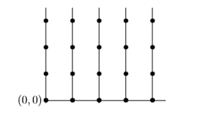
Figure 1. Comb graph: $\mathbb{N}\rhd\mathbb{N}$

A natural coordinate structure is associated to the Comb graph $\mathcal{C}$, as subset of the integer lattice $\mathbb{N}^{d}$. The vertex set is then $E=\mathbb{N}^{d}$ and the root is the origin $x^{(0)}:=(0,\cdots,0)$. Each vertex $x$ is identified to a d-tuple of integers $x\equiv(j_{1},\cdots,j_{d})$. For each $k\in\{1,2,\cdots,d\}$ consider

$$e_{k}:=(0,\cdots,0,1,0,\cdots,0)$$

where $1$ appears at the $k^{th}$-component. Let us set

$$W_{n} = \bigg{\{}x\in L\,:\,d(x,x^{(0)})=n\bigg{\}}$$

$$= \bigg{\{}x=(j_{1},\cdots,j_{d})\in\mathbb{N}^{d}\,:\,\sum_{k=1}^{d}j_{k}=1\bigg{\}}.$$

$$\Lambda_{n}=\bigcup_{k=0}^{n}W_{k},\qquad\Lambda_{[n,m]}=\bigcup_{k=n}^{m}W_{k},\ (n<m).$$

Now for each $x\in W_{n}$, we define its direct successors by

$$S(x):=\bigl{\{}y\in W_{n+1}\,:\,x\sim y\bigr{\}}$$

It is obvious that for every vertex $x$ (distinct of the root $x^{(0)}$) one has $|S(x)|=|N_{x}|-1$. In particular, if $x\in\Delta_{k}$ we get $|S(x)|=2(d-k)+1$. Moreover, the tree structure of the considered graph yields to

(2) $$W_{n+1}=\bigcup_{x\in W_{n}}S(x)\quad\hbox{and}\quad S(x)\cap S(y)=\varnothing,\quad\forall x\neq y.$$

3. Quantum Markov chains on the Comb graph

Let $\mathcal{A},\mathcal{B}$ be two unital C^∗-algebras. A completely positive (CP) identity preserving map $\mathcal{E}:\mathcal{A}\otimes\mathcal{B}\to\mathcal{B}$ is called transition expectation. Note the structure of completely positive maps was clarified [4] and its general formulation in terms of density matrices was carried out in the case of full matrix algebras. Mainly, every CP-map $\mathcal{E}:\mathcal{A}\otimes\mathcal{B}\to\mathcal{B}$ is given by

$$\mathcal{E}(x)=\sum_{j}\mathrm{Tr}_{\mathcal{B}]}\bigl{(}K_{j}^{\ast}xK_{j});\quad x\in\mathcal{A}\otimes\mathcal{B}$$

where $K_{j}\in\mathcal{A}\otimes\mathcal{B}$ and $\mathrm{Tr}_{\mathcal{B}}:\mathcal{A}\otimes\mathcal{B}\to\mathcal{B}$ is the partial trace. In particular, if $K\in\mathcal{A}\otimes\mathcal{B}$ is any density, then

(3) $$\mathcal{E}(x)=\mathrm{Tr}_{\mathcal{B}]}(K^{\ast}xK);\quad x\in\mathcal{A}\otimes\mathcal{B}$$

such that

(4) $$\mathrm{Tr}_{\mathcal{B}]}(K^{\ast}K)=I_{\mathcal{B}}$$

is a (identity preserving) transition expectation. In what follows, any operator $K\in\mathcal{A}\otimes\mathcal{B}$ which satisfies (4) will be called conditional density matrix.

Consider a triplet $\mathcal{C}\subseteq\mathcal{B}\subseteq\mathcal{A}$ of C^∗–algebras. A quasi-conditional expectation [2] is a completely positive identity preserving linear map $E:\mathcal{A}\to\mathcal{B}$ such that $E(ca)=cE(a)$, for all $a\in\mathcal{A}$, $c\in\mathcal{C}.$

To each vertex $x$, we associate an algebra of observable $\mathcal{B}_{x}\equiv\mathcal{B}(\mathcal{H}_{x})$ for some finite dimensional Hilbert space $\mathcal{H}_{x}$. Consider the quasi-local algebra $\mathcal{B}_{L}:=\bigotimes_{x\in L}\mathcal{B}_{x}$ which the inductive limit of the net

$$\mathcal{B}_{\Lambda}:=\bigotimes_{x\in\Lambda}\mathcal{B}_{x}\otimes I_{\Lambda^{c}};\quad\Lambda\subset L,\,|\Lambda|<\infty.$$

Then

$$\mathcal{B}_{L}=\overline{\mathcal{B}_{L,loc}}^{C^{\ast}}$$

where

$$\mathcal{B}_{L,loc}=\bigcup_{\Lambda\subset_{fin}L}\mathcal{B}_{V}.$$

For the sake of simplicity, we will denote

$$\mathcal{B}_{[m,n]}:=\mathcal{B}_{\Lambda_{[m,n]}}.$$

Starting from any quasi-conditional expectation $E_{n}:\mathcal{B}_{[0,n+1]}\to\mathcal{B}_{[0,n]}$ with respect to the triplet $\mathcal{B}_{[0,n-1]}\subseteq\mathcal{B}_{[0,n-1]}\subseteq\mathcal{B}_{[0,n]}$ one can obtain a transition expectation from $\mathcal{B}_{[n,n+1]}$ into $\mathcal{B}_{W_{n}}$ by the mere restriction

$$\mathcal{E}_{[n,n+1]}:=E_{n}\Big{|}_{\mathcal{B}_{[n,n+1]}}.$$

Conversely, every transition expectation $\mathcal{E}_{[n,n+1]}:\mathcal{B}_{[n,n+1]}\to B_{W_{n}}$ is extendable to a quasi-conditional expectation $E_{n}$ with respect to the above triplet in the following way

(5) $$E_{n}:=id_{\mathcal{B}_{n-1]}}\otimes\mathcal{E}_{[n,n+1]}.$$

Definition 3.1.

A state $\varphi$ on $\mathcal{B}_{L}$ is called quantum Markov chain (QMC) with respect to a triplet $\big{(}\rho_{0},\{\mathcal{E}_{[n,n+1]}\},\{h_{n}\}\big{)}$, where $\rho_{0}$ is a state on $\mathcal{B}_{x^{(0)}}$, $\mathcal{E}_{[n,n+1]}:\mathcal{B}_{[n,n+1]}\to\mathcal{B}_{W_{n}}$ is a transition expectation and $\{h_{n}\}\subset\mathcal{B}_{W_{n},+}$ is a sequence of boundary conditions) if

(6) $$\varphi=\lim_{n\to+\infty}\rho_{0}\circ E_{0}\circ E_{1}\circ\cdots\circ E_{n}\circ{\mathbf{h}}_{n+1}$$

where ${\mathbf{h}}_{k}(\cdot)=h_{k}^{1/2}(\cdot)h_{k}^{1/2}$. Here we have used the notation (5).

Thanks to (5), we can immediately verify that, the QMC $\varphi$ is evaluated at $a=a_{0}\otimes a_{1}\otimes\dots\otimes a_{W_{n}}\in\mathcal{B}_{[0,n]}$, $a_{j}\in\mathcal{B}_{W_{j}}$, by

$$\varphi(a)=\lim_{n\to+\infty}\rho_{0}\Bigl{(}\mathcal{E}_{[0,1]}\Bigl{(}a_{W_{0}}\otimes\mathcal{E}_{[1,2]}\Bigl{(}a_{1}\otimes\cdots\otimes\mathcal{E}_{[n,n+1]}\Bigl{(}h^{1/2}_{n+1}a_{n}h^{1/2}_{n+1}\otimes I\Bigr{)}\Bigr{)}\Bigr{)}\Bigr{)}$$

which highlights the quantum Markov chain structure.

We notice that a more general definition of QMC has been formulated in [5, 10].

4. Construction of QMC on $\mathbb{N}^{\rhd d}$

This section is devoted to a construction of quantum Markov chains associated with nearest-neighbors interactions on the algebra $\mathcal{B}_{L}$.

Let $K_{[n,n+1]}\in\mathcal{B}_{[n,n+1]}$ be a conditional density matrix and let $\mathcal{E}_{[n,n+1]}:\mathcal{B}_{[n,n+1]}\to\mathcal{B}_{W_{n}}$ its associated transition expectation given by

(7) $$\mathcal{E}_{[n,n+1]}(a)=\mathrm{Tr}_{\mathcal{B}_{W_{n}}]}\bigl{(}K_{[n,n+1]}^{\ast}aK_{[n,n+1]}\bigr{)}$$

Note that (2) leads to the identity

$$\mathcal{B}_{[n,n+1]}\equiv\bigotimes_{x\in W_{n}}\mathcal{B}_{x\cup S(x)}$$

A transition expectation $\mathcal{E}_{[n,n+1]}:\mathcal{B}_{[n,n+1]}\to\mathcal{B}_{W_{n}}$ is said to be localized if it can be decomposed as follows

(8) $$\mathcal{E}_{[n,n+1]}=\bigotimes_{x\in W_{n}}\mathcal{E}_{x}$$

for some transition expectation $\mathcal{E}_{x}:\mathcal{B}_{\{x\}\cup S(x)}\to\mathcal{B}_{x}$ for each vertex $x\in W_{n}$.

Note that the partial trace $\mathrm{Tr}_{\mathcal{B}_{W_{n}}]}$ is by construction localized

$$\mathrm{Tr}_{\mathcal{B}_{W_{n}}]}=\bigotimes_{x\in W_{n}}\mathrm{Tr}_{\mathcal{B}_{\{x\}\cup S(x)}]}$$

One can see that the localized transition expectation $\mathcal{E}_{[n,n+1]}$ highlights the fine structure of the considered graph. This property played an essential role in the study of phase transitions for quantum Markov chains on the Cayley tree [37].

Definition 4.1.

A conditional density operator $K_{[n,n+1]}\in\mathcal{B}_{[n,n+1]}$ is said to be localized if

(9) $$K_{[n,n+1]}=\bigotimes_{x\in W_{n}}K_{\{x\}\cup S(x)}$$

where $K_{\{x\}\cup S(x)}\in\mathcal{B}_{\{x\}\cup S(x)}$ for every $x\in W_{n}$.

We immediately can prove the following fact.

Lemma 4.2.

If the conditional density matrix $K_{[n,n+1]}=\bigotimes_{x\in W_{n}}K_{\{x\}\cup S(x)}$ is localized then the associated quasi-conditional expectation $\mathcal{E}_{[n,n+1]}$ is localized in the sense of (8) with

(10) $$\mathcal{E}_{x}(\cdot)=\mathrm{Tr}_{\mathcal{B}_{x}}\Bigl{(}K_{\{x\}\cup S(x)}^{\ast}\cdot K_{\{x\}\cup S(x)}\Bigr{)}.$$

for each $x\in W_{n}$.

In the sequel, the pair $\{\rho_{0},h=(h_{n})\}$ denotes a boundary condition such that $\rho_{0}$ is a faithful positive linear functional on the algebra $\mathcal{B}_{(x_{0})}$ and $h_{n}\in\mathcal{B}_{W_{n}}^{+}$ for each $n$.

Let $\varphi^{(\rho_{0},h)}_{n}$ be a linear functional on $\mathcal{B}_{[0,n]}$ given by

(11) $$\varphi^{(\rho_{0},h)}_{n}(a)=\rho_{0}\bigl{(}E_{0}\bigl{(}E_{1}\bigl{(}\cdots\bigl{(}E_{n}\bigl{(}h^{1/2}_{n+1}ah^{1/2}_{n+1}\bigr{)}\bigr{)}\bigr{)}\bigr{)}\bigr{)}.$$

Observe that for each $a\in\mathcal{B}_{[0,n]}$, one has

$$E_{n}\bigl{(}h_{n+1}^{1/2}(a\otimes I)^{\ast}(a\otimes I)h_{n+1}^{1/2}\bigr{)}\geq 0$$

and since the maps $\mathcal{E}_{[j,j+1]}$ are completely positive and the functional $\rho_{0}$ is a positive functional then the functional $\varphi^{(\rho_{0},h)}_{n}$ is positive.

The sequence $\{\varphi^{(\rho_{0},h)}_{n}\}_{n}$ satisfies the compatibility condition if

(12) $$\varphi_{n+1}^{(\rho_{0},h)}\Big{|}_{\mathcal{B}_{[0,n]}}=\varphi^{(\rho_{0},h)}_{n},\quad\ \textrm{for all}\ n.$$

Clearly, the compatibility condition ensures the existence of the weak-limit

$$\lim_{n\to\infty}\varphi^{(\rho_{0},h)}_{n}.$$

Lemma 4.3.

For the same notations as above, if

(13) $$\mathcal{E}_{[n,n+1]}(h_{n+1})=h_{n}\quad;\quad\forall n\in\mathbb{N}$$

then the sequence $\{\varphi^{(\rho_{0},h)}_{n}\}_{n}$ given by (11) satisfies the compatibility condition (12).

Proof.

Let $a\in\mathcal{B}_{\Lambda_{n}}$. Due to $[h_{n+i},a]=0$, ($i=1,2$) we find

$$\varphi_{n+1}^{(\rho_{0},h)}(a) = \rho_{0}\bigl{(}\mathcal{E}_{[0,1]}\bigl{(}\mathcal{E}_{[1,2]}\bigl{(}\cdots\mathcal{E}_{[n,n+1]}\bigl{(}\mathcal{E}_{[n+1,n+2]}\bigl{(}h_{n+2}a\otimes I\bigr{)}\bigr{)}\cdots\bigr{)}\bigr{)}\bigr{)}\bigr{)},$$

$$= \rho_{0}\bigl{(}\mathcal{E}_{[0,1]}\bigl{(}\mathcal{E}_{[1,2]}\bigl{(}\cdots\mathcal{E}_{[n,n+1]}\bigl{(}\mathcal{E}_{[n+1,n+2]}\bigl{(}h_{n+2}\bigr{)}a\otimes I\bigr{)}\cdots\bigr{)}\bigr{)}\bigr{)}\bigr{)},$$

$$= \rho_{0}\bigl{(}\mathcal{E}_{[0,1]}\bigl{(}\mathcal{E}_{[1,2]}\bigl{(}\cdots\mathcal{E}_{[n,n+1]}\bigl{(}h_{n+1}a\otimes I\bigr{)}\cdots I\bigr{)}\cdots\bigr{)}\bigr{)}\bigr{)}\bigr{)},$$

$$= \rho_{0}\bigl{(}\mathcal{E}_{[0,1]}\bigl{(}\mathcal{E}_{[1,2]}\bigl{(}\cdots\mathcal{E}_{[n,n+1]}\bigl{(}h^{1/2}_{n+1}ah^{1/2}_{n+1}\otimes I\bigr{)}\cdots I\bigr{)}\cdots\bigr{)}\bigr{)}\bigr{)}\bigr{)},$$

$$= \varphi_{n}^{(\rho_{0},h)}(a).$$

This completes the proof. ∎

Theorem 4.4.

Let $K_{\{x\}\cup S(x)}\in\mathcal{B}_{\{x\}\cup S(x)}$ be given as above. Assume that the boundary condition $(\rho_{o},h=(h_{u})_{u\in L})$ satisfies the following conditions

(14) $$\rho_{o}(h_{o})=1$$

(15) $$\mathrm{Tr}_{\mathcal{B}_{x}]}\Bigl{(}K_{\{x\}\cup S(x)}^{\ast}I^{(x)}\otimes\bigotimes_{y\in S(x)}h^{(y)}K_{\{x\}\cup S(x)}\Bigr{)}=h^{(x)}$$

then the sequence $\{\varphi^{(\rho_{0},h)}_{n}\}$ satisfies the compatibility condition (12). Moreover, there exists a quantum Markov chain.

Proof.

From Lemma 4.2, the maps $\mathcal{E}_{[n,n+1]}$ are completely positive and localized in the sense of (8). One finds

$$\mathcal{E}_{[n,n+1]}(h_{n+1}) = \mathrm{Tr}_{\mathcal{B}_{W_{n}}]}\bigl{(}K_{[n,n+1]}^{\ast}h_{n}K_{[n,n+1]}\bigr{)},$$

$$= \bigotimes_{x\in W_{n}}\Bigl{(}K_{\{x\}\cup S(x)}^{\ast}I^{(x)}\otimes\bigotimes_{y\in S(x)}h^{(y)}K_{\{x\}\cup S(x)}\Bigr{)},$$

$$= \bigotimes_{x\in W_{n}}h^{(x)},$$

$$= h_{n}.$$

Hence, by virtue of Lemma 4.3, we get the desired assertion, which completes the proof. ∎

5. Quantum Markov chains associated with Ising type models on the Comb graph $\mathbb{N}\rhd_{0}\mathbb{N}$

In this and the forthcoming sections, we restrict ourselves to a semi-infinite Comb graph $\mathbb{N}\rhd_{0}\mathbb{N}$ with distinguished vertex $x^{(0)}=(0,0)$. In what follows, as usually, by $L$ we denote the set of all vertices and $E$ is the set of edges of $\mathbb{N}\rhd_{0}\mathbb{N}$, respectively. A simple coordinate structure is naturally associated to the $\mathbb{N}\rhd_{0}\mathbb{N}$. Each vertex $x$ is identified with a pair of non-negative integers $x\equiv(k,l)$. Here $k$ is the component of $x$ on the horizontal axis and $l$ on the vertical one.

We enumerate elements of $W_{n}$ in the following way

(16) $$x_{W_{n}}^{(0)}=(n,0)\quad\,x_{W_{n}}^{(1)}=(n-1,1)\quad\,\cdots\quad\,x_{W_{n}}^{(n)}=(0,n)$$

and we write

$$\overrightarrow{W}_{n}:=\bigl{\{}x_{W_{n}}^{(0)},x_{W_{n}}^{(1)},\cdots,x_{W_{n}}^{(n)}\bigr{\}}.$$

Accordingly, we distinguish two different types of vertices: ones having two direct successors and others having only one. Define

(17) $$L_{1}=\{x\in L\,:\,|S(x)|=1\}$$

(18) $$L_{2}=\{x\in L\,:\,|S(x)|=2\}=\{x_{W_{n}}^{(0)}\ :\ n\in\mathbb{N}\}$$

here as before, $S(x)$ denotes the direct successors of $x$.

It is clear that $L=L_{1}\cup L_{2}$. For $u\in L_{2}$ one has

$$S(u)=\{u+e_{1},\,u+e_{2}\}$$

whereas, elements of $L_{1}$ have a form $v=(k,l)$ with $l\geq 1$ and

$$S(v)=\{v+e_{2}\}$$

where $e_{1}=(1,0)$ and $e_{2}=(0,1)$.

Denote

(19) $${\bf 1}\!\!{\rm I}^{(u)}=\left(\begin{array}[]{cc}1&0\\ 0&1\\ \end{array}\right),\ \,\ \sigma_{z}^{(u)}=\left(\begin{array}[]{cc}1&0\\ 0&-1\\ \end{array}\right).$$

In what follows, we consider the same $C^{*}$-algebra $\mathcal{B}_{L}$ but with $\mathcal{B}_{u}=M_{2}(\mathbb{C})$ for all $u\in L$.

Let $h^{(u)}=\left(\begin{array}[]{cc}h^{(u)}_{11}&h^{(u)}_{12}\\ h^{(u)}_{21}&h^{(u)}_{22}\\ \end{array}\right)\in M_{2}(\mathbb{C})^{+}$. The family $\{h^{(u)},\,u\in L\}$ is said to be homogeneous (or translation invariant) boundary conditions if $h^{(u)}=h^{(x^{0})}$ for each $u\in L$. We are interested in the resolution of the equations

(20) $$\mathrm{Tr}\left(K_{\{u\}\cup\overrightarrow{S}(u)}^{\ast}{\bf 1}\!\!{\rm I}^{(u)}\otimes h_{S(u)}K_{\{u\}\cup\overrightarrow{S}(u)}\right)=h^{(u)},$$

where

$$\left\{\begin{array}[]{cc}K_{\{u\}\cup S(u)}\in\mathcal{B}_{u}\otimes\mathcal{B}_{u+e_{2}};\quad h_{S(u)}=h^{(u)}\otimes h^{(u+e_{2})}&\hbox{if $u\in L_{1}$;}\\ \\ K_{\{u\}\cup S(u)}\in\mathcal{B}_{u}\otimes\mathcal{B}_{u+e_{1}}\otimes\mathcal{B}_{u+e_{2}};\quad h_{S(u)}=h^{(u)}\otimes h^{(u+e_{1})}\otimes h^{(u+e_{2})}&\hbox{if $u\in L_{2}$.}\\ \end{array}\right.$$

In this paper, we restrict ourselves to the description of translation-invariant solutions of (15). Therefore, we always assume that: $h^{x}=h$ for all $x\in L$, here

$$h=\left(\begin{array}[]{cc}h_{11}&h_{12}\\ h_{21}&h_{22}\\ \end{array}\right).$$

5.1. An Ising model on vertices with degree two

In this subsection, we investigate a concrete Ising type model associated on vertices $v\in L_{1}$ and their successors.

Define

(21) $$\tilde{K}_{<v,v+e_{2}>}=\cos(\beta){\bf 1}\!\!{\rm I}^{(v)}\otimes{\bf 1}\!\!{\rm I}^{(v+e_{2})}-\sin(\beta)\sigma_{z}^{(v)}\otimes\sigma_{z}^{(v+e_{2})}$$

Put

$$K_{\{v\}\cup S(u)}=\tilde{K}_{<v,v+e_{2}>}.$$

Then (20) reduces to

(22) $$\mathrm{Tr}\left(\tilde{K}_{<u,u+e_{2}>}{\bf 1}\!\!{\rm I}^{(u)}\otimes h^{(u+e_{2})}\tilde{K}_{<u,u+e_{2}>}\right)=h^{(u)}$$

One can calculate

$$K_{\{u\}\cup S(u)}{\bf 1}\!\!{\rm I}^{(u)}\otimes h^{(u+e_{2})}K_{\{u\}\cup S(u)}^{\ast}$$

$$=\cos^{(2)}(\beta){\bf 1}\!\!{\rm I}^{(u)}\otimes h^{(u+e_{2})}-\cos(\beta)\sin(\beta)\sigma_{z}^{(u)}\otimes h^{(u+e_{2})}\sigma_{z}^{(u+e_{2})}$$

$$-\cos(\beta)\sin(\beta)\sigma_{z}^{(u)}\otimes\sigma_{z}^{(u+e_{2})}h^{(u+e_{2})}+\sin^{2}(\beta){\bf 1}\!\!{\rm I}^{(u)}\otimes\sigma_{z}h^{(u+e_{2})}\sigma_{z}.$$

Hence, (22) is equivalent to

$$\left\{\begin{array}[]{ll}\left(\frac{h^{(u+e_{2})}_{11}+h^{(u+e_{2})}_{22}}{2}\right)-\sin(2\beta)\left(\frac{h^{(u+e_{2})}_{11}-h^{(u+e_{2})}_{22}}{2}\right)=h^{(u)}_{11};\\ \\ \left(\frac{h^{(u+e_{2})}_{11}+h^{(u+e_{2})}_{22}}{2}\right)+\sin(2\beta)\left(\frac{h^{(u+e_{2})}_{11}-h^{(u+e_{2})}_{22}}{2}\right)=h^{(u)}_{22};\\ \\ h^{(u)}_{12}=h^{(u)}_{21}=0.\end{array}\right.$$

According to the positivity of $h$, a simple calculation leads to the solution

(23) $$h^{(u)}=a{\bf 1}\!\!{\rm I}^{(u)},\quad a>0.$$

5.2. An Ising model on vertices with degree three

In this subsection, we consider another type of Ising model on triples $(v,v+e_{1},v+e_{2})$ for each $v\in L_{2}$.

Define nearest neighbors interactions by

(24) $$K_{<v,(v+e_{i})>}=\exp\{\beta H_{<v,(v+e_{i})>}\},\ \ i=1,2,\ \beta>0,$$

where

(25) $$H_{<v,(v,i)>}=\frac{1}{2}\big{(}{\bf 1}\!\!{\rm I}^{v)}{\bf 1}\!\!{\rm I}^{(v+e_{i})}+\sigma_{z}^{(v)}\sigma_{z}^{(v+e_{i})}\big{)},$$

and the one level nearest neighbours interaction between $v+e_{1}$ and $v+e_{2}$ by

(26) $$L_{>v+e_{1},v+e_{2}<}=\exp\{J\beta H_{>v+e_{1},v+e_{2}<}\},\ \ J>0,$$

where

(27) $$H_{>v+e_{1},v+e_{2}<}=\frac{1}{2}\big{(}{\bf 1}\!\!{\rm I}^{v+e_{1}}{\bf 1}\!\!{\rm I}^{v+e_{2}}+\sigma_{z}^{v+e_{1}}\sigma_{z}^{v+e_{2}}\big{)}.$$

The constant $J>0$ is known in the physics literature as coupling constant.

The defined model is called an Ising model with competing interactions per vertices $(v,(v+e_{1}),(v+e_{2}))$.

One can check that

$$H_{<u,u+e_{i}>}^{m}=H_{<u,u+e_{i}>}=\frac{1}{2}\big{(}{\bf 1}\!\!{\rm I}^{(u)}{\bf 1}\!\!{\rm I}^{(u+e_{i})}+\sigma_{z}^{(u)}\sigma_{z}^{(u+e_{i})}\big{)},$$

$$H_{>u+e_{1},u+e_{2}<}^{m}=H_{>u+e_{1},u+e_{2}<}=\frac{1}{2}\big{(}{\bf 1}\!\!{\rm I}^{(u+e_{1})}{\bf 1}\!\!{\rm I}^{(u+e_{2})}+\sigma_{z}^{(u+e_{1})}\sigma_{z}^{(u+e_{2})}\big{)}.$$

Therefore,

(28) $$K_{<u,u+e_{i}>}=K_{0}{\bf 1}\!\!{\rm I}^{(u)}{\bf 1}\!\!{\rm I}^{(u+e_{i})}+K_{3}\sigma_{z}^{(u)}\sigma_{z}^{(u+e_{i})},$$

(29) $$L_{>u+e_{1},u+e_{2}<}=R_{0}{\bf 1}\!\!{\rm I}^{(u+e_{1})}{\bf 1}\!\!{\rm I}^{(u+e_{3})}+R_{3}\sigma_{z}^{(u+e_{1})}\sigma_{z}^{(u+e_{2})},$$

here

$$K_{0}=\frac{\exp{\beta}+1}{2},\ \ \ K_{3}=\frac{\exp{\beta}-1}{2},$$

$$R_{0}=\frac{\exp{(J\beta)}+1}{2},\ \ \ R_{3}=\frac{\exp{(J\beta)}-1}{2}.$$

For each $u\in L_{2}$, we define

(30) $$K_{\{v\}\cup S(v)}=K_{<v,v+e_{1}>}K_{<v,v+e_{2}>}L_{>v+e_{1},v+e_{2}<}.$$

Hence, (20) reduces to

(31) $$\mathrm{Tr}_{u]}\left(K_{\{v\}\cup S(v)}^{*}{\bf 1}\!\!{\rm I}^{(u)}\otimes h^{(u+e_{1})}\otimes h^{(u+e_{2})}K_{\{v\}\cup S(v)}\right)=h^{(u)}.$$

From (28) and (29), it follows that

(32) $$K_{\{v\}\cup S(v)} = A{\bf 1}\!\!{\rm I}^{(v)}\otimes{\bf 1}\!\!{\rm I}^{(v+e_{1})}\otimes{\bf 1}\!\!{\rm I}^{(v+e_{2})}+B\sigma_{z}^{(v)}\otimes\sigma_{z}^{(v+e_{1})}\otimes{\bf 1}\!\!{\rm I}^{(v+e_{2})}$$

$$+B\sigma_{z}^{(v)}\otimes{\bf 1}\!\!{\rm I}^{(v+e_{1})}\otimes\sigma_{z}^{(v+e_{2})}+C{\bf 1}\!\!{\rm I}^{(v)}\otimes\sigma_{z}^{(v+e_{1})}\otimes\sigma_{z}^{(v+e_{2})},$$

where

(33) $$\left\{\begin{array}[]{ll}A=K_{0}^{2}R_{0}+K_{3}^{2}.R_{3}=\frac{1}{4}[\exp{(J+2)\beta}+\exp{J\beta}+2\exp{\beta}],\\ \\ B=K_{0}K_{3}(R_{0}+R_{3})=\frac{1}{4}\exp{J\beta}[\exp{2\beta}-1],\\ \\ C=K_{0}^{2}R_{3}+K_{3}^{2}R_{0}=\frac{1}{4}[\exp{(J+2)\beta}+\exp{J\beta}-2\exp{\beta}].\\ \end{array}\right.$$

Then

$$K_{\{v\}\cup S(v)}^{\ast}\times[{\bf 1}\!\!{\rm I}^{(v)}\otimes h^{(v+e_{1})}\otimes h^{(v+e_{2})}]\times K_{\{v\}\cup S(v)}$$

$$= \big{[}A^{2}{\bf 1}\!\!{\rm I}\otimes h\otimes h+B^{2}{\bf 1}\!\!{\rm I}\otimes\sigma_{z}h\sigma_{z}\otimes h+B^{2}{\bf 1}\!\!{\rm I}\otimes h\otimes\sigma_{z}h\sigma_{z}+C^{2}{\bf 1}\!\!{\rm I}\otimes\sigma_{z}h\sigma_{z}\otimes\sigma_{z}h\sigma_{z}\big{]}$$

$$+ \big{[}AC{\bf 1}\!\!{\rm I}\otimes h\sigma_{z}\otimes h\sigma_{z}+AC{\bf 1}\!\!{\rm I}\otimes\sigma_{z}h\otimes\sigma_{z}h+B^{2}{\bf 1}\!\!{\rm I}\otimes\sigma_{z}h\otimes h\sigma_{z}+B^{2}{\bf 1}\!\!{\rm I}\otimes h\sigma_{z}\otimes\sigma_{z}h\big{]}$$

$$+ \big{[}AB\sigma_{z}\otimes h\sigma_{z}\otimes h+AB\sigma_{z}\otimes h\otimes h\sigma_{z}+AB\sigma_{z}\otimes h\otimes\sigma_{z}h+AB\sigma_{z}\otimes\sigma_{z}h\otimes h\big{]}$$

$$+ \big{[}BC\sigma_{z}\otimes\sigma_{z}h\sigma_{z}\otimes h\sigma_{z}+BC\sigma_{z}\otimes h\sigma_{z}\otimes\sigma_{z}h\sigma_{z}+BC\sigma_{z}\otimes\sigma_{z}h\sigma_{z}\otimes\sigma_{z}h+BC\sigma_{z}\otimes\sigma_{z}h\otimes\sigma_{z}h\sigma_{z}\big{]}.$$

Therefore, due to the last equality, we rewrite (31) as follows

(34) $$h^{(v)} = \mathrm{Tr}_{x]}K_{\{v\}\cup S(v)}^{*}\left({\bf 1}\!\!{\rm I}^{(v)}\otimes h\otimes h\right)K_{\{v\}\cup S(v)}$$

$$= \left(\tau_{1}{\mathrm{Tr}(h)}^{2}+\tau_{2}{\mathrm{Tr}(\sigma_{z}h)}^{2}\right){\bf 1}\!\!{\rm I}^{(v)}+\tau_{3}\mathrm{Tr}(h)\mathrm{Tr}(\sigma_{z}h)\sigma_{z}^{(v)},$$

where $\theta=\exp(2\beta)>0$ and

(35) $$\left\{\begin{array}[]{ll}\tau_{1}:=A^{2}+2B^{2}+C^{2}=\frac{1}{4}[\theta^{J}(\theta^{2}+1)+2\theta],\\ \\ \tau_{2}:=2(AC+B^{2})=\frac{1}{4}[\theta^{J}(\theta^{2}+1)-2\theta],\\ \\ \tau_{3}:=4B(A+C)=\frac{1}{2}\theta^{J}(\theta^{2}-1).\end{array}\right.$$

From

$$\mathrm{Tr}(h)=\frac{h_{11}+h_{22}}{2}\quad;\quad\mathrm{Tr}(\sigma_{z}h)=\frac{h_{11}-h_{22}}{2}$$

the equation (34) reduces to

(36) $$\left\{\begin{array}[]{lll}\mathrm{Tr}(h)=\tau_{1}\mathrm{Tr}(h)^{2}+\tau_{2}\mathrm{Tr}(\sigma_{z}h)^{2},\\ \\ \mathrm{Tr}(\sigma_{z}h)=\tau_{3}\mathrm{Tr}(h)\mathrm{Tr}(\sigma_{z}h),\\ \\ h_{21}=0,\quad h_{12}=0.\\ \end{array}\right.$$

Since, we are interested in transition-invariant solutions, it is convenient to find those one with $h_{1,1}=h_{2,2}$. So, (36) is reduced to

$$h_{11}=h_{22}=\frac{1}{\tau_{1}}.$$

Hence,

(37) $$h^{(u)}=\frac{1}{\tau_{1}}{\bf 1}\!\!{\rm I}^{(u)};\quad\forall u\in L_{2}.$$

Now we are ready to formulate a main result of this section.

Theorem 5.1.

For the Ising (ZZ) coupling model (21) and the Ising model with competing interactions (24), (26),  $\beta>0,J>0$ on the Comb graph $\mathbb{N}\rhd_{0}\mathbb{N}$, there exists a quantum Markov chain $\varphi$ with homogeneous boundaries. Moreover, it can be written on the local algebra $\mathcal{B}_{L,loc}$ by:

(38) $$\varphi(a)=\alpha^{n}\mathrm{Tr}\bigg{(}a\prod_{i=0}^{n-1}K_{[i,i+1]}K_{[i,i+1]}^{*}\bigg{)},\ \ \forall a\in B_{[0,n]}.$$

We notice that the QMC $\varphi$ is called disordered phase of the Ising model.

Proof.

According to the Ising type models considered in the subsection 5.1 and the subsection 5.2, the equation (20) admits a unique translation-invariant solution

(39) $$h^{(u)}_{\alpha}=\left(\begin{array}[]{cc}\alpha&0\\ 0&\alpha\\ \end{array}\right)$$

where $\alpha=\frac{1}{\tau_{1}}$. The initial functional $\rho_{0}$ can be chosen of the form

$$\rho_{0}(a)=\tau_{1}\mathrm{Tr}(a)$$

so that $\rho_{0}(h^{x^{(0)}})=\mathrm{Tr}(\omega_{0}h^{x^{(0)}})=1$, where $\omega_{0}=\tau_{1}{\bf 1}\!\!{\rm I}^{x^{(0)}}$
Let $n\in\mathbb{N},a\in B_{[0,n]}$, according (39) and from Lemma 4.3, one finds

$$\varphi(a) = \varphi_{n}^{(\rho_{0},h)}(a)$$

$$= \rho_{0}\Bigl{(}\mathcal{E}_{[0,1]}\Bigl{(}a_{W_{0}}\otimes\mathcal{E}_{[1,2]}\Bigl{(}a_{1}\otimes\cdots\otimes\mathcal{E}_{[n-1,n+1]}\Bigl{(}h_{n}a\Bigr{)}\Bigr{)}\Bigr{)}\Bigr{)}$$

$$= \mathrm{Tr}\bigl{(}\omega_{0}\mathrm{Tr}_{\mathcal{B}_{W_{0}]}}\Bigl{(}K_{[0,1]}^{*}\mathrm{Tr}_{\mathcal{B}_{W_{1}]}}\Bigl{(}K_{[1,2]}^{*}\cdots\otimes\mathrm{Tr}_{\mathcal{B}_{W_{n-1}]}}\Bigl{(}K_{[n-1,n]}^{*}h_{n}aK_{[n-1,n]}\Bigr{)}\cdots K_{[1,2]}\Bigr{)}K_{[0,1]}\Bigr{)}\Bigr{)}$$

$$= \mathrm{Tr}\bigg{(}\omega_{0}h_{n}\bigg{(}\prod_{m=0}^{n-1}K_{[m,m+1]}^{*}aK_{[m,m+1]}\bigg{)}\bigg{)}$$

$$= \alpha^{|W_{n}|-1}\mathrm{Tr}\bigg{(}a\prod_{m=0}^{n-1}K_{[m,m+1]}K_{[m,m+1]}^{*}\bigg{)}$$

$$= \alpha^{n}\mathrm{Tr}\bigg{(}a\prod_{i=0}^{n-1}K_{[i,i+1]}K_{[i,i+1]}^{*}\bigg{)}.$$

This completes the proof. ∎

6. Clustering property

The Comb graph $\mathbb{N}\rhd_{0}\mathbb{N}=(V,E)$ is invariant under the action of the semi-group $\mathcal{G}^{+}$ of translations of the form

(40) $$J_{n}:u=(k,l)\in\mathbb{N}\times\mathbb{N}\mapsto u+ne_{1}=(k+n,l).$$

For each $g=(n,0)\in L_{2}$ we denote

$$\tau_{g}(u):=J_{n}(u).$$

In these notations, we have $\mathcal{G}^{+}:=\{\tau_{g}\ :\ g\in L_{3}\}$.

Lemma 6.1.

Assume that $n_{0}\in\mathbb{N}$. Let $a\in\mathcal{B}_{[0,n_{0}]}$ and $b\in\mathcal{B}_{x^{(0)}}$. Then

(41) $$\lim_{n\to+\infty}\varphi(aJ_{n}(b))=\varphi(a)\varphi(b),$$

where $J_{n}(b)=b^{(x_{W_{n}}^{(0)})}$.

Proof.

For large enough $n$, one gets $ab_{n}=a\otimes b_{n}$, $n>n_{0}$. So,

$$\varphi(a\otimes b_{n}) = \varphi_{n}^{(\rho_{0},h_{\alpha})}(a\otimes b_{n})$$

$$= \rho_{0}\circ\mathcal{E}_{[0,1]}\circ\cdots\circ\mathcal{E}_{[n_{0},n_{0}+1]}(a\otimes\mathcal{E}_{[n_{0}+1,n_{0}+2]}({\bf 1}\!\!{\rm I}_{W_{n_{0}+1}}\otimes\cdots$$

$$\otimes\mathcal{E}_{[n-1,n]}\circ\hat{\mathcal{E}}_{[n,n+1]}(b_{n}\otimes{\bf 1}\!\!{\rm I}_{W_{n+1}}).$$

Here, the boundary condition is taken, as before, $h^{(u)}=h_{\alpha}=\alpha{\bf 1}\!\!{\rm I}$ is a common fixed points of the systems (22) and (31) and the initial state $\rho(\cdot)=\mathrm{Tr}(\omega_{0}\,\cdot),\,\omega_{0}=\frac{1}{\alpha}{\bf 1}\!\!{\rm I}$ with $\alpha=\frac{4}{\theta^{J}(\theta^{2}+1)+2\theta}$.

Then, one finds

$$\hat{\mathcal{E}}_{[n,n+1]}(b_{n}\otimes{\bf 1}\!\!{\rm I}_{W_{n+1}})=\mathrm{Tr}_{n]}\left(K_{[n,n+1]}^{\ast}\mathbf{h}_{n+1}^{1/2}(b\otimes{\bf 1}\!\!{\rm I}_{W_{n+1}})\mathbf{h}_{n+1}^{1/2}K_{[n,n+1]}\right)$$

$$= \bigotimes_{u\in W_{n}}\mathrm{Tr}_{u]}\left(K_{\{u\}\cup S(u)}^{\ast}\bigotimes_{v\in S(u)}(h^{(v)})^{1/2}(b\otimes{\bf 1}\!\!{\rm I}_{W_{n+1}})\bigotimes_{v\in S(u)}(h^{(v)})^{1/2}K_{[n,n+1]}\right)$$

$$= \mathrm{Tr}_{x_{W_{n}}^{(0)}]}\left(K_{\{x_{W_{n}}^{(0)}\}\cup S(x_{W_{n}}^{(0)})}^{\ast}b^{(x_{W_{n}}^{(0)})}\otimes h_{S(x_{W_{n}}^{(0)})}K_{\{x_{W_{n}}^{(0)}\}\cup S(x_{W_{n}}^{(0)})}\right)\otimes$$

$$\bigotimes_{u\in W_{n}\setminus\{x_{W_{n}}^{(0)}\}}\mathrm{Tr}_{u]}\left(K_{\{u\}\cup S(u)}^{\ast}\bigotimes_{v\in S(u)}h^{(v)}K_{[n,n+1]}\right).$$

By (15)

$$\mathrm{Tr}_{u]}\left(K_{\{u\}\cup S(u)}\bigotimes_{v\in S(u)}h^{(v)}K_{[n,n+1]}^{\ast}\right)=h^{(u)}$$

and

$$\mathrm{Tr}_{x_{W_{n}}^{(0)}]}\left(K_{\{x_{W_{n}}^{(0)}\}\cup S(x_{W_{n}}^{(0)})}^{\ast}b^{(x_{W_{n}}^{(0)})}\left({\bf 1}\!\!{\rm I}^{(x_{W_{n}}^{(0)})}\otimes h_{S(x_{W_{n}}^{(0)})}\right)K_{\{x_{W_{n}}^{(0)}\}\cup S(x_{W_{n}}^{(0)})}\right)\\$$

(42) $$=\alpha^{2}\left[(A^{2}+C^{2})b^{(x_{W_{n}}^{(0)})}+2B^{2}\sigma_{z}b^{(x_{W_{n}}^{(0)})}\sigma_{z}\right].$$

Then

$$\mathcal{E}_{[n-1,n]}({\bf 1}\!\!{\rm I}_{W_{n-1}}\otimes\hat{\mathcal{E}}(b^{(x_{W_{n}}^{(0)})}\otimes{\bf 1}\!\!{\rm I}))=\alpha^{2}(A^{2}+C^{2})\mathcal{E}_{[n-1,n]}\left({\bf 1}\!\!{\rm I}_{W_{n-1}}\otimes b^{(x_{W_{n}}^{(0)})}\otimes\bigotimes_{u\in W_{n}\setminus\{x_{W_{n}}^{(0)}\}}h^{(u)}\right)$$

$$+2\alpha^{2}B^{2}\mathcal{E}_{[n-1,n]}\left({\bf 1}\!\!{\rm I}_{W_{n-1}}\otimes\sigma_{z}b^{(x_{W_{n}}^{(0)})}\sigma_{z}\otimes\bigotimes_{u\in W_{n}\setminus\{x_{W_{n}}^{(0)}\}}h^{(u)}\right).$$

A small calculation leads to

$$\mathrm{Tr}_{x_{W_{n-1}}^{(0)}]}\left(K_{\{x_{W_{n-1}}^{(0)}\}\cup S(x_{W_{n-1}}^{(0)})}{\bf 1}\!\!{\rm I}^{(x_{W_{n-1}}^{(0)})}\otimes b^{(x_{W_{n-1}}^{(0)}+e_{1})}\otimes h^{(x_{W_{n-1}}^{(0)}+e_{2})}K_{\{x_{W_{n-1}}^{(0)}\}\cup S(x_{W_{n-1}}^{(0)})}^{*}\right)$$

$$=\alpha\left((A^{2}+2B+C^{2})\mathrm{Tr}(b){\bf 1}\!\!{\rm I}^{x_{W_{n-1}}^{(0)}}+2B(A+C)\mathrm{Tr}(\sigma_{z}b)\sigma_{z}^{x_{W_{n-1}}^{(0)}}\right)$$

$$=\mathrm{Tr}_{x_{W_{n-1}}^{(0)}]}\left(K_{\{x_{W_{n-1}}^{(0)}\}\cup S(x_{W_{n-1}}^{(0)})}{\bf 1}\!\!{\rm I}^{(x_{W_{n-1}}^{(0)})}\otimes(\sigma_{z}b\sigma_{z})^{(x_{W_{n-1}}^{(0)}+e_{1})}\otimes h^{(x_{W_{n-1}}^{(0)}+e_{2})}K_{\{x_{W_{n-1}}^{(0)}\}\cup S(x_{W_{n-1}}^{(0)})}^{*}\right).$$

This implies

$$\mathcal{E}_{[n-1,n]}({\bf 1}\!\!{\rm I}_{W_{n-1}}\otimes\hat{\mathcal{E}}(b^{(x_{W_{n}}^{(0)})}\otimes{\bf 1}\!\!{\rm I}))=\mathrm{Tr}(b)h_{n-1}+\mathrm{Tr}(\sigma_{z}b)(\frac{\tau_{3}}{4\tau_{1}})\sigma_{z}^{x_{W_{n-1}}^{(0)}}h_{n-1}.$$

On the other hand, using (42) one gets

$$\varphi(b^{(o)})=\rho_{0}(\mathcal{E}_{[0,1]}(b^{(o)}\otimes h_{1}))=\mathrm{Tr}(b)$$

Since for each $k\in\mathbb{N}$ we obtain

$$\mathrm{Tr}_{x_{W_{k}}^{(0)}]}\left(K_{\{x_{W_{k}}^{(0)}\}\cup S(x_{W_{k}}^{(0)})}{\bf 1}\!\!{\rm I}^{(x_{W_{k}}^{(0)})}\otimes\sigma_{z}^{(x_{W_{k}}^{(0)}+e_{1})}\otimes h^{(x_{W_{k}}^{(0)}+e_{2})}K_{\{x_{W_{k}}^{(0)}\}\cup S(x_{W_{k}}^{(0)})}^{*}\right)$$

$$=\alpha(A+B)C\sigma_{z}^{(x_{W_{k}}^{(0)})}=\frac{\tau_{3}}{4\tau_{1}}\sigma_{z}^{(x_{W_{k}}^{(0)})}.$$

and taking into account (15), a simple iteration leads to

$$\mathcal{E}_{[k,k+1]}({\bf 1}\!\!{\rm I}\otimes\cdots\mathcal{E}_{[n-1,n]}({\bf 1}\!\!{\rm I}\otimes\hat{\mathcal{E}}_{[n,n+1]}(b^{x_{W_{n}}^{(1)}})=\varphi(b)h_{k}+\mathrm{Tr}(\sigma_{z}b)\left(\frac{\tau_{3}}{4\tau_{1}}\right)^{n-k}(\sigma_{z}^{(x_{W_{k}}^{(1)})}\otimes{\bf 1}\!\!{\rm I}_{W_{k}\setminus\{x_{W_{k}}^{(1)}\}})h_{k}.$$

In particular, by taking $k=n_{0}+1,n_{0}+2$, one gets

$$\varphi_{n}(aJ_{n}(b))=\varphi(b)\rho_{0}(\mathcal{E}_{[0,1]}(a_{W_{0}}\otimes\mathcal{E}_{[1,2]}(a_{W_{1}}\cdots\mathcal{E}_{[n_{0}-1,n_{0}]}(a_{W_{n_{0}-1}}\otimes\mathcal{E}_{[n_{0},n_{0}+1]}(a_{\Lambda}\otimes h_{n_{0}+1}))))$$

$$+\mathrm{Tr}(\sigma_{z}b)\left(\frac{\tau_{3}}{4\tau_{1}}\right)^{n-n_{0}-2}\rho_{0}(\mathcal{E}_{[0,1]}(a_{W_{0}}\otimes\mathcal{E}_{[1,2]}(a_{W_{1}}\cdots\mathcal{E}_{[n_{0},n_{0}+1]}(a_{\Lambda}\otimes\mathcal{E}_{[n_{0}+1,n_{0}]}(\sigma_{z}^{(x_{W_{n_{0}+1}})}\otimes h_{n_{0}+2})))).$$

Thus

(43) $$\varphi_{n}(aJ_{n}(b))=\varphi(b)\varphi_{n_{0}}(a)+\mathrm{Tr}(\sigma_{z}b)\left(\frac{\tau_{3}}{4\tau_{1}}\right)^{n-n_{0}-2}\varphi_{n_{0}+1}(a\otimes\sigma_{z}^{(x_{W_{n_{0}+1}})}).$$

From (35) it follows that

$$\frac{\tau_{3}}{4\tau_{1}}=\frac{\theta^{J}(\theta^{2}-1)}{2(\theta^{J}(\theta^{2}+1)+2\theta)}\in[0,\frac{1}{2}];\quad\theta=\exp(2\beta)>1,J>0.$$

Now taking the limit $n\to+\infty$ in (43) we arrive at (41). ∎

The main result of this section is the following.

Theorem 6.2.

Let $\varphi$ be a QMC associated with the Ising with (ZZ) coupling model on the comb graph $\mathbb{N}\rhd_{0}\mathbb{N}$. Then

(44) $$\lim_{|g|\to+\infty}\varphi(a\tau_{g}(b))=\varphi(a)\varphi(b)$$

for all $a,b\in\mathcal{B}$.

Proof.

Let $a,b\in\mathcal{B}_{L,loc}$. There exist $n,0,m_{0}\in\mathbb{N}$ such that $a=a_{n_{0}}\in\mathcal{B}_{[0,n_{0}]}$ and $b=b_{m_{0}}\in\mathcal{B}_{[0,m_{0}]}$. Without lost of generality, we may assume that $b$ is localized in the following form

$$b=\bigotimes_{u\in[0,m_{0}]}b_{u}=\bigotimes_{k=0}^{m_{0}}b_{W_{k}};\quad b_{W_{k}}=\bigotimes_{u\in W_{k}}b_{u}\in\mathcal{B}_{W_{k}}$$

One can see that

$$J_{n}(b)=\bigotimes_{u\in[0,m_{0}]}b_{u}^{(u+ne_{1})}=\bigotimes_{v\in[n,n+m_{0}]}\tilde{b}_{v}\in\mathcal{B}_{[n,n+m_{0}]}$$

where

$$\tilde{b}_{v}=\left\{\begin{array}[]{ll}b_{v-ne_{1}},&\hbox{if $v-ne_{1}\in\Lambda_{m_{0}}$;}\\ 1,&\hbox{otherwise.}\end{array}\right.$$

Define

(45) $$F_{J_{n}(W_{k})}(a):=\bigotimes_{v\in J_{n}(W_{k})}\mathrm{Tr}_{v]}\left(K_{\{v\}\cup S(v)}aK^{*}_{\{v\}\cup S(v)}\right);\quad a\in\mathcal{B}_{[k,k+1]}$$

Taking into account (15), one finds

$$\hat{\mathcal{E}}_{[n+m_{0},n+m_{0}+1]}(\tilde{b}_{W_{n+m_{0}}})))=\left(\bigotimes_{v\in J_{n}(W_{m_{0}})}\mathrm{Tr}_{v]}\left(K_{\{v\}\cup S(v)}b_{v}h_{S(v)}K^{*}_{\{v\}\cup S(v)}\right)\right)\otimes\left(\bigotimes_{v\in W_{n+m_{0}}\setminus J_{n}(W_{m_{0}})}h_{v}\right)$$

$$=\alpha^{|W_{m_{0}+1}|}F_{J_{n}(W_{m_{0}})}(\tilde{b}_{J_{n}(W_{m_{0}})})\otimes\left(\bigotimes_{v\in W_{n+m_{0}}\setminus J_{n}(W_{m_{0}})}h_{v}\right).$$

According to the structure of the comb graph $\mathbb{N}\rhd_{0}\mathbb{N}$ one has

$$J_{n}(W_{k+1})=\bigcup_{v\in J_{n}(W_{k})}S(v).$$

Then

$${\mathcal{E}}_{[n+m_{0}-1,n+m_{0}]}(\tilde{b}_{W_{n+m_{0}-1}}\otimes\hat{\mathcal{E}}_{[n+m_{0},n+m_{0}+1]}(\tilde{b}_{W_{n+m_{0}}}))))=$$

$$=\alpha^{|W_{m_{0}+1}|}\bigotimes_{u\in J_{n}(W_{m_{0}-1})}\mathrm{Tr}_{u]}\left(K_{\{u\}\cup S(u)}\tilde{b}_{u}\otimes F_{J_{n}(W_{m_{0}})}(\tilde{b}_{J_{n}(W_{m_{0}})})K_{\{u\}\cup S(u)}\right)$$

$$\otimes\bigotimes_{w\in W_{n+m_{0}-1}\setminus J_{n}(W_{m_{0}-1})}h_{w},$$

$$=\alpha^{|W_{m_{0}+1}|}F_{J_{n}(W_{m_{0}-1})}\left(\tilde{b}_{J_{n}(W_{m_{0}-1})}\otimes F_{J_{n}(W_{m_{0}})}(\tilde{b}_{J_{n}(W_{m_{0}})})\right)\otimes\bigotimes_{w\in W_{n+m_{0}-1}\setminus J_{n}(W_{m_{0}-1})}h_{w}.$$

An iteration leads to

$$\mathcal{E}_{[n,n+1]}(\tilde{b}_{W_{n}}\otimes\cdots\mathcal{E}_{[n+m_{0}-1,n+m_{0}]}(\tilde{b}_{W_{n+m_{0}-1}}\otimes\hat{\mathcal{E}}_{[n+m_{0},n+m_{0}]}(\tilde{b}_{n+m_{0}})))$$

$$=\alpha^{|W_{m_{0}+1}|}F_{J_{n}(W_{0})}\left(\tilde{b}_{J_{n}(W_{0})}\otimes\cdots F_{J_{n}(W_{m_{0}-1})}\left(\tilde{b}_{J_{n}(W_{m_{0}-1})}\otimes F_{J_{n}(W_{m_{0}})}(\tilde{b}_{J_{n}(W_{m_{0}})})\right)\right)\otimes\bigotimes_{w\in W_{n}\setminus J_{n}(W_{0})}h_{w}.$$

Since $J_{n}(W_{0})=\{x_{W_{n}}^{(0)}\}$ and $h_{w}=\alpha{\bf 1}\!\!{\rm I}$ for each $w$ then

$$\mathcal{E}_{[n,n+1]}(\tilde{b}_{W_{n}}\otimes\cdots\mathcal{E}_{[n+m_{0}-1,n+m_{0}]}(\tilde{b}_{W_{n+m_{0}-1}}\otimes\hat{\mathcal{E}}_{[n+m_{0},n+m_{0}]}(\tilde{b}_{n+m_{0}})))$$

$$=\alpha^{|W_{m_{0}+1}|+|W_{n}|-1}F_{x_{W_{n}}^{(0)}}\left(\tilde{b}_{J_{n}(W_{0})}\otimes\cdots F_{J_{n}(W_{m_{0}-1})}\left(\tilde{b}_{J_{n}(W_{m_{0}-1})}\otimes F_{J_{n}(W_{m_{0}})}(\tilde{b}_{J_{n}(W_{m_{0}})})\right)\right)\otimes{\bf 1}\!\!{\rm I}_{W_{n}\setminus\{x_{W_{n}}^{(0)}\}},$$

$$=b_{n}\otimes h_{n+1}$$

where

$$g_{n}:=\alpha^{|m_{0}|}F_{x_{W_{n}}^{(0)}}\left(\tilde{b}_{J_{n}(W_{0})}\otimes\cdots F_{J_{n}(W_{m_{0}-1})}\left(\tilde{b}_{J_{n}(W_{m_{0}-1})}\otimes F_{J_{n}(W_{m_{0}})}(\tilde{b}_{J_{n}(W_{m_{0}})})\right)\right)\in\mathcal{B}_{x_{W_{n}}^{(0)}}.$$

One can easily check that $b_{n}=\alpha^{|m_{0}|}J_{n}(b)$ with

$$g=F_{W_{0}}\left(b_{W_{0}}\otimes\cdots F_{W_{m_{0}-1}}\left(b_{W_{m_{0}-1}}\otimes F_{W_{m_{0}}}(b_{W_{m_{0}}})\right)\right)\in\mathcal{B}_{W_{0}}.$$

Then

$$\varphi(a_{n_{0}}\otimes J_{n}(b_{m_{0}})=\rho_{0}(\mathcal{E}_{[0,1]}(a_{W_{0}}\cdots\mathcal{E}_{[n_{0},n_{0}+1]}(a_{W_{n_{0}}}\otimes\mathcal{E}_{[n_{0},n_{0}+1]}({\bf 1}\!\!{\rm I}_{W_{n_{0}+1}}\otimes\cdots$$

$$\mathcal{E}_{[n,n+1]}(\tilde{b}_{W_{n}}\otimes\cdots\mathcal{E}_{[n+m_{0}-1,n+m_{0}]}(\tilde{b}_{W_{n+m_{0}-1}}\otimes\hat{\mathcal{E}}_{[n+m_{0},n+m_{0}]}(\tilde{b}_{n+m_{0}})))))))$$

$$=\rho_{0}(\mathcal{E}_{[0,1]}(a_{W_{0}}\cdots\mathcal{E}_{[n_{0},n_{0}+1]}(a_{W_{n_{0}}}\otimes\mathcal{E}_{[n_{0},n_{0}+1]}({\bf 1}\!\!{\rm I}_{W_{n_{0}+1}}\otimes\cdots\mathcal{E}_{[n,n+1]}(g_{n}\otimes h_{n+1})))))$$

$$=\alpha^{|m_{0}|}\varphi_{n}(a_{n_{0}}J_{n}(g))$$

By Lemma 6.1, one finds

$$\lim_{n\to+\infty}\varphi_{n}(a_{n_{0}}J_{n}(g))=\varphi(a_{n_{0}})\varphi(g).$$

Due to $F_{W_{k}}=\mathcal{E}_{[k,k+1]}$ for $0\leq k\leq m_{0}$, we obtain

$$\alpha^{|m_{0}|}\varphi(g)=\varphi(b_{m_{0}}).$$

Therefore,

$$\lim_{n\to+\infty}\varphi(a_{n_{0}}J_{n}(b_{m_{0}}))=\varphi(a_{n_{0}})\varphi(b_{m_{0}})$$

which completes the proof. ∎

References

• [1] L. Accardi, “On the noncommutative Markov property,” Funct. Anal. Appl., 9, 1–8 (1975).
• [2] L. Accardi and C. Cecchini, “Conditional expectations in von Neumann algebras and a Theorem of Takesaki,” J. Funct. Anal. 45, 245–273 (1982).
• [3] L. Accardi, and A. Frigerio, “Markovian cocycles,” Proc. Royal Irish Acad. 83A, 251–263 (1983).
• [4] L. Accardi, “Topics on quantum probability,” Physics reports 77(3), 169-192 (1981).
• [5] L. Accardi, F. Fidaleo and F. Mukhamedov, “Markov states and chains on the CAR algebra,” Inf. Dim. Analysis, Quantum Probab. Related Topics 10, 165–183 (2007).
• [6] L. Accardi, F. Mukhamedov and M. Saburov, “On Quantum Markov Chains on Cayley tree I: uniqueness of the associated chain with $XY$-model on the Cayley tree of order two,” Inf. Dim. Analysis, Quantum Probab. Related Topics 14, 443–463 (2011).
• [7] L. Accardi, F. Mukhamedov and M. Saburov, “On Quantum Markov Chains on Cayley tree II: Phase transitions for the associated chain with $XY$-model on the Cayley tree of order three,” Ann. Henri Poincare 12, 1109–1144 (2011).
• [8] L. Accardi, F. Mukhamedov and M. Saburov, “On Quantum Markov Chains on Cayley tree III: Ising model,” J. Stat. Phys. 157, 303–329 (2014).
• [9] L. Accardi, H. Ohno, and F. Mukhamedov, “Quantum Markov fields on graphs,” Inf. Dim. Analysis, Quantum Probab. Related Topics 13, 165–189 (2010).
• [10] L. Accardi, A. Souissi and S. El Gheteb, “Quantum Markov chains: a unification approach,” Inf. Dim. Analysis, Quantum Probab. Related Topics 23, 2050016 (2020).
• [11] L. Accardi and G.S. Watson , Quantum random walks, in book: L. Accardi, W. von Waldenfels (eds) Quantum Probability and Applications IV, Proc. of the year of Quantum Probability, Univ. of Rome Tor Vergata, Italy, 1987, LNM, 1396, 73–88 (1987).
• [12] L. Affleck, E. Kennedy, E.H. Lieb and H. Tasaki, “Valence bond ground states in isortopic quantum antiferromagnets,” Commun. Math. Phys. 115, 477–528 (1988).
• [13] S. Attal, F. Petruccione, C. Sabot and I. Sinayskiy, “Open Quantum Random Walks.” J. Stat. Phys. 147, 832–852 (2012).
• [14] H. Araki and D.A. Evans, “A $C^{*}$-algebra approach to phase transition in the two-dimensional Ising model,” Commun. Math. Phys. 91, 489–503 (1983).
• [15] Baxter R. J. Exactly Solved Models in Statistical Mechanics, (Academic Press, London-New York 1982)
• [16] R. Carbone and Y. Pautrat, “Open quantum random walks: reducibility, period, ergodic properties,” Ann. Henri Poincaré 17, 99–135 (2016).
• [17] J.I. Cirac and F. Verstraete, “Renormalization and tensor product states in spin chains and lattices,” J. Phys. A. Math. Theor. 42 (2009), 504004.
• [18] A. Dhahri, Ch.K. Ko and H.J. Yoo, “Quantum Markov Chains Associated with Open Quantum Random Walks,” J. Stat. Phys. 176, 1272–1295 (2019).
• [19] A. Dhahri and F. Mukhamedov, “Open quantum random walks, quantum Markov chains and recurrence,” Rev. Math. Phys. 31, 1950020 (2019)
• [20] A. Dhahri and F. Mukhamedov, “Open quantum random walk and quantum Markov chains,” Funct. Anal. Appl. 53, 137–142 (2019).
• [21] M. Fannes, B. Nachtergaele and R.F. Werner, “Ground states of VBS models on Cayley trees,” J. Stat. Phys. 66, 939–973 (1992)
• [22] M. Fannes, B. Nachtergaele and R.F. Werner, “Finitely correlated states on quantum spin chains,” Commun. Math. Phys. 144, 443–490 (1992).
• [23] Y. Feng, N. Yu and M. Ying, “Model checking quantum Markov chains”, J. Computer Sys. Sci. 79, 1181–-1198 (2013).
• [24] S. Gudder, “Quantum Markov chains,” J. Math. Phys. 49, 072105 (2008).
• [25] J. Kempe, “Quantum random walks—an introductory overview,” Contemporary Physics, 44, 307–327 (2003).
• [26] N. Konno and H.J. Yoo, “Limit theorems for open quantum random walks,” J. Stat. Phys. 150, 299–319 (2013).
• [27] H.A. Kramers and G.H. Wannier, “Statistics of the two-dimensional ferromagnet. Part II,” Phys. Rev. 60 263 (1941).
• [28] C.R. Laumann, S.A. Parameswaran and S.L. Sondhi, “AKLT models with quantum spin glass ground states,” Phys Rev B 81, 174204 (2010).
• [29] F. Mukhamedov, A. Barhoumi and A. Souissi, “Phase transitions for quantum Markov chains associated with Ising type models on a Cayley tree,” J. Stat. Phys. 163, 544–567 (2016).
• [30] F. Mukhamedov, A. Barhoumi and A. Souissi, “On an algebraic property of the disordered phase of the Ising model with competing interactions on a Cayley tree,” Math. Phys. Anal. Geom. 19, 21 (2016).
• [31] F. Mukhamedov, A. Barhoumi and A. Souissi, and S. El Gheteb, “A quantum Markov chain approach to phase transitions for quantum Ising model with competing XY-interactions on a Cayley tree,” J. Math. Phys. 61, 093505 (2020).
• [32] F. Mukhamedov and S. El Gheteb, “Uniqueness of quantum Markov chain associated with XY-Ising model on the Cayley tree of order two,” Open Sys. & Infor. Dyn. 24, 175010 (2017).
• [33] F. Mukhamedov and S. El Gheteb, “Clustering property of Quantum Markov Chain associated to XY-model with competing Ising interactions on the Cayley tree of order two,” Math. Phys. Anal. Geom. 22, 10 (2019).
• [34] F. Mukhamedov and S. El Gheteb, “Factors generated by $XY$-model with competing Ising interactions on the Cayley tree,” Ann. Henri Poincare 21, 241–253 (2020).
• [35] F. Mukhamedov and U. Rozikov, “ On Gibbs measures of models with competing ternary and binary interactions on a Cayley tree and corresponding von Neumann algebras’” J. Stat. Phys. 114, 825–848 (2004).
• [36] F. Mukhamedov and U. Rozikov, “On Gibbs measures of models with competing ternary and binary interactions on a Cayley tree and corresponding von Neumann algebras II”, J. Stat. Phys. 119, 427–446 (2005).
• [37] F. Mukhamedov and A. Souissi, “Quantum Markov States on Cayley trees”, J. Math. Anal. Appl. 473, 313–333 (2019).
• [38] D. Nagaj, E. Farhi, J. Goldstone, P. Shor and I. Sylvester, “ Quantum transverse-field Ising model on an infinite tree from matrix product states”, Phys. Rev. B 77, 214431 (2008).
• [39] R. Orus, “A practical introduction of tensor networks: matrix product states and projected entangled pair states”, Ann of Physics 349, 117–158 (2014).
• [40] R. Portugal, Quantum walks and search algorithms (Springer, Berlin 2013).