Intrinsic alignments of galaxies around cosmic voids

Abstract

The intrinsic alignments of galaxies, i.e., the correlation between galaxy shapes and their environment, are a major source of contamination for weak gravitational lensing surveys. Most studies of intrinsic alignments have so far focused on measuring and modelling the correlations of luminous red galaxies with galaxy positions or the filaments of the cosmic web. In this work, we investigate alignments around cosmic voids. We measure the intrinsic alignments of luminous red galaxies detected by the Sloan Digital Sky Survey around a sample of voids constructed from those same tracers and with radii in the ranges: $[20-30;30-40;40-50]$ $h^{-1}$ Mpc and in the redshift range $z=0.4-0.8$. We present fits to the measurements based on a linear model at large scales, and on a new model based on the void density profile inside the void and in its neighbourhood. We constrain the free scaling amplitude of our model at small scales, finding no significant alignment at $1\sigma$ for either sample. We observe a deviation from the null hypothesis, at large scales, of 2$\sigma$ for voids with radii between 20 and 30 $h^{-1}$ Mpc, and 1.5 $\sigma$ for voids with radii between 30 and 40 $h^{-1}$ Mpc and constrain the amplitude of the model on these scales. We find no significant deviation at 1$\sigma$ for larger voids. Our work is a first attempt at detecting intrinsic alignments of galaxy shapes around voids and provides a useful framework for their mitigation in future void lensing studies.

1 Introduction

Galaxies are known to align their shapes towards each other in the Universe (Brown et al., 2002; Mandelbaum et al., 2006; Hirata et al., 2007a; Blazek et al., 2011; Singh et al., 2015; Johnston et al., 2018; Samuroff et al., 2020; Pedersen et al., 2020; Singh et al., 2021). They also show preferential alignments with respect to the “cosmic web”, the network of nodes and filaments that constitutes the structure of the Universe (Chen et al., 2015; Georgiou et al., 2019). These alignments are most often present for luminous red galaxies and they constitute a regular contaminant to weak gravitational lensing observables in photometric samples (Hirata et al., 2007b; Krause et al., 2015). Blue galaxies, on the contrary, show no significant shape alignment so far (Hirata et al., 2007a; Mandelbaum et al., 2010; Samuroff et al., 2019), though numerical simulations suggest these could be detected by future surveys (Chisari et al., 2016b).

Models for intrinsic alignments rely on a connection between a galaxy shape and the tidal field (Catelan et al., 2001; Blazek et al., 2011; Vlah et al., 2020) at large scales. This connection is a linear dependency in the case of elliptical, pressure-supported, galaxies; and quadratic for spirals. At small scales, alignments are modelled within the ‘halo model’ framework (Cooray & Sheth, 2002; Schneider & Bridle, 2010; Fortuna et al., 2021). This assumes that the distribution of satellite galaxies in a halo follows the spherically symmetric density profile of the dark matter, and that the orientations of their major axes are towards the centre of the halo.

Gravitational lensing refers to the deflections of photons as they travel through the gravitational potential of the large-scale structure of the Universe to our telescopes. “Weak" gravitational lensing (corresponding to small and correlated distortions at approximately per-cent level) is one of the most promising observational techniques in order to elucidate the nature of dark matter and dark energy because it establishes a relation between apparent shapes of observed objects and the matter density field throughout the history of the Universe (Kaiser & Squires 1993). Therefore, several experiments have made weak lensing a key part of their programs. Currently ongoing ones are the Kilo-Degree Survey (de Jong et al., 2012), Hyper Suprime-Cam (Aihara et al., 2017) and the Dark Energy Survey (DES Collaboration et al., 2021). Planned to start early in this decade are the Vera Rubin Observatory (Ivezic et al., 2019) and Euclid (Amendola et al., 2018).

Although most studies of weak gravitational lensing focus on the effect of matter overdensities in background galaxy shapes, the lensing by voids is emerging as a useful tool to constrain cosmology (Krause et al., 2012; Higuchi et al., 2013; Melchior et al., 2014; Gruen et al., 2015; Clampitt & Jain, 2015; Sánchez et al., 2016; Davies et al., 2018; Fang et al., 2019). Several studies (Barreira et al., 2015; Baker et al., 2018) suggested that lensing by voids could be used as a test of general relativity. Voids offer other possibilities for testing the cosmological model, including the presence of massive neutrinos (Massara et al., 2015; Banerjee & Dalal, 2016; Kreisch et al., 2019; Schuster et al., 2019), probing gravity through redshift-space distortions (Hamaus et al., 2015; Cai et al., 2016; Hamaus et al., 2016; Hawken, A. J. et al., 2017; Achitouv, 2019; Aubert et al., 2020), studying the nature of dark matter (Yang et al., 2015; Reed et al., 2015; Baldi & Villaescusa-Navarro, 2017; Pisani et al., 2019) and looking for signatures of primordial non-Gaussianity (Chan et al., 2019). In the context of photometric galaxy samples, it is yet unclear whether and how galaxy alignments could contaminate these type of studies.

On the other hand, intrinsic alignments have been proposed as a probe of cosmology in their own right. Examples of potential applications include probing inflationary models (Schmidt et al., 2015; Chisari et al., 2016a; Kogai et al., 2020), gravitational waves present in the early Universe (Chisari et al., 2014; Biagetti & Orlando, 2020), baryon acoustic oscillations (Chisari & Dvorkin, 2013), the role played by neutrinos in the evolution of the Universe (Lee & Ryu, 2020), or modifications of gravity (Reischke et al., 2021). Overall, intrinsic alignments encode information in a complementary manner to other probes of the large-scale structure.

Motivated by significant detections of red galaxy alignments around overdensities in the matter field,we would similarly expect red galaxies to be aligned with cosmic voids. Such effects could potentially act as a contaminant to void lensing studies, or a cosmological probe. We will see shortly that our model predicts that galaxy shapes align around voids tangentially near the void, and radially (tangentially) far from the void, for a positive (negative) void bias, as illustrated in Figure 1. While we focus on the alignments of red galaxy shapes around voids, there is previous evidence that blue galaxies align their rotation axes preferentially with respect to voids. Trujillo et al. (2006); Varela et al. (2012) have reported $>95\%$ confidence level detections of this mode of alignment (although Slosar & White 2009 have found this to be consistent with null). This type of alignment could, as well, constitute an eventual contaminant to void lensing but are not considered here.

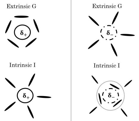
Figure 1: Galaxy shapes (ellipses) patterns for intrinsic (I) alignments and extrinsic gravitational (G) lensing. On the left column, we show the case of a massive structure at the center of the image: an overdensity $\delta_{+}$. On the right column, we show the case of a cosmic void: an underdensity $\delta_{-}$. The bottom panels assume a positive void bias.

In this work, we take the first steps towards the modelling and measurement of the alignments of the shapes of galaxies around voids using a sample of 3192 voids with redshifts $0.4<z<0.8$, and effective radii between 20 and 50 $h^{-1}$ Mpc. The study of alignments around cosmic voids is driven by two motivations. First, we expect that the assumption that galaxy shapes respond linearly to the tidal field should be very accurate. In other words, voids would offer an excellent environment where to test the linear model of galaxy alignments. This is motivated by the findings of Pollina et al. (2017), who demonstrated that the clustering of tracers around voids is very accurately described by a linear model, in contrast to the auto-correlation of the positions of those tracers. Second, we envisage that alignments of galaxies around voids could help constrain void properties such as their density profile, or their bias, and help enable some of their cosmological applications. Reischke & Schäfer 2019 already investigate the environmental dependence of the intrinsic ellipticity of spiral and elliptical galaxies, respectively, with a Gaussian random density field. The dependence on environment is modelled by the number of positive eigenvalues of the tidal tensor, which allows a differentiation between voids, sheets, filaments and superclusters. They find that alignment around voids is weak - an order of magnitude lower than for other environments. In this work, we develop our own theoretical model for alignment around voids, and contrast this against observations.

This paper is organized as follows. In section 2, we describe the linear alignment model along with our void-matter power-spectrum model. Section 3 describes the galaxy and void catalogues, and the estimator we use to measure the two-point correlation function. We present our results in section 4, analyze them in section 5 and conclude in section 6. For all of the model predictions, we use the following cosmology: $h=0.7$, $\Omega_{\text{CDM}}=0.225$, $\Omega_{\text{b}}=0.045$, $\Omega_{\Lambda}=0.73$, $\sigma_{8}=0.8$, $n_{s}=1$. We measure distances in $h^{-1}$ Mpc. This work used version 2.1 of the CCL library (Chisari et al., 2019) to compute essential cosmological functions, including matter power spectra derived from the CAMB software (Blas et al., 2011).

2 Formalism

2.1 Weak gravitational lensing

Working under the flat-sky approximation, we introduce a Cartesian frame defined by unit vectors $\hat{\bf e}_{x}$ and $\hat{\bf e}_{y}$ in the projected plane and $\hat{\bf e}_{z}$ along the line-of-sight. To describe the shape of a galaxy, we introduce two quantities: $\gamma_{1}$ and $\gamma_{2}$. $\gamma_{2}$ represents the stretching along $\hat{\bf e}_{x}$ and $\gamma_{1}$ along the axis $\hat{\bf e}_{x}$ rotated by $-45$ degrees.

In order to describe the shape relative to the separation vector between two points, corresponding to the coordinates of a galaxy and a void, we introduce the angle $\phi$ between this line and the $\hat{\bf e}_{x}$ axis. The shape in this frame is described by the rotation of $\gamma=(\gamma_{1},\gamma_{2})$ by an angle $2\phi$, as

$$\begin{split}\gamma_{+}&=-\cos(2\phi)\gamma_{1}-\sin(2\phi)\gamma_{2},\\ \gamma_{\times}&=\sin(2\phi)\gamma_{1}-\cos(2\phi)\gamma_{2}.\end{split}$$ (1)

Thus, a positive $\gamma_{+}$ corresponds to a radial alignment.

In practice, the ellipticity of a galaxy is measured as

$$(\epsilon_{+},\epsilon_{\times})=\frac{1-(b/a)^{2}}{1+(b/a)^{2}}(\cos(2\phi),\sin(2\phi)).$$ (2)

where $b$ is the length of the minor axis and $a$, the length of the major axis. For a given galaxy $i$, the observed shape can be decomposed in the initial ellipticity $\epsilon_{\text{source}}^{i}$, assumed to be random, an intrinsic ellipticity, $\gamma^{I}_{i}$, distorted by the large-scale structure, and the distortion due to weak lensing, $\gamma^{G}_{i}$ (see Hirata & Seljak 2004):

$$\epsilon_{\text{obs}}^{i}=\epsilon_{\text{source}}^{i}+\gamma^{I}_{i}+\gamma^{G}_{i}.$$ (3)

$\gamma^{I}_{i}$ and $\gamma^{G}_{i}$ are correlated with the overdensity of the matter field, $\delta$. Thus, taking the average over all observed galaxies,

$$\langle\delta\epsilon^{j}_{\text{obs}}\rangle=\langle\delta~{}\gamma^{I}_{j}\rangle+\langle\delta~{}\gamma^{G}_{j}\rangle.$$ (4)

Eq. (4) illustrates how intrinsic alignments act as a weak lensing contaminant.

2.2 Voids

The void density profile is well-described by the function (Hamaus et al., 2014b)

$$\Delta_{\mathrm{v}}(r)\equiv\frac{\rho_{\mathrm{v}}(r)}{\bar{\rho}_{\text{m}}}-1=\delta_{c}\frac{1-\left(r/r_{s}\right)^{\alpha}}{1+\left(r/r_{\mathrm{v}}\right)^{\beta}},$$ (5)

with 4 free parameters $\delta_{c}$, $r_{s}$, $\alpha$, $\beta$, and the measured void radius $r_{\mathrm{v}}$. $\delta_{c}<0$ is the central density contrast of the void, $\rho_{\mathrm{v}}$ and $\bar{\rho}_{\text{m}}$ are the matter density field around the void centre and its average background value, respectively. Spherical symmetry is warranted when one averages over a sufficiently large number of arbitrarily shaped voids with random orientations. For $r>2r_{\mathrm{v}}$, $\rho_{\mathrm{v}}(r)\approx\bar{\rho}_{\mathrm{m}}$, and the average void density profile quickly converges to the average density of the Universe. At the void centre, $\rho_{\mathrm{v}}(0)=\bar{\rho}_{\mathrm{m}}(1+\delta_{c})$, which represents a drop in density with respect to the average. $\Delta_{\mathrm{v}}$ is negative at the centre of the void but can change sign near $r\sim r_{\mathrm{v}}$ (Hamaus et al., 2014b). Far from the centre of the void, $\Delta_{\mathrm{v}}(r)\sim 0$ due to the convergence to the mean density of the Universe. Typical values of the free parameters in Eq. (5), derived from simulated mock catalogues, are: $(r_{s}/r_{\mathrm{v}},\alpha,\beta,\delta_{c})=(0.82,1.6,9.1,-0.36)$ (Hamaus et al., 2020). These parameters correspond to a population of mock galaxies with bias of $b_{\mathrm{g}}\approx 2.2$. For our sample (Table 1), we expect a slightly lower bias, about 1.85, and thus the value of $\delta_{c}$ could be slightly different than the one we assume.

2.3 Linear alignment model

Catelan et al. (2001) proposed a linear relation between the shape of a galaxy and the tidal field of the Universe, expressed as

$$\gamma_{+,\times}({\bf x})=-\frac{A_{I}C_{1}}{4\pi G}\left(\nabla_{x}^{2}-\nabla_{y}^{2}~{},~{}2\nabla_{x}\nabla_{y}\right)S\left[\Psi\right],$$ (6)

where $A_{I}C_{1}$ is a constant representing the response of a galaxy shape to a tidal deformation, and $S$ is a filter which cuts off fluctuations of the gravitational potential $\Psi$ at small scales. $C_{1}$ is retained for historical reasons: it is the value of the first intrinsic alignment measurement by Brown et al. (2002). Equivalently, in Fourier space,

$$\begin{split}\gamma_{+,\times}({\bf k})&=\frac{A_{I}C_{1}}{4\pi G}(k_{x}^{2}-k_{y}^{2},2k_{x}k_{y})\Psi\\ \end{split}$$ (7)

where $\Psi$ is the Fourier transform of the gravitational potential,

$$\begin{split}\Psi({\bf k})&=-4\pi G\frac{\bar{\rho}^{0}_{\text{m}}}{D(z)}\frac{\delta_{\text{m}}({\bf k})}{k^{2}}\end{split}$$ (8)

with $\bar{\rho}^{0}_{\text{m}}$, the mean density of the Universe at redshift $z=0$, and $D(z)$, the growth function (normalized to unity at $z=0$). The alignment bias can depend on many parameters such as the dynamical properties of a galaxy, its merger history, its redshift or its environment. Because this model is linear, it is only valid for large scales where the density fluctuations are small. We will neglect the filter $S$ in the rest of this work, because we will mainly focus on modelling linear scales where it does not have a significant impact.

2.4 Correlation functions

We introduce $\delta_{\text{m}}$, the matter overdensity, and $\delta_{\mathrm{v}}$, the void distribution,

$$\delta_{\text{m}}({\bf x}) =\left(\rho_{\text{m}}({\bf x})-\bar{\rho}_{\text{m}}\right)/\bar{\rho}_{\text{m}}$$ (9)

$$\delta_{\mathrm{v}}({\bf x}) =\frac{1}{N_{\mathrm{v}}^{\mathrm{tot}}}\sum_{i\in V}\delta^{(3)}(\bf x-\bf x_{i})$$ (10)

where $V$ is the void sample, $\delta^{(3)}$ is the Dirac function, $N_{\mathrm{v}}^{\mathrm{tot}}$ the number of voids and $\{\bf x_{i}\}$ are the void centres. The void-matter power spectrum is defined as the correlation of $\delta_{\text{m}}$ and $\delta_{\mathrm{v}}$ (Hamaus et al., 2014a),

$$\langle\delta_{\mathrm{v}}({\bf k})\delta_{\text{m}}({\bf k^{\prime}})\rangle=\delta^{(3)}({\bf k}-{\bf k^{\prime}})P_{\mathrm{vm}}({\bf k})(2\pi)^{3}.$$ (11)

The correlation functions between galaxy shapes and the void distribution are

$$\xi_{\mathrm{v}+}({\bf r}) =\langle\delta_{\mathrm{v}}({\bf x})\gamma_{+}({\bf x}+{\bf r})\rangle$$ (12)

$$\xi_{\mathrm{v}\times}({\bf r}) =\langle\delta_{\mathrm{v}}({\bf x})\gamma_{\times}({\bf x}+{\bf r})\rangle,$$ (13)

where $\langle\ldots\rangle$ represents an average over many realizations of the Universe. The void-intrinsic galaxy shape correlation is given by

$$\begin{split}\xi_{\mathrm{v}+}({\bf r})&=-\frac{A_{I}C_{1}\rho_{c}\Omega_{\text{m}}}{D(z)}\\ &\times\iint\frac{d^{3}kd^{3}k^{\prime}}{(2\pi)^{6}}\langle\delta_{\mathrm{v}}({\bf k})\delta_{\text{m}}({\bf k}^{\prime})\rangle\frac{k_{x}^{2}-k_{y}^{2}}{k^{2}}e^{i(k_{x}r_{p}+k_{z}\Pi)}.\end{split}$$ (14)

with $\Omega_{\text{m}}=\bar{\rho}^{0}_{\text{m}}/\rho_{c}$, $\rho_{c}$ being the critical density and ${\bf r}=r_{p}\hat{\bf e}_{x}+\Pi\hat{\bf e}_{z}$, with $r_{p}$ the component perpendicular to the line-of-sight, and $\Pi$ the component along the line-of-sight. The x-axis has been defined as the separation axis on the sky.

We can simplify Eq. (14) by integrating over the angle in $\vec{k}_{\perp}$ space, with $k_{\perp}=\sqrt{k_{x}^{2}+k_{y}^{2}}$. Using $k_{x}=k_{\perp}\cos(\theta)$ and $k_{x}^{2}-k_{y}^{2}=k_{\perp}^{2}\cos{(2\theta)}$, we recognize the second Bessel function $J_{2}$, and obtain the expression

$$\begin{split}\xi_{\mathrm{v}+}({\bf r})&=\frac{A_{I}C_{1}\rho_{c}\Omega_{\text{m}}}{\pi^{2}D(z)}\\ &\times\int_{0}^{\infty}\int_{0}^{\infty}dk_{\perp}dk_{z}P_{\mathrm{vm}}(k)\frac{k_{\perp}^{3}}{k^{2}}\cos(k_{z}\Pi)J_{2}(k_{\perp}r_{p}).\end{split}$$ (15)

Similarly, one can show that $\xi_{\mathrm{v}\times}=0$. Observational studies most often measure the projected correlation function, obtained by integrating Eq. (15) over the line-of-sight,

$$\omega_{X}(r_{p})=\int_{-\Pi_{\text{max}}}^{+\Pi_{\text{max}}}\xi_{X}(r_{p},\Pi)d\Pi,$$ (16)

with $X\in\{\mathrm{v}+,~{}\mathrm{v}\times\}$. We chose $\Pi_{\text{max}}$=150 $h^{-1}$ Mpc to ensure that we capture the alignments in the environments of voids. Obviously, $\omega_{\mathrm{v}\times}=0$, and

$$\begin{split}\omega_{\mathrm{v}+}(r_{p})=&\frac{A_{I}}{\pi^{2}}\frac{C_{1}\rho_{c}\Omega_{\text{m}}}{D(z)}\\ &\times\iint_{0}^{\infty}dk_{\perp}dk_{z}\frac{k_{\perp}^{3}}{k^{2}k_{z}}P_{\mathrm{vm}}(k)\sin(k_{z}\Pi_{\text{max}})J_{2}(k_{\perp}r_{p}).\end{split}$$ (17)

2.5 Window function and redshift-space distortions

Eq. (17) for $\omega_{\mathrm{v}+}$ was implicitly given at a specific redshift. We introduce $p_{\mathrm{v}}(z)\equiv 1/N_{\mathrm{v}}^{\text{tot}}dN_{\mathrm{v}}/dz$ and $p_{\mathrm{g}}(z)\equiv 1/N_{\mathrm{g}}^{\text{tot}}dN_{\mathrm{g}}/dz$, the redshift distributions of voids and galaxies, respectively, and the corresponding redshift window function (Mandelbaum et al., 2010):

$$W(z)=\frac{p_{\mathrm{v}}(z)p_{\mathrm{g}}(z)}{\chi^{2}d\chi/dz}\left(\int\frac{p_{\mathrm{v}}(z)p_{\mathrm{g}}(z)}{\chi^{2}d\chi/dz}dz\right)^{-1}.$$ (18)

We integrate Eq. (17) to yield the final prediction for the observable,

$$\begin{split}\omega_{\mathrm{v}+}(r_{p})=&\frac{A_{I}C_{1}\rho_{c}\Omega_{\text{m}}}{\pi^{2}}\int dz\frac{W(z)}{D(z)}\int_{0}^{+\infty}dk_{\perp}\int_{0}^{+\infty}dk_{z}\\ &\left\{\frac{k_{\perp}^{3}}{k^{2}k_{z}}P_{\mathrm{vm}}(k,z)\sin(k_{z}\Pi_{\text{max}})J_{2}(k_{\perp}r_{p})\right\}.\end{split}$$ (19)

One might consider a correction to Eq. (19) due to the presence of redshift-space distortions, first derived by Kaiser (1987) and consisting of a Doppler shift due to peculiar velocities. Including redshift-space distortions in our analysis would yield a correction smaller than 10 $\%$ at very large scales ($r_{p}\sim 100$ $h^{-1}$ Mpc). Since this correction is significantly smaller than the size of our error bars, we neglect it. Finally, as we restrict this study to galaxies in the immediate vicinity of voids ($<\,150\,h^{-1}$ Mpc), the lensing contribution is expected to be small.

2.6 Void-matter power spectrum

To determine the void-matter power spectrum, we will consider two regimes. The intermediate-scale regime will be used for scales $r_{p}\sim r_{\mathrm{v}}$, i.e. near the void boundary. A second regime will describe large scales, i.e. $r_{p}$ far enough from the void (typically $r_{p}>2r_{\mathrm{v}}$). We do not consider a small-scale regime $r_{p}\ll r_{\mathrm{v}}$, since by definition this region contains very few galaxies resulting in a large statistical uncertainty of our measurement. The combination of both models gives the alignment pattern of bottom-right panel of Figure 1 (for a positive void bias).

2.6.1 Intermediate-scale regime

For a single void of radius $r_{\mathrm{v}}$ centred at the origin, if $r\sim r_{\mathrm{v}}$, we can consider that the matter distribution is well-described by the void density profile, $\rho_{\mathrm{v}}(r)$. In this case, the void-matter two-point correlation is given by (Hamaus et al., 2015; Pollina et al., 2017)

$$\langle\delta_{\mathrm{v}}({\bf x}-{\bf 0})\delta_{\mathrm{m}}({\bf x}+{\bf r})\rangle=\frac{\rho_{\mathrm{v}}(r)}{\bar{\rho}_{\text{m}}}-1=\Delta_{\mathrm{v}}(r).$$ (20)

Thus, the power spectrum between void centres and the matter distribution at intermediate scales is (Chan et al., 2014)

$$\Delta_{\mathrm{v}}(k)\equiv P^{\mathrm{is}}_{\mathrm{vm}}(k)=\int_{0}^{+\infty}4\pi r^{2}dr\frac{\sin(kr)}{kr}\Delta_{\mathrm{v}}(r)$$ (21)

An empirical expression of $\Delta_{\mathrm{v}}$ in real space is obtained from simulations and only describes scales smaller and equivalent to the size of the void. To ensure the consistency of our separation of scales, we checked numerically that the contribution of the usual power spectrum with a cutoff at $k>\pi/2r_{v}$ (a basic model for large scale contamination) is negligible. Thus there is no large-scale contribution to Eq. (19) at $r_{p}\sim r_{\mathrm{v}}$. The mathematical reason for the large-scale contribution to be suppressed is that $J_{2}(k_{\perp}r_{p})$ kernel peaks near $k_{\perp}r_{p}\sim\pi$. This case is similar to the usual Limber approximation.

The power spectrum depends on the void radius, which motivates us to split our data into narrow radius intervals of 10 $h^{-1}$ Mpc. To account for potential mismatches between $\Delta_{\mathrm{v}}$ as predicted by simulations, and our observations, e.g. coming from different values of the density contrast of the voids, as detailed in Section 2.2, we introduce a free parameter $a_{\mathrm{v}}$ by assuming $\Delta_{\mathrm{v}}^{\text{data}}(k)=a_{\mathrm{v}}\Delta_{\mathrm{v}}^{\text{sim}}(k)$. For intermediate scales, we obtain the following model for the void-intrinsic shape correlation,

$$\begin{split}\omega_{\mathrm{v}+}(r_{p})=&A_{I}^{V}a_{\mathrm{v}}\frac{C_{1}\rho_{c}\Omega_{\text{m}}}{\pi^{2}}\int dz\frac{W(z)}{D(z)}\int_{0}^{+\infty}dk_{\perp}\int_{0}^{+\infty}dk_{z}\\ &\left\{\frac{k_{\perp}^{3}}{k^{2}k_{z}}\Delta_{\mathrm{v}}^{\text{sim}}(k)\sin(k_{z}\Pi_{\text{max}})J_{2}(k_{\perp}r_{p})\right\},\end{split}$$ (22)

with $A_{I}^{V}$ the alignment coefficient corresponding to void neighbourhood. Notice we have not considered any explicit redshift dependence in the parameters that characterize the voids, and we instead hold them constant over our redshift range of interest, $0.4<z<0.8$.

2.6.2 Large-scale regime

The void-matter power spectrum can be split into two terms (Chan et al., 2014),

$$\begin{split}P_{\mathrm{vm}}(k)=&\int_{0}^{+\infty}dr\,4\pi r^{2}\frac{\sin(kr)}{kr}\left[\Delta_{\mathrm{v}}(r)-b_{\mathrm{v}}(r_{\mathrm{v}})\xi_{\mathrm{mm}}^{\text{lin}}(r)\right]\\ &+b_{\mathrm{v}}(r_{\mathrm{v}})\int_{0}^{+\infty}dr\,4\pi r^{2}\frac{\sin(kr)}{kr}\xi_{\mathrm{mm}}^{\text{lin}}(r),\end{split}$$ (23)

where $b_{\mathrm{v}}$ is the void bias (Hamaus et al., 2014a), and $\xi^{\text{lin}}_{\mathrm{mm}}$ is the matter correlation function predicted from linear theory.

In the large-scale limit, the void-matter power spectrum should approach the shape of the matter-matter power spectrum. This implies there exists a radius $r_{\star}$ such that $\Delta_{\mathrm{v}}(r>r_{\star})=b_{\mathrm{v}}(r_{\mathrm{v}})\xi_{\mathrm{mm}}^{\text{lin}}(r)$. Therefore, Eq. (23) can be simplified to

$$\begin{split}P^{\mathrm{ls}}_{\mathrm{vm}}(k)=&\int_{0}^{r_{\star}}dr\,4\pi r^{2}\frac{\sin(kr)}{kr}\left[\Delta_{\mathrm{v}}(r)-b_{\mathrm{v}}(r_{\mathrm{v}})\xi_{\mathrm{mm}}^{\text{lin}}(r)\right]\\ &+b_{\mathrm{v}}(r_{\mathrm{v}})P_{\mathrm{mm}}^{\text{lin}}(k).\end{split}$$ (24)

For small wave vectors (large scales), the first term can be neglected, and we recover the familiar linear bias result,

$$P^{\mathrm{ls}}_{\mathrm{vm}}\left(k<\frac{2\pi}{r_{\mathrm{v}}}~{}~{}|r_{\mathrm{v}},~{}z\right)=b_{\mathrm{v}}(r_{\mathrm{v}})P_{\mathrm{mm}}^{\text{lin}}(k,z).$$ (25)

Here again, the power spectrum depends on void radius (as $b_{\mathrm{v}}$ does), which justifies our selection of void radius intervals of 10 $h^{-1}$ Mpc for the large-scale measurements. The resulting projected correlation function in the large-scale regime is given by

$$\begin{split}\omega_{\mathrm{v}+}(r_{p})=&A_{I}^{V}b_{\mathrm{v}}(r_{\mathrm{v}})\frac{C_{1}\rho_{c}\Omega_{\text{m}}}{\pi^{2}}\int dz\frac{W(z)}{D(z)}\int_{0}^{+\infty}dk_{\perp}\int_{0}^{+\infty}dk_{z}\\ &\left[\frac{k_{\perp}^{3}}{k^{2}k_{z}}P_{\mathrm{mm}}^{\text{lin}}(k,z)\sin(k_{z}\Pi_{\text{max}})J_{2}(k_{\perp}r_{p})\right].\end{split}$$ (26)

3 Methodology

3.1 Data sets

We introduce the following notations for samples used in this work. $V$ represents the void sample positions and $R_{V}$, the corresponding randoms. $S_{+}$ represents the shapes and positions of the sample of galaxies, and $R_{S}$, the corresponding randoms.

3.1.1 Galaxy positions and shapes

We use a sample of galaxies from data release 12 (DR12) of the SDSS-III Baryon Oscillation Spectroscopic Survey (BOSS, Eisenstein et al. 2011). We consider the CMASS sample: massive galaxies at redshift $0.4<z<0.8$. We use the catalogue of galaxy shapes complied by Singh et al. (2021) by matching the CMASS sample with the galaxy shape measurements from Reyes et al. (2012). We also make use of the random catalogue provided by the BOSS collaboration, which is a realization of an unclustered galaxy distribution with the same survey geometry (mask). We use 13 times more random points than galaxies at any given redshift to avoid the size of the random catalogue having an impact on the observables.

3.1.2 Void positions

The void catalogue is obtained using the vide software (Sutter et al., 2015) applied to the combined sample of DR12 BOSS galaxies previously used in Hamaus et al. (2020). vide is based on zobov (Neyrinck, 2008), an algorithm that identifies voids by searching for “basins” in the density field of the observed tracers. Each location within the survey volume is attributed to its closest tracer (i.e., a galaxy). This operation defines a Voronoi tessellation with cells of volume $\mathcal{V}_{i}$ for each tracer $i$. The density field of tracers $\rho({\bf x})$ at any given location ${\bf x}$ inside the survey volume is then estimated by evaluating $1/\mathcal{V}_{i}$. vide identifies voids as watershed basins of arbitrary shape, uncovering extended underdense regions that are surrounded by overdense boundaries. Every Voronoi cell contained in such a basin is then considered as part of a void.

The location of the void centre ${\bf X}$ is defined as the volume-weighted barycentre among all of its constituent Voronoi cells: ${\bf X}=\sum_{i}{\bf x}_{i}\mathcal{V}_{i}/\sum_{i}\mathcal{V}_{i}$, where ${\bf x}_{i}$ is the location of each tracer that defines the void. The effective void radius is defined as $r_{\mathrm{v}}=(3/4\pi\sum_{i}\mathcal{V}_{i})^{1/3}$. The galaxy and void catalogues cover the same region of the sky and redshift range. In Figure 2, we present their redshift distributions, which are very similar over the CMASS redshift range. Voids appear equally distributed within that galaxy sample.

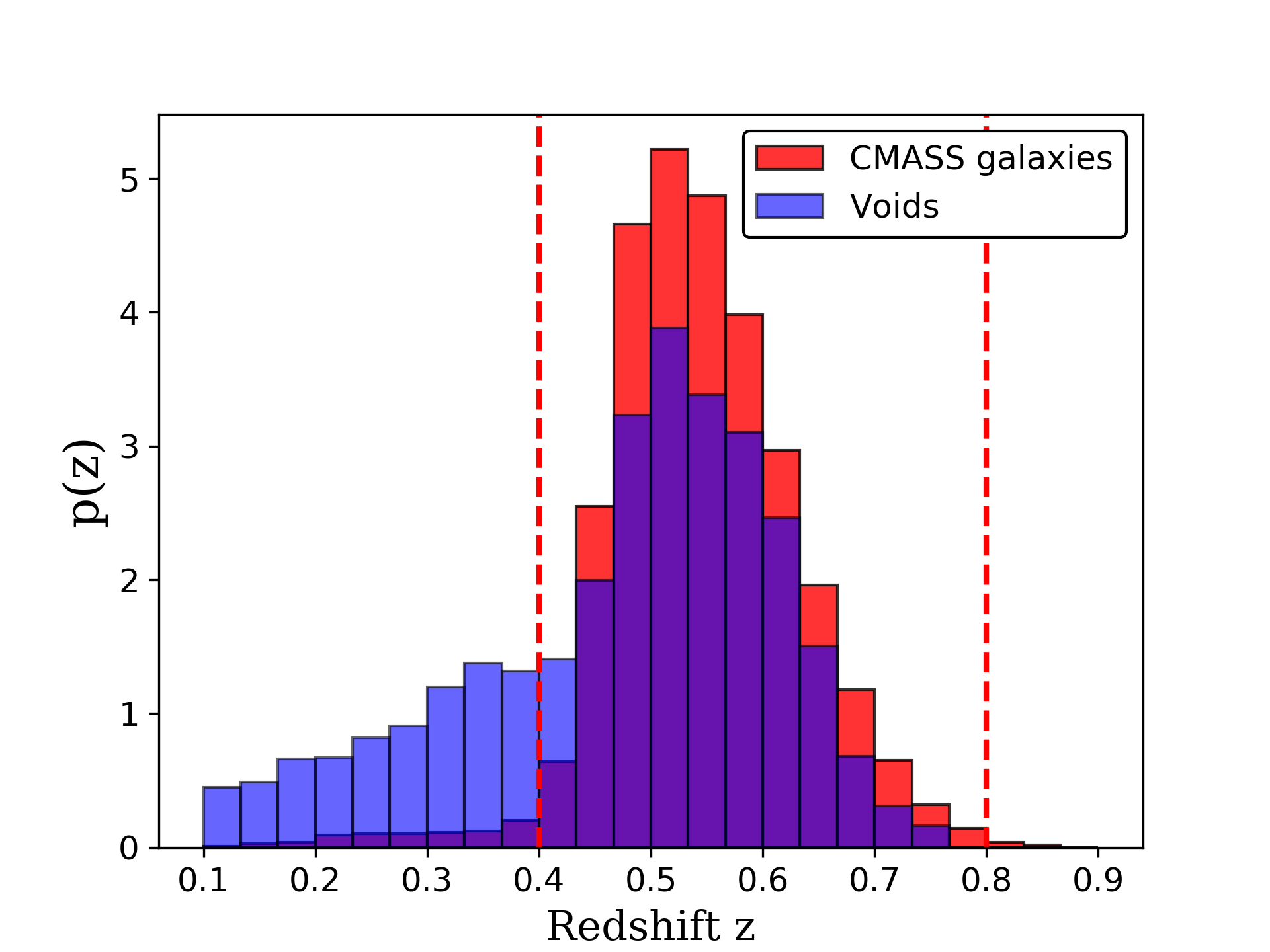
Figure 2: Redshift distribution of CMASS galaxies (red) and voids (blue). Red dashed lines represent the redshift range used in our study. The distribution is normalized such that $\int_{z}p(z)dz=1$. The presence of voids at $z<0.4$ is due to the catalogue being constructed from the full DR12 BOSS data. In practice, we are only interested in cross-correlations between physically close pairs of galaxies and voids.

Finally, we use a random catalogue for void positions, $R_{V}$, which has been generated with same redshift and void radii distributions, and takes into account the survey mask. This random catalogue is 10 times larger than the void one.

3.2 Estimators

We measure the correlation function of void positions and galaxy shapes using a Landy-Szalay estimator (Landy & Szalay, 1993),

$$\xi_{\mathrm{v}+}(r)=\frac{VS_{+}-R_{V}S_{+}}{R_{V}R_{S}}$$ (27)

where the terms $VS_{+}$, $R_{V}S_{+}$ and $R_{V}R_{S}$ stand for the sums

$$\begin{split}VS_{+}(r_{p},\Pi)&=\sum_{\begin{subarray}{c}i\in S,j\in V\\ |i-j|=r_{p},\Pi\end{subarray}}\gamma_{+}^{(i)}\langle i|j\rangle\\ R_{V}S_{+}(r_{p},\Pi)&=\sum_{\begin{subarray}{c}i\in S,j\in R_{V}\\ |i-j|=r_{p},\Pi\end{subarray}}\gamma_{+}^{(i)}\langle i|j\rangle\end{split}$$ (28)

where $\gamma_{+}^{(i)}\langle i|j\rangle$ denotes the $+$ shape of a galaxy $i$ relative to void $j$. $R_{V}R_{S}(r_{p},\Pi)$ is the number of pairs of random voids and random galaxies that are separated by $r_{p}$ and $\Pi$. We numerically normalize the terms $R_{V}S_{+}$ and $R_{V}R_{S}$ to account for the relative size of random and galaxy catalogues.

To obtain the projected correlation function, we divide the line-of-sight interval into $n$ bins of length $2\Delta\Pi^{(m)}$ and centred at $\Pi^{(m)}$,

$$\omega_{\mathrm{v}+}(r_{p})\approx\sum_{m=1}^{n}\xi_{\mathrm{v}+}(r_{p},\Pi^{(m)})2\Delta\Pi^{(m)}.$$ (29)

The different samples used in the estimation of the correlation functions are described in Table 1. We divide the void sample according to their sizes in intervals of small voids: $[20,30]\,h^{-1}$ Mpc, intermediate voids: $[30,40]\,h^{-1}$ Mpc and large voids: $[40,50]\,h^{-1}$ Mpc. The choice of minimum radius is driven by the fact that smaller voids are surrounded by overdensities (e.g. clusters) which can induce a very strong correlation and wash out the void signal. We also had at our disposal voids with a radius larger than 50 $h^{-1}$ Mpc, but the number of these voids per interval of 10$h^{-1}$ Mpc is significantly smaller. Since our measurements are already not significant for the voids with radii in 40-50 $h^{-1}$Mpc range, we did not extend this study to these larger voids.

Sample	Small voids	Intermediate voids	Large voids	Galaxies
	$r_{\mathrm{v}}=[20,30]\,h^{-1}$ Mpc	$r_{\mathrm{v}}=[30,40]\,h^{-1}$ Mpc	$r_{\mathrm{v}}=[40,50]\,h^{-1}$ Mpc
Data	1089	1220	883	560011
Random	11777	12021	8485	7828387

Table 1: Characteristics of the various samples used in estimating the correlation function of galaxies around voids (Eq. 29). All samples span the redshift range $0.4<z<0.8$.

3.3 Covariance matrix

We use the jackknife method to obtain estimates of the covariance matrix and error bars for the projected correlation function of void positions and galaxy shapes. We split the observed area of the sky into $N_{\text{reg}}$ sub-regions taking the survey mask into account. We measure a set of projected correlation functions, $\tilde{\omega}_{\mathrm{v}+}^{i}(r_{p})$, by removing one sub-region $i$ at a time. We define $\bar{\omega}_{\mathrm{v}+}(r_{p})$ as the mean of $\tilde{\omega}_{\mathrm{v}+}^{i}(r_{p})$. The covariance matrix $\mathcal{C}[r_{p}^{i},r_{p}^{j}]$ is estimated via

$$\mathcal{C}[r_{p}^{i},r_{p}^{j}]=\frac{N_{\text{reg}}-1}{N_{\text{reg}}}\sum_{k=1}^{N_{\text{reg}}}\left[\tilde{\omega}^{k}(r_{p}^{i})-\bar{\omega}_{\mathrm{v}+}(r_{p}^{i})\right]\left[\tilde{\omega}^{k}(r_{p}^{j})-\bar{\omega}_{\mathrm{v}+}(r_{p}^{j})\right].$$ (30)

The diagonals represent the error bars shown in the figures, $\sigma(r_{p}^{i})=\sqrt{\mathcal{C}[r_{p}^{i},r_{p}^{i}]}$. These expressions provide accurate estimates of the uncertainty in the estimated projected correlation function, if sub-regions satisfy the following properties:

1. the sub-volume sizes are larger than the biggest scale probed in the observable,

2. $N_{\text{reg}}$ is larger than the number of bins where the projected correlation function is estimated, and

3. the number of data points (e.g. voids and galaxies) in each sub-volume is approximately the same.

As the number of voids is limited (a few thousand), in order for them to be distributed equally among the sub-regions, the number of sub-regions must be kept small. We use 64 sub-regions as a compromise to meet the above conditions. To determine the actual sub-regions, we use a $K$-means algorithm on the sphere to find maximally separated centres in a RA and DEC distribution of randoms $R_{S}$. The choice of $R_{S}$ (vs. $R_{V}$) for determining the jackknife sub-regions is due to higher sampling and justified by the fact that the voids are selected from the same galaxy sample.

3.4 Model fits

We perform a $\chi^{2}$ minimization in order to obtain constraints for the free parameters of the models. For a given free parameter $a$, we minimize the function

$$\chi^{2}(a)=\left[\bar{\omega}_{\mathrm{v}+}-\omega_{\mathrm{v}+}^{\text{model}}(a)\right]\mathcal{C}^{-1}\left[\bar{\omega}_{\mathrm{v}+}-\omega_{\mathrm{v}+}^{\text{model}}(a)\right]^{\top}.$$ (31)

The best fit corresponds to the minimal value of $\chi^{2}$: $\chi^{2}_{\text{model}}$. The confidence interval is determined by the requirement that

$$\chi^{2}(x)<\chi^{2}_{\text{model}}+\delta\chi^{2},$$ (32)

with $\delta\chi^{2}$ depending on the number of free parameters and the confidence level. We report $68\%$ confidence levels as default, which sets $\delta\chi^{2}=1$ for 1 free parameter. We also calculate the $\chi^{2}$ value for the null model: $\chi^{2}_{0}$, and the difference between both

$$\Delta\chi^{2}=\chi^{2}_{0}-\chi^{2}_{\text{model}}\geq 0.$$ (33)

From $\chi^{2}_{\text{model}}$, $\chi^{2}_{0}$ and $\Delta\chi^{2}$, we calculate three p-values $p_{\text{model}}$, $p_{0}$ and $p_{\Delta}$. $p_{\text{model }}$ and $p_{0}$ evaluate the rejection or not of the model, and the null hypothesis, by the data. $p_{\Delta}$ gives an assessment on the significance of goodness of the best fit in comparison to the null hypothesis.

4 Results

We restrict our measurements of the projected correlation (Eq. 29) to scales $r_{p}>10\,h^{-1}$ Mpc. Smaller scales are affected by large error bars due to a paucity of galaxy-void pairs given the intrinsic low density of these environments (Sutter et al., 2014). The intermediate-scale model (Eq. 22) is fit at $r_{p}<1.5r_{\mathrm{v}}$, and the large-scale model (Eq. 26) is adopted when $r_{p}>2r_{\mathrm{v}}$. We thus obtain a constraint for the free coefficients of each model: $A_{I}^{V}a_{\mathrm{v}}$ at intermediate scales (introduced in section 2.6.1) and $A_{I}b_{\mathrm{v}}(r_{\mathrm{v}})$ at large scales (introduced in section 2.6.2). The bias of the voids depends on their radius (Hamaus et al., 2014a), so we expect different values for each measurement.

A summary of our results is presented in Table 2 and discussed in the following subsections. In Appendix B we show results for $\omega_{\mathrm{v}\times}$ to check its consistency with a null signal, which corresponds to a non-zero $p$-value. These measurements confirm that for $r_{\mathrm{v}}\in\,20-30$ and $30-40\,h^{-1}$ Mpc, there is no ${\times}$ correlation. For larger voids, we find a small $p$-value ($p_{0}<0.01$), which means that $\omega_{\mathrm{v}\times}$ is not consistent with the null hypothesis. We give some possible explanation of this measure in B.3, and will not exploit in detail the $+$ correlation for large voids since it might be affected by systematics.

Combining the three void sample measurements, we find no significant deviation from the null hypothesis for either intermediate- and large-scale regimes ($p_{0}=0.41$), the large-scale regime ($p_{0}=0.25$), or the intermediate-scale regime ($p_{0}=0.60$).

$r_{\mathrm{v}}$ [$h^{-1}$ Mpc]	Regime	$\#$points	Scales fit [$h^{-1}$ Mpc]	$\chi_{\text{model}}^{2}$	$p_{\text{model}}$	$\chi_{0}^{2}$	$p_{0}$	$\Delta\chi^{2}$	$p_{\Delta}$	Bias factors
$[20,30]$	Intermediate scales	6	10-36	10.0	0.075	11.3	0.046	1.3	0.93	$A_{I}^{V}a_{\mathrm{v}}=-123\pm 105$
$[20,30]$	Large scales	5	46-127	2.0	0.74	9.3	0.054	7.3	0.12	$A_{I}b_{\mathrm{v}}=27.0\pm 11.1$
$[30,40]$	Intermediate scales	7	10-46	1.7	0.94	4.1	0.63	2.4	0.88	$A_{I}^{V}a_{\mathrm{v}}=75\pm 45$
$[30,40]$	Large scales	4	60-127	0.88	0.83	5.8	0.11	4.9	0.18	$A_{I}b_{\mathrm{v}}=18.4\pm 8.2$
$[40,50]$	Intermediate scales	8	10-60	2.2	0.99	2.4	0.94	0.2	1	$A_{I}^{V}a_{\mathrm{v}}=-13\pm 31$
$[40,50]$	Large scales	3	77-127	0.76	0.68	0.82	0.66	0.06	0.97	$A_{I}b_{\mathrm{v}}=-3.9\pm 16.1$

Table 2: Results of intrinsic alignment amplitude fits from $\omega_{\mathrm{v}+}$ measurements in both regimes and for the different void radius ranges. Columns 5 and 6 indicate the quality of the best fit via the chi-squares and p-values. Columns 7 and 8 show the corresponding values for the null hypothesis (no signal). Column 9 provides $p_{\Delta}$, the probability for rejection of the null hypothesis, assuming the model is valid.

4.1 Small voids

The measurement of $\omega_{\mathrm{v}+}$ for this sample of voids is shown in Fig. 3, along with the resulting large-scale model fit, applied to scales $r_{p}>46\,h^{-1}$ Mpc (5 points). We do not show the best fit with the intermediate-scale model, because it has been rejected by the data at $1.8\sigma$ : $p_{\text{model}}=0.075$. The null hypothesis is rejected at 2$\sigma$ for both fit ranges ($p_{0}\sim$ 0.05 for both regimes).
For the large-scale model, we find $A_{I}b_{\mathrm{v}}(r_{\mathrm{v}})=27.0\pm 11.1$, with $p_{\text{model}}=0.74$. Here, the large-scale model describes the measurements well. Nonetheless, $p_{\Delta}=0.12$, which means that the significance for a detection of the alignment is lower than 1.5$\sigma$.

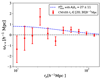
Figure 3: $\omega_{\mathrm{v}+}$ with $r_{\mathrm{v}}=[20,30]\,h^{-1}$ Mpc, and the large-scale prediction with $A_{I}b_{\mathrm{v}}=27.0\pm 11.1$. The intermediate-scale model is rejected, and we did not include it in the plot.

4.2 Intermediate voids

We use the intermediate-scale model for $10h^{-1}\mathrm{Mpc}<r_{p}<46h^{-1}\mathrm{Mpc}$ (7 points) and the large-scale one for $r_{p}>60h^{-1}\mathrm{Mpc}$ (4 points) for the intermediate-size voids. The measurements and both models are shown in Fig. 4. The null hypothesis is rejected at 1.5$\sigma$ on large scales ($p_{0}=0.11$), but it is not rejected at small scales ($p_{0}=0.63$).
In the intermediate-scale regime, we find $A_{I}^{V}a_{\mathrm{v}}=75\pm 45$, with $p_{\text{model}}=0.94$ confirming a good fit. Nonetheless, since $p_{\Delta}=0.88$, our model is not significantly better than the null one. In the large-scale regime, we find $A_{I}b_{\mathrm{v}}(r_{\mathrm{v}})=18.4\pm 8.2$, with $p_{\text{model}}=0.83$. The detection of the alignment is not statistically significant, since $p_{\Delta}=0.18$.

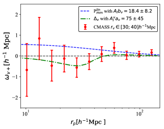
Figure 4: $\omega_{\mathrm{v}+}$ with $r_{\mathrm{v}}\in[30;40]\,h^{-1}$ Mpc, the intermediate-scale prediction with $A_{I}^{V}a_{\mathrm{v}}=75\pm 45$, and the large-scale one with $A_{I}b_{\mathrm{v}}=18.4\pm 8.2$.

4.3 Large voids

We use the intermediate-scale model for $r_{p}<60$ $h^{-1}$Mpc (8 points) and the large-scale one for $r_{p}>77$ $h^{-1}$Mpc (3 points). The measurement is shown in Figure 5, with the resulting large-scale model overlaid. Here again, we do not show the intermediate-scale one, because there is no distinction between the best fit, and the null one: $p_{\Delta}=1$. The null hypothesis is not excluded at both scales: $p_{0}=0.94$ for intermediate scales and $p_{0}=0.66$ for large scales.
On large scales, we find $A_{I}b_{\mathrm{v}}(r_{\mathrm{v}})=-3.9\pm 16.1$, with $p_{\text{model}}=0.68$. There is almost no distinction between the best fit and the null hypothesis, since $p_{\Delta}=0.97$.

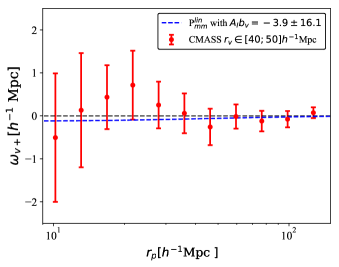
Figure 5: $\omega_{\mathrm{v}+}$ with $r_{\mathrm{v}}\in[40;50]h^{-1}\mathrm{Mpc}$, and the large-scale prediction with $A_{I}b_{\mathrm{v}}=-3.9\pm 16.1$. The signal at intermediate scales is too noisy to have a detection of alignments in the intermediate-scale regime.

5 Discussion

Following our modelling, we expect to detect two distinct regimes:

• at intermediate scales, due to the proximity of the void, the correlation should be negative, i.e. the galaxies align tangentially;

• at larger scales, the alignment depends on the value of the void bias; for positive bias, the galaxies align radially (pattern of figure 1); for negative bias, they align tangentially.

However, these effects, especially for the intermediate scales, are supposed to be weak and therefore difficult to detect; especially since we have a limited sample of only a few thousand voids.

For voids with radii between 20 and 30$h^{-1}\mathrm{Mpc}$, we measured alignments that were compatible with no signal at 2$\sigma$. For these voids we also do not measure any signature of the void contribution at intermediate scales. This may be due to the tendency of these voids to contain more tracers at their boundary. At large scales, we find an IA amplitude of $A_{I}b_{\mathrm{v}}(25\,h^{-1}\text{Mpc})\sim 27\pm 11.1$. This is an acceptable order of magnitude, since we expect $A_{I}\sim 5$ as for LOWZ and CMASS (Singh et al. 2015, 2021), which would mean that we have a void bias around 2-6, (in order of magnitude similar to Clampitt et al. 2016). The analysis of the $\times$ correlation between shapes and voids in appendix B.1 confirms that this is compatible with null ($p_{0}=0.96$), as expected.

For voids with intermediate sizes, the null hypothesis at large scales is almost excluded by the p-value test ($p_{0}=0.11$), but it is not excluded at intermediate scales ($p_{0}=0.63$). Given the noise, and the fact that even the model only deviates from 0 at a small interval at $r_{p}$ close to $r_{\mathrm{v}}$, it is not surprising to obtain a high $p$-value for the null hypothesis, and we were not able to distinguish statistically the null model from the best fit one: $p_{\Delta}=0.88$. At large scales, the model agrees relatively well with the measurement, with a measured IA coefficient $A_{I}b_{\mathrm{v}}(35\,h^{-1}\text{Mpc})\sim 18.4\pm 8.2$. We find here again a physically acceptable order of magnitude. Since $A_{I}$ is the same as in the first measurement (we are working with the same galaxy shape sample), the void bias for $r_{\mathrm{v}}\sim 35\,h^{-1}$ Mpc appears to be smaller than the one for $r_{\mathrm{v}}\sim 25\,h^{-1}$ Mpc. A trend of decreasing bias with increasing void radius has already been suggested by Hamaus et al. (2014a); Chan et al. (2014); Jamieson & Loverde (2019); Chan et al. (2020) from simulations. The analysis of the $\times$ correlation between shapes and voids in appendix B confirms again that this is compatible with null as expected, with $p_{0}=0.17$.

Finally, the intrinsic alignments of CMASS galaxies around large voids are compatible with null ($p_{0}=0.66$ for large scales and $p_{0}=0.94$ for intermediate scales). Moreover, the $\times$ correlation between shapes and voids, presented in appendix B.3, is not compatible with 0 ($p_{0}=9\times 10^{-4}$), which could indicate that the measurements are not reliable. This may be due to the smaller number of large voids, and their more complex sub-structure, which could break the assumption of spherical symmetry. It is also possible that at large scales the null measurement of the $+$ correlation is due to a void bias close to 0, which is typical for compensated voids (Hamaus et al., 2014a).

6 Conclusion and perspectives

We have studied intrinsic alignments of galaxies around cosmic voids, in SDSS-III BOSS CMASS galaxies. Using this sample, we have investigated the shape-position correlation from 10 to 140 $h^{-1}$ Mpc scales, binning voids by size.

Our model suggests the existence of two regimes: for scales equivalent to the void radius, the correlation should be negative, which means that galaxies align tangentially. At large scale, for positive void bias, the correlation should be positive, which implies a radial alignment for galaxies (negative bias implies a tangential alignment). The intermediate-scale regime with the negative correlation is more difficult to observe, because the available number of galaxies close to the void centre is small. However, it may be the most interesting one in order to extract physical information and constraints, since it directly depends on the mass distribution inside voids.

We find that the large-scale model fits well data for void radius ranges: 20-30 $h^{-1}$ Mpc and 30-40 $h^{-1}$ Mpc, giving constraints for the void bias. For the void radius range 40-50 $h^{-1}$ Mpc, the measurement is consistent with 0 at any scale. For the large-scale part, it may be the consequence of a vanishing void bias. Furthermore, we find a significant null model deviation for the $\times$ correlation, which implies to be careful with this last measurement.

For the intermediate-scale regime, as expected, the noise is the main limit for the detection of a correlation. Our intermediate-scale model seems ineffective to describe the measurement for 20-30 $h^{-1}$ Mpc and 40-50 $h^{-1}$ Mpc void radius ranges, because the model is rejected by data for smaller voids, and equivalent compatible with null for larger voids. Keeping only voids with radius between 30 and 40 $h^{-1}$ Mpc, we achieve a tentative detection of a negative correlation in agreement with the predictions of our intermediate-scale model. Smaller voids are more clustered than bigger ones, which may lead to a strong positive correlation coming from high-density environments. In such a case, the contribution from the voids would be hard to detect. Large voids are not very numerous, which combined with an important proportion of voids being elongated and featuring sub-structure, may contradict the spherical symmetry assumption of our model and may lead to biased measurements. Furthermore, voids with radius between 30-40 $h^{-1}$ Mpc are the most abundant, which helps to increase the signal-to-noise ratio and reduce potential systematics coming from small-number statistics.

The number of voids is supposed to drastically increase with future surveys by about two orders of magnitude (Pisani et al., 2019), which will necessarily lead to a substantial reduction of the noise due to the noise contribution to the covariance scaling directly with the inverse of the number density for both voids and galaxy shapes.

Thus, future surveys will allow us to confirm or rule out the tentative detection of a negative alignment correlation at intermediate scale for voids of all sizes. With a noise reduction, it would also be possible to make a joint analysis with other correlations to remove the degeneracies of the coefficients, and extract physical constraints.

In anticipation, we plan to investigate the validity of our model with numerical simulations. This could open the door for new applications of intrinsic alignments and for calculating their contamination to void lensing studies with photometric or spectroscopic galaxy samples (e.g., Clampitt & Jain, 2015; Sánchez et al., 2016; Fang et al., 2019).

Data availability

No new data were generated or analysed in support of this research. The shape catalogue was presented in Singh et al. (2021) and the void catalogue, in Hamaus et al. (2020).

Appendix A Impact of density-weighting of galaxy shapes

The ${\gamma}^{I}$ field is not uniformly sampled by observations. Rather, we sample it at the locations of galaxies. Thus in reality, we observe

$$\tilde{\gamma}^{I}=(1+b_{\mathrm{g}}\delta)\gamma^{I}.$$ (34)

Using Fourier transformation on $\tilde{\gamma}^{I}$, we obtain an integral expression,

$$\begin{split}&\tilde{\gamma}^{I}({\bf k}~{},~{}z)=-\frac{C_{1}\bar{\rho}_{\text{m}}}{D(z)}\iiint d^{3}k_{1}\\ &\left\{\left(k_{2x}^{2}-k_{2y}^{2}~{},~{}2k_{2x}k_{2y}\right)\delta({\bf k_{2}},z)\left(\delta^{(3)}({\bf k_{1}})+b_{\mathrm{g}}\delta({\bf k_{1}}~{},~{}z)\right)\right\},\end{split}$$ (35)

with $\bf k_{2}=k-k_{1}$. Here, we directly see that in the Fourier space,

$$\langle\delta_{\mathrm{v}}\tilde{\gamma_{I}}\rangle=\langle\delta_{\mathrm{v}}\gamma_{I}\rangle+\mathcal{O}(\delta_{\mathrm{v}}\delta_{\mathrm{m}}^{2})$$ (36)

Thus, if we restrict our study to linear order, we can omit the correction to $\gamma_{I}$.

Appendix B $\times$ correlation

We present here the measurements of the $\times$ correlation, which we expect to be consistent with a null signal. Otherwise, it could be a possible indication that systematics affect the measurement. We estimate the $\times$ correlation using Eq. (27), with $S_{\times}$ instead of $S_{+}$. We compute the $p$-value for each measurement (corresponding to different void radii), and summarize the results in Table 3.

$r_{\mathrm{v}}$ [$h^{-1}$ Mpc]	$p_{0}$
[20-30]	$0.96$
[30-40]	$0.17$
[40-50]	$0.0009$

Table 3: Table of the p-values of the null hypothesis for the $\times$ correlation.

B.1 Void radius in 20-30 $h^{-1}$ Mpc range

The measurement is presented in figure 6. For small voids, we find a $p$-value compatible with a null signal: $p_{0}=0.96$.

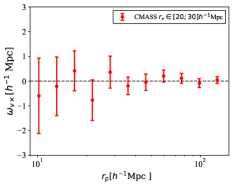
Figure 6: $\times$ correlation for voids with $r_{\mathrm{v}}\in$ 20-30 $h^{-1}$ Mpc.

B.2 Void radius in 30-40 $h^{-1}$ Mpc range

The measurement is presented in figure 7. We find a $p$-value quite compatible with a null signal: $p_{0}=0.16$, even if its value is lower than for smaller voids, mainly because of the positive trend at $r_{p}\sim 10h^{-1}\mathrm{Mpc}$.

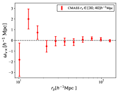
Figure 7: $\times$ correlation for voids with $r_{\mathrm{v}}\in$ 30-40 $h^{-1}$ Mpc.

B.3 Void radius in 40-50 $h^{-1}$ Mpc range

The measurement is presented in figure 8. For large voids, we find a $p$-value that suggests the rejection of the null hypothesis: $p_{0}=0.0009$. The measurements for these voids are not exploited in detail in the analysis presented in the main body of the manuscript, since they may be subject to systematics. It is also possible that we detect a non-vanishing signal due to important sub-structure inside voids, and the void sample could not be large enough to average out their contribution. Alternatively, the error bars could be underestimated.

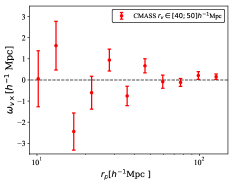
Figure 8: $\times$ correlation for voids with $r_{\mathrm{v}}\in$ 40-50 $h^{-1}$ Mpc.

References

- Achitouv (2019) Achitouv I., 2019, Phys. Rev. D, 100, 123513
- Aihara et al. (2017) Aihara H., et al., 2017, Publications of the Astronomical Society of Japan, 70
- Amendola et al. (2018) Amendola L., et al., 2018, Living Reviews in Relativity, 21
- Aubert et al. (2020) Aubert M., et al., 2020, The Completed SDSS-IV Extended Baryon Oscillation Spectroscopic Survey: Growth rate of structure measurement from cosmic voids (arXiv:2007.09013)
- Baker et al. (2018) Baker T., Clampitt J., Jain B., Trodden M., 2018, Physical Review D, 98
- Baldi & Villaescusa-Navarro (2017) Baldi M., Villaescusa-Navarro F., 2017, Monthly Notices of the Royal Astronomical Society, 473, 3226
- Banerjee & Dalal (2016) Banerjee A., Dalal N., 2016, Journal of Cosmology and Astroparticle Physics, 2016, 015
- Barreira et al. (2015) Barreira A., Cautun M., Li B., Baugh C. M., Pascoli S., 2015, Journal of Cosmology and Astroparticle Physics, 2015, 028–028
- Bernstein & Jarvis (2002) Bernstein G. M., Jarvis M., 2002, AJ, 123, 583
- Biagetti & Orlando (2020) Biagetti M., Orlando G., 2020, J. Cosmology Astropart. Phys., 2020, 005
- Blas et al. (2011) Blas D., Lesgourgues J., Tram T., 2011, JCAP, 7, 34
- Blazek et al. (2011) Blazek J., McQuinn M., Seljak U., 2011, Journal of Cosmology and Astroparticle Physics, 2011, 010–010
- Brown et al. (2002) Brown M. L., Taylor A. N., Hambly N. C., Dye S., 2002, Monthly Notices of the Royal Astronomical Society, 333, 501
- Cai et al. (2016) Cai Y.-C., Taylor A., Peacock J. A., Padilla N., 2016, Monthly Notices of the Royal Astronomical Society, 462, 2465
- Catelan et al. (2001) Catelan P., Kamionkowski M., Blandford R. D., 2001, Monthly Notices of the Royal Astronomical Society, 320, L7–L13
- Chan et al. (2014) Chan K. C., Hamaus N., Desjacques V., 2014, Physical Review D, 90
- Chan et al. (2019) Chan K. C., Hamaus N., Biagetti M., 2019, Phys. Rev. D, 99, 121304
- Chan et al. (2020) Chan K. C., Li Y., Biagetti M., Hamaus N., 2020, The Astrophysical Journal, 889, 89
- Chen et al. (2015) Chen Y.-C., Ho S., Freeman P. E., Genovese C. R., Wasserman L., 2015, Monthly Notices of the Royal Astronomical Society, 454, 1140–1156
- Chisari & Dvorkin (2013) Chisari N. E., Dvorkin C., 2013, Journal of Cosmology and Astroparticle Physics, 2013, 029–029
- Chisari et al. (2014) Chisari N. E., Dvorkin C., Schmidt F., 2014, Phys. Rev. D, 90, 043527
- Chisari et al. (2016a) Chisari N. E., Dvorkin C., Schmidt F., Spergel D. N., 2016a, Physical Review D, 94
- Chisari et al. (2016b) Chisari N., et al., 2016b, Monthly Notices of the Royal Astronomical Society, 461, 2702
- Chisari et al. (2019) Chisari N. E., et al., 2019, ApJS, 242
- Clampitt & Jain (2015) Clampitt J., Jain B., 2015, Monthly Notices of the Royal Astronomical Society, 454, 3357–3365
- Clampitt et al. (2016) Clampitt J., Jain B., Sánchez C., 2016, Monthly Notices of the Royal Astronomical Society, 456, 4425–4431
- Cooray & Sheth (2002) Cooray A., Sheth R., 2002, Physics Reports, 372, 1–129
- DES Collaboration et al. (2021) DES Collaboration et al., 2021, arXiv e-prints, p. arXiv:2101.05765
- Davies et al. (2018) Davies C. T., Cautun M., Li B., 2018, Monthly Notices of the Royal Astronomical Society: Letters, 480, L101–L105
- Eisenstein et al. (2011) Eisenstein D. J., et al., 2011, The Astronomical Journal, 142, 72
- Fang et al. (2019) Fang Y., et al., 2019, Monthly Notices of the Royal Astronomical Society, 490, 3573
- Fortuna et al. (2021) Fortuna M. C., Hoekstra H., Joachimi B., Johnston H., Chisari N. E., Georgiou C., Mahony C., 2021, MNRAS, 501, 2983
- Georgiou et al. (2019) Georgiou C., et al., 2019, Astronomy & Astrophysics, 628
- Gruen et al. (2015) Gruen D., et al., 2015, Monthly Notices of the Royal Astronomical Society, 455, 3367
- Hamaus et al. (2014a) Hamaus N., Wandelt B. D., Sutter P. M., Lavaux G., Warren M. S., 2014a, Phys. Rev. Lett., 112, 041304
- Hamaus et al. (2014b) Hamaus N., Sutter P., Wandelt B. D., 2014b, Physical Review Letters, 112
- Hamaus et al. (2015) Hamaus N., Sutter P., Lavaux G., Wandelt B. D., 2015, Journal of Cosmology and Astroparticle Physics, 2015, 036–036
- Hamaus et al. (2016) Hamaus N., Pisani A., Sutter P. M., Lavaux G., Escoffier S., Wandelt B. D., Weller J., 2016, Phys. Rev. Lett., 117, 091302
- Hamaus et al. (2020) Hamaus N., Pisani A., Choi J.-A., Lavaux G., Wandelt B. D., Weller J., 2020, Precision cosmology with voids in the final BOSS data (arXiv:2007.07895)
- Hawken, A. J. et al. (2017) Hawken, A. J. et al., 2017, A&A, 607, A54
- Higuchi et al. (2013) Higuchi Y., Oguri M., Hamana T., 2013, Monthly Notices of the Royal Astronomical Society, 432, 1021
- Hirata & Seljak (2004) Hirata C. M., Seljak U. c. v., 2004, Phys. Rev. D, 70, 063526
- Hirata et al. (2007a) Hirata C. M., Mandelbaum R., Ishak M., Seljak U., Nichol R., Pimbblet K. A., Ross N. P., Wake D., 2007a, Monthly Notices of the Royal Astronomical Society, 381, 1197
- Hirata et al. (2007b) Hirata C. M., Mandelbaum R., Ishak M., Seljak U., Nichol R., Pimbblet K. A., Ross N. P., Wake D., 2007b, Monthly Notices of the Royal Astronomical Society, 381, 1197
- Ivezic et al. (2019) Ivezic Z., et al., 2019, The Astrophysical Journal, 873, 111
- Jamieson & Loverde (2019) Jamieson D., Loverde M., 2019, Physical Review D, 100
- Johnston et al. (2018) Johnston H., et al., 2018, KiDS+GAMA: Intrinsic alignment model constraints for current and future weak lensing cosmology (arXiv:1811.09598)
- Kaiser (1987) Kaiser N., 1987, Monthly Notices of the Royal Astronomical Society, 227, 1
- Kaiser & Squires (1993) Kaiser N., Squires G., 1993, ApJ, 404, 441
- Kogai et al. (2020) Kogai K., Akitsu K., Schmidt F., Urakawa Y., 2020, Galaxy imaging surveys as spin-sensitive detector for cosmological colliders (arXiv:2009.05517)
- Krause et al. (2012) Krause E., Chang T.-C., Doré O., Umetsu K., 2012, The Astrophysical Journal, 762, L20
- Krause et al. (2015) Krause E., Eifler T., Blazek J., 2015, Monthly Notices of the Royal Astronomical Society, 456, 207
- Kreisch et al. (2019) Kreisch C. D., Pisani A., Carbone C., Liu J., Hawken A. J., Massara E., Spergel D. N., Wandelt B. D., 2019, Monthly Notices of the Royal Astronomical Society, 488, 4413–4426
- Landy & Szalay (1993) Landy S. D., Szalay A. S., 1993, ApJ, 412, 64
- Lee & Ryu (2020) Lee J., Ryu S., 2020, Weighing the Neutrinos with the Galaxy Shape-Shape Correlations (arXiv:2006.14477)
- Mandelbaum et al. (2006) Mandelbaum R., Hirata C. M., Ishak M., Seljak U., Brinkmann J., 2006, Monthly Notices of the Royal Astronomical Society, 367, 611–626
- Mandelbaum et al. (2010) Mandelbaum R., et al., 2010, Monthly Notices of the Royal Astronomical Society, 410, 844
- Massara et al. (2015) Massara E., Villaescusa-Navarro F., Viel M., Sutter P., 2015, Journal of Cosmology and Astroparticle Physics, 2015, 018
- Melchior et al. (2014) Melchior P., Sutter P. M., Sheldon E. S., Krause E., Wandelt B. D., 2014, Monthly Notices of the Royal Astronomical Society, 440, 2922
- Neyrinck (2008) Neyrinck M. C., 2008, MNRAS, 386, 2101
- Pedersen et al. (2020) Pedersen E. M., Yao J., Ishak M., Zhang P., 2020, The Astrophysical Journal, 899, L5
- Pisani et al. (2019) Pisani A., et al., 2019, Cosmic voids: a novel probe to shed light on our Universe (arXiv:1903.05161)
- Pollina et al. (2017) Pollina G., Hamaus N., Dolag K., Weller J., Baldi M., Moscardini L., 2017, Monthly Notices of the Royal Astronomical Society, 469, 787–799
- Reed et al. (2015) Reed D. S., Schneider A., Smith R. E., Potter D., Stadel J., Moore B., 2015, Monthly Notices of the Royal Astronomical Society, 451, 4413
- Reischke & Schäfer (2019) Reischke R., Schäfer B. M., 2019, Journal of Cosmology and Astroparticle Physics, 2019, 031–031
- Reischke et al. (2021) Reischke R., Bosca V., Tugendhat T., Schäfer B. M., 2021, Testing modified (Horndeski) gravity by combining intrinsic galaxyalignments with cosmic shear (arXiv:2103.01657)
- Reyes et al. (2012) Reyes R., Mandelbaum R., Gunn J. E., Nakajima R., Seljak U., Hirata C. M., 2012, MNRAS, 425, 2610
- Samuroff et al. (2019) Samuroff S., et al., 2019, Monthly Notices of the Royal Astronomical Society, 489, 5453
- Samuroff et al. (2020) Samuroff S., Mandelbaum R., Blazek J., 2020, Advances in Constraining Intrinsic Alignment Models with Hydrodynamic Simulations (arXiv:2009.10735)
- Schmidt et al. (2015) Schmidt F., Chisari N. E., Dvorkin C., 2015, Journal of Cosmology and Astroparticle Physics, 2015, 032–032
- Schneider & Bridle (2010) Schneider M. D., Bridle S., 2010, Monthly Notices of the Royal Astronomical Society, 402, 2127–2139
- Schuster et al. (2019) Schuster N., Hamaus N., Pisani A., Carbone C., Kreisch C. D., Pollina G., Weller J., 2019, Journal of Cosmology and Astroparticle Physics, 2019, 055–055
- Singh et al. (2015) Singh S., Mandelbaum R., More S., 2015, Monthly Notices of the Royal Astronomical Society, 450, 2195–2216
- Singh et al. (2021) Singh S., Yu B., Seljak U., 2021, MNRAS, 501, 4167
- Slosar & White (2009) Slosar A., White M., 2009, J. Cosmology Astropart. Phys., 2009, 009
- Sutter et al. (2014) Sutter P. M., Lavaux G., Hamaus N., Wandelt B. D., Weinberg D. H., Warren M. S., 2014, Monthly Notices of the Royal Astronomical Society, 442, 462–471
- Sutter et al. (2015) Sutter P. M., et al., 2015, Astronomy and Computing, 9, 1
- Sánchez et al. (2016) Sánchez C., et al., 2016, Monthly Notices of the Royal Astronomical Society, 465, 746
- Trujillo et al. (2006) Trujillo I., Carretero C., Patiri S. G., 2006, ApJ, 640, L111
- Varela et al. (2012) Varela J., Betancort-Rijo J., Trujillo I., Ricciardelli E., 2012, ApJ, 744, 82
- Vlah et al. (2020) Vlah Z., Chisari N. E., Schmidt F., 2020, Journal of Cosmology and Astroparticle Physics, 2020, 025–025
- Yang et al. (2015) Yang L. F., Neyrinck M. C., Aragón-Calvo M. A., Falck B., Silk J., 2015, Monthly Notices of the Royal Astronomical Society, 451, 3606
- de Jong et al. (2012) de Jong J. T. A., Verdoes Kleijn G. A., Kuijken K. H., Valentijn E. A., 2012, Experimental Astronomy, 35, 25–44