Deep Convolutional Neural Network for Low Projection SPECT Imaging Reconstruction

Abstract

In this paper, we present a novel method for tomographic image reconstruction in SPECT imaging with a low number of projections. Deep convolutional neural networks (CNN) are employed in the new reconstruction method. Projection data from software phantoms were used to train the CNN network. For evaluation of the efficacy of the proposed method, software phantoms and hardware phantoms based on the FOV SPECT system were used. The resulting tomographic images are compared to those produced by the ”Maximum Likelihood Expectation Maximisation” (MLEM).

I Introduction

Computed tomography (CT) techniques are useful nuclear imaging techniques that are used most widely in medicine [1]. Single Photon Emission Computerized Tomography (SPECT) [2, 3, 4] and Positron Emission Tomography (PET) [5, 6] are two of the most used CT techniques for diagnosis and monitoring of numerous diseases such as cancer [7] and cardiac diseases [8]. SPECT image reconstructions have limited spatial resolution and underperform when a low number of projections is available or when the measurements are low quality and noisy. These difficulties produce an ill-posed inverse problem for image reconstruction. In order to solve those issues, alternative reconstruction algorithms were proposed and developed, such as ordered subset expectation maximization (OSEM) [9] and maximization likelihood expectation maximization (MLEM) [10]. Nevertheless, the improvement in the reconstructions is not ideal in many cases. The reconstruction accuracy improves with an increase in the number of iterations but with the downside of also increasing the noise. The noise increase in the reconstruction is challenging to measure and may affect the final reconstruction as a false detection. Therefore, a new method is needed to provide high spatial resolution and handle high noise and a low number of projections. In this paper, a novel method for tomographic image reconstruction in SPECT imaging is proposed based on deep convolutional neural networks (CNNR).

The paper is organised as follows: Section II-A presents the data generated and used for training the proposed model, Section II-B, presents the proposed model. Section III, presents the results and discussions and finally Section IV is conclusions.

II Methods and Materials

II-A Training Data

A collection of sinograms was produced from randomly generated software phantoms through $Y_{i}=\sum_{j=1}^{N\,PxN\,R}P_{ij}F_{j}$ where $N\,R$ is the number of bin measurements per projection angle and $N\,P$ is the number of projection angles. For the proposed project, 500,000 software phantoms were generated on a rectangular grid of $128\times 128$ pixels size. Furthermore, sinograms were created by simulating 24 projections, evenly spaced in 360 degrees, for the proposed model’s training. Examples of the produced phantoms are presented in figure 1.

In order to have more robust and accurate results from the proposed model, the produced sinograms were also randomised with a Poisson probability distribution to produce the noisy sets of projections. The model was trained for 1000 epochs, where 90% of the available data was used for training and 10% for validation. Ultimately, Shepp-Logan phantom [11], as shown in figure 4(a) was used to evaluate and assess the proposed method’s capabilities.

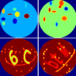
Figure 1: Sample software phantoms randomly generated in order to train the proposed model

II-B Proposed Model

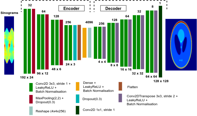
Figure 2: Structure of the proposed model based on deep convolutionl neural networks

Artificial Neural networks and, more specifically, Convolutional neural network (CNN) have been used with great success in multiple domains to analyse visual representations. Initially, CNN’s were inspired by physiological and biological processes, and the connectivity model between neurons compares to the structure of the biological visual cortex [12]. CNN’s are designed and require relatively minimum pre-processing of data compared to other methodologies by employing multilayer perceptrons [13]. This minimum prior knowledge provision provides an essential advantage of CNN’s over other methodologies where prior knowledge and feedback from experts are required. CNN’s have already successfully implemented in medical image analysis [14], and classification [15, 16].

As shown in Figure 2, the proposed model structure consists of two parts, the encoder and the decoder. The encoder consists of five blocks. The first three blocks consist of two convolutional layers with 3x3 kernel and rectified nonlinear activation function (Leaky ReLU) [17], followed by a batch normalisation layer, and a 2x2 max pooling layer [18] and a Dropout layer of 30%. The fourth block consists of two convolutional layers with a 3x3 kernel, a batch normalisation layer, a Leaky ReLU activation function, a Dropout layer of 30% and a flatten layer. The fifth layer consists of a dense layer of 4096 neurons, a Leaky ReLU activation function, and a batch normalisation layer. The number of kernels increases for each block, beginning with 32 kernels for the first block, 64, 128 and 256 for the second, third and fourth blocks, respectively.

Before the data are passed to the decoder, the decoder’s output is transformed from 4096 features to a vector of 4x4x256. The decoder consists of six blocks. The first five blocks consist of two convolutional layers and a transposed convolutional layers, with a stride of 2, with a 3x3 kernel and Leaky ReLU activation function and a batch normalisation layer. The final sixth layer consists of a convolutional layer of 1x1 kernel and linear activation function. The number of kernels decreases for each block, beginning with 256 kernels for the first block, 128, 64, 32, 8 and 1 for the second, third, fourth, fifth and sixth blocks, respectively. Structural Similarity (SSIM) Index [19] was used as the loss function for the training of the proposed method, as shown in equation 1

$$SSIM(x,y)=\frac{(2\mu_{x}\mu_{y}+C_{1})(2\sigma_{xy}+C_{2})}{(\mu_{x}^{2}+\mu_{y}^{2}+C_{1})(\sigma_{x}^{2}+\sigma_{y}^{2}+C_{2})}$$ (1)

where $\mu_{x}$, $\mu_{y}$ and $\sigma_{x}^{2}$, $\sigma_{y}^{2}$ represent the average and variance of $x$ and $y$ respectively while $\sigma_{{xy}}$ represent the covariance of $x$ and $y$; $c_{1}=(k_{1}L)^{2}$, $c_{2}=(k_{2}L)^{2}$ two variables to stabilise the division with weak denominator; $L$ the dynamic range of the pixel-values (typically this is $2^{{\#bits\ per\ pixel}}-1)$; $k_{1}=0.01$ and $k_{2}=0.03$ by default.

III Results and Discussions

The performance of the proposed method was compared against existing methods by using the Mean Square Error (MSE), Structural Similarity (SSIM) Index [19], and the Pearson Correlation Coefficient (PCC) [20]. As the results show and illustrated in Table I, the proposed methodology outperforms MLEM with 0.003 versus 0.006, 0.92 versus 0.77 and 0.96 versus 0.93 for MSE, SSIM and PCC respectively. The proposed method was also tested using hardware phantoms generated using a small FOV SPECT system [21] of three parallel pillars, as shown in Figure 3 with the activity of 21 $\mu Ci$ and variant background activity of 190, 360 and 700 $\mu Ci$. The results are presented in figure 5.

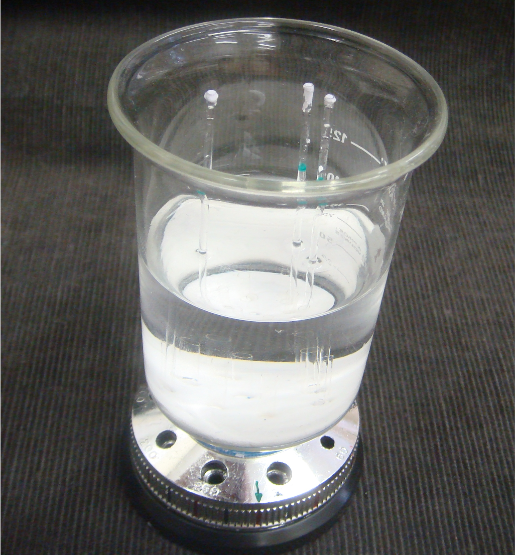
Figure 3: Hardware phantoms of three parallel pillars, with activity of 21 $\mu Ci$ and variant background activity of 190, 360 and 700 $\mu Ci$

TABLE I: Results

Methodology	MSE	SSIM	PCC
MLEM	0.006	0.77	0.93
Proposed Model	0.003	0.92	0.96

(a) True activity of the Shepp Logan Phantom

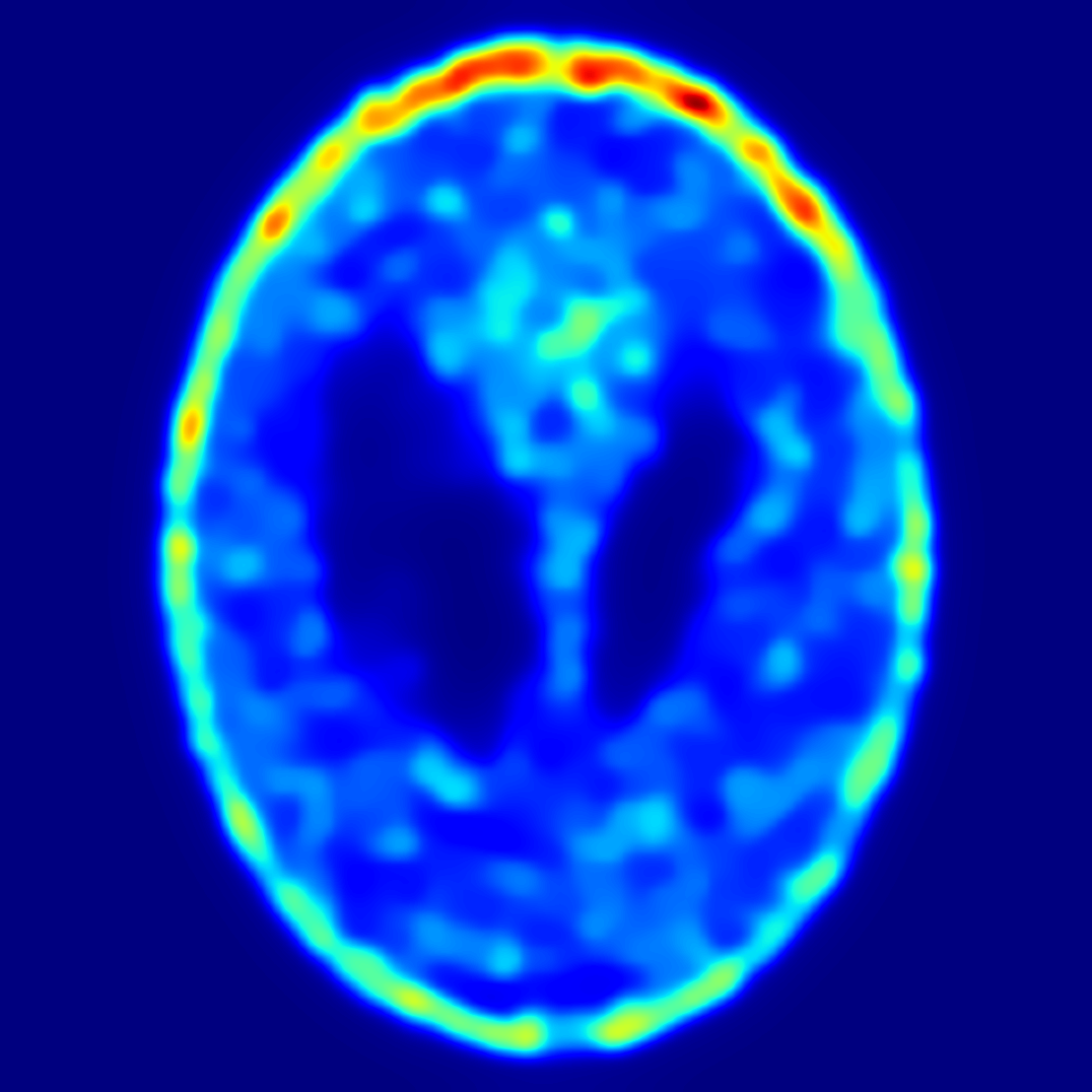
(b) MLEM Reconstruction of the Shepp Logan Phantom

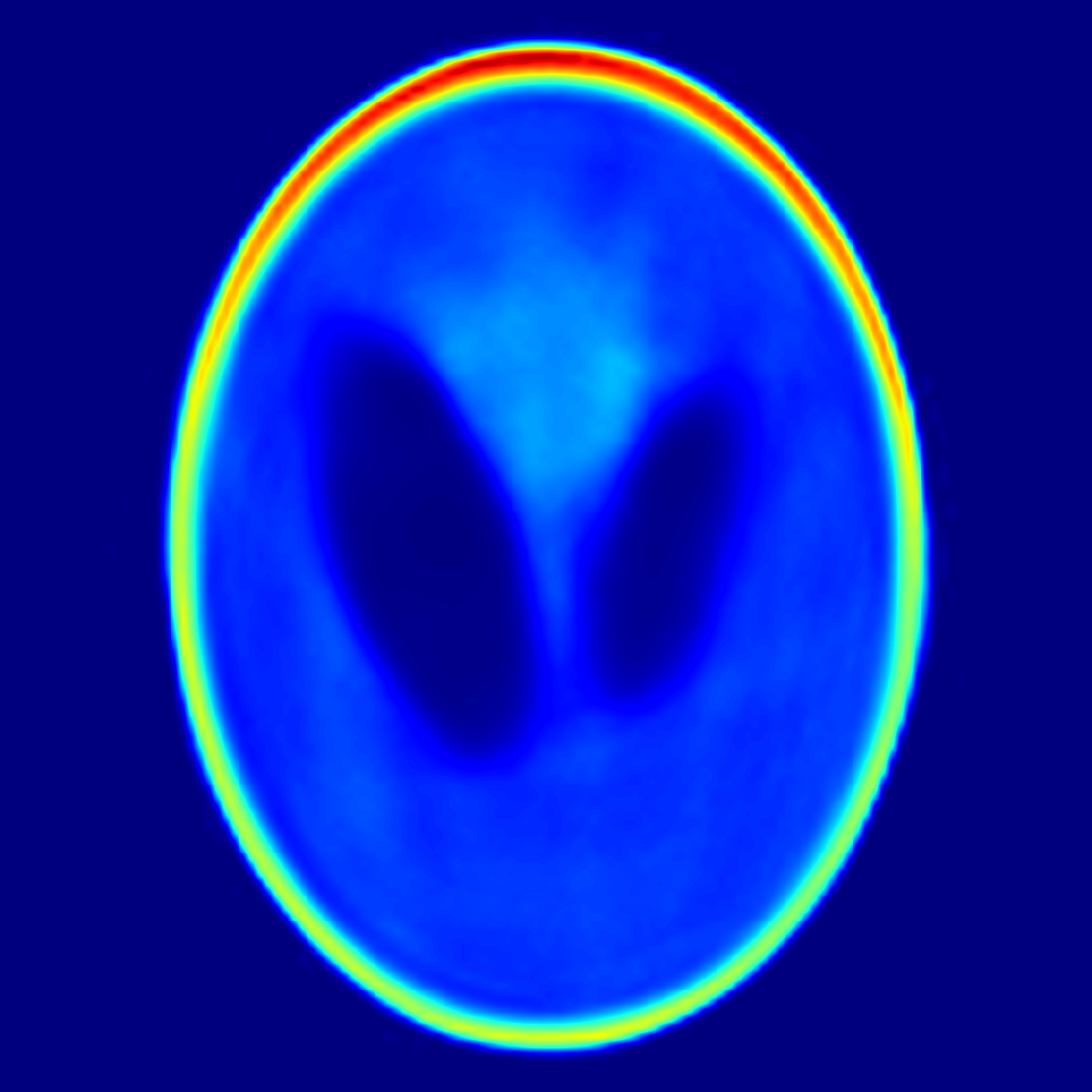
(c) CNNR Reconstruction of the Shepp Logan Phantom

Figure 4: Evaluation of the proposed method results compared to the MLEM method using the Shepp Logan Phantom. The results achieved using the proposed method compare favourably to those obtained with the widely used MLEM method.

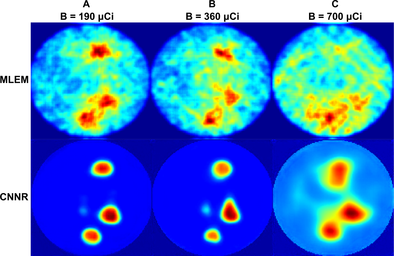
Figure 5: Evaluation of the proposed method results compared to the MLEM method using the Hardware phantoms.

IV Conclusions

In this paper, we proposed a new method based on convolutional neural networks to reconstruct SPECT imaging and demonstrate its capability to reconstruct images with a limited number of projections. As the results show, the proposed method can significantly outperform existing methods such as MLEM. Although the results presented in this proposed work are appropriate for representing the proposed method’s capabilities, further experimentation is needed, as shown in Figure 3 were the size and shape of the reconstructed caterpillars where overestimated.

References

- [1] A. B. De González, M. Mahesh, K.-P. Kim, M. Bhargavan, R. Lewis, F. Mettler, and C. Land, “Projected cancer risks from computed tomographic scans performed in the united states in 2007,” Archives of internal medicine, vol. 169, no. 22, pp. 2071–2077, 2009.
- [2] M. N. Wernick and J. N. Aarsvold, Emission tomography: the fundamentals of PET and SPECT. Elsevier, 2004.
- [3] M. T. Madsen, “Recent advances in spect imaging,” Journal of Nuclear Medicine, vol. 48, no. 4, p. 661, 2007.
- [4] G. Mariani, L. Bruselli, T. Kuwert, E. E. Kim, A. Flotats, O. Israel, M. Dondi, and N. Watanabe, “A review on the clinical uses of spect/ct,” European journal of nuclear medicine and molecular imaging, vol. 37, no. 10, pp. 1959–1985, 2010.
- [5] S. R. Cherry, “Fundamentals of positron emission tomography and applications in preclinical drug development,” The Journal of Clinical Pharmacology, vol. 41, no. 5, pp. 482–491, 2001.
- [6] J. J. Vaquero and P. Kinahan, “Positron emission tomography: current challenges and opportunities for technological advances in clinical and preclinical imaging systems,” Annual review of biomedical engineering, vol. 17, pp. 385–414, 2015.
- [7] M. Perri, P. Erba, D. Volterrani, E. Lazzeri, G. Boni, M. Grosso, and G. Mariani, “Octreo-spect/ct imaging for accurate detection and localization of suspected neuroendocrine tumors,” The Quarterly Journal of Nuclear Medicine and Molecular Imaging, vol. 52, no. 4, p. 323, 2008.
- [8] J. Chen, E. V. Garcia, R. D. Folks, C. D. Cooke, T. L. Faber, E. L. Tauxe, and A. E. Iskandrian, “Onset of left ventricular mechanical contraction as determined by phase analysis of ecg-gated myocardial perfusion spect imaging: development of a diagnostic tool for assessment of cardiac mechanical dyssynchrony,” Journal of nuclear cardiology, vol. 12, no. 6, pp. 687–695, 2005.
- [9] H. M. Hudson and R. S. Larkin, “Accelerated image reconstruction using ordered subsets of projection data,” IEEE transactions on medical imaging, vol. 13, no. 4, pp. 601–609, 1994.
- [10] L. A. Shepp and Y. Vardi, “Maximum likelihood reconstruction for emission tomography,” IEEE transactions on medical imaging, vol. 1, no. 2, pp. 113–122, 1982.
- [11] L. A. Shepp and B. F. Logan, “The fourier reconstruction of a head section,” IEEE Transactions on nuclear science, vol. 21, no. 3, pp. 21–43, 1974.
- [12] D. H. Hubel and T. N. Wiesel, “Receptive fields, binocular interaction and functional architecture in the cat’s visual cortex,” The Journal of physiology, vol. 160, no. 1, pp. 106–154, 1962.
- [13] J. Schmidhuber, “Deep learning in neural networks: An overview,” Neural networks, vol. 61, pp. 85–117, 2015.
- [14] G. Litjens, T. Kooi, B. E. Bejnordi, A. A. A. Setio, F. Ciompi, M. Ghafoorian, J. A. van der Laak, B. van Ginneken, and C. I. Sánchez, “A survey on deep learning in medical image analysis,” Medical image analysis, vol. 42, pp. 60–88, 2017.
- [15] C. Chrysostomou, L. Koutsantonis, C. Lemesios, and C. N. Papanicolas, “A reconstruction method based on deep convolutional neural network for spect imaging,” in 2018 IEEE Nuclear Science Symposium and Medical Imaging Conference Proceedings (NSS/MIC). IEEE, 2018, pp. 1–4.
- [16] ——, “Spect imaging reconstruction method based on deep convolutional neural network,” in 2019 IEEE Nuclear Science Symposium and Medical Imaging Conference (NSS/MIC). IEEE, 2019, pp. 1–4.
- [17] A. L. Maas, A. Y. Hannun, and A. Y. Ng, “Rectifier nonlinearities improve neural network acoustic models,” in Proc. icml, vol. 30, no. 1, 2013, p. 3.
- [18] I. Goodfellow, Y. Bengio, A. Courville, and Y. Bengio, Deep learning. MIT press Cambridge, 2016, vol. 1, no. 2.
- [19] Z. Wang, A. C. Bovik, H. R. Sheikh, and E. P. Simoncelli, “Image quality assessment: from error visibility to structural similarity,” IEEE transactions on image processing, vol. 13, no. 4, pp. 600–612, 2004.
- [20] J. Benesty, J. Chen, Y. Huang, and I. Cohen, “Pearson correlation coefficient,” in Noise reduction in speech processing. Springer, 2009, pp. 1–4.
- [21] V. Spanoudaki, N. Giokaris, A. Karabarbounis, G. Loudos, D. Maintas, C. Papanicolas, P. Paschalis, and E. Stiliaris, “Design and development of a position-sensitive -camera for spect imaging based on pci electronics,” Nuclear Instruments and Methods in Physics Research Section A: Accelerators, Spectrometers, Detectors and Associated Equipment, vol. 527, no. 1-2, pp. 151–156, 2004.