Jeans Instability from post-Newtonian Boltzmann equation

Abstract

Jeans instability within the framework of post-Newtonian Boltzmann and Poisson equations are analyzed. The components of the energy-momentum tensor are calculated from a post-Newtonian Maxwell-Jüttner distribution function. The perturbations of the distribution function and gravitational potentials from their background states with the representation of the perturbations as plane waves lead to a dispersion relation with post-Newtonian corrections. The influence of the post-Newtonian approximation on the Jeans mass is determined and it was shown that the mass necessary for an overdensity to begin the gravitational collapse in the post-Newtonian theory is smaller than the one in the Newtonian theory.

I Introduction

The first attempt to describe instabilities of self-gravitating fluids from the hydrodynamic equations coupled with the Newtonian Poisson equation was due to Jeans [1]. He determined from a dispersion relation a wavelength cutoff, nowadays known as Jeans wavelength, such that for small wavelengths than the Jeans wavelength the perturbations propagate as harmonic waves in time but for large wavelengths the perturbations will grow or decay with time. The gravitational collapse of self-gravitating interstellar gas clouds associated with the mass density perturbations which grow exponentially with time is known as Jeans instability [2, 3, 4]. Physically the collapse of a mass density inhomogeneity occurs whenever the inwards gravitational force is bigger than the outwards pressure force.

Another method to analyse the Jeans instability is to consider the collisionless Boltzmann equation coupled with the Newtonian Poisson equation (see e.g [5, 6, 7, 8, 9, 10, 11, 12]).

Recently the Jeans instability was examined within the framework of the first post-Newtonian theory by considering the hydrodynamic equations and the Poisson equations which follow from this theory [13].

The aim of the present work is to analyse the Jeans instability from the post-Newtonian collisionless Boltzmann equation coupled with the post-Newtonian Poisson equations. Apart from the Newtonian gravitational potential in the first post-Newtonian theory appear two more gravitational potentials which are associated with two new Poisson equations. One of the gravitational potentials is a scalar while the other is a vector [2, 14].

Here the components of the energy-momentum tensor, which appear in the post-Newtonian Poisson equations, are functions of the one-particle distribution function, so that the Poisson equations together with the post-Newtonian Boltzmann equation become a closed system of algebraic equations for the perturbed gravitational potentials. From the solution of the system of algebraic equations a dispersion relation emerges that is used to determine the influence of the post-Newtonian approximation in the Jeans mass, which is related with the minimum mass necessary for an overdensity to initiate the gravitational collapse.

The paper is structured as follows. In Section II the first post-Newtonian expressions for the Boltzmann and Poisson equations and the equilibrium Maxwell-Jüttner distribution function are introduced. The Jeans instability is analyzed in Section III where perturbations in the background states of the distribution function and gravitational potentials are considered. The representation of the perturbations as plane waves results into a dispersion relation where the post-Newtonian influence in the Jeans mass is analyzed. In Section IV a summary of the results is discussed.

II Boltzmann equation

In the first post-Newtonian approximation the components of the metric tensor $g_{\mu\nu}$ reads [14]

$$g_{00}=1-\frac{2U}{c^{2}}+\frac{2}{c^{4}}\left(U^{2}-2\Phi\right),\qquad g_{0i}=\frac{\Pi_{i}}{c^{3}},\qquad g_{ij}=-\left(1+\frac{2U}{c^{2}}\right)\delta_{ij},$$ (1)

where the gravitational potentials $U$, $\Phi$ and $\Pi_{i}$ are given by the Poisson equations

$$\nabla^{2}U=-\frac{4\pi G}{c^{2}}\,{\buildrel\!\!\!\!{}_{0}\over{T^{00}}},\qquad\nabla^{2}\Phi=-2\pi G\left({\buildrel\!\!\!\!{}_{2}\over{T^{00}}}+{\buildrel\!\!\!\!{}_{2}\over{T^{ii}}}\right),$$ (2)

$$\nabla^{2}\Pi^{i}=-\frac{16\pi G}{c}{\buildrel\!\!\!\!{}_{1}\over{T^{0i}}}+\frac{\partial^{2}U}{\partial t\partial x^{i}}.$$ (3)

In the above equations the energy-momentum tensor is split in orders of $1/c^{n}$ denoted by ${\buildrel\!\!\!\!{}_{n}\over{T^{\mu\nu}}}$.

The first post-Newtonian approximation of the Boltzmann equation written in terms of the Chandrasekhar gravitational potentials $U$, $\Phi$ and $\Pi_{i}$ reads

$$\bigg{[}\frac{\partial f}{\partial t}+v_{i}\frac{\partial f}{\partial x^{i}}+\frac{\partial f}{\partial v_{i}}\frac{\partial U}{\partial x^{i}}\bigg{]}\bigg{[}1+\frac{1}{c^{2}}\left(\frac{v^{2}}{2}+U\right)\bigg{]}+\frac{1}{c^{2}}\frac{\partial f}{\partial v_{i}}\bigg{\{}v_{j}\bigg{(}\frac{\partial\Pi_{i}}{\partial x^{j}}-\frac{\partial\Pi_{j}}{\partial x^{i}}\bigg{)}-2v_{i}\frac{\partial U}{\partial t}-2\frac{\partial\left(U^{2}-\Phi\right)}{\partial x^{i}}$$

$$+\frac{\partial\Pi_{i}}{\partial t}-2v_{i}v_{j}\frac{\partial U}{\partial x^{j}}+v^{2}\frac{\partial U}{\partial x^{i}}-v_{i}\bigg{[}\frac{\partial U}{\partial t}+2v_{j}\frac{\partial U}{\partial x^{j}}\bigg{]}\bigg{\}}=0.$$ (4)

In kinetic theory of gases the energy-momentum tensor is defined in terms of the one-particle distribution function by [15]

$$T^{\mu\nu}=m^{4}c\int u^{\mu}u^{\nu}f\frac{\sqrt{-g}\,d^{3}u}{u_{0}}.$$ (5)

Here $u^{\mu}$ is the particle four-velocity whose components in the first post-Newtonian approximation are

$$u^{0}=c\left[1+\frac{1}{c^{2}}\left(\frac{v^{2}}{2}+U\right)\right],\qquad u^{i}=\frac{u^{0}v^{i}}{c}.$$ (6)

The one-particle distribution function at equilibrium for a relativistic gas is given by the Maxwell-Jüttner distribution function. Its expression in the first post-Newtonian approximation in a stationary equilibrium background where the hydrodynamic velocity vanishes is [19]

$$f_{MJ}=f_{0}\left\{1-\frac{\sigma^{2}}{c^{2}}\left[\frac{15}{8}+\frac{3v^{4}}{8\sigma^{4}}+\frac{2Uv^{2}}{\sigma^{4}}\right]\right\},$$ (7)

$$f_{0}=\frac{\rho_{0}}{m^{4}(2\pi\sigma^{2})^{\frac{3}{2}}}e^{-\frac{v^{2}}{2\sigma^{2}}}.$$ (8)

Here $f_{0}$ denotes the Maxwellian distribution function which is given in terms of the gas particle velocity $\bf v$, the mass density $\rho_{0}$ and the dispersion velocity $\sigma=\sqrt{kT_{0}/m}$. Furthermore, $k$ denotes the Boltzmann constant, $T_{0}$ the temperature and $m$ the rest mass of a gas particle. The mass density $\rho_{0}$ and the temperature $T_{0}$ are considered to be constants, since they refer to a stationary equilibrium background. The factor $1/m^{4}$ in the Maxwell-Jüttner distribution function is due to the fact that it is given in terms of the momentum four-vector $p^{\mu}$.

The first post-Newtonian approximation of the invariant integration element of the energy-momentum tensor (5) is given by [19]

$$\frac{\sqrt{-g}\,d^{3}u}{u_{0}}=\left\{1+\frac{1}{c^{2}}\left[2v^{2}+6U\right]\right\}\frac{d^{3}v}{c}.$$ (9)

An equivalent expression for the first post-Newtonian Boltzmann equation (4) is obtained from its multiplication by $[1-({v^{2}}/2+U)/c^{2}]$ and by considering terms up to the $1/c^{2}$ order, yielding

$$\frac{\partial f}{\partial t}+v_{i}\frac{\partial f}{\partial x^{i}}+\frac{\partial U}{\partial x^{i}}\frac{\partial f}{\partial v^{i}}+\frac{1}{c^{2}}\bigg{[}\left(v^{2}-4U\right)\frac{\partial U}{\partial x^{i}}-4v_{i}v_{j}\frac{\partial U}{\partial x^{j}}-3v_{i}\frac{\partial U}{\partial t}+2\frac{\partial\Phi}{\partial x^{i}}+\frac{\partial\Pi_{i}}{\partial t}+v_{j}\left(\frac{\partial\Pi_{i}}{\partial x^{j}}-\frac{\partial\Pi_{j}}{\partial x^{i}}\right)\bigg{]}\frac{\partial f}{\partial v^{i}}=0.$$ (10)

III Jeans instability

For the analysis of Jeans instability we shall rely on the Poisson equations (2) and (3) coupled with the Boltzmann equation (10).

We begin by writing the gravitational potentials and the one-particle distribution function as a sum of background and perturbed terms. The background terms refer to an equilibrium state and are denoted by the subscript zero, while the perturbed terms by the subscript 1. Hence, we write

$$f(\mathbf{x},\mathbf{v},t)=f_{MJ}(\mathbf{x},\mathbf{v},t)+\epsilon f_{1}(\mathbf{x},\mathbf{v},t),$$ (11)

$$U(\mathbf{x},\mathbf{v},t)=U_{0}(\mathbf{x})+\epsilon U_{1}(\mathbf{x},\mathbf{v},t),$$ (12)

$$\Phi(\mathbf{x},\mathbf{v},t)=\Phi_{0}(\mathbf{x})+\epsilon\Phi_{1}(\mathbf{x},\mathbf{v},t),$$ (13)

$$\Pi_{i}(\mathbf{x},\mathbf{v},t)=\Pi_{i}^{0}(\mathbf{x})+\epsilon\Pi_{i}^{1}(\mathbf{x},\mathbf{v},t).$$ (14)

Above we introduced a small parameter $\epsilon$ which controls that only linear terms in this parameter should be considered. Later on this parameter will be set equal to one.

If we introduce the representations (11) – (14) into the Boltzmann equation (10) and equate the terms of the same $\epsilon$-order we obtain the following hierarchy of equations

$$\frac{\partial U_{0}}{\partial x^{i}}\frac{\partial f_{MJ}^{0}}{\partial v^{i}}-\frac{2v^{2}f_{0}}{\sigma^{2}c^{2}}v_{i}\frac{\partial U_{0}}{\partial x^{i}}+\frac{1}{c^{2}}\Bigg{[}\left(v^{2}-4U_{0}\right)\frac{\partial U_{0}}{\partial x^{i}}-4v_{i}v_{j}\frac{\partial U_{0}}{\partial x^{j}}+2\frac{\partial\Phi_{0}}{\partial x^{i}}+v_{j}\left(\frac{\partial\Pi^{0}_{i}}{\partial x^{j}}-\frac{\partial\Pi^{0}_{j}}{\partial x^{i}}\right)\Bigg{]}\frac{\partial f_{0}}{\partial v^{i}}=0,$$ (15)

$$\frac{\partial f_{1}}{\partial t}+v_{i}\frac{\partial f_{1}}{\partial x^{i}}+\frac{\partial U_{1}}{\partial x^{i}}\frac{\partial f_{MJ}^{0}}{\partial v^{i}}-\frac{2v^{2}f_{0}}{\sigma^{2}c^{2}}\left(\frac{\partial U_{1}}{\partial t}+v_{i}\frac{\partial U_{1}}{\partial x^{i}}\right)+\frac{\partial U_{0}}{\partial x^{i}}\frac{\partial f_{1}}{\partial v_{i}}-\frac{4v_{i}U_{1}}{c^{2}\sigma^{2}}\frac{\partial U_{0}}{\partial x^{i}}+\frac{1}{c^{2}}\Bigg{[}\left(v^{2}-4U_{0}\right)\frac{\partial U_{0}}{\partial x^{i}}+2\frac{\partial\Phi_{0}}{\partial x^{i}}$$

$$-4v_{i}v_{j}\frac{\partial U_{0}}{\partial x^{j}}+v_{j}\left(\frac{\partial\Pi^{0}_{i}}{\partial x^{j}}-\frac{\partial\Pi^{0}_{j}}{\partial x^{i}}\right)\Bigg{]}\frac{\partial f_{1}}{\partial v^{i}}+\frac{1}{c^{2}}\Bigg{[}2\frac{\partial\Phi_{1}}{\partial x^{i}}+\frac{\partial\Pi^{1}_{i}}{\partial t}+\left(v^{2}-4U_{0}\right)\frac{\partial U_{1}}{\partial x^{i}}-4v_{i}v_{j}\frac{\partial U_{1}}{\partial x^{j}}-4U_{1}\frac{\partial U_{0}}{\partial x^{i}}$$

$$-3v_{i}\frac{\partial U_{1}}{\partial t}+v_{j}\left(\frac{\partial\Pi^{1}_{i}}{\partial x^{j}}-\frac{\partial\Pi^{1}_{j}}{\partial x^{i}}\right)\Bigg{]}\frac{\partial f_{0}}{\partial v^{i}}=0.\qquad$$ (16)

In the above equations we have written the Maxwell-Jüttner distribution function as

$$f_{MJ}=f_{0}\left\{1-\frac{\sigma^{2}}{c^{2}}\left[\frac{15}{8}+\frac{3v^{4}}{8\sigma^{4}}+2\frac{U_{0}v^{2}}{\sigma^{4}}\right]\right\}-2f_{0}\epsilon\frac{U_{1}v^{2}}{c^{2}\sigma^{2}}=f_{MJ}^{0}-2f_{0}\epsilon\frac{U_{1}v^{2}}{c^{2}\sigma^{2}},$$ (17)

where the background Maxwell-Jüttner distribution function was denoted by $f_{MJ}^{0}$.

We note that the background terms are related with a stationary equilibrium state so that the background equation (15) becomes an identity when the gradients of the gravitational potential backgrounds vanish, i.e., $\nabla U_{0}=0$, $\nabla\Phi_{0}=0$ and $\nabla\Pi_{i}^{0}=0$. By considering that the gravitational potential backgrounds are constants the perturbed Boltzmann equation (16) reduces to

$$\frac{\partial f_{1}}{\partial t}+v_{i}\frac{\partial f_{1}}{\partial x^{i}}+\frac{\partial U_{1}}{\partial x^{i}}\frac{\partial f_{MJ}^{0}}{\partial v^{i}}-\frac{2v^{2}f_{0}}{\sigma^{2}c^{2}}\left(\frac{\partial U_{1}}{\partial t}+v_{i}\frac{\partial U_{1}}{\partial x^{i}}\right)+\frac{1}{c^{2}}\Bigg{[}\left(v^{2}-4U_{0}\right)\frac{\partial U_{1}}{\partial x^{i}}+2\frac{\partial\Phi_{1}}{\partial x^{i}}+\frac{\partial\Pi^{1}_{i}}{\partial t}-3v_{i}\frac{\partial U_{1}}{\partial t}$$

$$-4v_{i}v_{j}\frac{\partial U_{1}}{\partial x^{j}}+v_{j}\left(\frac{\partial\Pi^{1}_{i}}{\partial x^{j}}-\frac{\partial\Pi^{1}_{j}}{\partial x^{i}}\right)\Bigg{]}\frac{\partial f_{0}}{\partial v^{i}}=0.$$ (18)

One can observe from the Poisson equations (2) and (3) that they are not satisfied by the conditions of vanishing background potential gravitational gradients, since the right-hand sides of (2) and (3) are given in terms of the energy-momentum tensor which does not vanish at equilibrium. At this point we assume ”Jeans swindle” (see e.g. [4]) to remove this inconsistency and consider that the Poisson equations are valid only for the perturbed distribution function and gravitational potentials.

We note from the perturbed Boltzmann equation (18) that it is a function of the background value of the Newtonian gravitational potential $U_{0}$ which is a constant. In the analysis of the Jeans instability based on the post-Newtonian hydrodynamic equations [13] it was supposed vanishing values for the background gravitational potentials as a part of the ”Jeans swindle”. Here we shall not adopt this statement and will show that the background Newtonian gravitational potential $U_{0}$ has a prominent role in the determination of Jeans mass.

For the determination of the energy-momentum tensor components (5) we have to write the the four-velocity components (6) and the invariant integration element (9) by taking into account the representation of the Newtonian gravitational potential (12), yielding

$$u^{0}=c\left[1+\frac{1}{c^{2}}\left(\frac{v^{2}}{2}+U_{0}+\epsilon U_{1}\right)\right],\qquad u^{i}=\frac{u^{0}v^{i}}{c},$$ (19)

$$\frac{\sqrt{-g}\,d^{3}u}{u_{0}}=\left\{1+\frac{1}{c^{2}}\left[2v^{2}+6U_{0}+6\epsilon U_{1}\right]\right\}\frac{d^{3}v}{c}.$$ (20)

We multiply the one-particle distribution function (11) together with (17) with the invariant element (20) and get

$$f\frac{\sqrt{-g}\,d^{3}u}{u_{0}}=\left\{1-\frac{\sigma^{2}}{c^{2}}\left[\frac{15}{8}+\frac{3v^{4}}{8\sigma^{4}}+2\frac{U_{0}v^{2}}{\sigma^{4}}-2\frac{v^{2}}{\sigma^{2}}\-6\frac{U_{0}}{\sigma^{2}}\right]\right\}f_{0}\frac{d^{3}v}{c}-\epsilon\frac{U_{1}}{c^{2}}\left(\frac{2v^{2}}{\sigma^{2}}-6\right)f_{0}\frac{d^{3}v}{c}$$

$$+\epsilon\left\{1+\frac{1}{c^{2}}\left[2v^{2}+6U_{0}\right]\right\}f_{1}\frac{d^{3}v}{c}.$$ (21)

Now we can evaluate the energy-momentum tensor components that appear in the right-hand sides of the Poisson equations (2) and (3), by inserting the expressions (19) and (21) into the definition of the energy-momentum tensor (5), resulting

$${\buildrel\!\!\!\!{}_{0}\over{T^{00}}}+{\buildrel\!\!\!\!{}_{2}\over{T^{00}}}=m^{4}c\int u^{0}u^{0}f\frac{\sqrt{-g}\,d^{3}u}{u_{0}}=m^{4}c^{2}\int f_{0}\Bigg{[}1-\frac{\sigma^{2}}{c^{2}}\Bigg{(}\frac{15}{8}+\frac{3v^{4}}{8\sigma^{4}}+\frac{2U_{0}v^{2}}{\sigma^{4}}-\frac{3v^{2}}{\sigma^{2}}-\frac{8U_{0}}{\sigma^{2}}\Bigg{)}\Bigg{]}d^{3}v$$

$$\qquad+\epsilon\,m^{4}c^{2}\int\Bigg{\{}f_{1}\Bigg{[}1+\frac{3v^{2}}{c^{2}}+\frac{8U_{0}}{c^{2}}\Bigg{]}-\Bigg{(}\frac{2v^{2}}{\sigma^{2}}-8\Bigg{)}\frac{f_{0}U_{1}}{c^{2}}\Bigg{\}}d^{3}v,$$ (22)

$${\buildrel\!\!\!\!{}_{2}\over{T^{ij}}}=m^{4}c\int u^{i}u^{j}f\frac{\sqrt{-g}\,d^{3}u}{u_{0}}=m^{4}\int v_{i}v_{j}(f_{0}+\epsilon f_{1})d^{3}v,$$ (23)

$${\buildrel\!\!\!\!{}_{1}\over{T^{0i}}}=m^{4}c\int u^{0}u^{i}f\frac{\sqrt{-g}\,d^{3}u}{u_{0}}=m^{4}c\int v_{i}(f_{0}+\epsilon f_{1})d^{3}v.$$ (24)

By taking into account the expressions (22) – (24) for the energy-momentum tensor components we get that the perturbed Poisson equations (2) and (3) become

$$\nabla^{2}U_{1}=-\frac{4\pi G}{c^{2}}[{\buildrel\!\!\!\!{}_{0}\over{T^{00}}}]_{1}=-4\pi Gm^{4}\int f_{1}d^{3}v,$$ (26)

$$\nabla^{2}\Pi_{1}^{i}=-\frac{16\pi G}{c}[{\buildrel\!\!\!\!{}_{1}\over{T^{0i}}}]_{1}+\frac{\partial^{2}U_{1}}{\partial t\partial x^{i}}=-16\pi Gm^{4}\int v_{i}f_{1}d^{3}v+\frac{\partial^{2}U_{1}}{\partial t\partial x^{i}},$$

$$\nabla^{2}\Phi_{1}=-2\pi G\left([{\buildrel\!\!\!\!{}_{2}\over{T^{00}}}]_{1}+[{\buildrel\!\!\!\!{}_{2}\over{T^{ii}}}]_{1}\right)=-2\pi Gm^{4}\int\bigg{[}\left(4v^{2}+8U_{0}\right)f_{1}-\left(\frac{2v^{2}}{\sigma^{2}}-8\right)U_{1}f_{0}\bigg{]}d^{3}v.$$ (27)

In the above equations the energy-momentum tensor components calculated with the perturbed distribution function $f_{1}$ were denoted by $[{\buildrel\!\!\!\!{}_{0}\over{T^{00}}}]_{1}$, $[{\buildrel\!\!\!\!{}_{1}\over{T^{0i}}}]_{1}$ and so one.

As usual for the search of the instabilities the perturbations are represented as plane waves of frequency $\omega$ and wave number vector $\mathbf{k}$, namely

$$f_{1}(\mathbf{x},\mathbf{v},t)=\overline{f}_{1}e^{i(\mathbf{k}\cdot\mathbf{x}-\omega t)},\quad U_{1}(\mathbf{x},\mathbf{v},t)=\overline{U}_{1}e^{i(\mathbf{k}\cdot\mathbf{x}-\omega t)},$$ (28)

$$\Phi_{1}(\mathbf{x},\mathbf{v},t)=\overline{\Phi}_{1}e^{i(\mathbf{k}\cdot\mathbf{x}-\omega t)},\quad\Pi^{i}_{1}(\mathbf{x},\mathbf{v},t)=\overline{\Pi_{i}^{1}}e^{i(\mathbf{k}\cdot\mathbf{x}-\omega t)},$$ (29)

where $\overline{f}_{1},\overline{U}_{1},\overline{\Phi}_{1}$ and $\overline{\Pi_{1}^{i}}$ represent small amplitudes of the perturbations.

If we insert the plane wave representations (28) and (29) into the perturbed Boltzmann equation (18) we get

$$({\bf v\cdot k}-\omega)\overline{f}_{1}-\frac{f_{0}}{\sigma^{2}}\bigg{\{}({\bf v\cdot k})\overline{U}_{1}\bigg{[}1-\frac{\sigma^{2}}{c^{2}}\bigg{(}\frac{15}{8}+\frac{3v^{4}}{8\sigma^{4}}-\frac{v^{2}}{2\sigma^{2}}+\frac{2v^{2}U_{0}}{\sigma^{4}}\bigg{)}\bigg{]}+\frac{1}{c^{2}}\left[v^{2}\omega\overline{U}_{1}+2({\bf v\cdot k})\overline{\Phi}_{1}-\omega v_{i}\overline{\Pi^{1}_{i}}\right]\bigg{\}}=0,$$

(30)

by taking into account the expression (17) for the determination of the term $\partial f_{MJ}/\partial v^{i}$.

The Poisson equations (26) – (27) with the plane wave representations (28) and (29) become

$$\kappa^{2}\overline{U}_{1}=4\pi Gm^{4}\int\overline{f}_{1}d^{3}v,$$ (33)

$$\kappa^{2}\overline{\Pi^{1}_{i}}=16\pi Gm^{4}\int v_{i}\overline{f}_{1}d^{3}v+k_{i}\omega\overline{U}_{1},$$

$$\kappa^{2}\overline{\Phi}_{1}=8\pi Gm^{4}\int(v^{2}+2U_{0})\overline{f}_{1}d^{3}v+4\pi G\rho_{0}\overline{U}_{1}.$$

We have to evaluate the integrals in (33) – (33) and for that end we choose, without loss of generality, the wave number vector in the $x$-direction, i.e., ${\bf k}=(\kappa,0,0)$. We begin with the substitution of $\overline{f}_{1}$ from (30) into (33) and get

$$\kappa^{2}\overline{\Pi^{1}_{i}}=\frac{16\pi G\rho_{0}}{(2\pi\sigma^{2})^{\frac{3}{2}}}\int\frac{v_{i}(v_{x}\kappa+\omega)e^{-\frac{v^{2}}{2\sigma^{2}}}d^{3}v}{\sigma^{2}[(v_{x}\kappa)^{2}-\omega^{2}]}\bigg{\{}v_{x}\kappa\bigg{[}1-\frac{\sigma^{2}}{c^{2}}\bigg{(}\frac{15}{8}+\frac{3v^{4}}{8\sigma^{4}}-\frac{v^{2}}{2\sigma^{2}}+\frac{2U_{0}v^{2}}{\sigma^{4}}\bigg{)}\bigg{]}\overline{U}_{1}$$

$$+\frac{1}{c^{2}}\bigg{[}v^{2}\omega\overline{U}_{1}+2v_{x}\kappa\overline{\Phi}_{1}-\omega v_{j}\overline{\Pi^{1}_{j}}\bigg{]}\bigg{\}}+k_{i}\omega\overline{U}_{1}.$$ (34)

Here the numerator and denominator of the integrand were multiplied by $(v_{x}\kappa+\omega)$.

For the components $i=y,z$ the integration of (34) in the ranges $-\infty<(v_{x},v_{y},v_{z})<\infty$ leads to

$$\kappa^{2}\overline{\Pi^{1}_{i}}=-8\pi G\rho_{0}\frac{\omega^{2}}{\kappa^{2}\sigma^{2}c^{2}}I_{0}\overline{\Pi^{1}_{i}},\qquad i=y,z,$$ (35)

where $I_{0}$ is an integral which is given in terms of the $I_{n}$ integrals defined by

$$I_{n}(\kappa,\omega)=\frac{2}{\sqrt{\pi}}\int_{0}^{\infty}\frac{x^{n}e^{-x^{2}}}{x^{2}-(\omega/\sqrt{2}\sigma\kappa)^{2}}dx,\quad x=\frac{v_{x}}{\sqrt{2}\sigma}.$$ (36)

We conclude from (35) that $\overline{\Pi^{1}_{y}}=\overline{\Pi^{1}_{z}}=0$.

For the component $i=x$ the integration of (34) in the ranges $-\infty<(v_{x},v_{y},v_{z})<\infty$, yields

$$\kappa^{2}\overline{\Pi_{x}^{1}}=\kappa\omega\overline{U}_{1}+\frac{16\pi G\rho_{0}\omega}{\kappa\sigma^{2}}\bigg{\{}\bigg{[}I_{2}-\frac{3\sigma^{2}}{2c^{2}}\left(I_{6}+\frac{5}{4}I_{2}\right)-\frac{4U_{0}}{c^{2}}\left(I_{2}+I_{4}\right)\bigg{]}\overline{U}_{1}+\frac{I_{2}}{c^{2}}\left[2\overline{\Phi}_{1}-\frac{\omega}{\kappa}\overline{\Pi_{x}^{1}}\bigg{]}\right\}.$$ (37)

Now we follow the same methodology and substitute $\overline{f}_{1}$ from (30) into (33) and (33). The subsequent integration of the resulting equations in the ranges $-\infty<(v_{x},v_{y},v_{z})<\infty$ lead to

$$\kappa^{2}\overline{U}_{1}=\frac{4\pi G\rho_{0}}{\sigma^{2}}\bigg{\{}\bigg{[}I_{2}+\left(I_{0}+I_{2}\right)\frac{\omega^{2}}{c^{2}\kappa^{2}}-\frac{3\sigma^{2}}{2c^{2}}\bigg{(}I_{6}+\frac{4}{3}I_{4}+\frac{31}{12}I_{2}\bigg{)}-\frac{4U_{0}}{c^{2}}\left(I_{2}+I_{4}\right)\bigg{]}\overline{U}_{1}+\frac{I_{2}}{c^{2}}\bigg{[}2\overline{\Phi}_{1}-\frac{\omega}{\kappa}\overline{\Pi_{x}^{1}}\bigg{]}\bigg{\}},\quad$$ (38)

$$\kappa^{2}\overline{\Phi}_{1}=4\pi G\rho_{0}\overline{U}_{1}+16\pi G\rho_{0}\bigg{\{}2\bigg{(}I_{0}+I_{2}+\frac{I_{4}}{2}\bigg{)}\frac{\omega^{2}}{\kappa^{2}c^{2}}+I_{2}+I_{4}-\frac{3\sigma^{2}}{2c^{2}}\bigg{(}I_{8}+\frac{7}{3}I_{6}+\frac{71}{12}I_{4}+\frac{71}{12}I_{2}\bigg{)}+\frac{U_{0}}{\sigma^{2}}\bigg{[}I_{2}$$

$$-\frac{\sigma^{2}}{c^{2}}\bigg{(}\frac{11}{2}I_{6}+10I_{4}+\frac{95}{8}I_{2}\bigg{)}-\frac{4U_{0}}{c^{2}}(I_{2}+I_{4})+\frac{\omega^{2}}{c^{2}\kappa^{2}}(I_{0}+I_{2})\bigg{]}\bigg{\}}\overline{U}_{1}+\frac{16\pi G\rho_{0}}{c^{2}}\left(I_{2}+I_{4}+I_{2}\frac{U_{0}}{\sigma^{2}}\right)\left[2\overline{\Phi}_{1}-\frac{\omega}{\kappa}\overline{\Pi_{x}^{1}}\right].\quad$$ (39)

By inspecting equations (37) – (39) we conclude that they represent an algebraic system of equations for the amplitudes $\overline{\Pi_{x}^{1}}$, $\overline{U}_{1}$ and $\overline{\Phi}_{1}$. This system of equations admits a solution if the determinant of the coefficients of $\overline{\Pi_{x}^{1}}$, $\overline{U}_{1}$ and $\overline{\Phi}_{1}$ vanishes. Hence we get the following dispersion relation

$$\kappa_{*}^{4}-\kappa_{*}^{2}\left[I_{2}+\frac{\sigma^{2}}{c^{2}}\left(\frac{33}{8}I_{2}+6I_{4}-\frac{3}{2}I_{6}+4(I_{2}-I_{4})\frac{U_{0}}{\sigma^{2}}\right)\right]-\frac{\sigma^{2}}{c^{2}}\Bigg{[}2I_{2}+\left(I_{0}-4I_{2}\right)\omega_{*}^{2}\Bigg{]}=0.$$ (40)

The above dispersion relation is an algebraic equation which relates the dimensionless wave number $\kappa_{*}$ with the dimensionless frequency $\omega_{*}$. They are defined by

$$\kappa_{*}=\frac{\kappa}{\kappa_{J}},\qquad\omega_{*}=\frac{\omega}{\sqrt{4\pi G\rho_{0}}},$$ (41)

where $\kappa_{J}=\sqrt{4\pi G\rho_{0}}/\sigma$ denotes the Jeans wave number.

Note that in the dispersion relation (40) we have not considered the terms that have order higher than $1/c^{2}$, due to the fact that we are considering only the first post-Newtonian approximation.

The perturbations will propagate as harmonic waves in time if the frequency $\omega$ has real values, while for pure imaginary values of the frequency the perturbation will grow or decay in time. The one which grows with time is associated with the Jeans instability. Hence, the corresponding solutions to the Jeans instability are those where $\omega_{*}=i\omega_{I}$, i.e., $\Re(\omega_{*})=0$ and $\omega_{I}=\Im(\omega_{*})>0$. The integrals (36) in this case can be evaluated, yielding

$$I_{0}=\frac{\kappa_{*}}{\omega_{I}}\sqrt{2\pi}\exp\left(\frac{\omega_{I}^{2}}{2\kappa_{*}^{2}}\right){\rm erfc}\left(\frac{\omega_{I}}{\sqrt{2}\kappa_{*}}\right),\quad I_{2}=1-\frac{\omega_{I}^{2}}{2\kappa_{*}^{2}}I_{0},\quad I_{4}=\frac{1}{2}-\frac{\omega_{I}^{2}}{2\kappa_{*}^{2}}I_{2},\quad I_{6}=\frac{3}{4}-\frac{\omega_{I}^{2}}{2\kappa_{*}^{2}}I_{4}.$$ (42)

Here $\rm{erfc}(x)$ is the complementary error function

$$\rm{erfc}(x)=\frac{2}{\sqrt{\pi}}\int_{x}^{\infty}e^{-x^{2}}dx.$$ (43)

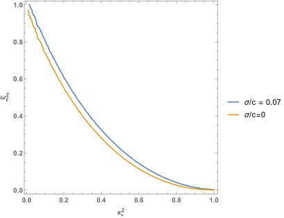
Figure 1: Dimensionless frequency as function of the dimensionless wave number vector modulus for the post-Newtonian ($\sigma/c=0.07$) and Newtonian ($\sigma/c=0$) theories.

The contour plots which follow from the dispersion relation (40) are shown in Figure 1 for two different values of the ratio between the dispersion velocity and the light speed, namely $\sigma/c=0$ which corresponds to the Newtonian theory and $\sigma/c=0.07$ to the post-Newtonian theory. For the evaluation of (40) it was assumed that $U_{0}\approx\sigma^{2}$, which can be justified by the virial theorem where the square of the dispersion velocity can be approximated with the Newtonian gravitational potential. We observe from this figure that the limit of instability in the post-Newtonian theory differs from the one of the Newtonian theory. Indeed, the modulus of the wave number vector for a given frequency in the Newtonian theory is smaller than that of the post-Newtonian theory. As a consequence, the mass limit of interstellar gas clouds necessary to start the gravitational collapse in the post-Newtonian theory is smaller than the one in the Newtonian theory.

Let us investigate the limiting value of the frequency where the instability occurs and which corresponds to the minimum mass where an overdensity begins the gravitational collapse. For that end we set $\omega_{I}=0$ in (40), yielding

$$\kappa_{*}^{4}-\left[1+\frac{\sigma^{2}}{c^{2}}\left(6+\frac{2U_{0}}{\sigma^{2}}+\frac{2}{\kappa_{*}^{2}}\right)\right]\kappa_{*}^{2}=0.$$ (44)

The solution of the fourth order algebraic equation (44) is

$$\kappa_{*}=\pm\sqrt{\frac{1}{2}+\frac{\sigma^{2}}{c^{2}}\left[3+\frac{U_{0}}{\sigma^{2}}\pm\sqrt{\frac{1}{4}+\frac{\sigma^{2}}{c^{2}}\left[5+\frac{U_{0}}{\sigma^{2}}+\frac{\sigma^{2}}{c^{2}}\left(9+\frac{6U_{0}}{\sigma^{2}}+\frac{U_{0}^{2}}{\sigma^{4}}\right)\right]}\right]}$$ (45)

The real positive value of $\kappa_{*}$ when terms up to the $1/c^{2}$ order are considered reads

$$\kappa_{*}=1+\frac{\sigma^{2}}{c^{2}}\left[4+\frac{U_{0}}{\sigma^{2}}\right].$$ (46)

Here we shall call attention to the fact that the post-Newtonian correction is given in terms of the ratio of the dispersion velocity $\sigma$ and the light speed $c$. In a phenomenological theory this correction is given in terms of the adiabatic sound speed $c_{s}$ and the light speed $c$. This difference comes out that the Maxwellian distribution function is written in terms of the dispersion velocity while in the phenomenological theory an adiabatic solution is considered.

In a recent paper Noh and Hwang [20] obtained from a dispersion relation the post-Newtonian correction which corresponds to (46). In our notation the real root of equation (78) of [20] in the post-Newtonian approximation reads

$$\kappa_{*}=1+\frac{c_{s}^{2}}{c^{2}}\left[\frac{\left(\Pi_{0}+\frac{p_{0}}{\rho_{0}}\right)}{c_{s}^{2}}+\frac{5}{2}+\frac{U_{0}}{c_{s}^{2}}\right].$$ (47)

Here $\Pi_{0}=(p_{0}/\rho_{0})/(\gamma-1)$ is the specific internal energy. By considering the adiabatic sound velocity $c_{s}^{2}=\gamma p_{0}/\rho_{0}$ and $\gamma=5/3$ the above equation reduces to

$$\kappa_{*}=1+\frac{c_{s}^{2}}{c^{2}}\left[4+\frac{U_{0}}{c_{s}^{2}}\right],$$ (48)

which has the same structure as (46). This result from a phenomenological theory is the same as the one found in [21].

The Jeans mass is related with the minimum amount of mass for an overdensity to initiate the gravitational collapse and refers to the mass contained in a sphere of radius equal to the wavelength of the perturbation. If we denote the mass corresponding to the post-Newtonian wavelength by $M_{J}^{PN}$ and the Newtonian one by $M_{J}^{N}$ wavelengths, their ratio is given by

$$\frac{M_{J}^{PN}}{M_{J}^{N}}=\frac{\lambda^{3}}{\lambda_{J}^{3}}=\frac{\kappa_{J}^{3}}{\kappa_{*}^{3}}\approx 1-3\frac{\sigma^{2}}{c^{2}}\left[4+\frac{U_{0}}{\sigma^{2}}\right].$$ (49)

From the above equation we infer that in the post-Newtonian framework the mass needed to begin the gravitational collapse is smaller than in the Newtonian one. Furthermore, we note that the background Newtonian potential has an important role, since it implies a smaller mass than the one without it. As was previously commented one can make use of the virial theorem to approximate $U_{0}\approx\sigma^{2}$, so that (50) becomes

$$\frac{M_{J}^{PN}}{M_{J}^{N}}=1-15\frac{\sigma^{2}}{c^{2}}.$$ (50)

IV Summary

In this work the Jeans instability was analysed within the framework of the Boltzmann and Poisson equations that follow from the first post-Newtonian theory. The components of the energy-momentum tensor in the Poisson equations were determined from the Maxwell-Jüttner distribution function. The distribution function and the gravitational potentials were perturbed from their background states and a plane wave representation for the perturbations was considered. The post-Newtonian dispersion relation was obtained from an algebraic system of equations for the perturbed gravitational potentials. It was shown that the mass necessary for an overdensity to begin the gravitational collapse in the post-Newtonian theory is smaller than the one in the Newtonian one. Furthermore, a non-vanishing Newtonian gravitational potential background implies a smaller Jeans mass than the one where a vanishing value is considered [13].

References

• [1] J. H. Jeans, Philos. Trans. R. Soc. A 199, 1 (1902)
• [2] S. Weinberg, Gravitation and cosmology. Principles and applications of the theory of relativity (Wiley, New York, 1972).
• [3] P. Coles and F. Lucchin, Cosmology. The Origin and Evolution of Cosmic structures, 2nd, edn. ( John Wiley, Chichester, 2002).
• [4] J. Binney and S. Tremaine Galactic Dynamics, 2nd. edn. (Princeton University Press, Princeton, 2008).
• [5] S. A. Trigger, A. I. Ershkovich, G. J. F. van Heijst and P. P. J. M. Schram, Phys. Rev. E 69, 066403 (2004)
• [6] S. Capozziello, M. De Laurentis, I. De Martino, M. Formisano and S. D. Odintsov, Phys. Rev. D 85, 044022 (2012)
• [7] S. Capozziello and M. De Laurentis, Ann. Phys. 524, 545 (2012)
• [8] G. M. Kremer and R. André, Int. J. Mod. Phys. D 25, 1650012 (2016)
• [9] G. M. Kremer, AIP Conference Proceedings 1786, 160002 (2016)
• [10] I. De Martino and A. Capolupo, Eur. Phys. J. C 77, 715 (2017)
• [11] G. M. Kremer, M. G. Richarte and E. M. Schiefer, Eur. Phys. J. C 79, 492 (2019)
• [12] G. M. Kremer, Physica A 545, 123667 (2020)
• [13] E. Nazari, A. Kazemi, M. Roshan and S. Abbassi, Ap. J. 839, 839 (2017)
• [14] S. Chandrasekhar, Ap. J. 142, 1488 (1965)
• [15] C. Cercignani and G. M. Kremer, The relativistic Boltzmann equation: theory and applications (Birkhäuser, Basel, 2002).
• [16] V. Rezania and Y. Sobouti, Astron. Astrophys. 354, 1110 (2000)
• [17] C. A. Agón, J. F. Pedraza and J. Ramos-Caro, Phys. Rev. D 83, 123007 (2011)
• [18] G.M. Kremer, Annals of Physics 426, 168400 (2021)
• [19] G. M. Kremer, M. G. Richarte and K. Weber, Phys. Rev. D 93, 064073 (2016)
• [20] H. Noh and J-C Hwang, ApJ, 906, 22 (2021).
• [21] G. M. Kremer, Post-Newtonian hydrodynamics: theory and applications, to be published by Cambridge Scholars Publishing, 2021.