FZZT branes in JT gravity and topological gravity

Abstract

We study Fateev-Zamolodchikov-Zamolodchikov-Teschner (FZZT) branes in Witten-Kontsevich topological gravity, which includes Jackiw-Teitelboim (JT) gravity as a special case. Adding FZZT branes to topological gravity corresponds to inserting determinant operators in the dual matrix integral and amounts to a certain shift of the infinitely many couplings of topological gravity. We clarify the perturbative interpretation of adding FZZT branes in the genus expansion of topological gravity in terms of a simple boundary factor and the generalized Weil-Petersson volumes. As a concrete illustration we study JT gravity in the presence of FZZT branes and discuss its relation to the deformations of the dilaton potential that give rise to conical defects. We then construct a non-perturbative formulation of FZZT branes and derive a closed expression for the general correlation function of multiple FZZT branes and multiple macroscopic loops. As an application we study the FZZT-macroscopic loop correlators in the Airy case. We observe numerically a void in the eigenvalue density due to the eigenvalue repulsion induced by FZZT-branes and also the oscillatory behavior of the spectral form factor which is expected from the picture of eigenbranes.

1 Introduction

Two-dimensional Jackiw-Teitelboim (JT) gravity Jackiw:1984je ; Teitelboim:1983ux is a useful toy model to study various aspects of quantum gravity and holography. In a remarkable paper Saad:2019lba it was shown that JT gravity is holographically dual to a certain double-scaled matrix model. This is an example of the holography involving the ensemble average, where the Hamiltonian $H$ of the boundary theory becomes the random matrix. This in particular implies that the correlator of two partition functions $\langle Z(\beta_{1})Z(\beta_{2})\rangle$ includes the contribution of spacetime wormhole connecting the two asymptotic boundaries and thus the correlator is not factorized.

As argued in Blommaert:2019wfy , one can fix some of the eigenvalues of the matrix integral by introducing the Fateev-Zamolodchikov-Zamolodchikov-Teschner (FZZT) branes Fateev:2000ik ; Teschner:2000md , which are called “eigenbranes” in Blommaert:2019wfy . Adding branes in JT gravity is also considered in Penington:2019kki to recover the Page curve for black hole evaporation. In a recent paper Gao:2021uro , the matrix model for the dynamical end of the world (EOW) brane in JT gravity is proposed.

In this paper, we consider FZZT branes in JT gravity. Our prescription for introducing the FZZT branes is a natural generalization of the JT gravity matrix model by Saad, Shenker and Stanford Saad:2019lba . We obtain the amplitude in the presence of FZZT branes by gluing several building blocks. As shown in Saad:2019lba , the JT gravity amplitude is obtained by gluing the “trumpet” (9) and the Weil-Petersson (WP) volume (6). A new ingredient in the presence of a FZZT brane is the factor $\mathcal{M}(b)=-e^{-zb}$ with $z$ being a parameter, which is attached to the geodesic boundary of length $b$ and we integrate over $b$ (see Figure 1). This construction can be generalized to multiple FZZT branes by replacing the factor with $\mathcal{M}(b)=-\sum_{i}e^{-z_{i}b}$. In particular, the trumpet can end on a FZZT brane as shown in Figure 1(a). This implies that the two-boundary correlator $\langle Z(\beta_{1})Z(\beta_{2})\rangle$ in the presence of FZZT brane receives a contribution depicted in Figure 2(b), which reminds us of the “half-wormhole” introduced in Saad:2021rcu .

(a) Trumpet ending on a FZZT brane

(b) Higher genus correction

Figure 1: Trumpet can end on a FZZT brane. We attach the factor $\mathcal{M}(b)=-e^{-zb}$ to the geodesic boundary and integrate over $b$.

(a) Wormhole

(b) Half-wormholes

Figure 2: Contributions of 2(a) wormhole and 2(b) half-wormholes.

It turns out that the above construction of FZZT branes in JT gravity can be generalized to encompass arbitrary background $\{t_{k}\}$ of 2d topological gravity. We can compute FZZT brane amplitude by gluing certain building blocks. In general background $\{t_{k}\}$, we can use the same “trumpet” and $\mathcal{M}(b)$ as in JT gravity, but the WP volume should be replaced by the generalized WP volume defined in (37).

This construction defines an FZZT brane amplitude only perturbatively in genus expansion. One can obtain the non-perturbative expression of the correlator of FZZT branes and macroscopic loop operators $Z(\beta)=\operatorname{Tr}e^{-\beta H}$ by taking a double scaling limit of the correlator of determinants in the finite $N$ matrix model. We find a compact expression of the generating function of the $Z(\beta)$-FZZT correlators in terms of the Baker-Akhiezer (BA) function and the Christoffel-Darboux (CD) kernel (see (203) and (204)). As an application of our formalism, we consider the spectral form factor in the presence of two FZZT branes (see Figure 6).

This paper is organized as follows. In section 2, we find the prescription for the construction of FZZT brane amplitude by gluing the trumpet, (generalized) WP volume and $\mathcal{M}(b)$. We find that the half-wormhole amplitude is given by the complementary error function (57). We also comment on the relation between the trumpet and the Liouville wavefunction. In section 3, we compute the genus-zero density of states in JT gravity with $K$ FZZT branes in the ’t Hooft limit (80). We also comment on the relation to the deformation of the potential of dilaton gravity. In section 4, we review the known results about the BA function, the CD kernel and the multi-FZZT amplitude. In section 5, we find the generating functions (203) and (204) of the correlators of FZZT branes and macroscopic loop operators. In section 6, we apply our formalism to the Airy case, i.e. the trivial background $t_{k}=0~{}(k\geq 1)$ of topological gravity. We study the spectral form factor in the presence of two FZZT branes in the Airy case. Finally we conclude in section 7. In appendix A we summarize the result of $(2,p)$ minimal string. In appendix B we provide an alternative derivation of (176) using the correlator of inverse determinant.

2 FZZT branes in the genus expansion

In this section, we will explain our formalism of computing the genus expansion of the correlator of partition functions $Z(\beta)=\operatorname{Tr}e^{-\beta H}$ in the presence of FZZT branes.

2.1 JT gravity and Weil-Petersson volume

Let us first consider JT gravity. As shown by Saad, Shenker and Stanford Saad:2019lba , the genus expansion of the connected correlator of $Z(\beta)$’s can be obtained by gluing the “trumpet” and the Weil-Petersson (WP) volume

$$\left\langle\prod_{i=1}^{n}Z(\beta_{i})\right\rangle_{\rm c}=\sum_{g=0}^{\infty}e^{-(2g-2+n)S_{0}}\prod_{i=1}^{n}\int_{0}^{\infty}\tilde{b}_{i}d\tilde{b}_{i}\tilde{Z}_{\text{trumpet}}(\beta,\tilde{b}_{i})\tilde{V}_{g,n}(\tilde{b}_{1},\ldots,\tilde{b}_{n}),$$ (1)

where the subscript ${\rm c}$ of $\langle\cdots\rangle_{\rm c}$ refers to the connected part. The WP volume $\tilde{V}_{g,n}(\bm{\tilde{b}})$ is given by

$$\tilde{V}_{g,n}(\bm{\tilde{b}}) =\int_{\overline{\mathcal{M}}_{g,n}}e^{2\pi^{2}\kappa+\frac{1}{2}\sum_{i=1}^{n}\tilde{b}_{i}^{2}\psi_{i}},$$ (2)

where $\overline{\cal M}_{g,n}$ denotes the Deligne-Mumford compactification of the moduli space of ${\cal M}_{g,n}$ of Riemann surface $\Sigma$ of genus $g$ with $n$ marked points $p_{1},\ldots,p_{n}$, $\kappa$ is the first Miller-Morita-Mumford class and $\psi_{i}$ is the first Chern class of the complex line bundle whose fiber is the cotangent space to $p_{i}$. Note that (2) is valid for $3g-3+n\geq 0$ and $\tilde{V}_{0,1},\tilde{V}_{0,2}$ are undefined. Correspondingly, (1) makes sense except the contributions of the disk and annulus amplitudes, which are to be discussed separately. The trumpet partition function $\tilde{Z}_{\text{trumpet}}(\beta,\tilde{b})$ in (1) is given by

$$\tilde{Z}_{\text{trumpet}}(\beta,\tilde{b})=\frac{\sqrt{\gamma}}{\sqrt{2\pi\beta}}e^{-\frac{\gamma\tilde{b}^{2}}{2\beta}},$$ (3)

where $\gamma$ is the asymptotic value of the dilaton field near the boundary of $AdS_{2}$.

It is convenient to set

$$\gamma=\frac{1}{2\pi^{2}},\quad\tilde{b}^{2}=2\pi^{2}b^{2}.$$ (4)

Then we find

$$\tilde{V}_{g,n}(\bm{\tilde{b}}) =\int_{\overline{\mathcal{M}}_{g,n}}e^{2\pi^{2}(\kappa+\frac{1}{2}\sum_{i}b_{i}^{2}\psi_{i})}=(2\pi^{2})^{3g-3+n}V_{g,n}(\bm{b}),$$ (5)

where we defined the rescaled WP volume by

$$V_{g,n}(\bm{b})=\int_{\overline{\mathcal{M}}_{g,n}}e^{\kappa+\frac{1}{2}\sum_{i=1}^{n}b_{i}^{2}\psi_{i}}.$$ (6)

In what follows we will call $V_{g,n}(\bm{b})$ the WP volume instead of the original $\tilde{V}_{g,n}(\bm{\tilde{b}})$. As in our previous paper Okuyama:2019xbv we define the genus counting parameter $g_{\rm s}$ by

$$g_{\rm s}=(2\pi^{2})^{\frac{3}{2}}e^{-S_{0}}.$$ (7)

It is also convenient to rescale the trumpet so that

$$e^{-S_{0}(2g-2+n)}\tilde{V}_{g,n}(\bm{\tilde{b}})\prod_{i=1}^{n}\tilde{b}_{i}d\tilde{b}_{i}\tilde{Z}_{\text{trumpet}}(\beta,\tilde{b}_{i})=g_{\rm s}^{2g-2+n}V_{g,n}(\bm{b})\prod_{i=1}^{n}b_{i}db_{i}Z_{\text{trumpet}}(\beta,b_{i}).$$ (8)

Then we find

$$Z_{\text{trumpet}}(\beta,b)=\frac{e^{-\frac{b^{2}}{2\beta}}}{\sqrt{2\pi\beta}}.$$ (9)

In this new normalization, (1) is written as

$$\left\langle\prod_{i=1}^{n}Z(\beta_{i})\right\rangle_{\rm c}=\sum_{g=0}^{\infty}g_{\rm s}^{2g-2+n}\prod_{i=1}^{n}\int_{0}^{\infty}b_{i}db_{i}Z_{\text{trumpet}}(\beta,b_{i})V_{g,n}(\bm{b}).$$ (10)

Now let us consider the effect of adding FZZT branes. In the matrix model the FZZT brane corresponds to the insertion of the determinant operator $\det(\xi+H)$ in the matrix integral, where $H$ is the matrix variable and $\xi$ is a formal parameter Kutasov:2004fg ; Maldacena:2004sn . The FZZT brane operator $\det(\xi+H)$ can be represented by means of the vector degrees of freedom as

$$\det(\xi+H)=\int d\chi d\overline{\chi}\,e^{\overline{\chi}(\xi+H)\chi},$$ (12)

where $\chi$ and $\overline{\chi}$ are Grassmann-odd vector variables.

From the relation

$$\det(\xi+H)=e^{\operatorname{Tr}\log(\xi+H)}=\sum_{n=0}^{\infty}\frac{1}{n!}\Bigl{[}\operatorname{Tr}\log(\xi+H)\Bigr{]}^{n},$$ (13)

we see that the insertion of FZZT brane creates infinitely many boundaries corresponding to the single trace operator $\operatorname{Tr}\log(\xi+H)$. This single trace operator has an integral representation

$$-\int_{\varepsilon}^{\infty}\frac{d\beta}{\beta}e^{-\xi\beta}Z(\beta) =-\int_{\varepsilon}^{\infty}\frac{d\beta}{\beta}e^{-\xi\beta}\operatorname{Tr}e^{-\beta H}$$ (14)

$$=\operatorname{Tr}\log(\xi+H)+\log\varepsilon+\mathcal{O}(\varepsilon^{0}),$$

where $\varepsilon$ is a small regularization parameter. The logarithmically divergent term $\log\varepsilon$ can be absorbed into the overall normalization of the determinant operator and we will ignore such divergence unless otherwise stated.

We can apply the integral transformation (14) to some of the $Z(\beta)$’s in (10). It turns out that the integral transformation of the trumpet partition function is free from the logarithmic divergence. We introduce $\mathcal{M}(b)$ by

$$\frac{1}{b}\mathcal{M}(b)=-\int_{0}^{\infty}\frac{d\beta}{\beta}e^{-\xi\beta}Z_{\text{trumpet}}(\beta,b)=-\int_{0}^{\infty}\frac{d\beta}{\beta}e^{-\xi\beta}\frac{e^{-\frac{b^{2}}{2\beta}}}{\sqrt{2\pi\beta}}.$$ (15)

Using the integral representation of the modified Bessel function $K_{\frac{1}{2}}(x)$

$$K_{\frac{1}{2}}(x)=\frac{1}{2}\sqrt{\frac{x}{2}}\int_{0}^{\infty}dt\,t^{-\frac{3}{2}}e^{-t-\frac{x^{2}}{4t}}=\sqrt{\frac{\pi}{2x}}e^{-x},$$ (16)

we find that $\mathcal{M}(b)$ in (15) is given by

$$\mathcal{M}(b)=-e^{-zb},$$ (17)

where $\xi$ and $z$ are related by

$$\xi=\frac{1}{2}z^{2}.$$ (18)

Note that the integral representation (16) is valid when $|\text{arg}(x)|<\pi/4$, so that the integral (15) is equal to (17) under the condition

$$-\frac{\pi}{4}<\text{arg}(z)<\frac{\pi}{4}.$$ (19)

This in particular implies that the expression of $\mathcal{M}(b)$ in (17) is valid when $\text{Re}(\xi)=\text{Re}(z^{2}/2)>0$.

Thus the connected correlator of $Z(\beta)$’s in the presence of FZZT brane is given by

$$\left\langle\det(\xi+H)\prod_{i=1}^{m}Z(\beta_{i})\right\rangle_{\rm c}$$ (20)

$$=\sum_{n=0}^{\infty}\frac{1}{n!}\left\langle\Bigl{[}\operatorname{Tr}\log(\xi+H)\Bigr{]}^{n}\prod_{i=1}^{m}Z(\beta_{i})\right\rangle_{\rm c}$$

$$=\sum_{n=0}^{\infty}\frac{(-1)^{n}}{n!}\prod_{j=1}^{n}\int_{0}^{\infty}\frac{d\beta_{j}^{\prime}}{\beta_{j}^{\prime}}e^{-\xi\beta_{j}^{\prime}}\left\langle\prod_{j=1}^{n}Z(\beta_{j}^{\prime})\prod_{i=1}^{m}Z(\beta_{i})\right\rangle_{\rm c}$$

$$=\sum_{n=0}^{\infty}\frac{(-1)^{n}}{n!}\prod_{j=1}^{n}\int_{0}^{\infty}\frac{d\beta_{j}^{\prime}}{\beta_{j}^{\prime}}e^{-\xi\beta_{j}^{\prime}}\sum_{g=0}^{\infty}g_{\rm s}^{2g-2+n+m}$$

$$\times\prod_{j=1}^{n}\int_{0}^{\infty}b_{j}^{\prime}db_{j}^{\prime}Z_{\text{trumpet}}(\beta_{j}^{\prime},b_{j}^{\prime})\prod_{i=1}^{m}\int_{0}^{\infty}b_{i}db_{i}Z_{\text{trumpet}}(\beta_{i},b_{i})V_{g,n+m}(\bm{b^{\prime}},\bm{b})$$

$$=\sum_{g,n=0}^{\infty}\frac{g_{\rm s}^{2g-2+n+m}}{n!}\prod_{j=1}^{n}\int_{0}^{\infty}db_{j}^{\prime}\mathcal{M}(b_{j}^{\prime})\prod_{i=1}^{m}\int_{0}^{\infty}b_{i}db_{i}Z_{\text{trumpet}}(\beta_{i},b_{i})V_{g,n+m}(\bm{b^{\prime}},\bm{b}),$$

where we used the definition of $\mathcal{M}(b)$ in (15). This expression is valid except the terms of the order of $g_{\rm s}^{k}\ (k=-1,0)$, which can be calculated separately. To summarize, we can introduce the FZZT branes in the correlator of $Z(\beta)$’s by gluing $\mathcal{M}(b)$ along the geodesic boundary and integrate over $b$ with measure $\mathcal{M}(b)db$ (see Figure 1). Note that the factor of $b$ in the integration measure $bdb$ for the trumpet is canceled out by the $1/b$ in (15).

We can interpret our expression of (17) as follows. $\mathcal{M}(b)$ in (17) has the form

$$\mathcal{M}(b)=-e^{-S_{\text{particle}}}$$ (21)

where the particle action $S_{\text{particle}}$ is given by

$$S_{\text{particle}}=zb=(\text{mass})\times(\text{length of worldline}).$$ (22)

Namely, $\mathcal{M}(b)$ can be interpreted as the contribution of a particle with mass $z$ running around the geodesic boundary with length $b$. The overall minus sign in (21) comes from the fact that the particle running around the loop is a fermion (see (12)).

If we change the sign of $\mathcal{M}(b)$

$$\mathcal{M}(b)=+e^{-zb},$$ (23)

it corresponds to the anti-FZZT brane represented by the inverse determinant

$$\det(\xi+H)^{-1}=\int d\phi d\overline{\phi}\,e^{\overline{\phi}(\xi+H)\phi}$$ (24)

where $\phi$ and $\overline{\phi}$ are the Grassmann-even (bosonic) vector degrees of freedom.

We can generalize our formula (20) to include multiple FZZT branes. Using the relation

$$\prod_{i}\det(\xi_{i}+H)=\exp\left[\sum_{i}\operatorname{Tr}(\xi_{i}+H)\right]=\exp\left[-\sum_{i}\int_{0}^{\infty}\frac{d\beta}{\beta}e^{-\xi_{i}\beta}Z(\beta)\right]$$ (25)

we can use the same formula (20) for the correlator of $Z(\beta)$’s in the presence of multiple FZZT branes by simply replacing

$$\mathcal{M}(b)=-\sum_{i}e^{-z_{i}b},$$ (26)

where $z_{i}$ is related to $\xi_{i}$ by $\xi_{i}=z_{i}^{2}/2$.

In Gao:2021uro , the matrix model description of the end of the world (EOW) brane in JT gravity is considered. The prescription of Gao:2021uro is the same as our formula (20) with $\mathcal{M}(b)$ replaced by

$$\mathcal{M}_{\text{EOW}}(b)=\frac{e^{-\mu b}}{2\sinh\frac{b}{2}}=\sum_{n=0}^{\infty}e^{-(\mu+n+\frac{1}{2})b}.$$ (27)

In our interpretation, this corresponds to infinitely many anti-FZZT branes with a particular set of parameters $z_{n}=\mu+n+\frac{1}{2}~{}(n\geq 0)$. As discussed in Gao:2021uro , the integral of (27) has a divergence coming from the pole at $b=0$ and a certain regularization is required to define the EOW brane. On the other hand, in our case of FZZT brane $\mathcal{M}(b)$ in (17) has no pole at $b=0$ and the $b$-integral is well-defined.

2.2 FZZT branes in general background of topological gravity

It turns out that the above construction can be generalized to encompass arbitrary background $\{t_{k}\}$ of 2d topological gravity. Recall that JT gravity is a special case of topological gravity with infinitely many couplings turned on as $t_{k}=\gamma_{k}$ where Mulase:2006baa ; Dijkgraaf:2018vnm ; Okuyama:2019xbv

$$\gamma_{0}=\gamma_{1}=0,\quad\gamma_{k}=\frac{(-1)^{k}}{(k-1)!}\quad(k\geq 2).$$ (28)

In Witten-Kontsevich topological gravity Witten:1990hr ; Kontsevich:1992ti observables are made up of the intersection numbers

$$\langle\tau_{d_{1}}\cdots\tau_{d_{n}}\rangle_{g,n}=\int_{\overline{\cal M}_{g,n}}\psi_{1}^{d_{1}}\cdots\psi_{n}^{d_{n}},\qquad d_{1},\ldots,d_{n}\in\mathbb{Z}_{\geq 0}.$$ (29)

The generating function for the intersection numbers is defined as

$$F(\{t_{k}\}):=\sum_{g=0}^{\infty}g_{\rm s}^{2g-2}F_{g}(\{t_{k}\}),\qquad F_{g}(\{t_{k}\}):=\left\langle e^{\sum_{d=0}^{\infty}t_{d}\tau_{d}}\right\rangle_{g}.$$ (30)

We assume that the trumpet is background independent (i.e. independent of $t_{k}$)

$$Z_{\text{trumpet}}(\beta,b)=\frac{e^{-\frac{b^{2}}{2\beta}}}{\sqrt{2\pi\beta}}.$$ (31)

In section 2.5 we will consider the validity of this assumption. Then it is natural to define the generalized WP volume $V_{g,n}$ by

$$\langle Z(\beta_{1})\cdots Z(\beta_{n})\rangle_{\rm c}=:\sum_{g=0}^{\infty}g_{\rm s}^{2g-2+n}\prod_{i=1}^{n}\int_{0}^{\infty}b_{i}db_{i}Z_{\text{trumpet}}(\beta_{i},b_{i})V_{g,n}(\bm{b},\{t_{k}\}).$$ (32)

Note that the correlator of $Z(\beta)$’s can be written as

$$\langle Z(\beta_{1})\cdots Z(\beta_{n})\rangle_{\rm c}=B(\beta_{1})\cdots B(\beta_{n})F(\{t_{k}\})$$ (33)

where $B(\beta)$ is the boundary creation operator Moore:1991ir

$$B(\beta)=\frac{g_{\rm s}}{\sqrt{2\pi}}\sum_{k=0}^{\infty}\beta^{k+\frac{1}{2}}\partial_{k}.$$ (34)

As in the previous section (32) and (33) are valid except the $(g,n)=(0,1),(0,2)$ parts and we leave $V_{0,1},V_{0,2}$ undefined. Here we are interested in the general structure and do not go into the details of these parts. See e.g. Okuyama:2020ncd for a precise treatment of them.

Let us introduce the operator $V(b)$ by

$$B(\beta)=:g_{\rm s}\int_{0}^{\infty}bdbZ_{\text{trumpet}}(\beta,b)V(b).$$ (35)

Then we find

$$V(b)=\sum_{k=0}^{\infty}\frac{b^{2k}}{2^{k}k!}\partial_{k}.$$ (36)

From (32), (33) and (35) we find that the generalized WP volume has a simple expression

$$V_{g,n}(\bm{b},\{t_{k}\})=V(b_{1})\cdots V(b_{n})F_{g}(\{t_{k}\}).$$ (37)

From (30), this is also written as

$$V_{g,n}(\bm{b},\{t_{k}\}) =\sum_{k_{1},\ldots,k_{n}=0}^{\infty}\left\langle\exp\left(\sum_{d=0}^{\infty}t_{d}\tau_{d}\right)\prod_{i=1}^{n}\frac{b_{i}^{2k_{i}}}{2^{k_{i}}k_{i}!}\psi_{i}^{k_{i}}\right\rangle_{g}$$ (38)

$$=\left\langle\exp\left(\sum_{d=0}^{\infty}t_{d}\tau_{d}+\frac{1}{2}\sum_{i=1}^{n}b_{i}^{2}\psi_{i}\right)\right\rangle_{g}.$$

One can see that this is a natural generalization of the WP volume (6). With our definition of the generalized WP volume in (32), the computation of the correlator of $Z(\beta)$’s in the presence of FZZT branes is completely parallel to that in the previous subsection for the JT gravity case (20). Thus we conclude that the FZZT brane amplitude of topological gravity in the general background $\{t_{k}\}$ is given by the same formula (20) with the WP volume replaced by the generalized WP volume in (32).

As an application of our formalism (20), let us consider the FZZT brane amplitude without $Z(\beta)$-insertions

$$\left\langle\prod_{i}\det(\xi_{i}+H)\right\rangle_{\rm c} =\sum_{g,n=0}^{\infty}\frac{g_{\rm s}^{2g-2+n}}{n!}\prod_{j=1}^{n}\int_{0}^{\infty}db_{j}\mathcal{M}(b_{j})V_{g,n}(\bm{b},\{t_{k}\})$$ (39)

where $\mathcal{M}(b)$ is given by (26). Since $V_{0,1},V_{0,2}$ are undefined, the calculation here is valid for positive powers of $g_{\rm s}$. From the relation

$$\int_{0}^{\infty}db\mathcal{M}(b)V(b)=-\sum_{k=0}^{\infty}\sum_{i}(2k-1)!!z_{i}^{-2k-1}\partial_{k}$$ (40)

we find

$$\left\langle\prod_{i}\det(\xi_{i}+H)\right\rangle_{\rm c} =\sum_{n=0}^{\infty}\frac{1}{n!}\left[-\sum_{k=0}^{\infty}\sum_{i}g_{\rm s}(2k-1)!!z_{i}^{-2k-1}\partial_{k}\right]^{n}F(\{t_{k}\})$$ (41)

$$=\exp\left(-\sum_{k=0}^{\infty}\sum_{i}g_{\rm s}(2k-1)!!z_{i}^{-2k-1}\partial_{k}\right)F(\{t_{k}\})$$

$$=F(\{\widetilde{t}_{k}\}),$$

where

$$\widetilde{t}_{k}=t_{k}-g_{\rm s}(2k-1)!!\sum_{i}z_{i}^{-2k-1}.$$ (42)

This shift of coupling $t_{k}$ due to the insertion of the FZZT branes agrees with the known result in the literature Date:1982yeu (see e.g. dubrovin for the expression in our convention). In the theory of soliton equations the shift is generated by the action of the vertex operator of Lepowsky:1978jk , which is viewed as the infinitesimal Bäcklund transformation for the KdV equation Date:1981qx . When $t_{k}=0$, this expression of the couplings in terms of $z_{i}$ (42) has appeared in the Kontsevich matrix model Kontsevich:1992ti and it is known as the Miwa transform. In the context of minimal string theory Seiberg:2003nm ; Seiberg:2004at , this shift is interpreted as the open-closed duality where the insertion of FZZT branes is replaced by the shift of closed string background $\{t_{k}\}$ Maldacena:2004sn ; Gaiotto:2003yb .

2.3 Example of generalized WP volume

Let us compute a few examples of the generalized WP volume $V_{g,n}(\bm{b})$ for small $g$ and $n$. One can compute $V_{g,n}(\bm{b})$ from the known result of the correlator of $Z(\beta)$’s using the relation (32).

The generalized WP volume at genus-zero has been computed in Mertens:2020hbs . From the result of the genus-zero $n$-point function of $Z(\beta)$ Moore:1991ir

$$\langle Z(\beta_{1})\cdots Z(\beta_{n})\rangle_{\rm c}^{g=0}=g_{\rm s}^{n-2}\partial_{0}^{n-3}\left[\partial_{0}u_{0}\prod_{i=1}\sqrt{\frac{\beta_{i}}{2\pi}}e^{\beta_{i}u_{0}}\right],$$ (44)

one can read off $V_{0,n}(\bm{b})$ using (32). Here $u_{0}=\partial_{0}^{2}F_{0}$. To this end, it is convenient to define the function $\mathcal{I}_{k}(b)=\mathcal{I}_{k}(b;u_{0})$ by

$$\int_{0}^{\infty}bdbZ_{\text{trumpet}}(\beta,b)\mathcal{I}_{k}(b)=\frac{\beta^{k+\frac{1}{2}}}{\sqrt{2\pi}}e^{\beta u_{0}}\qquad(k\in{\mathbb{Z}}_{\geq 0}).$$ (45)

One can easily show that $\mathcal{I}_{k}(b)$ is given by

$$\mathcal{I}_{k}(b) =\left(\frac{b}{\sqrt{2u_{0}}}\right)^{k}I_{k}(b\sqrt{2u_{0}})$$ (46)

$$=\sum_{n=0}^{\infty}\frac{u_{0}^{n}\left({b^{2}}/{2}\right)^{n+k}}{n!(n+k)!},$$

where $I_{k}(x)$ denotes the modified Bessel function of the first kind. The following property of $\mathcal{I}_{k}(b)$ is also useful

$$\int_{0}^{\infty}dbe^{-zb}\mathcal{I}_{k}(b)=\frac{(2k-1)!!}{(z^{2}-2u_{0})^{k+\frac{1}{2}}}.$$ (47)

From (44) we find that the generalized WP volume at genus-zero is given by

$$V_{0,n}(\bm{b})=\partial_{0}^{n-3}\left[\partial_{0}u_{0}\prod_{i=1}^{n}\mathcal{I}_{0}(b_{i})\right].$$ (48)

This agrees with the result of Mertens:2020hbs .

At genus-one, from our previous result of the correlators of $Z(\beta)$’s Okuyama:2020ncd ; Okuyama:2021ytf

$$\langle Z(\beta)\rangle^{g=1} =g_{\rm s}\sqrt{\frac{\beta}{2\pi}}e^{\beta u_{0}}\Biggl{(}\frac{I_{2}}{24t^{2}}+\frac{\beta}{24t}\Biggr{)},$$ (49)

$$\langle Z(\beta_{1})Z(\beta_{2})\rangle_{\rm c}^{g=1} =g_{\rm s}^{2}\frac{\sqrt{\beta_{1}\beta_{2}}}{2\pi}e^{(\beta_{1}+\beta_{2})u_{0}}\Biggl{(}\frac{I_{3}}{24t^{3}}+\frac{I_{2}^{2}}{12t^{4}}+\frac{I_{2}(\beta_{1}+\beta_{2})}{12t^{3}}+\frac{\beta_{1}^{2}+\beta_{1}\beta_{2}+\beta_{2}^{2}}{24t^{2}}\Biggr{)},$$

we find that $V_{1,1}(b)$ and $V_{1,2}(b_{1},b_{2})$ are given by

$$V_{1,1}(b) =\frac{I_{2}\mathcal{I}_{0}(b)}{24t^{2}}+\frac{\mathcal{I}_{1}(b)}{24t},$$ (50)

$$V_{1,2}(b_{1},b_{2}) =\frac{I_{3}\mathcal{I}_{0}(b_{1})\mathcal{I}_{0}(b_{2})}{24t^{3}}+\frac{I_{2}^{2}\mathcal{I}_{0}(b_{1})\mathcal{I}_{0}(b_{2})}{12t^{4}}+\frac{I_{2}(\mathcal{I}_{1}(b_{1})\mathcal{I}_{0}(b_{2})+\mathcal{I}_{0}(b_{1})\mathcal{I}_{1}(b_{2}))}{12t^{3}}$$

$$+\frac{\mathcal{I}_{2}(b_{1})\mathcal{I}_{0}(b_{2})+\mathcal{I}_{1}(b_{1})\mathcal{I}_{1}(b_{2})+\mathcal{I}_{0}(b_{1})\mathcal{I}_{2}(b_{2})}{24t^{2}}.$$

Here $I_{k}$ is the Itzykson-Zuber variable Itzykson:1992ya

$$I_{k}=\sum_{n=0}^{\infty}t_{k+n}\frac{u_{0}^{n}}{n!},\qquad t=1-I_{1}.$$ (51)

Alternatively, we can compute $V_{g,n}(\bm{b})$ using (37). Let us compute $V_{1,1}(b)$ in this way. Applying the operator $V(b)$ to the genus-one free energy $F_{1}=-\frac{1}{24}\log t$ we find

$$V_{1,1}(b) =V(b)F_{1}=\frac{1}{24t}V(b)I_{1}.$$ (52)

Using the relation

$$\partial_{k}I_{n}=\frac{I_{n+1}}{t}\frac{u_{0}^{k}}{k!}+\frac{u_{0}^{k-n}}{(k-n)!}\theta[k-n],\qquad\theta[n]:=\left\{\begin{array}[]{ll}0&n<0,\\ 1&n\geq 0,\end{array}\right.$$ (53)

we find

$$V_{1,1}(b) =\frac{1}{24t}\sum_{k=0}^{\infty}\frac{b^{2k}}{2^{k}k!}\left[\frac{I_{2}}{t}\frac{u_{0}^{k}}{k!}+\frac{u_{0}^{k-1}}{(k-1)!}\theta[k-1]\right]$$ (54)

$$=\frac{I_{2}\mathcal{I}_{0}(b)}{24t^{2}}+\frac{\mathcal{I}_{1}(b)}{24t}.$$

This agrees with the result in (50) obtained from $\langle Z(\beta)\rangle^{g=1}$.

We should stress that the generalized WP volume $V_{g,n}(\bm{b})$ in not a polynomial in $b_{i}$ for general background $\{t_{k}\}$. However, when $u_{0}=0$ $V_{g,n}(\bm{b})$ becomes a polynomial since

$$\lim_{u_{0}\to 0}\mathcal{I}_{k}(b)=\frac{b^{2k}}{2^{k}k!}.$$ (55)

For instance, when $u_{0}=0$ $V_{1,1}(b)$ becomes

$$\lim_{u_{0}\to 0}V_{1,1}(b)=\frac{t_{2}}{24(1-t_{1})^{2}}+\frac{b^{2}}{48(1-t_{1})}.$$ (56)

In particular, in the JT gravity case $t_{k}=\gamma_{k}$ (28) we have $u_{0}=0$. One can check that the generalized WP volume reduces to the WP volume when $t_{k}=\gamma_{k}$.

A certain generalization of the WP volume is considered in Mertens:2020hbs in the minimal model background. Our definition of $V_{g,n}(\bm{b})$ is different from Mertens:2020hbs .

2.4 Half-wormholes and factorization

In this section we consider the genus-zero amplitude between $Z(\beta)$ and FZZT brane, which we call the “half-wormhole” following Saad:2021rcu . The half-wormhole amplitude is easily found as

$$Z_{\text{HW}}(\beta,z) =\int_{0}^{\infty}dbZ_{\text{trumpet}}(\beta,b)\mathcal{M}(b)$$ (57)

$$=\int_{0}^{\infty}dbZ_{\text{trumpet}}(\beta,b)(-e^{-zb})$$

$$=-\frac{1}{2}e^{\frac{1}{2}z^{2}\beta}\text{Erfc}\left(\sqrt{\frac{z^{2}\beta}{2}}\right),$$

where $\text{Erfc}(x)$ denotes the complementary error function

$$\text{Erfc}(x)=\frac{2}{\sqrt{\pi}}\int_{x}^{\infty}dte^{-t^{2}}.$$ (58)

On the other hand, the “wormhole” amplitude is obtained by gluing two trumpets

$$\langle Z(\beta_{1})Z(\beta_{2})\rangle_{\rm c}^{g=0} =\int_{0}^{\infty}bdbZ_{\text{trumpet}}(\beta_{1},b)Z_{\text{trumpet}}(\beta_{2},b)=\frac{\sqrt{\beta_{1}\beta_{2}}}{2\pi(\beta_{1}+\beta_{2})},$$ (59)

where we assumed $u_{0}=0$. In the presence of FZZT brane, the spacetime of JT gravity can end on the FZZT brane along the geodesic boundary. For instance, let us consider the amplitude with two asymptotic boundaries $Z(\beta_{1})$ and $Z(\beta_{2})$ with one FZZT brane $\det(\xi+H)$

$$\langle Z(\beta_{1})Z(\beta_{2})\det(\xi+H)\rangle.$$ (60)

At the order of $\mathcal{O}(g_{\rm s}^{0})$, there are two contributions as shown in Figure 2. The contribution of Figure 2(b) is factorized

$$Z_{\text{HW}}(\beta_{1},z)Z_{\text{HW}}(\beta_{2},z).$$ (61)

Of course, the total amplitude (60) is not factorized. But if we increase the number of FZZT branes as in (26) the trumpet can end on various branes labeled by $z_{i}$ and there are many contributions like Figure 2(b) with various choices of $z_{i}$. This is a concrete realization of the idea of “eigenbrane” introduced in Blommaert:2019wfy . As discussed in Blommaert:2019wfy , adding FZZT branes corresponds to fixing some of the eigenvalues of matrix. This suggests that adding many FZZT branes amounts to pick a particular member of the ensemble of random matrices and we expect that the factorization is restored, at least partially.

2.5 Relation to Liouville wavefunction

In the traditional approach to 2d gravity, the correlator of macroscopic loop operators is commonly written in terms of the (mini-superspace) wavefunction of the Liouville theory Moore:1991ir ; Ginsparg:1993is

$$\psi_{E}(\beta)=\frac{1}{\pi}\sqrt{2E\sinh\pi E}\,K_{\mathrm{i}E}(\beta E_{0})$$ (62)

which satisfies

$$\Bigl{[}-(\beta\partial_{\beta})^{2}+E_{0}^{2}\beta^{2}\Bigr{]}\psi_{E}(\beta)=E^{2}\psi_{E}(\beta).$$ (63)

In (62) $K_{\nu}(x)$ denotes the modified Bessel function of the second kind and we defined

$$E_{0}=-u_{0}.$$ (64)

The wavefunction $\psi_{E}(\beta)$ in (62) is normalized as

$$\int_{0}^{\infty}\frac{d\beta}{\beta}\psi_{E}(\beta)\psi_{E^{\prime}}(\beta) =\delta(E-E^{\prime}),$$ (65)

$$\int_{0}^{\infty}dE\psi_{E}(\beta)\psi_{E}(\beta^{\prime}) =\beta\delta(\beta-\beta^{\prime}).$$

In our formalism (20), the correlator of macroscopic loop operators is obtained by gluing the trumpet and the generalized WP volume. In the traditional approach to 2d gravity, the trumpet has not appeared in the literature before, as far as we know. The trumpet partition function naturally appears in JT gravity from the path integral of Schwarzian mode describing the wiggles near the asymptotic boundary of $AdS_{2}$ Saad:2019lba . One might think that the trumpet is tightly connected to JT gravity and it cannot be generalized to the topological gravity with arbitrary background $\{t_{k}\}$. However, as we will see below it turns out that the trumpet partition function is written in terms of the Liouville wavefunction $\psi_{E}(\beta)$, which connects our formalism (20) and the traditional approach. Thus we can use the trumpet in arbitrary background $\{t_{k}\}$ as we did in the previous section.

In order to write $Z_{\text{trumpet}}(\beta,b)$ in terms of $\psi_{E}(\beta)$, we start with the relation (15)

$$\int_{0}^{\infty}\frac{d\beta}{\beta}e^{-\frac{1}{2}z^{2}\beta}Z_{\text{trumpet}}(\beta,b)=\frac{e^{-zb}}{b}.$$ (66)

It is convenient to set

$$z=2\sqrt{E_{0}}\cosh\frac{\sigma}{2}.$$ (67)

Then (66) becomes

$$\int_{0}^{\infty}\frac{d\beta}{\beta}e^{-\beta E_{0}\cosh\sigma-\beta E_{0}}Z_{\text{trumpet}}(\beta,b)=\frac{1}{b}e^{-2\sqrt{E_{0}}b\cosh\frac{\sigma}{2}}.$$ (68)

Multiplying both sides of (68) by $\cos(E\sigma)$ and using the relation Martinec:2003ka

$$\int_{0}^{\infty}d\sigma e^{-\beta E_{0}\cosh\sigma}\cos(E\sigma)=K_{\mathrm{i}E}(\beta E_{0}),$$ (69)

we find

$$\int_{0}^{\infty}\frac{d\beta}{\beta}K_{\mathrm{i}E}(\beta E_{0})e^{-\beta E_{0}}Z_{\text{trumpet}}(\beta,b) =\int_{0}^{\infty}d\sigma\cos(E\sigma)\frac{e^{-2\sqrt{E_{0}}b\cosh\frac{\sigma}{2}}}{b}$$ (70)

$$=\frac{2}{b}K_{2\mathrm{i}E}(2b\sqrt{E_{0}}).$$

By using the orthogonality of $\psi_{E}(\beta)$ in (65), this is inverted as

$$e^{-\beta E_{0}}Z_{\text{trumpet}}(\beta,b) =\frac{4}{\pi^{2}b}\int_{0}^{\infty}dEE\sinh\pi E\,K_{\mathrm{i}E}(\beta E_{0})K_{2\mathrm{i}E}(2b\sqrt{E_{0}})$$ (71)

$$=\frac{1}{b}\int_{0}^{\infty}dE\frac{\psi_{E}(\beta)\psi_{2E}(2b/\sqrt{E_{0}})}{\sqrt{\cosh\pi E}}.$$

This is our desired result: the trumpet partition function can be expressed in terms of the Liouville wavefunction $\psi_{E}(\beta)$.

Let us consider the wormhole amplitude

$$\langle Z(\beta_{1})Z(\beta_{2})\rangle_{\rm c}^{g=0} =e^{-(\beta_{1}+\beta_{2})E_{0}}\frac{\sqrt{\beta_{1}\beta_{2}}}{2\pi(\beta_{1}+\beta_{2})}$$ (72)

$$=e^{-(\beta_{1}+\beta_{2})E_{0}}\int_{0}^{\infty}bdbZ_{\text{trumpet}}(\beta_{1},b)Z_{\text{trumpet}}(\beta_{2},b)$$

$$=\int_{0}^{\infty}dE\frac{\psi_{E}(\beta_{1})\psi_{E}(\beta_{2})}{2\cosh\pi E}.$$

In the last step we used the orthogonality of $\psi_{2E}(2b/\sqrt{E_{0}})$. The last line of (72) agrees with the known result of genus-zero two-point function Moore:1991ir written in terms of the Liouville wavefunction $\psi_{E}(\beta)$. As discussed in Moore:1991ir ; Moore:1991ag , the factor $G(E)=(2\cosh\pi E)^{-1}$ in (72) is interpreted as the propagator of 2d gravity. It is interesting to observe that the square root of the propagator $\sqrt{2G(E)}=(\cosh\pi E)^{-\frac{1}{2}}$ appears in the trumpet (71).

We can compute various amplitudes by gluing the trumpet (71) and $\mathcal{M}(b)$. Let us consider the $Z(\beta)$-FZZT amplitude (or half-wormhole)

$$\langle Z(\beta)|\text{FZZT}\rangle =\int_{0}^{\infty}dbZ_{\text{trumpet}}(\beta,b)(-e^{-zb}).$$ (73)

Using the relation Martinec:2003ka

$$\int_{0}^{\infty}\frac{d\beta}{\beta}e^{-\beta E_{0}\cosh\sigma}K_{\mathrm{i}E}(\beta E_{0})=\frac{\pi\cos(E\sigma)}{E\sinh\pi E},$$ (74)

we find

$$\langle Z(\beta)|\text{FZZT}(\sigma)\rangle =-e^{\beta E_{0}}\int_{0}^{\infty}dEK_{\mathrm{i}E}(\beta E_{0})\frac{\cos(E\sigma)}{\pi\cosh\pi E},$$ (75)

where $z$ is related to $\sigma$ by (67). This is written as the error function (57). Appearance of the error function in the $Z(\beta)$-ZZ brane amplitude is observed in Kutasov:2004fg .

From (75) we can compute the annulus amplitude between two FZZT branes with parameters $z=2\sqrt{E_{0}}\cosh\frac{\sigma}{2}$ and $z^{\prime}=2\sqrt{E_{0}}\cosh\frac{\sigma^{\prime}}{2}$. We find

$$\langle\text{FZZT}(\sigma)|\text{FZZT}(\sigma^{\prime})\rangle =-\int_{0}^{\infty}\frac{d\beta}{\beta}e^{-\frac{1}{2}z^{2}\beta}\langle Z(\beta)|\text{FZZT}(\sigma^{\prime})\rangle$$ (76)

$$=\int_{0}^{\infty}dE\int_{0}^{\infty}\frac{d\beta}{\beta}e^{-\beta E_{0}\cosh\sigma}K_{\mathrm{i}E}(\beta E_{0})\frac{\cos(E\sigma^{\prime})}{\pi\cosh\pi E}$$

$$=\int_{0}^{\infty}dE\frac{2\cos(E\sigma)\cos(E\sigma^{\prime})}{E\sinh 2\pi E}.$$

The last integral has a divergence coming from $E=0$. As discussed in Kutasov:2004fg , this divergence can be regularized by taking the principal value

$$\langle\text{FZZT}(\sigma)|\text{FZZT}(\sigma^{\prime})\rangle =\int_{-\infty}^{\infty}dE\frac{E}{E^{2}+\varepsilon^{2}}\frac{\cos(E\sigma)\cos(E\sigma^{\prime})}{\sinh 2\pi E}$$ (77)

$$=\frac{1}{2\varepsilon}-\log\left(2\cosh\frac{\sigma}{2}+2\cosh\frac{\sigma^{\prime}}{2}\right)+\mathcal{O}(\varepsilon).$$

After removing the divergent term, the annulus amplitude is written as

$$\langle\text{FZZT}(\sigma)|\text{FZZT}(\sigma^{\prime})\rangle =-\log(z+z^{\prime}).$$ (78)

This expression agrees with the result of $(2,p)$ minimal string Kutasov:2004fg .

To summarize, we have shown that the trumpet can be written in terms of the Liouville wavefunction (71) and the known result of annulus amplitude in minimal string theory is reproduced by gluing the two trumpets. This justifies our use of trumpet in the general background $\{t_{k}\}$ away from the JT gravity point $t_{k}=\gamma_{k}$.

We note in passing that the annulus amplitude between two FZZT branes can be obtained directly by using (15)

$$\langle\text{FZZT}(z)|\text{FZZT}(z^{\prime})\rangle =\int_{0}^{\infty}\frac{d\beta}{\beta}e^{-\frac{1}{2}z^{2}\beta}\int_{0}^{\infty}\frac{d\beta^{\prime}}{\beta^{\prime}}e^{-\frac{1}{2}z^{\prime 2}\beta^{\prime}}\int_{0}^{\infty}bdbZ_{\text{trumpet}}(\beta,b)Z_{\text{trumpet}}(\beta^{\prime},b)$$ (79)

$$=\int_{0}^{\infty}\frac{db}{b}e^{-(z+z^{\prime})b}$$

$$=-\log(z+z^{\prime}).$$

Here we have ignored the logarithmic divergence coming from $b=0$. This agrees with (78) as expected.

3 Deformation of JT gravity

In this section we focus on JT gravity and study the effect of adding FZZT branes. We also comment on how it is related to the deformation of the dilaton potential in JT gravity that corresponds to adding conical defects.

3.1 Genus-zero density of states

In this section we consider $K$ FZZT branes $\det(z^{2}/2+H)^{K}$ in JT gravity background and take the ’t Hooft limit

$$g_{s}\to 0,~{}~{}K\to\infty\quad\text{with}~{}~{}t=g_{s}K~{}~{}\text{fixed}.$$ (80)

As shown in (42), adding FZZT branes amounts to shifting the couplings $t_{k}$

$$t_{k}=\gamma_{k}-t(2k-1)!!z^{-2k-1},$$ (81)

where $\gamma_{k}$ in (28) corresponds to the JT gravity background. The Itzykson-Zuber variable $I_{0}(u)$ in the shifted background (81) reads

$$f(u):=u-I_{0}(u)=\sum_{k=0}^{\infty}(\delta_{k,1}-t_{k})\frac{u^{k}}{k!}=\sqrt{u}J_{1}(2\sqrt{u})+\frac{t}{\sqrt{z^{2}-2u}}.$$ (82)

Here $J_{1}(x)$ denotes the Bessel function. As discussed in Okuyama:2019xbv , the genus-zero density of states is determined in terms of the function $f(u)$ in (82)

$$\rho_{0}(E) =\frac{1}{\sqrt{2}\pi g_{\rm s}}\int_{E_{0}}^{E}\frac{dv}{\sqrt{E-v}}\frac{\partial f(-v)}{\partial(-v)}$$ (83)

$$=\frac{1}{\sqrt{2}\pi g_{\rm s}}\int_{E_{0}}^{E}\frac{dv}{\sqrt{E-v}}\left(I_{0}(2\sqrt{v})+\frac{t}{(z^{2}+2v)^{3/2}}\right)$$

$$=\frac{1}{\sqrt{2}\pi g_{\rm s}}\left(\int_{E_{0}}^{E}dv\frac{I_{0}(2\sqrt{v})}{\sqrt{E-v}}+\frac{2t}{z^{2}+2E}\sqrt{\frac{E-E_{0}}{z^{2}+2E_{0}}}\right).$$

Here $I_{0}(2\sqrt{v})$ denotes the modified Bessel function of the first kind, which should not be confused with the Itzykson-Zuber variable $I_{0}(u)$ in (82). The threshold energy $E_{0}$ is determined by the condition

$$f(-E_{0})=-\sqrt{E_{0}}I_{1}(2\sqrt{E_{0}})+\frac{t}{\sqrt{z^{2}+2E_{0}}}=0.$$ (84)

When $t=0$, the coupling (81) reduces to the JT gravity background $t_{k}=\gamma_{k}$. Indeed, from (84) one can see that $E_{0}=0$ when $t=0$ and (83) reproduces the known result of JT gravity density of states Stanford:2017thb

$$\rho_{0}(E)=\frac{1}{\sqrt{2}\pi g_{\rm s}}\int_{0}^{E}dv\frac{I_{0}(2\sqrt{v})}{\sqrt{E-v}}=\frac{\sinh(2\sqrt{E})}{\sqrt{2}\pi g_{\rm s}}.$$ (85)

For $t\neq 0$, we do not have a closed form expression of the solution $E_{0}$ of (84). However, one can easily find the small $t$ and large $t$ behavior of $E_{0}$. From (84), one can show that in the small $t$ regime $E_{0}$ is expanded as

$$E_{0}=\frac{t}{z}-\left(\frac{1}{z^{4}}+\frac{1}{2z^{2}}\right)t^{2}+\left(\frac{5}{2z^{7}}+\frac{3}{2z^{5}}+\frac{5}{12z^{3}}\right)t^{3}+\mathcal{O}(t^{4}).$$ (86)

On the other hand, in the large $t$ regime $E_{0}$ is large and (84) is approximated as

$$-\sqrt{E_{0}}\frac{e^{2\sqrt{E_{0}}}}{\sqrt{4\pi\sqrt{E_{0}}}}+\frac{t}{\sqrt{2E_{0}}}=0.$$ (87)

This is rewritten as

$$\frac{4}{3}(2\pi t^{2})^{1/3}=\frac{4}{3}\sqrt{E_{0}}\,e^{\frac{4}{3}\sqrt{E_{0}}}.$$ (88)

The solution of this equation is given by the Lambert $W$-function obeying $z=W(z)e^{W(z)}$

$$E_{0}=\left[\frac{3}{4}W\left(\frac{4}{3}(2\pi t^{2})^{1/3}\right)\right]^{2}.$$ (89)

In the intermediate value of $t$, one can solve the equation (84) numerically. In Figure 3, we show the plot of $E_{0}$ as a function of $t$.

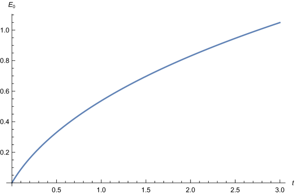
Figure 3: Plot of the threshold energy $E_{0}$ as a function of $t=g_{\rm s}K$. We set $z=1$ in this figure.

Once we know $E_{0}$, we can numerically evaluate the integral (83) to find $\rho_{0}(E)$. In Figure 4, we show the plot of $\rho_{0}(E)$ for $t=3,z=1,g_{\rm s}=1$ as an example. As a comparison, we also plot the pure JT gravity density of states (85) (see orange dashed curve in Figure 4).

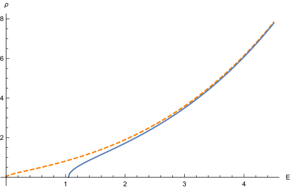
Figure 4: Plot of the eigenvalue density $\rho_{0}(E)$ for $t=3,z=1,g_{s}=1$ (blue solid curve). The orange dashed curve represents the pure JT gravity density of states in (85).

When $z^{2}>0$, the eigenvalue corresponding to the FZZT brane is located at $E=-z^{2}/2<0$. Since the eigenvalues behave as fermions and they repel each other, the other eigenvalues are pushed toward the positive $E$ direction, as we can see from Figure 4.

On the other hand, if $E=-z^{2}/2>0$ the corresponding eigenvalue is inserted on the original support of the pure JT gravity eigenvalue density (85). We expect this insertion creates a void in the support of $\rho_{0}(E)$. As we increase $t$, we expect that the support of eigenvalue density is split into two parts and the model exhibits a phase transition from a one-cut phase to a two-cut phase. However, in our formalism (20) of the perturbative treatment of FZZT branes we assumed $\text{Re}(z^{2})>0$ for the derivation of $\mathcal{M}(b)=-e^{-zb}$ in (17). In other words, our formalism (20) is valid only for the one-cut phase of the matrix model. To see the effect of FZZT branes with $\text{Re}(z^{2})<0$ we need a non-perturbative treatment of FZZT branes, which we will consider in section 5.

Before closing this subsection, let us compute the order $\mathcal{O}(t^{1})$ correction of the density of states (83). One can show that

$$\rho_{0}(E)\Big{|}_{\mathcal{O}(t)} =\frac{1}{\sqrt{2}\pi g_{\rm s}}\left(-\frac{t}{z\sqrt{E}}+\frac{2t\sqrt{E}}{(z^{2}+2E)z}\right)$$ (90)

$$=-\frac{t}{\sqrt{2}\pi g_{\rm s}}\frac{z}{(z^{2}+2E)\sqrt{E}}.$$

Then the order $\mathcal{O}(t)$ correction to the one-point function $\langle Z(\beta)\rangle$ is given by

$$\int_{0}^{\infty}dEe^{-\beta E}\rho_{0}(E)\Big{|}_{\mathcal{O}(t)} =-\frac{t}{2g_{\rm s}}e^{\frac{1}{2}z^{2}\beta}\text{Erfc}\left(\sqrt{\frac{z^{2}\beta}{2}}\right)=KZ_{\text{HW}}(\beta,z),$$ (91)

where $Z_{\text{HW}}(\beta,z)$ is the “half-wormhole” amplitude in (57). In (91) $Z_{\text{HW}}(\beta,z)$ is multiplied by a factor of $K$ since we are considering $K$ FZZT branes. Thus our expression of the genus-zero density of states in (83) correctly reproduces the half-wormhole contribution in (57).

3.2 String equation via the Lagrange reversion

As discussed in Maxfield:2020ale , the modification of the genus-zero string equation $f(u)=0$ with $f(u)$ in (82) can also be seen by using the Lagrange reversion theorem. Following Maxfield:2020ale , let us consider the modification of the genus-zero part of the two-point function $\langle Z(\beta_{1})Z(\beta_{2})\rangle_{\rm c}^{g=0}$ due to the insertion of $K$ FZZT branes $\det(z^{2}/2+H)^{K}$. By using our formalism (20) in the general background $\{t_{k}\}$, the genus-zero two-point function in the presence of $K$ FZZT branes is written as

$$\langle Z(\beta_{1})Z(\beta_{2})\det(z^{2}/2+H)^{K}\rangle_{\rm c}^{g=0}$$ (92)

$$= \frac{\sqrt{\beta_{1}\beta_{2}}}{2\pi(\beta_{1}+\beta_{2})}e^{(\beta_{1}+\beta_{2})u_{0}}$$

$$+\sum_{n=1}^{\infty}\frac{g_{\rm s}^{n}}{n!}\prod_{i=1}^{2}\int_{0}^{\infty}b_{i}^{\prime}db_{i}^{\prime}Z_{\text{trumpet}}(\beta_{i},b_{i}^{\prime})\prod_{j=1}^{n}\int_{0}^{\infty}db_{j}\mathcal{M}(b_{j})V_{0,n+2}(b_{1}^{\prime},b_{2}^{\prime},b_{1},\cdots,b_{n}),$$

where $V_{0,n+2}(\bm{b})$ is given by (48) and $\mathcal{M}(b)$ for $K$ FZZT branes is given by

$$\mathcal{M}(b)=-Ke^{-zb}.$$ (93)

By using (45) and (47), (92) is written as

$$\langle Z(\beta_{1})Z(\beta_{2})\det(z^{2}/2+H)^{K}\rangle_{\rm c}^{g=0}$$ (94)

$$= \frac{\sqrt{\beta_{1}\beta_{2}}}{2\pi(\beta_{1}+\beta_{2})}e^{(\beta_{1}+\beta_{2})u_{0}(t_{0})}$$

$$+\frac{\sqrt{\beta_{1}\beta_{2}}}{2\pi}\sum_{n=1}^{\infty}\frac{(-t)^{n}}{n!}\partial_{0}^{n-1}\Bigl{(}\partial_{0}u_{0}(t_{0})e^{(\beta_{1}+\beta_{2})u_{0}(t_{0})}(z^{2}-2u_{0}(t_{0}))^{-\frac{n}{2}}\Bigr{)}$$

$$= \frac{\sqrt{\beta_{1}\beta_{2}}}{2\pi(\beta_{1}+\beta_{2})}\left[e^{(\beta_{1}+\beta_{2})u_{0}(t_{0})}+\sum_{n=1}^{\infty}\frac{(-t)^{n}}{n!}\partial_{0}^{n-1}\Bigl{(}\partial_{0}e^{(\beta_{1}+\beta_{2})u_{0}(t_{0})}(z^{2}-2u_{0}(t_{0}))^{-\frac{n}{2}}\Bigr{)}\right],$$

where $t_{0}$-dependence has been explicitly expressed for convenience of explanation. Let us now recall the Lagrange reversion theorem (see e.g. Whittaker ): Suppose that $\zeta$ is related to $a$ by the equation

$$\zeta=a+t\phi(\zeta)$$ (95)

with $\phi(z)$ being some function. Then for any function $g(z)$ and for small enough $t$, $g(\zeta)$ is expanded as

$$g(\zeta)=g(a)+\sum_{n=1}^{\infty}\frac{t^{n}}{n!}\frac{d^{n-1}}{da^{n-1}}\left[g^{\prime}(a)\{\phi(a)\}^{n}\right].$$ (96)

Using this theorem one immediately sees that (94) is rewritten as

$$\langle Z(\beta_{1})Z(\beta_{2})\det(z^{2}/2+H)^{K}\rangle_{\rm c}^{g=0}=\frac{\sqrt{\beta_{1}\beta_{2}}}{2\pi(\beta_{1}+\beta_{2})}e^{(\beta_{1}+\beta_{2})u_{0}(x)}$$ (97)

with

$$x=t_{0}-\frac{t}{\sqrt{z^{2}-u_{0}(x)}}.$$ (98)

Now, the genus zero string equation $u_{0}-I_{0}(u_{0})=0$ is written in the off-shell JT gravity background $t_{k}=\gamma_{k}\ (k\geq 1)$ as

$$0=\sqrt{u_{0}(t_{0})}J_{1}\left(2\sqrt{u_{0}(t_{0})}\right)-t_{0}.$$ (99)

Writing this equation at $t_{0}=x$ with $x$ in (98) and then setting $t_{0}=0$ to restrict ourselves to the on-shell JT gravity background, we have

$$\begin{aligned} 0&=\sqrt{u_{0}(x)}J_{1}\left(2\sqrt{u_{0}(x)}\right)-x\\ &=\sqrt{u_{0}(x)}J_{1}\left(2\sqrt{u_{0}(x)}\right)+\frac{t}{\sqrt{z^{2}-u_{0}(x)}}.\end{aligned}$$ (100)

We have thus seen that the genus zero two-point function in the presence of $K$ FZZT-branes is written as the genuine genus zero two-point function (97) with $u_{0}(x)$ satisfying the equation (100). This is identical with the modified string equation $f(u_{0}(x))=0$ with $f(u)$ given in (82), which was obtained from the shift of couplings (81).

3.3 Comment on dilaton gravity

In Witten:2020wvy ; Maxfield:2020ale , it is shown that we can add conical defects in JT gravity by modifying the dilaton potential

$$S=-\frac{1}{2}\int d^{2}x\sqrt{g}\Bigl{[}\phi(R+2)+U(\phi)\Bigr{]}.$$ (101)

For the defects with deficit angle $2\pi\alpha_{i}$ with fugacity $\varepsilon_{i}$, $U(\phi)$ is given by

$$U(\phi)=2\sum_{i}\varepsilon_{i}e^{-2\pi(1-\alpha_{i})\phi}.$$ (102)

As discussed in Maxfield:2020ale the effect of defects is summarized as the modification of the string equation (see also Budd ; Johnson:2020lns ; Forste:2021roo )

$$u-I_{0}(u)=\sqrt{u}J_{1}(2\sqrt{u})-\sum_{i}\varepsilon_{i}J_{0}(2\alpha_{i}\sqrt{u}).$$ (105)

From this we can read off the shifted coupling as

$$t_{k}=\gamma_{k}+\sum_{i}\varepsilon_{i}\frac{(-1)^{k}\alpha_{i}^{2k}}{k!}.$$ (106)

Let us consider the relation between this shifted coupling and the dilaton potential $U(\phi)$. To see this, it is convenient to define

$$\widetilde{U}(\phi) =U(\phi)e^{2\pi\phi},\quad\widetilde{U}_{+}(\phi) =\frac{\widetilde{U}(\phi)+\widetilde{U}(-\phi)}{2}.$$ (107)

For the dilaton potential in (102) we find

$$\widetilde{U}_{+}(\phi)=2\sum_{i}\varepsilon_{i}\cosh(2\pi\alpha_{i}\phi).$$ (108)

From (106), this is also written as

$$\widetilde{U}_{+}(\phi) =2\sum_{k=0}^{\infty}\frac{(-1)^{k}(t_{k}-\gamma_{k})}{(2k-1)!!}\frac{(2\pi\phi)^{2k}}{2^{k}}.$$ (109)

As argued in Witten:2020wvy , the equivalence of the matrix model and dilaton gravity holds for a wide class of dilaton potential written as a superposition of the defect potential (102)

$$U(\phi)=2\int d\alpha\varepsilon(\alpha)e^{-2\pi(1-\alpha)\phi}.$$ (110)

Thus we expect that (109) can be applied to a wide class of background couplings $\{t_{k}\}$. For instance, if we add $K$ FZZT branes the coupling is shifted as (81). Plugging (81) into (109), the corresponding dilaton potential becomes

$$\widetilde{U}_{+}(\phi)=-\frac{2tz}{z^{2}+2\pi^{2}\phi^{2}}.$$ (111)

In this approach we can only find the even part of $\widetilde{U}(\phi)=U(\phi)e^{2\pi\phi}$. We do not know how to recover the odd part of $\widetilde{U}(\phi)$ from the data of $\{t_{k}\}$.

Also, it is not clear to us what is the condition for the applicability of the formula (109). We do not know how far we can deform the coupling from the JT gravity background $t_{k}=\gamma_{k}$ when we use (109). Putting this problem aside, if we naively apply (109) to the $(2,p)$ minimal model background (234) we find

$$\widetilde{U}_{+}(\phi)=2\pi\phi\sinh\left[p\,\text{arcsinh}\left(\frac{2\pi\phi}{p}\right)\right]-2\pi\phi\sinh(2\pi\phi).$$ (112)

In the $p\to\infty$ limit, $\widetilde{U}_{+}(\phi)$ in (112) vanishes, which is consistent with the statement that JT gravity is a $p\to\infty$ limit of the $(2,p)$ minimal string Seiberg:2019 ; Saad:2019lba .

In Seiberg:2019 ; Mertens:2020hbs ; Turiaci:2020fjj , it is proposed that a dilaton gravity theory with $\sinh\phi$ potential corresponds to the $(2,p)$ minimal string. It would be interesting to understand the relation between our (112) and the proposal in Seiberg:2019 ; Mertens:2020hbs ; Turiaci:2020fjj , if any.

4 Baker-Akhiezer function and FZZT branes

In this section we review the known results about the Baker-Akhiezer (BA) function, the Christoffel-Darboux (CD) kernel and the multi-FZZT amplitude.

4.1 Multi-FZZT amplitude from matrix integral

As discussed in Maldacena:2004sn , the BA function can be thought of as the wavefunction of FZZT brane, which is obtained as a double-scaling limit of the orthogonal polynomial. In the matrix model at finite $N$

$$Z_{N}=\int_{N\times N}dMe^{-\operatorname{Tr}V(M)},$$ (113)

it is convenient to define the polynomial $P_{n}(\lambda)=\lambda^{n}+\cdots$ of degree $n$ which is orthogonal with respect to the weight $e^{-V(\lambda)}$

$$\int d\lambda e^{-V(\lambda)}P_{n}(\lambda)P_{m}(\lambda)=h_{n}\delta_{n,m}.$$ (114)

One can show that $Z_{N}$ in (113) is written in terms of the norm $h_{n}$ of the orthogonal polynomial $P_{n}(\lambda)$

$$Z_{N}=\prod_{n=0}^{N-1}h_{n}.$$ (115)

It is convenient to define the normalized orthogonal polynomial by

$$\psi_{n}(\lambda)=\frac{e^{-\frac{1}{2}V(\lambda)}}{\sqrt{h_{n}}}P_{n}(\lambda),$$ (116)

which satisfies

$$\int d\lambda\psi_{n}(\lambda)\psi_{m}(\lambda)=\delta_{n,m}.$$ (117)

It is well known that $\psi_{N}(\lambda)$ is given by the expectation value of the determinant operator in the matrix model (see e.g. Eynard:2015aea for a review)

$$\psi_{N}(\lambda) =\langle\Psi_{N}(\lambda)\rangle=\frac{1}{Z_{N}}\int_{N\times N}dMe^{-\operatorname{Tr}V(M)}\Psi_{N}(\lambda),$$ (118)

where $\Psi_{N}(\lambda)$ is given by

$$\Psi_{N}(\lambda)=\frac{e^{-\frac{1}{2}V(\lambda)}}{\sqrt{h_{N}}}\det_{N\times N}(\lambda-M).$$ (119)

Another important ingredient is the CD kernel

$$K_{N}(\xi,\eta) =\sum_{n=0}^{N-1}\psi_{n}(\xi)\psi_{n}(\eta).$$ (120)

Using the relation

$$\lambda\psi_{n}(\lambda)=\sqrt{r_{n+1}}\psi_{n+1}(\lambda)+\sqrt{r_{n}}\psi_{n-1}(\lambda),\quad r_{n}=\frac{h_{n}}{h_{n-1}},$$ (121)

the CD kernel is written as

$$K_{N}(\xi,\eta)=\sqrt{r_{N}}\frac{\psi_{N}(\xi)\psi_{N-1}(\eta)-\psi_{N-1}(\xi)\psi_{N}(\eta)}{\xi-\eta}.$$ (122)

One can show that the CD kernel (120) is given by the two-point function of determinant operators

$$K_{N}(\xi,\eta)=\langle\Psi_{N-1}(\xi)\Psi_{N-1}(\eta)\rangle,$$ (123)

where the expectation value is taken in the $(N-1)\times(N-1)$ matrix integral. In the double-scaling limit the index $n$ of $\psi_{n}(\lambda)$ becomes a continuous coordinate $t_{0}$

$$\psi_{n}(\lambda)\quad\to\quad\psi(\lambda;t_{0}),$$ (124)

and the double-scaling limit of (120) becomes

$$K(\xi,\eta)=\frac{1}{\hbar}\int_{-\infty}^{t_{0}}dx\psi(\xi;x)\psi(\eta;x).$$ (125)

Here $\hbar$ is related to the genus counting parameter $g_{\rm s}$ by

$$\hbar=\frac{g_{\rm s}}{\sqrt{2}}.$$ (126)

From (125), one can see that $K(\xi,\eta)$ satisfies

$$\hbar\partial_{0}K(\xi,\eta)=\psi(\xi)\psi(\eta),$$ (127)

where $\psi(\xi)=\psi(\xi;t_{0})$. One can also show that (121) reduces to the Schrödinger equation in the double-scaling limit (see Ginsparg:1993is for a review)

$$\big{(}\hbar^{2}\partial_{0}^{2}+u\big{)}\psi(\lambda)=\lambda\psi(\lambda),$$ (128)

where $u$ is the specific heat

$$u=g_{\rm s}^{2}\partial_{0}^{2}F=2\hbar^{2}\partial_{0}^{2}F.$$ (129)

Note that the CD kernel of the form (122) in the double scaling limit becomes

$$K(\xi,\eta)=\hbar\frac{\partial_{0}\psi(\xi)\psi(\eta)-\psi(\xi)\partial_{0}\psi(\eta)}{\xi-\eta}.$$ (130)

This is also derived from (125) by using (128).

As discussed in Maldacena:2004sn the multi-point function of FZZT branes can be obtained by taking the double scaling limit of the finite $N$ expression Morozov:1994hh ; Brezin:2000

$$\left\langle\prod_{i=1}^{k}\det(\xi-M)\right\rangle_{N\times N}=\frac{1}{\Delta(\xi)}\det\Bigl{(}P_{N+i-1}(\xi_{j})\Bigr{)}_{i,j=1,\ldots,k},$$ (131)

where $\Delta(\xi)=\prod_{i<j}(\xi_{i}-\xi_{j})$ is the Vandermonde determinant. In the double scaling limit one finds Maldacena:2004sn

$$\left\langle\prod_{i=1}^{k}\Psi(\xi)\right\rangle=\frac{\Delta(d)}{\Delta(\xi)}\prod_{i=1}^{k}\psi(\xi_{i}).$$ (132)

Here $d_{j}$ is the shorthand for the action of $d=\hbar\partial_{0}$ on $\psi(\xi_{j})$.

4.2 Genus expansion of BA function

Let us consider the genus expansion of the BA function $\psi(\xi)=\psi(\xi;t_{0})$. It is known that the BA function is written as a ratio of tau-function $\tau(\bm{t})=e^{F(\bm{t})}$ Date:1982yeu ; dubrovin :

$$\psi(\xi)=e^{\vartheta(z)}\frac{\tau(\bm{t}-[z^{-1}])}{\tau(\bm{t})}=e^{\vartheta(z)+F(\bm{t}-[z^{-1}])-F(\bm{t})},$$ (133)

where $\xi=z^{2}/2$ and

$$\vartheta(z)=\frac{1}{g_{\rm s}}\sum_{k=0}^{\infty}\frac{t_{k}-\delta_{k,1}}{(2k+1)!!}z^{2k+1}.$$ (134)

$[z^{-1}]$ in (133) is defined by

$${}[z^{-1}]_{k}=g_{\rm s}(2k-1)!!z^{-2k-1}.$$ (135)

This is consistent with our result of the shift of couplings (42).

Let us consider the genus expansion of the BA function

$$\log\psi(\xi)=\vartheta(z)+F(\bm{t}-[z^{-1}])-F(\bm{t})=\sum_{n=0}^{\infty}g_{\rm s}^{n-1}A_{n}.$$ (136)

The $A_{0}$ term is known as the effective potential

$$A_{0}=-\frac{1}{2}V_{\text{eff}}(\xi),$$ (137)

whose explicit form is obtained in Okuyama:2020ncd as

$$\frac{1}{2}V_{\text{eff}}(\xi)=\sum_{n=1}^{\infty}\frac{\delta_{n,1}-I_{n}}{(2n+1)!!}(z^{2}-2u_{0})^{n+\frac{1}{2}}.$$ (138)

On the other hand, from (136) we find

$$\frac{1}{2}V_{\text{eff}}(\xi)=\sum_{k=0}^{\infty}\left[\frac{\delta_{k,1}-t_{k}}{(2k+1)!!}z^{2k+1}+\frac{(2k-1)!!}{z^{2k+1}}\partial_{k}F_{0}\right].$$ (139)

We can show the equivalence of (138) and (139) as follows. It turns out that (138) has the following integral representation

$$\frac{1}{2}V_{\text{eff}}(\xi)=\int_{u_{0}}^{z^{2}/2}du\frac{u-I_{0}(u)}{\sqrt{z^{2}-2u}}.$$ (140)

This can be shown by using the relations

$$\partial_{u}I_{k}(u)=I_{k+1}(u),\quad u_{0}-I_{0}(u_{0})=0$$ (141)

and repeating the partial integration:

$$\frac{1}{2}V_{\text{eff}}(\xi) =-(u-I_{0}(u))(z^{2}-2u)^{\frac{1}{2}}\Big{|}_{u=u_{0}}^{u=\frac{z^{2}}{2}}+\int_{u_{0}}^{z^{2}/2}du(1-I_{1}(u))(z^{2}-2u)^{\frac{1}{2}}$$ (142)

$$=-\frac{1-I_{1}(u)}{3}(z^{2}-2u)^{\frac{3}{2}}\Big{|}_{u=u_{0}}^{u=\frac{z^{2}}{2}}-\int_{u_{0}}^{z^{2}/2}du\frac{I_{2}(u)}{3}(z^{2}-2u)^{\frac{3}{2}}$$

$$=\frac{1-I_{1}(u_{0})}{3}(z^{2}-2u_{0})^{\frac{3}{2}}+\frac{I_{2}(u)}{5!!}(z^{2}-2u)^{\frac{5}{2}}\Big{|}_{u=u_{0}}^{u=\frac{z^{2}}{2}}-\int_{u_{0}}^{z^{2}/2}du\frac{I_{3}(u)}{5!!}(z^{2}-2u)^{\frac{5}{2}}$$

$$=\cdots=\sum_{n=1}^{\infty}\frac{\delta_{n,1}-I_{n}}{(2n+1)!!}(z^{2}-2u_{0})^{n+\frac{1}{2}}.$$

Now, let us decompose (140) into two parts

$$\frac{1}{2}V_{\text{eff}}(\xi) =\int_{0}^{z^{2}/2}du\frac{u-I_{0}(u)}{\sqrt{z^{2}-2u}}-\int_{0}^{u_{0}}du\frac{u-I_{0}(u)}{\sqrt{z^{2}-2u}}$$ (143)

One can show that the first term of (143) agrees with the first term of (139)

$$\int_{0}^{z^{2}/2}du\frac{u-I_{0}(u)}{\sqrt{z^{2}-2u}} =\int_{0}^{z^{2}/2}du\sum_{k=0}^{\infty}(\delta_{k,1}-t_{k})\frac{u^{k}}{k!}(z^{2}-2u)^{-\frac{1}{2}}$$ (144)

$$=\sum_{k=0}^{\infty}\frac{\delta_{1,k}-t_{k}}{(2k+1)!!}z^{2k+1}.$$

Using the relation Itzykson:1992ya

$$F_{0}=\frac{1}{2}\int_{0}^{u_{0}}du(I_{0}(u)-u)^{2},$$ (145)

one can show that the second term of (143) is equal to the second term of (139). Thus we find the equivalence of (138) and (139).

We can compute the higher genus corrections of the genus expansion (136) by introducing the operator

$$D(z)=-\sum_{k=0}^{\infty}(2k-1)!!z^{-2k-1}\partial_{k}.$$ (146)

Then we find

$$\log\psi=\vartheta(z)+\sum_{g=0}^{\infty}\sum_{n=1}^{\infty}g_{s}^{2g-2+n}\frac{D(z)^{n}}{n!}F_{g}.$$ (147)

For instance, the first few terms are given by

$$A_{0} =g_{\rm s}\vartheta(z)+D(z)F_{0},$$ (148)

$$A_{1} =\frac{1}{2}D(z)^{2}F_{0},$$

$$A_{2} =\frac{1}{6}D(z)^{3}F_{0}+D(z)F_{1}.$$

In this computation, the following relations are useful

$$D(z)I_{k}(u) =-\frac{(2k-1)!!}{(z^{2}-2u)^{k+\frac{1}{2}}},\quad D(z)u_{0}=-\frac{1}{t\widetilde{z}},$$ (149)

where

$$\widetilde{z}=\sqrt{z^{2}-2u_{0}}.$$ (150)

From (149) and $F_{1}=-\frac{1}{24}\log t$ one can show that

$$A_{1} =-\frac{1}{2}\log\widetilde{z}+\frac{1}{2}\log z,$$ (151)

$$A_{2} =-\frac{5}{24t\widetilde{z}^{3}}-\frac{I_{2}}{24t^{2}\widetilde{z}}.$$

This reproduces the known result of the genus expansion of BA function Okuyama:2020ncd (up to the normalization), as expected.

4.3 Genus expansion of the multi-FZZT amplitude

The multi-FZZT amplitude is written as

$$\left\langle\prod_{i}\Psi(\xi_{i})\right\rangle=\frac{\Delta(z)}{\Delta(\xi)}e^{\sum_{i}\vartheta(z_{i})+F(\bm{t}-\sum_{i}[z_{i}^{-1}])-F(\bm{t})}\equiv\frac{\Delta(z)}{\Delta(\xi)}e^{A(z_{i})}$$ (152)

The genus expansion of $A(z_{i})$ can be obtained as follows. The Itzykson-Zuber variable for $\widetilde{t}_{k}$ in (42) is written as

$$\widetilde{I}_{k}(\widetilde{u}_{0})=\sum_{n=0}^{\infty}\widetilde{t}_{k+n}\frac{\widetilde{u}_{0}^{n}}{n!}=I_{k}(\widetilde{u}_{0})-g_{\rm s}(2k-1)!!\sum_{i}(z^{2}_{i}-2\widetilde{u}_{0})^{-k-\frac{1}{2}}.$$ (153)

The string equation for the shifted background $\widetilde{t}_{k}$ becomes

$$\widetilde{u}_{0}-I_{0}(\widetilde{u}_{0})+\sum_{i}\frac{g_{\rm s}}{\sqrt{z^{2}_{i}-2\widetilde{u}_{0}}}=0.$$ (154)

From (154) we find the genus expansion of $\widetilde{u}_{0}$

$$\widetilde{u}_{0}=u_{0}-\sum_{i}\frac{g_{\rm s}}{t\widetilde{z}_{i}}+\cdots,\qquad\widetilde{z}_{i}=\sqrt{z^{2}_{i}-2u_{0}}.$$ (155)

Then the genus expansion of $F(\bm{t}-\sum_{i}[z_{i}^{-1}])$ is obtained by replacing $I_{k}(u_{0})$ in $F(\bm{t})$ by $\widetilde{I}_{k}(\widetilde{u}_{0})$. Thus we have

$$A(z_{i})=\sum_{i}\vartheta(z_{i})+F(\widetilde{I}_{k}(\widetilde{u}_{0}))-F(I_{k}(u_{0})).$$ (156)

Recall that $F_{g}(t)~{}(g\geq 2)$ are given by polynomials of $I_{k}(u_{0})~{}(k\geq 2)$ and $(1-I_{1}(u_{0}))^{-1}$ Itzykson:1992ya . For $g=0$ and $g=1$ we have

$$F_{0}(\bm{t}-\sum_{i}[z_{i}^{-1}]) =\frac{1}{2}\int_{0}^{\widetilde{u}_{0}}du\left[I_{0}(u)-\sum_{i}\frac{g_{\rm s}}{\sqrt{z^{2}_{i}-2u}}-u\right]^{2},$$ (157)

$$F_{1}(\bm{t}-\sum_{i}[z^{-1}]) =-\frac{1}{24}\log\left(1-I_{0}(\widetilde{u}_{0})+\sum_{i}\frac{g_{\rm s}}{(z^{2}_{i}-2\widetilde{u}_{0})^{3/2}}\right).$$

Expanding these expressions using (155), we can compute the genus expansion of $A(z_{i})$ in (152).

4.4 Annulus amplitude between two FZZT branes

Let us consider the annulus amplitude between two FZZT branes. From (152) we have

$$\langle\Psi(\xi_{1})\Psi(\xi_{2})\rangle=\frac{z_{1}-z_{2}}{\xi_{1}-\xi_{2}}e^{A(z_{1},z_{2})}=\frac{2}{z_{1}+z_{2}}e^{A(z_{1},z_{2})}.$$ (158)

The prefactor agrees with the exponentiated annulus amplitude (78) up to an overall normalization constant. On the other hand, from (132) we find

$$\langle\Psi(\xi_{1})\Psi(\xi_{2})\rangle=\frac{\hbar\partial_{0}A(z_{1})-\hbar\partial_{0}A(z_{2})}{\xi_{1}-\xi_{2}}e^{A(z_{1})+A(z_{2})}.$$ (159)

At the leading order in the genus expansion, the prefactor becomes

$$\frac{\hbar}{g_{\rm s}}\frac{\partial_{0}A_{0}(z_{1})-\partial_{0}A_{0}(z_{2})}{\xi_{1}-\xi_{2}} =\sqrt{2}\frac{\widetilde{z}_{1}-\widetilde{z}_{2}}{z_{1}^{2}-z_{2}^{2}}=\frac{\sqrt{2}}{\widetilde{z}_{1}+\widetilde{z}_{2}},$$ (160)

where we used the relation obtained from (138)

$$\partial_{0}A_{0}(z)=\widetilde{z}.$$ (161)

The difference between the prefactors of (158) and (160) is compensated by

$$\Bigl{[}A(z_{1},z_{2})-A(z_{1})-A(z_{2})\Bigr{]}_{\mathcal{O}(g_{\rm s}^{0})}$$ (162)

$$= \frac{1}{2}\left[D(z_{1})+D(z_{2})\right]^{2}F_{0}-\frac{1}{2}D(z_{1})^{2}F_{0}-\frac{1}{2}D(z_{2})^{2}F_{0}$$

$$= D(z_{1})D(z_{2})F_{0}$$

$$= \int_{0}^{u_{0}}\frac{du}{\sqrt{(z^{2}_{1}-2u)(z_{2}^{2}-2u)}}$$

$$= \log\left(\frac{z_{1}+z_{2}}{\widetilde{z}_{1}+\widetilde{z}_{2}}\right).$$

Thus the two expressions (158) and (160) are consistent at this order.

4.5 FZZT amplitude and CD kernel

As shown in Strahov:2002zu , the correlator of $2k$ determinants in the finite $N$ matrix model is written in terms of the CD kernel as

$$\Bigl{\langle}\prod_{i=1}^{k}\Psi_{N}(\xi_{i})\Psi_{N}(\eta_{i})\Bigr{\rangle} =\frac{\det\bigl{(}K_{N+k}(\xi_{i},\eta_{j})\bigr{)}}{\Delta(\xi)\Delta(\eta)}$$ (163)

$$=\frac{1}{\Delta(\xi)\Delta(\eta)}\left|\begin{matrix}K_{N+k}(\xi_{1},\eta_{1})&\cdots&K_{N+k}(\xi_{1},\eta_{k})\\ K_{N+k}(\xi_{2},\eta_{1})&\cdots&K_{N+k}(\xi_{2},\eta_{k})\\ \vdots&\cdots&\vdots\\ K_{N+k}(\xi_{k},\eta_{1})&\cdots&K_{N+k}(\xi_{k},\eta_{k})\end{matrix}\right|.$$

For the odd number of determinants, the correlator can be obtained by sending $\eta_{k}\to\infty$ in (163)

$$\Bigl{\langle}\prod_{i=1}^{k}\Psi_{N}(\xi_{i})\prod_{j=1}^{k-1}\Psi_{N}(\eta_{j})\Bigr{\rangle} =\frac{\det\bigl{(}K_{N+k}(\xi_{i},\eta_{j})\big{|}\psi_{N+k-1}(\xi_{i})\bigr{)}}{\Delta(\xi)\Delta(\eta)}$$ (164)

$$=\frac{1}{\Delta(\xi)\Delta(\eta)}\left|\begin{matrix}K_{N+k}(\xi_{1},\eta_{1})&\cdots&K_{N+k}(\xi_{1},\eta_{k-1})&\psi_{N+k-1}(\xi_{1})\\ K_{N+k}(\xi_{2},\eta_{1})&\cdots&K_{N+k}(\xi_{2},\eta_{k-1})&\psi_{N+k-1}(\xi_{2})\\ \vdots&\cdots&\vdots&\vdots\\ K_{N+k}(\xi_{k},\eta_{1})&\cdots&K_{N+k}(\xi_{k},\eta_{k-1})&\psi_{N+k-1}(\xi_{k})\end{matrix}\right|.$$

In the double scaling limit, we find

$$\Bigl{\langle}\prod_{i=1}^{k}\Psi(\xi_{i})\Psi(\eta_{i})\Bigr{\rangle} =\frac{\det\bigl{(}K(\xi_{i},\eta_{j})\bigr{)}}{\Delta(\xi)\Delta(\eta)},$$ (165)

$$\Bigl{\langle}\prod_{i=1}^{k}\Psi(\xi_{i})\prod_{j=1}^{k-1}\Psi(\eta_{j})\Bigr{\rangle} =\frac{\det\bigl{(}K(\xi_{i},\eta_{j})\big{|}\psi(\xi_{i})\bigr{)}}{\Delta(\xi)\Delta(\eta)},$$

where $\psi(\xi)$ and $K(\xi,\eta)$ are the BA function and the CD kernel (125), respectively. In other words, the correlator of the even number of FZZT branes can be written as a product of two-point functions $K(\xi,\eta)$. Although the permutation symmetry of the parameters $\xi_{i}$ and $\eta_{i}$ is not manifest in (165), the result is symmetric as proved in Strahov:2002zu . Of course, one can use (132) for the multi-point function of FZZT branes. However, $\partial_{0}^{n}\psi(\xi)$ with $n\geq 2$ can be reduced to a linear combination of $\psi(\xi)$ and $\partial_{0}\psi(\xi)$ using the Schrödinger equation (128), and after this rewriting one finds that (132) is identical with (165).

5 Correlator of FZZT branes and macroscopic loops

In this section, we consider the correlator of FZZT branes $\Psi(\xi_{i})$ and macroscopic loop operators $Z(\beta_{j})$.

5.1 Bra–ket notation

To describe our results, it is convenient to introduce the bra–ket notation as follows.

Let $\hat{x}$ be the coordinate operator and $\hat{\partial}_{x}$ be its conjugate “momentum operator” satisfying

$${}[\hat{\partial}_{x},\hat{x}]=1.$$ (166)

We then introduce the operator

$$Q:=\hbar^{2}\hat{\partial}_{x}^{2}+\hat{u},\qquad\hat{u}:=u\Big{|}_{t_{0}=\hat{x}},$$ (167)

where $u$ is the specific heat (129). We decided not to put a hat $\hat{}\,$ on $Q$ just for notational simplicity.

For a Roman letter $x$, we let $|x\rangle$ denote the coordinate eigenstate, e.g.

$$\hat{x}|x\rangle=x|x\rangle,\qquad\hat{x}|t_{0}\rangle=t_{0}|t_{0}\rangle.$$ (168)

For a Greek letter $\xi$, on the other hand, we let $|\xi\rangle$ denote an eigenstate of $Q$ with eigenvalue $\xi$:

$$Q|\xi\rangle=\xi|\xi\rangle.$$ (169)

These states are normalized such that

$$1=\int_{-\infty}^{\infty}d\xi|\xi\rangle\langle\xi|,\qquad\psi(\xi;x)=\langle x|\xi\rangle=\langle\xi|x\rangle,$$ (170)

where $\psi(\xi;x)$ is the BA function. Another important element is the projection operator

$$\Pi:=\frac{1}{\hbar}\int_{-\infty}^{t_{0}}dx|x\rangle\langle x|.$$ (171)

As discussed in Banks:1989df , $\Pi$ can be interpreted as the projection below the Fermi level $t_{0}$. In terms of $\Pi$ the CD kernel (125) is expressed as

$$K(\xi,\eta)=\langle\xi|\Pi|\eta\rangle.$$ (172)

Note that $\Pi$ satisfies

$$\hbar\partial_{0}\Pi=|t_{0}\rangle\langle t_{0}|.$$ (173)

Note also that $\langle t_{0}|$ and $|t_{0}\rangle$ satisfy

$$\langle t_{0}|Q=(\hbar^{2}\partial_{0}^{2}+u)\langle t_{0}|,\qquad Q|t_{0}\rangle=(\hbar^{2}\partial_{0}^{2}+u)|t_{0}\rangle,$$ (174)

so that the Schrödinger equation (128) holds.

5.2 Correlator of one FZZT brane and macroscopic loops

As a first step, we consider the correlator of one FZZT brane and macroscopic loops. Following Blommaert:2019wfy , let us consider the correlator of $\det(\xi-M)$ and $\operatorname{Tr}e^{\beta M}$ at finite $N$:

$$\big{\langle}\operatorname{Tr}e^{\beta M}\Psi_{N}(\xi)\big{\rangle}$$ (175)

$$= \frac{1}{N!Z_{N}}\int\prod_{i=1}^{N}d\lambda_{i}e^{-V(\lambda_{i})}\Delta(\lambda)^{2}\sum_{i=1}^{N}e^{\beta\lambda_{i}}\frac{e^{-\frac{1}{2}V(\xi)}}{\sqrt{h_{N-1}}}\prod_{i=1}^{N}(\xi-\lambda_{i})$$

$$= \frac{1}{(N-1)!Z_{N-1}}$$

$$\times\int d\lambda e^{\beta\lambda}(\xi-\lambda)\int\prod_{i=1}^{N-1}d\lambda_{i}^{\prime}e^{-V(\lambda_{i}^{\prime})}\Delta(\lambda^{\prime})^{2}\frac{e^{-V(\lambda)}}{h_{N-1}}\frac{e^{-\frac{1}{2}V(\xi)}}{\sqrt{h_{N-1}}}\prod_{i=1}^{N-1}(\lambda-\lambda_{i}^{\prime})^{2}(\xi-\lambda_{i}^{\prime})$$

$$= (r_{N-1}^{3})^{-\frac{1}{2}}\int d\lambda e^{\beta\lambda}(\xi-\lambda)\big{\langle}\Psi_{N-1}(\lambda)^{2}\Psi_{N-1}(\xi)\big{\rangle},$$

where $Z_{N}$ is given by (115) and $M$ is related to $H$ by $M=-H$ (see footnote 2). It follows from (165) that in the double scaling limit this becomes

$$\langle Z(\beta)\Psi(\xi)\rangle =\int d\lambda e^{\beta\lambda}(\xi-\lambda)\frac{1}{\xi-\lambda}\left|\begin{matrix}K(\lambda,\lambda)&\psi(\lambda)\\ K(\xi,\lambda)&\psi(\xi)\end{matrix}\right|$$ (176)

$$=\int d\lambda e^{\beta\lambda}\Bigl{[}K(\lambda,\lambda)\psi(\xi)-K(\xi,\lambda)\psi(\lambda)\Bigr{]}.$$

In appendix B, we will give an alternative derivation of this result. Note that $\rho(\lambda)=K(\lambda,\lambda)$ is the eigenvalue density. Thus the first term of (176) is the disconnected part $\langle Z(\beta)\rangle\langle\Psi(\xi)\rangle$ and the second term is the connected part

$$\langle Z(\beta)\Psi(\xi)\rangle_{\rm c} =-\int d\lambda e^{\beta\lambda}\psi(\lambda)K(\lambda,\xi)$$ (177)

$$=-\int d\lambda e^{\beta\lambda}\langle t_{0}|\lambda\rangle\langle\lambda|\Pi|\xi\rangle$$

$$=-\langle t_{0}|e^{\beta Q}\Pi|\xi\rangle.$$

In the last step we have used (169) and (170).

Next consider the correlator of one FZZT brane with two macroscopic loops

$$\big{\langle}\operatorname{Tr}e^{\beta_{1}M}\operatorname{Tr}e^{\beta_{2}M}\Psi_{N}(\xi)\big{\rangle}$$ (178)

$$= \frac{1}{N!Z_{N}}\int\prod_{i=1}^{N}d\lambda_{i}e^{-V(\lambda_{i})}\Delta(\lambda)^{2}\sum_{i,j=1}^{N}e^{\beta_{1}\lambda_{i}+\beta_{2}\lambda_{j}}\frac{e^{-\frac{1}{2}V(\xi)}}{\sqrt{h_{N-1}}}\prod_{i=1}^{N}(\xi-\lambda_{i})$$

$$= (r_{N-1}^{3})^{-\frac{1}{2}}\int d\lambda e^{(\beta_{1}+\beta_{2})\lambda}(\xi-\lambda)\big{\langle}\Psi_{N-1}(\lambda)^{2}\Psi_{N-1}(\xi)\big{\rangle}$$

$$+ (r_{N-1}^{3}r_{N-2}^{5})^{-\frac{1}{2}}\int\prod_{i=1,2}d\lambda_{i}e^{\beta_{i}\lambda_{i}}(\xi-\lambda_{i})(\lambda_{1}-\lambda_{2})^{2}\big{\langle}\Psi_{N-2}(\lambda_{1})^{2}\Psi_{N-2}(\lambda_{2})^{2}\Psi_{N-2}(\xi)\big{\rangle}.$$

From (165), in the double scaling limit this becomes

$$\big{\langle}Z(\beta_{1})Z(\beta_{2})\Psi(\xi)\big{\rangle} =\big{\langle}Z(\beta_{1}+\beta_{2})\Psi(\xi)\big{\rangle}$$ (179)

$$+\int\prod_{i=1,2}d\lambda_{i}e^{\beta_{i}\lambda_{i}}\left|\begin{matrix}K(\lambda_{1},\lambda_{1})&K(\lambda_{1},\lambda_{2})&\psi(\lambda_{1})\\ K(\lambda_{2},\lambda_{1})&K(\lambda_{2},\lambda_{2})&\psi(\lambda_{2})\\ K(\xi,\lambda_{1})&K(\xi,\lambda_{2})&\psi(\xi)\end{matrix}\right|$$

$$=\big{\langle}Z(\beta_{1})Z(\beta_{2})\big{\rangle}\psi(\xi)-\langle t_{0}|e^{(\beta_{1}+\beta_{2})Q}\Pi|\xi\rangle$$

$$\quad-\big{\langle}Z(\beta_{1})\big{\rangle}\langle t_{0}|e^{\beta_{2}Q}\Pi|\xi\rangle-\big{\langle}Z(\beta_{2})\big{\rangle}\langle t_{0}|e^{\beta_{1}Q}\Pi|\xi\rangle$$

$$\quad+\langle t_{0}|e^{\beta_{1}Q}\Pi e^{\beta_{2}Q}\Pi|\xi\rangle+\langle t_{0}|e^{\beta_{2}Q}\Pi e^{\beta_{1}Q}\Pi|\xi\rangle.$$

One can see that the connected part is given by

$$\big{\langle}Z(\beta_{1})Z(\beta_{2})\Psi(\xi)\big{\rangle}_{\rm c}= -\langle t_{0}|e^{(\beta_{1}+\beta_{2})Q}\Pi|\xi\rangle$$ (180)

$$+\langle t_{0}|e^{\beta_{1}Q}\Pi e^{\beta_{2}Q}\Pi|\xi\rangle+\langle t_{0}|e^{\beta_{2}Q}\Pi e^{\beta_{1}Q}\Pi|\xi\rangle.$$

In the same way, one can calculate the correlator of one FZZT brane and three macroscopic loops. The result is

$$\begin{aligned} &\big{\langle}Z(\beta_{1})Z(\beta_{2})Z(\beta_{3})\Psi(\xi)\big{\rangle}_{\rm c}\\[4.30554pt] &=-\,\langle{t_{0}}|e^{(\beta_{1}+\beta_{2}+\beta_{3})Q}\Pi|{\xi}\rangle\\[4.30554pt] &\hskip 10.00002pt+\sum_{\begin{subarray}{c}(i,j,k)\,=\,\mbox{\scriptsize cyclic}\\ \mbox{\scriptsize permutations of $(1,2,3)$}\end{subarray}}\left[\langle{t_{0}}|e^{(\beta_{i}+\beta_{j})Q}\Pi e^{\beta_{k}Q}\Pi|{\xi}\rangle+\langle{t_{0}}|e^{\beta_{k}Q}\Pi e^{(\beta_{i}+\beta_{j})Q}\Pi|{\xi}\rangle\right]\\[4.30554pt] &\hskip 10.00002pt-\sum_{\begin{subarray}{c}(i,j,k)\,=\,\mbox{\scriptsize all possible}\\ \mbox{\scriptsize permutations of $(1,2,3)$}\end{subarray}}\langle{t_{0}}|e^{\beta_{i}Q}\Pi e^{\beta_{j}Q}\Pi e^{\beta_{k}Q}\Pi|{\xi}\rangle.\end{aligned}$$ (181)

From (177), (180) and (181) it is natural to conjecture that the generating function of the connected part of the correlator of one FZZT brane and arbitrary number of macroscopic loops is

$$\big{\langle}Z(\beta_{1})\cdots Z(\beta_{n})\Psi(\xi)\big{\rangle}_{\rm c}=\widetilde{\psi}(\xi)\Big{|}_{\mathcal{O}(w_{1}\cdots w_{n})},$$ (182)

where

$$\widetilde{\psi}(\xi)=\langle t_{0}|G^{-1}|\xi\rangle$$ (183)

with

$$G =1+A\Pi,\quad A=-1+\prod_{i=1}^{n}(1+w_{i}e^{\beta_{i}Q}).$$ (184)

As a non-trivial check of this conjecture, in what follows we will prove that $\widetilde{\psi}(\xi)$ given above obeys the Schrödinger equation. We first notice that the connected correlator in (182) is obtained by applying the boundary creation operators to the BA function $\psi(\xi)$

$$\big{\langle}Z(\beta_{1})\cdots Z(\beta_{n})\Psi(\xi)\big{\rangle}_{\rm c}=B(\beta_{1})\cdots B(\beta_{n})\psi(\xi)=:\psi_{n}(\beta_{1},\ldots,\beta_{n};\xi).$$ (185)

Applying the boundary creation operator to the both sides of the Schrödinger equation (128), we obtain

$$(\hbar^{2}\partial_{0}^{2}+u-\xi)\psi_{n}(\beta_{1},\ldots,\beta_{n};\xi)+2\hbar^{2}\sum_{I\subsetneq S}\partial_{0}^{2}Z_{|S-I|}\psi_{|I|}=0.$$ (186)

Here

$$\begin{aligned} Z_{|I|}&=\big{\langle}Z(\beta_{i_{1}})\cdots Z(\beta_{i_{I}})\big{\rangle}_{\rm c},\quad\psi_{|I|}=\psi_{|I|}(\beta_{i_{1}},\ldots,\beta_{i_{I}};\xi),\quad\psi_{0}=\psi(\xi)\end{aligned}$$ (187)

with $I=\{i_{1},i_{2},\ldots,i_{|I|}\}$, $S=\{1,2,\ldots,n\}$ and the sum is taken for all possible proper subsets $I$ of $S$ including the empty set. In terms of the generating function, (186) is simply written as

$$(\hbar^{2}\partial_{0}^{2}+u-\xi)\widetilde{\psi}(\xi)+2\hbar^{2}\partial_{0}^{2}\mathcal{Z}\widetilde{\psi}(\xi)=0.$$ (188)

Here $\mathcal{Z}$ is the generating function of the connected correlator of macroscopic loops such that

$$\big{\langle}Z(\beta_{1})\cdots Z(\beta_{n})\big{\rangle}_{\rm c}=\mathcal{Z}\Big{|}_{\mathcal{O}(w_{1}\cdots w_{n})}.$$ (189)

As shown in Banks:1989df ; Okuyama:2018aij ; Okuyama:2019xbv it is given by

$$\mathcal{Z}=\operatorname{Tr}\log G.$$ (190)

Thus (188) serves as the Schrödinger equation for $\widetilde{\psi}(\xi)$. We will check if our conjectural expression (183) of $\widetilde{\psi}(\xi)$ indeed satisfies (188). To do this, let us first compute $\partial_{0}^{2}\mathcal{Z}$. Using

$$\hbar\partial_{0}\Pi=|t_{0}\rangle\langle t_{0}|,\quad\hbar\partial_{0}G^{-1}=-G^{-1}A|t_{0}\rangle\langle t_{0}|G^{-1},$$ (191)

we find

$$\hbar^{2}\partial_{0}^{2}\mathcal{Z} =\hbar^{2}\partial_{0}\operatorname{Tr}G^{-1}A\partial_{0}\Pi$$ (192)

$$=-\hbar^{2}\operatorname{Tr}G^{-1}A\partial_{0}\Pi G^{-1}A\partial_{0}\Pi+\hbar^{2}\operatorname{Tr}G^{-1}A\partial_{0}^{2}\Pi$$

$$=-\langle t_{0}|G^{-1}A|t_{0}\rangle^{2}+\hbar\langle\partial_{0}t_{0}|G^{-1}A|t_{0}\rangle+\hbar\langle t_{0}|G^{-1}A|\partial_{0}t_{0}\rangle,$$

where we have introduced the notation

$$\langle\partial_{0}t_{0}|:=\partial_{0}\langle t_{0}|,\qquad|\partial_{0}t_{0}\rangle:=\partial_{0}|t_{0}\rangle.$$ (193)

Next consider the first term of (188). It is rewritten as

$$(\hbar^{2}\partial_{0}^{2}+u-\xi)\widetilde{\psi}(\xi) =\langle t_{0}|QG^{-1}|\xi\rangle-\langle t_{0}|G^{-1}\xi|\xi\rangle+2\hbar^{2}\langle\partial_{0}t_{0}|\partial_{0}G^{-1}|\xi\rangle+\hbar^{2}\langle t_{0}|\partial_{0}^{2}G^{-1}|\xi\rangle$$ (194)

$$=\langle t_{0}|[Q,G^{-1}]|\xi\rangle+2\hbar^{2}\langle\partial_{0}t_{0}|\partial_{0}G^{-1}|\xi\rangle+\hbar^{2}\langle t_{0}|\partial_{0}^{2}G^{-1}|\xi\rangle.$$

The first term of (194) is

$$\langle t_{0}|[Q,G^{-1}]|\xi\rangle =-\langle t_{0}|G^{-1}A[Q,\Pi]G^{-1}|\xi\rangle$$ (195)

$$=-\hbar\langle t_{0}|G^{-1}A\Bigl{[}|\partial_{0}t_{0}\rangle\langle t_{0}|-|t_{0}\rangle\langle\partial_{0}t_{0}|\Bigr{]}G^{-1}|\xi\rangle$$

$$=-\hbar\langle t_{0}|G^{-1}A|\partial_{0}t_{0}\rangle\widetilde{\psi}(\xi)+\hbar\langle t_{0}|G^{-1}A|t_{0}\rangle\langle\partial_{0}t_{0}|G^{-1}|\xi\rangle.$$

The second term of (194) is

$$-2\hbar^{2}\langle\partial_{0}t_{0}|G^{-1}A\partial_{0}\Pi G^{-1}|\xi\rangle=-2\hbar\langle\partial_{0}t_{0}|G^{-1}A|t_{0}\rangle\widetilde{\psi}(\xi).$$ (196)

The third term of (194) is

$$-\hbar^{2}\langle t_{0}|\partial_{0}\Bigl{(}G^{-1}A\partial_{0}\Pi G^{-1}\Bigr{)}|\xi\rangle$$ (197)

$$=2\hbar^{2}\langle t_{0}|G^{-1}A\partial_{0}\Pi G^{-1}A\partial_{0}\Pi G^{-1}|\xi\rangle-\hbar^{2}\langle t_{0}|G^{-1}A\partial_{0}^{2}\Pi G^{-1}|\xi\rangle$$

$$=2\langle t_{0}|G^{-1}A|t_{0}\rangle^{2}\widetilde{\psi}(\xi)-\hbar\langle t_{0}|G^{-1}A|\partial_{0}t_{0}\rangle\widetilde{\psi}(\xi)-\hbar\langle t_{0}|G^{-1}A|t_{0}\rangle\langle\partial_{0}t_{0}|G^{-1}|\xi\rangle.$$

Finally we find

$$(\hbar^{2}\partial_{0}^{2}+u-\xi)\widetilde{\psi}(\xi) =2\Bigl{(}\langle t_{0}|G^{-1}A|t_{0}\rangle^{2}-\hbar\langle\partial_{0}t_{0}|G^{-1}A|t_{0}\rangle-\hbar\langle t_{0}|G^{-1}A|\partial_{0}t_{0}\rangle\Bigr{)}\widetilde{\psi}(\xi)$$ (198)

$$=-2\hbar^{2}\partial_{0}^{2}\mathcal{Z}\widetilde{\psi}(\xi).$$

Thus $\widetilde{\psi}(\xi)$ in (183) satisfies the necessary equation (188), and we conclude that $\widetilde{\psi}(\xi)$ is the generating function of the connected correlators (182).

5.3 General correlator of FZZT branes and macroscopic loops

We found that the generating function (183) satisfies (188). The key observation is that (188) is itself a Schrödinger equation with modified potential

$$(\hbar^{2}\partial_{0}^{2}+\widetilde{u})\widetilde{\psi}(\xi)=\xi\widetilde{\psi}(\xi),$$ (199)

where $\widetilde{u}=2\hbar^{2}\partial_{0}^{2}\widetilde{F}$ with $\widetilde{F}$ being

$$\widetilde{F} =F+\mathcal{Z}=F+\operatorname{Tr}\log G.$$ (200)

This suggests that $\widetilde{\psi}(\xi)$ is a BA function in a certain modified background.

To see this, let us consider the correlator of $Z(\beta)$’s and FZZT branes at finite $N$

$$\Biggl{\langle}\prod_{i=1}^{n}Z(\beta_{i})\prod_{j=1}^{k}\Psi_{N}(\xi_{j})\Psi_{N}(\eta_{j})\Biggr{\rangle}$$ (201)

$$= \Biggl{\langle}e^{\sum_{i=1}^{n}w_{i}Z(\beta_{i})}\prod_{j=1}^{k}\Psi_{N}(\xi_{j})\Psi_{N}(\eta_{j})\Biggr{\rangle}\Bigg{|}_{\mathcal{O}(w_{1}\cdots w_{n})}$$

$$= \frac{1}{Z_{N}}\int dMe^{-\operatorname{Tr}\widetilde{V}(M)}\prod_{j=1}^{k}\Psi_{N}(\xi_{j})\Psi_{N}(\eta_{j})\Bigg{|}_{\mathcal{O}(w_{1}\cdots w_{n})},$$

where the deformed potential $\widetilde{V}(M)$ is given by

$$\widetilde{V}(M)=V(M)-\sum_{i=1}^{n}w_{i}e^{\beta_{i}M}.$$ (202)

Since (201) is just the correlator of determinants in the deformed matrix model integral, it also takes the form (163). In the double scaling limit we find

$$\Biggl{\langle}\prod_{i=1}^{n}Z(\beta_{i})\prod_{j=1}^{k}\Psi(\xi_{j})\Psi(\eta_{j})\Biggr{\rangle}=\det G\frac{\det\bigl{(}\widetilde{K}(\xi_{i},\eta_{j})\bigr{)}}{\Delta(\xi)\Delta(\eta)}\Bigg{|}_{\mathcal{O}(w_{1}\cdots w_{n})}.$$ (203)

The overall factor $\det G=e^{\widetilde{F}-F}$ accounts for the different normalization of the matrix integrals. For odd number of FZZT branes we have

$$\Biggl{\langle}\prod_{i=1}^{n}Z(\beta_{i})\prod_{j=1}^{k}\Psi(\xi_{j})\prod_{l=1}^{k-1}\Psi(\eta_{l})\Biggr{\rangle}=\det G\frac{\det\bigl{(}\widetilde{K}(\xi_{i},\eta_{j})\big{|}\widetilde{\psi}(\xi_{i})\bigr{)}}{\Delta(\xi)\Delta(\eta)}\Bigg{|}_{\mathcal{O}(w_{1}\cdots w_{n})}.$$ (204)

The CD kernel in the modified potential can be found from the condition (127)

$$\hbar\partial_{0}\widetilde{K}(\xi,\eta)=\widetilde{\psi}(\xi)\widetilde{\psi}(\eta).$$ (205)

We find that $\widetilde{K}(\xi,\eta)$ is given by

$$\widetilde{K}(\xi,\eta)=\langle\eta|\Pi G^{-1}|\xi\rangle.$$ (206)

Let us see that (206) indeed satisfies (205):

$$\hbar\partial_{0}\widetilde{K}(\xi,\eta) =\hbar\langle\eta|\partial_{0}\Pi G^{-1}|\xi\rangle-\hbar\langle\eta|\Pi G^{-1}A\partial_{0}\Pi G^{-1}|\xi\rangle$$ (207)

$$=\langle\eta|t_{0}\rangle\langle t_{0}|G^{-1}|\xi\rangle-\langle\eta|\Pi G^{-1}A|t_{0}\rangle\langle t_{0}|G^{-1}|\xi\rangle$$

$$=\langle\eta|(1-\Pi G^{-1}A)|t_{0}\rangle\langle t_{0}|G^{-1}|\xi\rangle.$$

The combination $1-\Pi G^{-1}A$ in the first factor is written as

$$1-\Pi G^{-1}A =1-\Pi(1-A\Pi+A\Pi A\Pi+\cdots)A$$ (208)

$$=1-\Pi A+\Pi A\Pi A-\Pi A\Pi A\Pi A+\cdots$$

$$=(1+\Pi A)^{-1}={}^{t}G^{-1}.$$

Thus (207) becomes

$$\hbar\partial_{0}\widetilde{K}(\xi,\eta)=\langle\eta|{}^{t}G^{-1}|t_{0}\rangle\langle t_{0}|G^{-1}|\xi\rangle=\widetilde{\psi}(\xi)\widetilde{\psi}(\eta).$$ (209)

This confirms (206).

To summarize, the generating function of the correlator of FZZT branes and macroscopic loops is given by (203) for even number of FZZT branes and (204) for odd number of FZZT branes. Our formulae (203) and (204) do not rely on the genus expansion and in principle they can be defined non-perturbatively.

6 Airy case

In this section we consider the Airy case corresponding to the trivial background $t_{k}=0~{}(k\geq 1)$. In this case $u=t_{0}$ and the Schrödinger equation for the BA function is

$$(\hbar^{2}\partial_{0}^{2}+t_{0})\psi(\xi)=\xi\psi(\xi).$$ (210)

The solution to this equation is given by the Airy function

$$\psi(\xi)=\langle t_{0}|\xi\rangle=\hbar^{-\frac{2}{3}}\text{Ai}\Bigl{[}\hbar^{-\frac{2}{3}}(\xi-t_{0})\Bigr{]}.$$ (211)

6.1 $Z(\beta)$-FZZT amplitude

Let us apply our formula (177) to the Airy case. For simplicity we set $t_{0}=0$. Then (177) becomes

$$\langle Z(\beta)\Psi(\xi)\rangle_{\rm c} =-\langle 0|e^{\beta Q}\Pi|\xi\rangle=-\int_{-\infty}^{0}\frac{dx}{\hbar}\langle 0|e^{\beta Q}|x\rangle\langle x|\xi\rangle.$$ (212)

where $\langle 0|=\langle x=0|$. As shown in okounkov2002generating the matrix element of $e^{\beta Q}$ is given by

$$\langle x_{1}|e^{\beta Q}|x_{2}\rangle=\frac{1}{2\sqrt{\pi\beta}}\exp\left[\frac{\beta^{3}\hbar^{2}}{12}+\frac{\beta}{2}(x_{1}+x_{2})-\frac{(x_{1}-x_{2})^{2}}{4\beta\hbar^{2}}\right].$$ (213)

Thus we find

$$\langle Z(\beta)\Psi(\xi)\rangle_{\rm c} =-\frac{e^{\frac{\beta^{3}\hbar^{2}}{12}}}{2\hbar\sqrt{\pi\beta}}\int_{-\infty}^{0}dxe^{\frac{1}{2}\beta x-\frac{x^{2}}{4\beta\hbar^{2}}}\langle x|\xi\rangle.$$ (214)

Using the integral representation of the Airy function

$$\langle x|\xi\rangle=\int_{-\infty}^{\infty}\frac{d\mu}{2\pi\hbar}e^{\frac{\mathrm{i}}{\hbar}\bigl{[}\frac{\mu^{3}}{3}+(\xi-x)\mu\bigr{]}},$$ (215)

(214) becomes

$$\langle Z(\beta)\Psi(\xi)\rangle_{\rm c}=-\frac{1}{2}e^{\frac{\beta^{3}\hbar^{2}}{12}}\int_{-\infty}^{\infty}\frac{d\mu}{2\pi\hbar}e^{\frac{\mathrm{i}}{\hbar}\bigl{[}\frac{\mu^{3}}{3}+\xi\mu\bigr{]}+\frac{1}{4}\beta(\beta\hbar-2\mathrm{i}\mu)^{2}}\text{Erfc}\Biggl{(}\frac{1}{2}\sqrt{\beta}(\beta\hbar-2\mathrm{i}\mu)\Biggr{)}.$$ (216)

In the $\hbar\to 0$ limit, the $\mu$ integral can be evaluated by the saddle point approximation. The saddle point is given by

$$\mu_{*}^{2}=-\xi=-\frac{z^{2}}{2}.$$ (217)

Thus in the leading order approximation of $\hbar$ expansion we find

$$\langle Z(\beta)\Psi(\xi)\rangle_{\rm c}\approx-\psi(\xi)\times\frac{1}{2}e^{\frac{1}{2}\beta z^{2}}\text{Erfc}\Biggl{(}\sqrt{\frac{\beta z^{2}}{2}}\Biggr{)}.$$ (218)

This reproduces the “half-wormhole” amplitude (57), as expected.

Let us consider the eigenvalue density deformed by the FZZT brane

$$\frac{\langle Z(\beta)\Psi(\xi)\rangle}{\langle\Psi(\xi)\rangle}=\int d\lambda e^{\beta\lambda}\rho_{1}(\lambda,\xi).$$ (219)

Here we consider the full correlator, not the connected part $\langle Z(\beta)\Psi(\xi)\rangle_{\rm c}$. From (176) we find

$$\rho_{1}(\lambda,\xi)=K(\lambda,\lambda)-\frac{\psi(\lambda)}{\psi(\xi)}K(\lambda,\xi).$$ (220)

In the Airy case we have

$$\psi(\lambda) =\text{Ai}(\lambda),$$ (221)

$$K(\lambda,\xi) =\frac{\text{Ai}(\lambda)\text{Ai}^{\prime}(\xi)-\text{Ai}^{\prime}(\lambda)\text{Ai}(\xi)}{\lambda-\xi},$$

$$K(\lambda,\lambda) =\text{Ai}^{\prime}(\lambda)^{2}-\text{Ai}^{\prime\prime}(\lambda)\text{Ai}(\lambda),$$

where we have set $\hbar=1$ for simplicity. Note that $\rho_{1}(\lambda,\xi)$ vanishes at $\lambda=\xi$

$$\lim_{\lambda\to\xi}\rho_{1}(\lambda,\xi)=0.$$ (222)

This is understood from the eigenvalue repulsion due to the insertion of FZZT brane at $\lambda=\xi$. The density $\rho_{1}(\lambda,\xi)$ in (220) is not positive definite since the single determinant $\det(\xi-M)$ can take both positive and negative values. As discussed in Blommaert:2019wfy , we can define a positive definite eigenvalue density deformed by the two FZZT branes $\det(\xi-M)^{2}$, which we will consider in the next subsection.

6.2 $Z(\beta)$-$(\text{FZZT})^{2}$ amplitude

Let us consider $Z(\beta)$-$(\text{FZZT})^{2}$ amplitude. From our general formula (203) we find

$$\langle Z(\beta)\Psi(\xi)^{2}\rangle =\operatorname{Tr}(e^{\beta Q}\Pi)\langle\xi|\Pi|\xi\rangle-\langle\xi|\Pi e^{\beta Q}\Pi|\xi\rangle$$ (223)

$$=\int d\lambda e^{\beta\lambda}\Bigl{[}K(\lambda,\lambda)K(\xi,\xi)-K(\lambda,\xi)^{2}\Bigr{]}.$$

We define the deformed eigenvalue density due to the insertion of two FZZT branes as

$$\frac{\langle Z(\beta)\Psi(\xi)^{2}\rangle}{\langle\Psi(\xi)^{2}\rangle}=\int d\lambda e^{\beta\lambda}\rho_{2}(\lambda,\xi).$$ (224)

From (223) and $\langle\Psi(\xi)^{2}\rangle=K(\xi,\xi)$ we find

$$\rho_{2}(\lambda,\xi)=K(\lambda,\lambda)-\frac{K(\lambda,\xi)^{2}}{K(\xi,\xi)}.$$ (225)

We also define

$$\widetilde{\rho}(E,E^{\prime})=\rho_{2}(-E,-E^{\prime}).$$ (226)

Using the CD kernel for the Airy case (221), we can evaluate $\widetilde{\rho}(E,E^{\prime})$ numerically. In Figure 5, we show the plot of $\widetilde{\rho}(E,E^{\prime})$ for $E^{\prime}=-3$ and $E^{\prime}=6$. When $E^{\prime}>0$ we see a void near $E=E^{\prime}$ (see Figure 5(b)). This reproduces the result of “eigenbrane” in Blommaert:2019wfy . On the other hand, when $E^{\prime}<0$ the eigenvalues are pushed to the positive $E$ direction due to the eigenvalue repulsion (see Figure 5(a)). This is qualitatively similar to the result of inserting $K$ FZZT branes in the large $K$ ’t Hooft limit (see Figure 4).

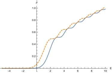
(a) $E^{\prime}=-3$

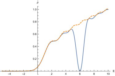
(b) $E^{\prime}=6$

Figure 5: Plot of $\widetilde{\rho}(E,E^{\prime})$ in (226) for 5(a) $E^{\prime}=-3$ and 5(b) $E^{\prime}=6$, as a function of $E$. The solid curves are the deformed eigenvalue density $\widetilde{\rho}(E,E^{\prime})$ while the orange dashed curve represents the original eigenvalue density $\widetilde{\rho}(E)=K(-E,-E)$ without FZZT branes.

6.3 Spectral form factor in FZZT brane background

Let us consider the two-point function of macroscopic loops in the presence of two FZZT branes

$$g(\beta_{1},\beta_{2},\xi) =\frac{\langle Z(\beta_{1})Z(\beta_{2})\Psi(\xi)^{2}\rangle}{\langle\Psi(\xi)^{2}\rangle}.$$ (227)

As in the previous subsection, we put two FZZT branes since single FZZT brane is not positive definite. From our general formula (203) we find

$$g(\beta_{1},\beta_{2},\xi) =\langle Z(\beta_{1})Z(\beta_{2})\rangle$$ (228)

$$+\frac{1}{K(\xi,\xi)}\Biggl{[}-\langle\xi|\Pi e^{(\beta_{1}+\beta_{2})Q}\Pi|\xi\rangle+2\langle\xi|\Pi e^{\beta_{1}Q}\Pi e^{\beta_{2}Q}\Pi|\xi\rangle$$

$$\qquad\qquad-\langle Z(\beta_{1})\rangle\langle\xi|\Pi e^{\beta_{2}Q}\Pi|\xi\rangle-\langle Z(\beta_{2})\rangle\langle\xi|\Pi e^{\beta_{1}Q}\Pi|\xi\rangle\Biggr{]}.$$

We can show that this is rewritten as

$$g(\beta_{1},\beta_{2},\xi) =\int d\lambda e^{(\beta_{1}+\beta_{2})\lambda}\frac{1}{K(\xi,\xi)}\left|\begin{matrix}K(\lambda,\lambda)&K(\lambda,\xi)\\ K(\xi,\lambda)&K(\xi,\xi)\end{matrix}\right|$$ (229)

$$+\int\prod_{i=1}^{2}d\lambda_{i}e^{\beta_{i}\lambda_{i}}\frac{1}{K(\xi,\xi)}\left|\begin{matrix}K(\lambda_{1},\lambda_{1})&K(\lambda_{1},\lambda_{2})&K(\lambda_{1},\xi)\\ K(\lambda_{2},\lambda_{1})&K(\lambda_{2},\lambda_{2})&K(\lambda_{2},\xi)\\ K(\xi,\lambda_{1})&K(\xi,\lambda_{2})&K(\xi,\xi)\end{matrix}\right|.$$

We consider the spectral form factor (SFF) in the presence of two FZZT branes $\Psi(\xi)^{2}$ at $\xi=-E^{\prime}$

$$\widetilde{g}(t,\beta,E^{\prime})=g(\beta+\mathrm{i}t,\beta-\mathrm{i}t,-E^{\prime}).$$ (230)

Using the CD kernel for the Airy case (221) and the integral representation (229), we can evaluate this SFF (230) numerically. In Figure 6 we show the plot of SFF in the Airy case with two FZZT branes for $\beta=1/100$ with several different values of $E^{\prime}$. For $E^{\prime}=-3$ and $E^{\prime}=3$, we do not see a notable deviation from the original SFF without the FZZT branes (orange dashed curve in Figure 6), but the $E^{\prime}=20$ case in Figure 6(c) has some oscillatory behavior. As discussed in Blommaert:2019wfy , we expect that the erratic behavior arises if we put many FZZT branes. It is tempting to speculate that the oscillatory behavior in Figure 6(c) might be an indication towards the erratic behavior as we increase the number of FZZT branes. It would be interesting to study the SFF with many FZZT brane insertions explicitly in the Airy case. However, this is a challenging problem since the generalization of (229) for many FZZT brane insertions is a multi-variable integral which is not easy to evaluate numerically with high precision. We leave this as an interesting future problem.

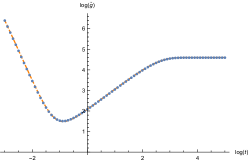
(a) $E^{\prime}=-3$

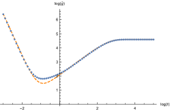
(b) $E^{\prime}=3$

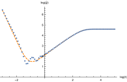
(c) $E^{\prime}=20$

Figure 6: Plot of SFF $\widetilde{g}(t,\beta,E^{\prime})$ with $\beta=1/100$ for 6(a) $E^{\prime}=-3$, 6(b) $E^{\prime}=3$ and 6(c) $E^{\prime}=20$ as a function of $t$. The blue dots represent the SFF in the presence of two FZZT branes at $\xi=-E^{\prime}$, while the orange dashed curve represents the SFF without the FZZT branes.

7 Conclusions and outlook

In this paper we have studied FZZT branes in JT gravity and topological gravity. We found that FZZT branes can be introduced in the matrix model of JT gravity Saad:2019lba by attaching $\mathcal{M}(b)=-e^{-zb}$ to the geodesic boundary of length $b$ and integrating over $b$ (see Figure 1). Our construction can be generalized to arbitrary background $\{t_{k}\}$ of topological gravity by introducing the generalized WP volume (37). We argued that the trumpet ending on a FZZT brane can be thought of as a “half-wormhole” introduced in Saad:2021rcu (see Figure 2). We found that the half-wormhole amplitude is given by the complementary error function (57). FZZT branes induce the shift of couplings (42) which is consistent with the known property of BA function in the literature. However, the expression such as (133) only gives an asymptotic expansion of the BA function in a certain sector of the complex $z$-plane (19). In section 5 we found the general formulae (203) and (204) for the generating function of the correlator of FZZT branes and macroscopic loops. Our formula expresses the correlator of FZZT branes and macroscopic loops in terms of the BA function and the CD kernel, which in principle can be defined non-perturbatively. As an example, in section 6 we studied the eigenvalue density and the spectral form factor (SFF) deformed by the insertion of two FZZT branes in the Airy case. In this explicit computation, we confirmed the picture of “eigenbranes” put forward in Blommaert:2019wfy .

There are many interesting open questions. It would be interesting to generalize our study of SFF by inserting more FZZT branes to see if we recover the erratic behavior of SFF as anticipated in Blommaert:2019wfy . Another interesting direction is the derivation of the Page curve in our formalism of FZZT branes. In Penington:2019kki , it is argued that the Page curve is reproduced by adding EOW brane degrees of freedom to JT gravity. As we have seen in (27), the EOW brane in Gao:2021uro is a special case of our formalism, corresponding to an infinite collection of anti-FZZT branes. It would be interesting to apply our formalism of FZZT branes to this problem. We should also mention that as argued in Maldacena:2004sn the “meson” field $S$ constructed out of the fermions in (12)

$$S_{ij}=\overline{\chi}_{ia}\chi_{aj}$$ (231)

can be identified as the matrix appearing in the Kontsevich model

$$e^{F(\bm{t})} =\int dSe^{\frac{\mathrm{i}}{2g_{\rm s}}\operatorname{Tr}\left(\frac{S^{3}}{3}+ZS^{2}\right)},$$ (232)

$$t_{k} =-g_{\rm s}(2k-1)!!\operatorname{Tr}Z^{-2k-1}.$$

It would be interesting to study, say, the second Rényi entropy

$$e^{-S_{2}}=\frac{\langle\operatorname{Tr}S^{2}\rangle}{\langle\operatorname{Tr}S\rangle^{2}}$$ (233)

in Kontsevich model in the JT gravity background with FZZT branes (81) to see if the Page curve is recovered. We leave this as an interesting future problem.

Appendix A $(2,p)$ minimal model background

The background for the $(2,p)$ minimal string is given by Mertens:2020hbs ; Turiaci:2020fjj

$$t_{k}-\delta_{k,1} =\frac{(-1)^{k}(m+k-2)!}{(k-1)!(m-k)!}\left(\frac{2}{2m-1}\right)^{2k-2},$$ (234)

where $p$ and $m$ are related by $p=2m-1$. One can see that $t_{k}$ in (234) reduces to $\gamma_{k}$ in (28) in the limit $m\to\infty$. In this sense, JT gravity is a $p\to\infty$ limit of the $(2,p)$ minimal string theory.

The Itzykson-Zuber variable $I_{0}$ for the minimal model background is

$$I_{0}(u)-u =\sum_{k=1}^{m}(t_{k}-\delta_{k,1})\frac{u^{k}}{k!}$$ (235)

$$=\frac{p}{8}\left[P_{m}\left(1-\frac{8u}{p^{2}}\right)-P_{m-2}\left(1-\frac{8u}{p^{2}}\right)\right],$$

where $P_{m}(x)$ denotes the Legendre polynomial.

The genus-zero eigenvalue density is given by

$$\rho_{0}(E) =\frac{1}{\pi g_{\rm s}}\sum_{k=1}^{m}\frac{(-1)^{k}(t_{k}-\delta_{k,1})}{(2k-1)!!}(2E)^{k-\frac{1}{2}}$$ (236)

$$=\frac{1}{\sqrt{2}\pi g_{\rm s}}\sinh\left[p\,\text{arcsinh}\left(\frac{2\sqrt{E}}{p}\right)\right],$$

and the disk amplitude is given by

$$\langle Z(\beta)\rangle^{g=0} =\frac{1}{\sqrt{2\pi}g_{\rm s}}\sum_{k=1}^{m}(-1)^{k}(t_{k}-\delta_{k,1})\beta^{-k-\frac{1}{2}}$$ (237)

$$=\frac{1}{\sqrt{2}\pi g_{\rm s}}\frac{p}{2\beta}e^{\frac{\beta p^{2}}{8}}K_{\frac{p}{2}}\Bigl{(}\frac{\beta p^{2}}{8}\Bigr{)}.$$

One can easily see that in the $p\to\infty$ limit the eigenvalue density of the $(2,p)$ minimal string (236) reduces to the eigenvalue density of JT gravity in (85).

Appendix B $Z(\beta)$-FZZT amplitude from inverse determinant

We can reproduce the $Z(\beta)$-FZZT amplitude (176) using the relation

$$\left\langle\operatorname{Tr}\frac{1}{x-M}\det(\xi-M)\right\rangle=\lim_{y\to x}\partial_{y}\left\langle\frac{\det(y-M)\det(\xi-M)}{\det(x-M)}\right\rangle.$$ (238)

The correlator of determinants and inverse determinants is studied in Fyodorov:2002jw ; Strahov:2002zu ; Baik_2003 . Using the result of Fyodorov:2002jw ; Strahov:2002zu ; Baik_2003 , we find

$$\left\langle\frac{\det(y-M)\det(\xi-M)}{\det(x-M)}\right\rangle=\frac{1}{\xi-y}\frac{1}{h_{N-1}}\left|\begin{matrix}\varphi_{N-1}(x)&\varphi_{N}(x)&\varphi_{N+1}(x)\\ P_{N-1}(y)&P_{N}(y)&P_{N+1}(y)\\ P_{N-1}(\xi)&P_{N}(\xi)&P_{N+1}(\xi)\end{matrix}\right|,$$ (239)

where $\varphi_{N}(x)$ is the Hilbert transform of the orthogonal polynomial $P_{N}(x)$

$$\varphi_{N}(x)=\int d\lambda\frac{e^{-V(\lambda)}}{x-\lambda}P_{N}(\lambda).$$ (240)

Thus we find

$$\left\langle\operatorname{Tr}\frac{1}{x-M}\det(\xi-M)\right\rangle=\frac{1}{\xi-x}\frac{1}{h_{N-1}}\int d\lambda\frac{e^{-V(\lambda)}}{x-\lambda}\left|\begin{matrix}P_{N-1}(\lambda)&P_{N}(\lambda)&P_{N+1}(\lambda)\\ P_{N-1}^{\prime}(x)&P_{N}^{\prime}(x)&P_{N+1}^{\prime}(x)\\ P_{N-1}(\xi)&P_{N}(\xi)&P_{N+1}(\xi)\end{matrix}\right|+\frac{P_{N}(\xi)}{\xi-x}.$$ (241)

By using the relation

$$\lambda P_{N}(\lambda)=P_{N+1}(\lambda)+\frac{h_{N}}{h_{N-1}}P_{N-1}(\lambda),$$ (242)

the first term of (241) is written as

$$\frac{1}{\xi-x}\frac{1}{h_{N-1}}\int d\lambda\frac{e^{-V(\lambda)}}{x-\lambda}\left|\begin{matrix}P_{N-1}(\lambda)&P_{N}(\lambda)&\lambda P_{N}(\lambda)\\ P_{N-1}^{\prime}(x)&P_{N}^{\prime}(x)&xP_{N}^{\prime}(x)+P_{N}(x)\\ P_{N-1}(\xi)&P_{N}(\xi)&\xi P_{N}(\xi)\end{matrix}\right|$$ (243)

$$=\frac{1}{\xi-x}\frac{1}{h_{N-1}}\int d\lambda\frac{e^{-V(\lambda)}}{x-\lambda}\left|\begin{matrix}P_{N-1}(\lambda)&P_{N}(\lambda)&(\lambda-x)P_{N}(\lambda)\\ P_{N-1}^{\prime}(x)&P_{N}^{\prime}(x)&P_{N}(x)\\ P_{N-1}(\xi)&P_{N}(\xi)&(\xi-x)P_{N}(\xi)\end{matrix}\right|$$

$$=\frac{1}{h_{N-1}}\int d\lambda\frac{e^{-V(\lambda)}}{x-\lambda}\Biggl{[}P_{N}(\xi)\Bigl{(}P_{N-1}(\lambda)P_{N}^{\prime}(x)-P_{N}(\lambda)P_{N-1}^{\prime}(x)\Bigr{)}$$

$$\quad-P_{N}(x)\frac{P_{N-1}(\lambda)P_{N}(\xi)-P_{N}(\lambda)P_{N-1}(\xi)}{\xi-x}\Biggr{]}.$$

In the last equality we used the orthogonality relation (114). Let us consider the first half of (243)

$$\frac{1}{h_{N-1}}\int d\lambda\frac{e^{-V(\lambda)}}{x-\lambda}P_{N}(\xi)\Bigl{(}P_{N-1}(\lambda)P_{N}^{\prime}(x)-P_{N}(\lambda)P_{N-1}^{\prime}(x)\Bigr{)}$$ (244)

$$=\frac{1}{h_{N-1}}\int d\lambda\frac{e^{-V(\lambda)}}{x-\lambda}P_{N}(\xi)\Bigl{(}P_{N-1}(\lambda)P_{N}^{\prime}(\lambda)-P_{N}(\lambda)P_{N-1}^{\prime}(\lambda)\Bigr{)}$$

$$\quad+\frac{P_{N}(\xi)}{h_{N-1}}\int d\lambda e^{-V(\lambda)}\Biggl{[}P_{N-1}(\lambda)\frac{P_{N}^{\prime}(x)-P_{N}^{\prime}(\lambda)}{x-\lambda}-P_{N}(\lambda)\frac{P_{N-1}^{\prime}(x)-P_{N-1}^{\prime}(\lambda)}{x-\lambda}\Biggr{]}$$

$$=\frac{1}{h_{N-1}}\int d\lambda\frac{e^{-V(\lambda)}}{x-\lambda}P_{N}(\xi)\Bigl{(}P_{N-1}(\lambda)P_{N}^{\prime}(\lambda)-P_{N}(\lambda)P_{N-1}^{\prime}(\lambda)\Bigr{)}.$$

In the last step we used the orthogonality relation (114). The second half of (243) is

$$\frac{1}{h_{N-1}}\int d\lambda\frac{e^{-V(\lambda)}}{x-\lambda}P_{N}(x)\frac{P_{N-1}(\lambda)P_{N}(\xi)-P_{N}(\lambda)P_{N-1}(\xi)}{x-\xi}$$ (245)

$$= \frac{1}{h_{N-1}}\int d\lambda e^{-V(\lambda)}\frac{P_{N}(x)-P_{N}(\lambda)+P_{N}(\lambda)}{x-\lambda}\frac{P_{N-1}(\lambda)P_{N}(\xi)-P_{N}(\lambda)P_{N-1}(\xi)}{x-\xi}.$$

Using the relation

$$\frac{P_{N}(x)-P_{N}(\lambda)}{x-\lambda}=P_{N-1}(\lambda)+(\text{lower degree terms in}~{}\lambda)$$ (246)

(245) becomes

$$\frac{P_{N}(\xi)}{x-\xi}+\frac{1}{h_{N-1}}\int d\lambda e^{-V(\lambda)}\frac{P_{N}(\lambda)}{x-\lambda}\frac{P_{N-1}(\lambda)P_{N}(\xi)-P_{N}(\lambda)P_{N-1}(\xi)}{x-\xi}$$ (247)

$$= \frac{P_{N}(\xi)}{x-\xi}+\frac{1}{h_{N-1}}\int d\lambda e^{-V(\lambda)}\left(\frac{1}{x-\xi}-\frac{1}{x-\lambda}\right)P_{N}(\lambda)\frac{P_{N-1}(\lambda)P_{N}(\xi)-P_{N}(\lambda)P_{N-1}(\xi)}{\xi-\lambda}$$

$$= \frac{P_{N}(\xi)}{x-\xi}-\frac{1}{h_{N-1}}\int d\lambda e^{-V(\lambda)}\frac{P_{N}(\lambda)}{x-\lambda}\frac{P_{N-1}(\lambda)P_{N}(\xi)-P_{N}(\lambda)P_{N-1}(\xi)}{\xi-\lambda}.$$

The first term cancels out the last term of (241). Finally we find

$$\left\langle\operatorname{Tr}\frac{1}{x-M}\det(\xi-M)\right\rangle=\frac{1}{h_{N-1}}\int d\lambda\frac{e^{-V(\lambda)}}{x-\lambda}\Biggl{[}P_{N}(\xi)\Bigl{(}P_{N}^{\prime}(\lambda)P_{N-1}(\lambda)-P_{N}(\lambda)P_{N-1}^{\prime}(\lambda)\Bigr{)}$$ (248)

$$-P_{N}(\lambda)\frac{P_{N}(\xi)P_{N-1}(\lambda)-P_{N-1}(\xi)P_{N}(\lambda)}{\xi-\lambda}\Biggr{]}.$$

In the double scaling limit this becomes

$$\left\langle\operatorname{Tr}\frac{1}{x-M}\Psi(\xi)\right\rangle=\int\frac{d\lambda}{x-\lambda}\Bigl{[}K(\lambda,\lambda)\psi(\xi)-K(\xi,\lambda)\psi(\lambda)\Bigr{]}.$$ (249)

This reproduces the deformed eigenvalue density due to the insertion of one FZZT brane in (176).

One can in principle derive the multi-point correlator of $Z(\beta)$’s and FZZT branes in this approach using the result in Fyodorov:2002jw ; Strahov:2002zu ; Baik_2003 . We leave this as an interesting future problem.

References

- (1) R. Jackiw, “Lower Dimensional Gravity,” Nucl. Phys. B252 (1985) 343–356.
- (2) C. Teitelboim, “Gravitation and Hamiltonian Structure in Two Space-Time Dimensions,” Phys. Lett. 126B (1983) 41–45.
- (3) P. Saad, S. H. Shenker, and D. Stanford, “JT gravity as a matrix integral,” arXiv:1903.11115 [hep-th].
- (4) A. Blommaert, T. G. Mertens, and H. Verschelde, “Eigenbranes in Jackiw-Teitelboim gravity,” JHEP 02 (2021) 168, arXiv:1911.11603 [hep-th].
- (5) V. Fateev, A. B. Zamolodchikov, and A. B. Zamolodchikov, “Boundary Liouville field theory. 1. Boundary state and boundary two point function,” arXiv:hep-th/0001012.
- (6) J. Teschner, “Remarks on Liouville theory with boundary,” PoS tmr2000 (2000) 041, arXiv:hep-th/0009138.
- (7) G. Penington, S. H. Shenker, D. Stanford, and Z. Yang, “Replica wormholes and the black hole interior,” arXiv:1911.11977 [hep-th].
- (8) P. Gao, D. L. Jafferis, and D. K. Kolchmeyer, “An effective matrix model for dynamical end of the world branes in Jackiw-Teitelboim gravity,” arXiv:2104.01184 [hep-th].
- (9) A. Goel, L. V. Iliesiu, J. Kruthoff, and Z. Yang, “Classifying boundary conditions in JT gravity: from energy-branes to -branes,” JHEP 04 (2021) 069, arXiv:2010.12592 [hep-th].
- (10) P. Saad, S. H. Shenker, D. Stanford, and S. Yao, “Wormholes without averaging,” arXiv:2103.16754 [hep-th].
- (11) K. Okuyama and K. Sakai, “JT gravity, KdV equations and macroscopic loop operators,” JHEP 01 (2020) 156, arXiv:1911.01659 [hep-th].
- (12) D. Kutasov, K. Okuyama, J.-w. Park, N. Seiberg, and D. Shih, “Annulus amplitudes and ZZ branes in minimal string theory,” JHEP 08 (2004) 026, arXiv:hep-th/0406030.
- (13) J. M. Maldacena, G. W. Moore, N. Seiberg, and D. Shih, “Exact vs. semiclassical target space of the minimal string,” JHEP 10 (2004) 020, arXiv:hep-th/0408039.
- (14) M. Mulase and B. Safnuk, “Mirzakhani’s recursion relations, Virasoro constraints and the KdV hierarchy,” arXiv:math/0601194 [math].
- (15) R. Dijkgraaf and E. Witten, “Developments in Topological Gravity,” Int. J. Mod. Phys. A 33 no. 30, (2018) 1830029, arXiv:1804.03275 [hep-th].
- (16) E. Witten, “Two-dimensional gravity and intersection theory on moduli space,” Surveys Diff. Geom. 1 (1991) 243–310.
- (17) M. Kontsevich, “Intersection theory on the moduli space of curves and the matrix Airy function,” Commun. Math. Phys. 147 (1992) 1–23.
- (18) G. W. Moore, N. Seiberg, and M. Staudacher, “From loops to states in 2-D quantum gravity,” Nucl. Phys. B362 (1991) 665–709.
- (19) K. Okuyama and K. Sakai, “Multi-boundary correlators in JT gravity,” JHEP 08 (2020) 126, arXiv:2004.07555 [hep-th].
- (20) E. Date, M. Jimbo, M. Kashiwara, and T. Miwa, “Transformation groups for soliton equations.: Euclidean Lie algebras and reduction of the KP hierarchy,” Publ. Res. Inst. Math. Sci. Kyoto 18 no. 3, (1982) 1077–1110.
- (21) M. Bertola, B. Dubrovin, and D. Yang, “Correlation functions of the KdV hierarchy and applications to intersection numbers over ,” Physica D 327 (2016) 30–57, arXiv:1504.06452 [math-ph].
- (22) J. Lepowsky and R. L. Wilson, “Construction of the Affine Lie Algebra A1(1),” Commun. Math. Phys. 62 (1978) 43–53.
- (23) E. Date, M. Kashiwara, and T. Miwa, “TRANSFORMATION GROUPS FOR SOLITON EQUATIONS. 2. VERTEX OPERATORS AND tau FUNCTIONS,” Proc. Jap. Acad. A 57 (1981) 387–392.
- (24) N. Seiberg and D. Shih, “Branes, rings and matrix models in minimal (super)string theory,” JHEP 02 (2004) 021, arXiv:hep-th/0312170.
- (25) N. Seiberg and D. Shih, “Minimal string theory,” Comptes Rendus Physique 6 (2005) 165–174, arXiv:hep-th/0409306.
- (26) D. Gaiotto and L. Rastelli, “A Paradigm of open / closed duality: Liouville D-branes and the Kontsevich model,” JHEP 07 (2005) 053, arXiv:hep-th/0312196.
- (27) T. G. Mertens and G. J. Turiaci, “Liouville quantum gravity – holography, JT and matrices,” JHEP 01 (2021) 073, arXiv:2006.07072 [hep-th].
- (28) K. Okuyama and K. Sakai, “A proof of loop equations in 2d topological gravity,” arXiv:2106.05643 [hep-th].
- (29) C. Itzykson and J. B. Zuber, “Combinatorics of the modular group. 2. The Kontsevich integrals,” Int. J. Mod. Phys. A7 (1992) 5661–5705, arXiv:hep-th/9201001.
- (30) B. Mukhametzhanov, “Half-wormhole in SYK with one time point,” arXiv:2105.08207 [hep-th].
- (31) S. Choudhury and K. Shirish, “Wormhole calculus without averaging from tensor model,” arXiv:2106.14886 [hep-th].
- (32) A. M. García-García and V. Godet, “Half-wormholes in nearly AdS2 holography,” arXiv:2107.07720 [hep-th].
- (33) P. Saad, S. Shenker, and S. Yao, “Comments on wormholes and factorization,” arXiv:2107.13130 [hep-th].
- (34) A. Blommaert and J. Kruthoff, “Gravity without averaging,” arXiv:2107.02178 [hep-th].
- (35) P. H. Ginsparg and G. W. Moore, “Lectures on 2-D gravity and 2-D string theory,” in Theoretical Advanced Study Institute (TASI 92): From Black Holes and Strings to Particles. 10, 1993. arXiv:hep-th/9304011.
- (36) E. J. Martinec, “The Annular report on noncritical string theory,” arXiv:hep-th/0305148.
- (37) G. W. Moore and N. Seiberg, “From loops to fields in 2-D quantum gravity,” Int. J. Mod. Phys. A 7 (1992) 2601–2634.
- (38) D. Stanford and E. Witten, “Fermionic Localization of the Schwarzian Theory,” JHEP 10 (2017) 008, arXiv:1703.04612 [hep-th].
- (39) H. Maxfield and G. J. Turiaci, “The path integral of 3D gravity near extremality; or, JT gravity with defects as a matrix integral,” JHEP 01 (2021) 118, arXiv:2006.11317 [hep-th].
- (40) E. T. Whittaker and G. N. Watson, “A Course of Modern Analysis: 4th Edition (Cambridge Mathematical Library),” Cambridge University Press (1996) .
- (41) E. Witten, “Matrix Models and Deformations of JT Gravity,” Proc. Roy. Soc. Lond. A 476 no. 2244, (2020) 20200582, arXiv:2006.13414 [hep-th].
- (42) T. Budd, “Irreducible metric maps and Weil-Petersson volumes,” arXiv:2012.11318 [math-ph].
- (43) C. V. Johnson and F. Rosso, “Solving Puzzles in Deformed JT Gravity: Phase Transitions and Non-Perturbative Effects,” JHEP 04 (2021) 030, arXiv:2011.06026 [hep-th].
- (44) S. Forste, H. Jockers, J. Kames-King, and A. Kanargias, “Deformations of JT Gravity via Topological Gravity and Applications,” arXiv:2107.02773 [hep-th].
- (45) T. G. Mertens and G. J. Turiaci, “Defects in Jackiw-Teitelboim Quantum Gravity,” JHEP 08 (2019) 127, arXiv:1904.05228 [hep-th].
- (46) N. Seiberg and D. Starnford, “unpublished,”.
- (47) G. J. Turiaci, M. Usatyuk, and W. W. Weng, “Dilaton-gravity, deformations of the minimal string, and matrix models,” arXiv:2011.06038 [hep-th].
- (48) B. Eynard, T. Kimura, and S. Ribault, “Random matrices,” arXiv:1510.04430 [math-ph].
- (49) A. Morozov, “Integrability and matrix models,” Phys. Usp. 37 (1994) 1–55, arXiv:hep-th/9303139.
- (50) E. Brézin and S. Hikami, “Characteristic polynomials of random matrices,” Commun. Math. Phys. 214 (2000) 111–135, arXiv:math-ph/9910005.
- (51) K. Okuyama and K. Sakai, “JT supergravity and Brezin-Gross-Witten tau-function,” JHEP 10 (2020) 160, arXiv:2007.09606 [hep-th].
- (52) E. Strahov and Y. V. Fyodorov, “Universal results for correlations of characteristic polynomials: Riemann-Hilbert approach,” Commun. Math. Phys. 241 (2003) 343–382, arXiv:math-ph/0210010.
- (53) T. Banks, M. R. Douglas, N. Seiberg, and S. H. Shenker, “Microscopic and Macroscopic Loops in Nonperturbative Two-dimensional Gravity,” Phys. Lett. B238 (1990) 279.
- (54) K. Okuyama, “Connected correlator of 1/2 BPS Wilson loops in SYM,” JHEP 10 (2018) 037, arXiv:1808.10161 [hep-th].
- (55) A. Okounkov, “Generating functions for intersection numbers on moduli spaces of curves,” International Mathematics Research Notices 2002 no. 18, (2002) 933–957, arXiv:math/0101201 [math.AT].
- (56) Y. V. Fyodorov and E. Strahov, “An Exact formula for general spectral correlation function of random Hermitian matrices,” J. Phys. A 36 (2003) 3203–3214, arXiv:math-ph/0204051.
- (57) J. Baik, P. Deift, and E. Strahov, “Products and ratios of characteristic polynomials of random hermitian matrices,” J. Math. Phys. 44 (2003) 3657–3670, arXiv:math-ph/0304016.