EMPRESS. IV.
Extremely Metal-Poor Galaxies (EMPGs) Including Very Low-Mass
Primordial Systems with $M_{*}=10^{4}$–$10^{5}$ M_⊙ and 2–3% (O/H)_⊙:
High (Fe/O) Suggestive of Metal Enrichment by Hypernovae/Pair-Instability Supernovae

Abstract

We present Keck/LRIS follow-up spectroscopy for 13 photometric candidates of extremely metal poor galaxies (EMPGs) selected by a machine-learning technique applied to the deep ($\sim 26$ AB mag) optical and wide-area ($\sim 500$ deg²) Subaru imaging data in the EMPRESS survey. Nine out of the 13 candidates are EMPGs with an oxygen abundance (O/H) less than $\sim 10$% solar value (O/H)_⊙, and four sources are contaminants of moderately metal-rich galaxies or no emission-line objects. Notably, two out of the nine EMPGs have extremely-low stellar masses and oxygen abundances of $5\times 10^{4}$–$7\times 10^{5}$ M_⊙ and 2–3% (O/H)_⊙, respectively. With a sample of five EMPGs with (Fe/O) measurements, two (three) of which are taken from this study (the literature), we confirm that two EMPGs with the lowest (O/H) ratios of $\sim 2$% (O/H)_⊙ show high (Fe/O) ratios of $\sim 0.1$, close to the solar abundance ratio. Comparing galaxy chemical enrichment models, we find that the two EMPGs cannot be explained by a scenario of metal-poor gas accretion/episodic star-formation history due to their low (N/O) ratios. We conclude that the two EMPGs can be reproduced by an inclusion of bright hypernovae and/or hypothetical pair-instability supernovae (SNe) preferentially produced in a metal-poor environment. This conclusion implies that primordial galaxies at $z\sim 10$ could have a high abundance of Fe that is not originated from Type Ia SNe with delays, and that Fe may not serve as a cosmic clock for primordial galaxies.

1 Introduction

Galaxies in the early formation phase are the keys to understanding galaxy formation and evolution. Young galaxies, especially galaxies with stellar ages below $\sim 300$ Myr, are expected to be metal-poor, because low- and intermediate-mass stars cannot contribute to chemical enrichment before finishing lifetimes of $\sim 300$ Myr as main-sequence stars. Wise et al. (2012) predict that a first galaxy at $z\gtrsim 7$ (corresponding to the stellar age of $\lesssim 300$ Myr) has a halo mass of $10^{7}$–$10^{9}$ M_⊙, a stellar mass of $10^{4}$–$10^{6}$ M_⊙, and a metallicity of 0.1–1% solar abundance.

In such an extremely low-metallicity environment, progenitor gas clouds of stars are also metal-poor. The metal-poor gas cools less efficiently than metal-rich gas because metals are much more efficient coolants than hydrogen. In such a metal-poor and high-temperature environment, protostellar cores exhibit large Jeans masses, consequently evolving into massive stars. Performing cosmological zoom-in simulations, Hirano et al. (2015) obtain $\sim 300$ M_⊙ stars in primordial star-forming clouds. Hirano et al. (2015) also report the mass distribution of first stars, which is indicative that very massive ($\gtrsim 100$ M_⊙) stars are born in the metal-free environment.

Metal-poor (and thus young) galaxies potentially undergo chemical evolutions largely affected by massive stars. Especially, iron-to-oxygen (Fe/O) abundance ratios strongly depend on galaxy ages and initial mass functions (IMFs) because stars with different masses undergo different types of supernova (SN) explosions ejecting different amount of iron and oxygen (Section 6.1). If we calculate ejecta from Type Ia SNe and core-collapse SNe (CCSNe) only, the Fe/O ratio monotonically increases with age (and thus can serve as a cosmic clock; Xing et al. 2019). Before the appearance of Type Ia SNe, however, high Fe/O gas can also be produced by hypernovae (HNe) and pair-instability SNe (PISNe), whose progenitor stars are more massive than $\sim 30$ and 200 M_⊙, respectively. Extremely-young metal-poor galaxies may have high Fe/O ratios because both HNe and PISNe tend to be produced in metal-poor environments. Now we should evaluate the HN or PISN contributions to Fe/O in the early galaxy formation phase to test whether Fe/O can truly act as a cosmic clock in primordial galaxies.

We can verify whether HNe and/or PISNe play important roles in the Fe/O evolution of galaxies by observing extremely young ($\lesssim 10$ Myr) galaxies. However, such galaxies are intrinsically too faint because of their low stellar masses. Assuming $M_{*}=10^{6}$ M_⊙ (Wise et al., 2012) and the large rest-frame equivalent width of EW₀(H$\alpha)=3700$ Å under the assumptions of the age of 1 Myr, metal free, and constant star formation (Inoue, 2011), we derive the H$\alpha$ flux of extremely-young low-mass galaxy at each redshift. As illustrated in Figure 1, the expected H$\alpha$ fluxes of the young low-mass galaxies (black) is $>1$ dex smaller than the limiting fluxes of the current-best instruments of Keck/LRIS and Keck/MOSFIRE within the redshift range of $z\gtrsim 0.5$. Even using the forthcoming Thirty Meter Telescope (TMT) and James Webb Space Telescope (JWST), we can detect H$\alpha$ of the young low-mass galaxies only at $z\lesssim 2$. This means that it is difficult to detect young galaxies having $M_{*}\lesssim 10^{6}\ {\rm M}_{\odot}$ at $z\gtrsim 2$ even with the forthcoming large telescopes without gravitational lensing (e.g., Kikuchihara et al. 2020).

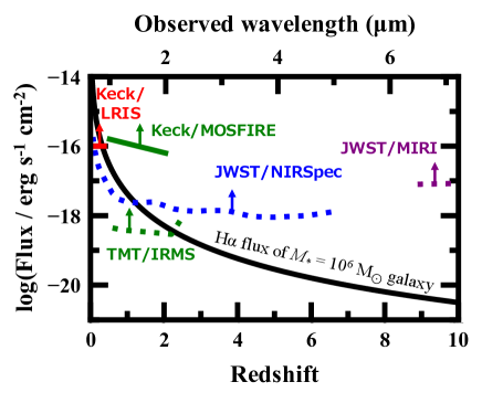
Figure 1: Expected H$\alpha$ flux of young galaxies with $M_{*}=10^{6}$ M_⊙ and EW₀(H$\alpha)=3700$ Å at a given redshift (black solid curve). The red and green solid lines indicate the limiting fluxes of the current-best instruments of Keck/LRIS and Keck/MOSFIRE, respectively. The green, blue, and purple dotted lines represent the limiting fluxes of the near-future instruments of TMT/IRMS, JWST/NIRSpec, and JWST/MIRI, respectively. These limiting fluxes are calculated under the assumption that a point source has an emission line that should be detected at a signal-to-noise ratio of 10 in an exposure time of 10000 second. The limiting fluxes of the instruments of TMT and JWST are derived from Hees et al. (2015) and Gardner et al. (2006), respectively.

Complementing these high-$z$ galaxy observations, various studies actively investigate local young dwarf galaxies (e.g., Berg et al., 2019). Although characteristics and formation processes of local young galaxies would be different from high-$z$ galaxies (Isobe et al. 2021; hereafter Paper III), local young galaxies are useful not only for studying galaxies at the early-formation stage, but also for understanding local young galaxies themselves, as living fossils of forming galaxies in the universe today. Although such low-mass and metal-poor galaxies become rarer toward lower redshifts (Behroozi et al., 2013; Morales-Luis et al., 2011), recent studies show the presence of extremely metal-poor galaxies (EMPGs; defined as galaxies with $\leq 12+\log(\rm O/H)=7.69=10$% (O/H)_⊙) in the local universe such as SBS0335$-$052 (Izotov et al., 2009), AGC198691 (Hirschauer et al., 2016), J1234+3901 (Izotov et al., 2019), Little Cub (Hsyu et al., 2017), DDO68 (Pustilnik et al., 2005), and IZw18 (Izotov & Thuan, 1998). A blind H i survey (ALFALFA) has identified Leo P with $\sim 3$% (O/H)_⊙ (Skillman et al., 2013). Significant progress has been made recently with EMPG spectroscopic and photometric samples of Sloan Digital Sky Survey (SDSS). Sánchez Almeida et al. (2016) have found 196 EMPGs from the SDSS spectroscopic data, and Izotov et al. (2018) have identified J0811+4730 with a metallicity down to 2% (O/H)_⊙. The SDSS imaging data have largely contributed to identify many EMPGs (e.g., James et al., 2015, 2017; Hsyu et al., 2018; Senchyna & Stark, 2019).

However, such previous studies based on SDSS are not ideal for pinpointing low-mass (and thus faint) EMPGs due to their shallow data. Kojima et al. (2020; hereafter Paper I) have launched a project entitled “Extremely Metal-Poor Representatives Explored by the Subaru Survey (EMPRESS)” with Subaru/Hyper Suprime-Cam (HSC) optical wide (500 deg²) and deep (5$\sigma$ limiting magnitude of $i_{\rm lim}=26$) images that are about 100 times deeper than those of SDSS (Aihara et al., 2019). EMPRESS has identified J1631+4426, whose metallicity is 1.6% (O/H)_⊙. J1631+4426 shows the lowest metallicity reported so far, with a low stellar mass of $\sim 10^{6}$ ${\rm M}_{\odot}$.

While J1631+4426 (Paper I) and J0811+4730 (Izotov et al., 2018) have extremely low-metallicities of $\sim 2$% (O/H)_⊙, Kojima et al. (2021; hereafter Paper II) have reported that the 2 EMPGs show high Fe/O ratios of $\sim(\rm Fe/O)_{\odot}$. Paper II concludes that the 2 EMPGs are too young to be affected by chemical enrichment of low- and intermediate-mass stars because the EMPGs have low N/O ratios. Alternatively, Paper II suggests that super-massive stars may contribute to the Fe/O enhancements, while the contribution has not been evaluated quantitatively.

This paper is the fourth paper of EMPRESS, reporting spectroscopic follow-up observations for the remaining EMPG candidates with Keck Telescope. We also derive chemical properties of the EMPGs including $12+\log(\rm O/H)$ and Fe/O to discuss chemical enrichment of galaxies in the early formation phase. We present the EMPG sample in Section 2. In Section 3 we explain our optical spectroscopy and data reductions. We explain our data analysis in Section 4. We report and discuss chemical properties of EMPGs in Section 5. We discuss further the origin of the Fe/O enhancements of the EMPGs in Section 6. Section 7 summarizes our findings. Throughout this paper, magnitudes are in the AB system (Oke & Gunn, 1983), and we assume a standard $\Lambda$CDM cosmology with parameters of ($\Omega_{\rm m}$, $\Omega_{\rm\Lambda}$, $H_{0}$) = (0.3, 0.7, 70 km ${\rm s}^{-1}$ ${\rm Mpc}^{-1}$). The definition of solar metallicity ${\rm Z}_{\odot}$ is given by $12+\log(\rm O/H)=8.69$ (Asplund et al., 2021). Solar abundance ratios of log(Ne/O), log(Ar/O), log(N/O), log(Fe/O) are $-0.63$, $-2.31$, $-0.86$, and $-1.23$, respectively (Asplund et al., 2021).

2 Sample

We use a photometric sample of EMPG candidates selected by Paper I. The Paper-I photometric sample consists of EMPG candidates identified from the data of HSC and SDSS, which we refer to as HSC EMPG candidates and SDSS EMPG candidates, respectively. In this paper, we do not use SDSS EMPG candidates, because the SDSS EMPG candidates include more contaminants than the HSC EMPG candidates (Paper I). The catalog of the HSC EMPG candidates is developed with the HSC-SSP S17A and S18A data (Aihara et al., 2019), which are wide and deep enough to search for rare and faint EMPGs. The HSC EMPG candidates are selected from $\sim 46$ million sources whose photometric measurements are brighter than 5$\sigma$ limiting magnitudes in all of the 4 broadbands, $g<26.5$, $r<26.0$, $i<25.8$, and $z<25.2$ mag (Ono et al., 2018), which correspond to absolute magnitudes at $z=0.03$ of $M_{g}<-9.1$, $M_{r}<-9.6$, $M_{i}<-9.8$, and $M_{z}<-10.4$ mag, respectively. The catalog consisting of these sources is referred to as the HSC source catalog.

With the HSC source catalog, Paper I isolates EMPGs from contaminants such as other types of galaxies, Galactic stars, and quasi-stellar objects (QSOs). Paper I aims to find galaxies at $z\leq 0.03$ with ${\rm EW}_{0}({\rm H}\alpha)>800$ Å and $12+\log{(\rm O/H)}=6.69$–7.69. Because it is difficult to distinguish EMPGs from the contaminants on 2-color diagrams such as $r-i$ vs. $g-r$, Paper I constructs a machine-learning classifier based on a deep neural network (DNN) with a training data set. The training data set is composed of mock photometric measurements for model spectra of EMPGs and the contaminants of other types of galaxies, Galactic stars, and QSOs. The DNN allows us to isolate EMPGs from the contaminants with non-linear boundaries in the multi-dimensional color space. Paper I finally obtains 27 HSC EMPG candidates from the HSC source catalog. Paper I conducts spectroscopic follow-up observations with Magellan/LDSS-3, Magellan/MagE, Keck/DEIMOS, and Subaru/FOCAS for 4 out of the 27 HSC EMPG candidates, and confirm that all of the 4 HSC EMPG candidates are truly emission-line galaxies with the low metallicity of $12+\log{(\rm O/H)}=6.90$–8.27 (i.e., 1.6–38% ${\rm Z}_{\odot}$). Paper I finds that 2 out of the 4 HSC EMPG candidates meet the EMPG criterion of $12+\log{(\rm O/H)}<7.69$ (i.e., $<10\%$ ${\rm Z}_{\odot}$). We refer to the 2 EMPGs as HSC spectroscopic EMPGs. There remain 23 ($=27-4$) HSC EMPG candidates that are not spectroscopically confirmed in Paper I. We refer to the 23 candidates as HSC photometric EMPGs.

3 Observations and Data Reduction

3.1 Spectroscopic Follow-up Observations with Keck/LRIS

Table 1: Coordinates of the HSC EMPG candidates

#	ID	R.A.	Dec.
		hh:mm:ss	dd:mm:ss
(1)	(2)	(3)	(4)
1	J0156$-$0421	01:56:51.6	$-$04:21:25.2
2	J0159$-$0622	01:59:43.8	$-$06:22:32.8
3	J0210$-$0124	02:10:12.0	$-$01:24:51.1
4	J0214$-$0243	02:14:24.3	$-$02:43:54.4
5	J0226$-$0517	02:26:57.6	$-$05:17:47.3
6	J0232$-$0248	02:32:13.3	$-$02:48:19.3
7	J1608$+$4337	16:08:11.0	+43:37:53.4
8	J2236$+$0444	22:36:12.4	+04:44:22.3
9	J2321$+$0125	23:21:52.2	+01:25:55.0
10	J2355$+$0200	23:55:30.1	+02:00:16.0
11	J0228$-$0256	02:28:36.3	$-$02:56:45.7
12	J2221$-$0015	22:21:26.1	$-$00:15:49.5
13	J2319$+$0136	23:19:33.6	+01:36:50.2

In this paper, we report spectroscopic observations with the Low Resolution Imaging Spectrograph (LRIS; Oke et al. 1995). LRIS is an imaging spectrometer installed at the Cassegrain focus of Keck Telescope, whose aperture area of is equivalent to that with a circular aperture of 9.96 m in diameter. LRIS has both blue and red channels that roughly cover wavelength ranges of 3000–6000 and 6000–10000 Å, respectively. LRIS can perform long-slit spectroscopy or multi-object spectroscopy (MOS).

We conducted spectroscopy with Keck/LRIS (PI: T. Kojima) for 13 out of the 23 HSC photometric EMPGs. The 13 targets were all the HSC photometric EMPGs observable at the observing night of 2019 August 31. Coordinates of the 13 HSC photometric EMPGs are listed in Table 1. We utilized the MOS mode and long-slit mode for 7 and 6 candidates, respectively. The slit widths were 1.5 arcsec for the all targets. We used the 600 lines mm^-1 grism blazed at 4000 Å on the blue channel and the 600 lines mm^-1 grating blazed at 7500 Å on the red channel. The LRIS spectroscopy of the blue and red channels covered the wavelength ranges of $\lambda\sim 3000$–5500 and 6000–9000 Å with the spectral resolutions of $\sim 4$ and 5 Å in FWHM, respectively. We also observed standard stars of a DOp-type star Feige 110 (RA=23:19:58.4, Dec.=$-$05:09:56 in J2000), a B2III-type star BD+40 4032 (RA=20:06:40.0, Dec.=+41:06:15 in J2000), and a B6V-type star Feige 25 (RA=02:36:00.0, Dec.=+05:15:17 in J2000). The sky was clear during the observations with seeing sizes of 0.8 arcsec. The observations are summarized in Table 1.

Figure 2 shows HSC images of the 13 HSC photometric EMPGs that we observed with LRIS. We note that many of the HSC photometric EMPGs (#2, 3, 4, 5, 6, 7, 9, 10, 11, and 13 in Figure 2) have diffuse structures (EMPG-tails; Paper III). We discuss the contribution of the EMPG-tails to the flux measurement of the HSC photometric EMPGs in Section 4.1.

[t] Summary of the LRIS observations # ID Mode Exposure sec (1) (2) (3) (4) 1 J0156$-$0421 Long slit 1200 2 J0159$-$0622 Long slit 1200 3 J0210$-$0124 MOS 1200 4 J0214$-$0243 MOS 1200 5 J0226$-$0517 MOS 1200 6 J0232$-$0248 MOS 1200 7 J1608$+$4337 MOS 1800 8 J2236$+$0444 Long slit 2400 9 J2321$+$0125 Long slit 3600 10 J2355$+$0200 MOS 2400 11^a J0228$-$0256 Long slit 1200 12^b J2221$-$0015 Long slit 2400 13^b J2319$+$0136 Long slit 600

• Contaminant: metal-rich galaxy (see Section 3.2)

• Contaminant: no emission line (see Section 3.2)

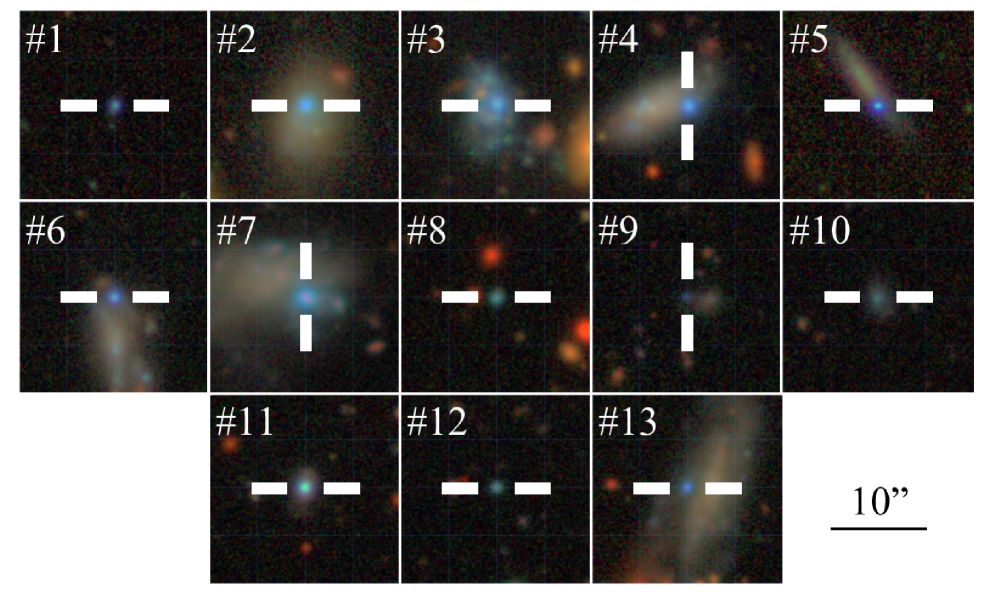
Figure 2: HSC $gri$-composite images of the 13 HSC photometric EMPGs that we observed with LRIS. The HSC $g$, $r$, and $i$-bands correspond to blue, green, and red colors in the figure, respectively. Each EMPG is located between the 2 white bars of each panel. The cut-out size is $20"\times 20"$. The number shown at the top left corner of each panel corresponds to the number in Table 1.

3.2 Data Reduction

To reduce and calibrate the data taken with LRIS, we use the iraf package. The reduction and calibration processes include the bias subtraction, flat fielding, cosmic ray cleaning, sky subtraction, wavelength calibration, one-dimensional (1D) spectrum extraction, flux calibration, atmospheric-absorption correction, and Galactic-reddening correction. The 1D spectra are derived from apertures centered on the blue compact component of the HSC photomeric EMPGs. We use the standard star Feige 110 for the flux calibration. The wavelengths are calibrated with the HgNeArCdZnKrXe lamp. We correct the atmospheric absorption with the extinction curve at Mauna Kea Observatories (Bèland et al., 1988). The Galactic-reddening value for each target is drawn from the NASA/IPAC Infrared Science Archive (IRSA) based on the Schlafly & Finkbeiner (2011) estimates.

We detect emission lines from 11 out of the 13 HSC photometric EMPGs. The remaining 2 HSC photometric EMPGs (J2221$-$0015 and J2319+0136; #12 and 13) with no emission line detected are probably contaminants, because the H$\alpha$ fluxes estimated from $r$-band excesses are $4\times 10^{-15}$–$1\times 10^{-14}$ erg s^-1 cm^-2, which should be detectable with the 10-minute exposure of LRIS. Figures 3 and 4 presents the reduced spectra of the 11 HSC photometric EMPGs. One out of the 11 HSC photometric EMPGs (J0228$-$0256; #11 in Figure 4) is located at $z=0.21$, which is out of the redshift range where Paper I aims to select EMPGs (Section 2). Because #11 shows a high [O ii]$\lambda\lambda$3727,3729/[O iii]$\lambda$5007 ratio and a strong Balmer break, #11 is likely to be a metal-rich galaxy. The remaining 10 HSC photometric EMPGs appear to be located at the redshifts of $z=0.009$–0.056, where Paper I aims to select EMPGs. Hereafter we refer to these 10 HSC photometric EMPGs as LRIS EMPG candidates. The inset panels of Figures 3 and 4 indicate that many of the LRIS EMPG candidates have emission lines with blue wings, suggestive of the outflow (Xu et al. in prep.; cf. Section 5.2).

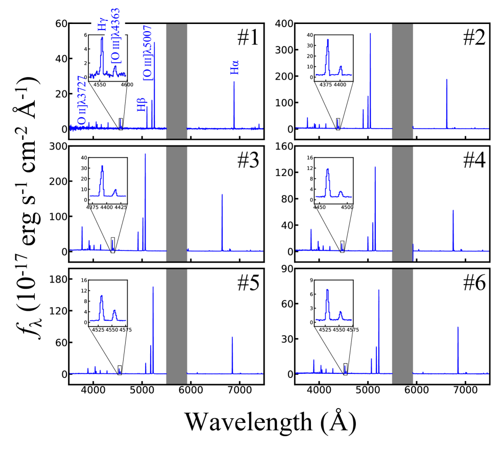
Figure 3: Reduced spectra of 6 out of the 11 HSC photometric EMPGs. The gray shaded regions indicate the gaps between the LRIS blue and red channels. The number shown at the top right corner of each panel corresponds to the number in Table 3. The inset panel at the top left corner of each panel illustrates an enlarged view of the spectrum around H$\gamma$ and [O iii]$\lambda$4363. The gray lines indicate errors of the spectra.

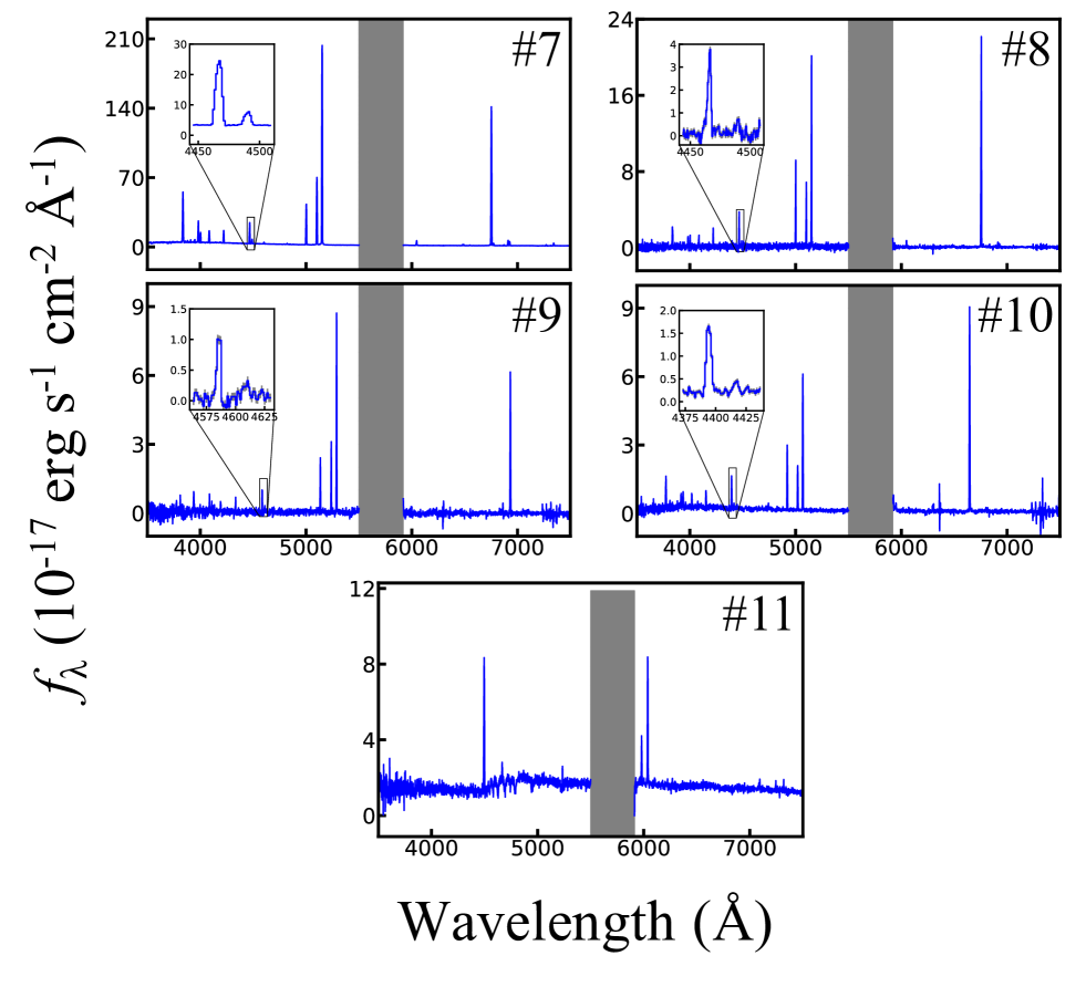
Figure 4: Reduced spectra of the remaining 5 of the 11 HSC photometric EMPGs. The symbols are the same as those in Figure 3. J0228$-$0256 (#11) is a metal-rich galaxy at $z=0.21$ (Section 3.2). The other 10 HSC photometric EMPGs are EMPG candidates at $z=0.009$–0.056.

4 Analysis

4.1 Flux Measurement

We measure central wavelengths, emission-line fluxes, and continua of the LRIS EMPG candidates (Section 3.2) with best-fit Gaussian (+ constant) profiles using the scipy.optimize package. We also estimate flux errors containing read-out noise and photon noise of sky and object emissions. None of the LRIS EMPG candidates show broad Balmer lines or high-ionization lines such as [Fe vii]$\lambda$6087, which suggests that the radiation from active galactic nuclei (AGNs) is not dominant in any LRIS EMPG candidate. We detect faint [O iii]$\lambda$4363 lines from all the 10 LRIS EMPG candidates. Because none of the LRIS EMPG candidates show [Fe ii]$\lambda$4288, whose flux is larger than that of [Fe ii]$\lambda$4359, the contamination of [O iii]$\lambda$4363 from [Fe ii]$\lambda$4359 is negligible. We also obtain very faint [Fe iii]$\lambda$4658 lines from 2 out of the 10 LRIS EMPG candidates (#2 and 7), which enables us to calculate Fe/O abundance ratios. This flux measurement probably represents an average of the whole galaxy because the size of the typical HSC EMPG is $\sim 0.3$ arcsec ($\sim 200$ pc; Paper III), which is smaller than the seeing size of 0.8 arcsec and the slit width of 1.5 arcsec. Redshifts are derived from the ratios between the observed central wavelengths and the rest-frame wavelengths in the air of H$\beta$ lines.

Color excesses $E(B-V)$ are derived from the Balmer decrement under the assumptions of the dust attenuation curve of Calzetti et al. (2000) and the case B recombination. We calculate $E(B-V)$, electron temperature $T_{\rm e}$, and electron density $n_{\rm e}$ iteratively so that all these properties are consistent with each other (see also Section 4.2). We obtain intrinsic values of Balmer emission-line ratios using PyNeb (Luridiana et al. 2015; v1.1.15). We derive $\chi^{2}$ of $E(B-V)$ from each Balmer emission-line ratio containing H$\alpha$, H$\beta$, H$\gamma$, and H$\delta$. Then, we find the best $E(B-V)$ values, which give the least $\chi^{2}$. We also obtain $\pm 68$% confidence intervals of $E(B-V)$ based on $\chi^{2}$. From all the LRIS EMPG candidates, we detect H$\gamma$ and H$\delta$ lines with ${\rm S/N}>13$ and ${\rm S/N}>5$, respectively. We also confirm that none of the H$\delta$, H$\gamma$, H$\beta$, and H$\alpha$ lines show significant stellar absorption. Using the $E(B-V)$ and the Calzetti et al. (2000) attenuation curve, we derive dust-corrected fluxes. We note that the dust-corrected fluxes are not very different from the observed ones, because most of the LRIS EMPG candidates show $E(B-V)\sim 0$ (i.e., dust-poor). The dust-corrected fluxes are summarized in Table 3. Again, we note that we detect the weak [Fe iii]$\lambda$4658 lines from 2 out of the 10 LRIS EMPG candidates, which are used to derive the Fe abundance. Other fundamental properties such as the redshift, rest-frame equivalent width of EW₀(H$\beta$), and $E(B-V)$ are listed in Table 4. Checking 2D spectra, we find that emission lines of EMPG-tails can contaminate those of EMPGs by at most 10%. We then add the uncertainties to lower errors of fluxes of EMPGs with EMPG-tails. On the other hand, stellar continua of EMPG-tails potentially contaminate those of EMPGs by at most 50%, which implies that EW₀(H$\beta$) of EMPGs would be underestimated. We calculate errors of EW₀(H$\beta$) including the uncertainties of stellar continua as well as those of H$\beta$ fluxes.

4.2 Chemical Property

Table 2: Atomic data

Ion	Emission process	Transition probability	Collision Strength
(1)	(2)	(3)	(4)
H0	Re	Storey & Hummer (1995)	—
O+	CE	Froese Fischer & Tachiev (2004)	Kisielius et al. (2009)
O2+	CE	Froese Fischer & Tachiev (2004)	Storey et al. (2014)
Ne2+	CE	Froese Fischer & Tachiev (2004)	McLaughlin & Bell (2000)
Ar2+	CE	Munoz Burgos et al. (2009)	Munoz Burgos et al. (2009)
N+	CE	Froese Fischer & Tachiev (2004)	Tayal (2011)
Fe2+	CE	Quinet (1996); Johansson et al. (2000)	Zhang (1996)

All of the LRIS EMPG candidates have [O iii]$\lambda$4363 detections, which allows us to derive metallicities and other element abundances with the direct-$T_{\rm e}$ method (e.g., Izotov et al., 2006) as described below.

The electron temperature $T_{\rm e}$ is calculated from two collisional excitation lines of the same ion such as O²⁺, because the collisional excitation rate is determined by $T_{\rm e}$. Using the PyNeb package getCrossTemDen with the latest atomic data and temperature relationship listed in Table 2, we derive $T_{\rm e}$ of O²⁺ ($T_{\rm e}$(O iii)) and $n_{\rm e}$ from emission-line ratios of [O iii]$\lambda$4363/[O iii]$\lambda\lambda$4959,5007 and [S ii]$\lambda$6731/[S ii]$\lambda$6716, respectively. If [S ii]$\lambda$6716 is not available, we calculate $T_{\rm e}$ with a fixed $n_{\rm e}$ of 100 cm^-3, which is roughly consistent with those of EMPGs (e.g., Paper I). We summarize results of $T_{\rm e}$ and $n_{\rm e}$ in Table 4. Again, our iterative calculations provide self-consistent values of $E(B-V)$, $T_{\rm e}$(O iii), and $n_{\rm e}$ (cf. Section 4.1). We also note that $T_{\rm e}$ is mainly determined by the ratio $F([{\textsc{O\,iii}}]\lambda 4363)/F([{\textsc{O\,iii}}]\lambda\lambda 4959,5007)$ and almost independent of $n_{\rm e}$ because the derived $n_{\rm e}$ values are much lower than a critical density of $6.4\times 10^{5}$ cm^-3 for the [O iii]$\lambda$4363 transition of ${}^{1}{\rm S}_{0}\rightarrow$ ${}^{1}{\rm D}_{2}$.

Using PyNeb with the latest atomic data and temperature relationships listed in Table 2, we derive ion abundance ratios of O⁺/H⁺ and O²⁺/H⁺ from emission-line ratios of [O ii]$\lambda\lambda$3727,3729/H$\beta$ and [O iii]$\lambda\lambda$4959,5007/H$\beta$ with electron temperatures of $T_{\rm e}$(O ii) and $T_{\rm e}$(O iii), respectively, and the derived $n_{\rm e}$. We calculate $T_{\rm e}$(O ii) using an empirical relation of

$$T_{\rm e}(\textsc{O\,ii})=0.7T_{\rm e}(\textsc{O\,iii})+3000$$ (1)

(Garnett, 1992). Just adding O⁺/H⁺ to O²⁺/H⁺, we finally obtain $12+\log(\rm O/H)$. We note that the neutral oxygen is negligible in H ii regions because the ionization potential of neutral oxygen atoms is 13.6 eV, the same as that of neutral hydrogen atoms. We also ignore O³⁺ and higher-order oxygen ions for consistency with previous works (e.g., Izotov et al. 2006; Paper I).

Using the latest atomic data and temperature relationships listed in Table 2, we can also derive other gas-phase ion abundances such as Ne²⁺/H⁺, Ar²⁺/H⁺, N⁺/H⁺, and Fe²⁺/H⁺ with optical emission lines of [Ne iii]$\lambda$3869, [Ar iii]$\lambda$7136, [N ii]$\lambda\lambda$6548,6584, and [Fe iii]$\lambda$4658, respectively. We use $T_{\rm e}({\textsc{O\,iii}})$ and $T_{\rm e}({\textsc{S\,iii}})$ to calculate high- and intermediate-ionization ion abundances of Ne²⁺ and Ar²⁺, respectively. We derive $T_{\rm e}({\textsc{S\,iii}})$ from an empirical relation of

$$T_{\rm e}({\textsc{S\,iii}})=0.83\times T_{\rm e}({\textsc{O\,iii}})+1700$$ (2)

(Garnett, 1992). We adopt $T_{\rm e}({\textsc{O\,ii}})$ to estimate low-ionization ion abundances of N⁺ and Fe²⁺.

Using the ionization correction factor (ICF) of Izotov et al. (2006), which can be described by O⁺ and O²⁺ ions, we derive a total gas-phase abundance of each element from each ion abundance. In the case of iron, for example, the abundance ratio Fe/H is calculated by

$$\frac{\rm Fe}{\rm H}=\frac{{\rm Fe}^{2+}}{{\rm H}^{+}}\times{\rm ICF}({\rm Fe}^{2+}).$$ (3)

It should be noted that the ICFs slightly depend on the metallicity as follows:

$${\rm ICF}({\rm Fe}^{2+}) = 0.158v+0.958+0.004/v,\ {\rm low}\ Z$$

$$= 0.104v+0.980+0.001/v,\ {\rm intermed.}\ Z$$

$$= 0.238v+0.931+0.004/v,\ {\rm high}\ Z,$$

where $v={\rm O}^{+}/({\rm O}^{+}+{\rm O}^{2+})$. We adopt low-, intermediate-, and high-metallicity ICFs for galaxies with $12+\log(\rm O/H)\leq 7.2$, $7.2<12+\log(\rm O/H)<8.2$, and $12+\log(\rm O/H)\geq 8.2$, respectively (Izotov et al., 2006). We also estimate iron abundances using the ICF of Rodriguez & Rubin (2005), which incorporates Fe³⁺ abundances. We confirm that Fe/O ratios based on Rodriguez & Rubin (2005) are $\sim 0.2$ dex lower than those of Izotov et al. (2006) as discussed in Paper II. We add the offsets to lower errors of Fe/O.

In order to estimate the errors of the gas-phase element abundance ratios, we randomly fluctuate flux values based on the flux errors. We calculate the abundance ratios 1000 times, and then obtain median values with $\pm 68$% confidence intervals of the abundance ratios. We note that our LRIS deep spectroscopy provides high S/N ratios of [O iii]$\lambda$4363 especially for LRIS EMPG candidates #1–7, which result in small errors of $12+\log(\rm O/H)$.

We summarize the results in Table 5. Because all of the LRIS EMPG candidates are dust poor (Section 4.1), the gas-phase element abundance ratios of the LRIS EMPG candidates are expected to be comparable to total element abundance ratios.

Table 3: Dust-corrected fluxes of the LRIS EMPG candidates

#	ID	[O ii]$\lambda\lambda$3727,3729	[Ne iii]$\lambda$3869	H$\delta$	[Fe ii]$\lambda$4288	H$\gamma$	[O iii]$\lambda$4363	[Fe iii]$\lambda$4658
(1)	(2)	(3)	(4)	(5)	(6)	(7)	(8)	(9)
1	J0156$-$0421	$38.6\pm 1.5$	$31.4\pm 1.4$	$25.1\pm 1.1$	$<4.4$	$45.8\pm 1.8$	$11.0\pm 1.2$	$<5.3$
2	J0159$-$0622	$78.6\pm 0.5$	$29.6\pm 0.3$	$26.6\pm 0.2$	$<0.7$	$47.2\pm 0.4$	$11.6\pm 0.2$	$0.8\pm 0.4$
3	J0210$-$0124	$169.5\pm 0.6$	$50.2\pm 0.3$	$31.0\pm 0.3$	$<0.6$	$53.4\pm 0.6$	$11.1\pm 0.3$	$<1.1$
4	J0214$-$0243	$170.4\pm 0.7$	$61.6\pm 0.5$	$30.2\pm 0.5$	$<1.4$	$51.5\pm 0.7$	$10.1\pm 0.5$	$<1.8$
5	J0226$-$0517	$66.0\pm 0.6$	$75.1\pm 0.6$	$30.2\pm 0.5$	$<1.6$	$50.8\pm 0.8$	$21.0\pm 0.6$	$<1.6$
6	J0232$-$0248	$127.9\pm 1.0$	$53.4\pm 0.6$	$31.5\pm 0.7$	$<2.2$	$52.7\pm 1.2$	$13.5\pm 0.7$	$<2.8$
7	J1608$+$4337	$148.9\pm 0.5$	$53.3\pm 0.3$	$31.5\pm 0.3$	$<0.7$	$54.2\pm 0.5$	$11.0\pm 0.4$	$1.4\pm 0.5$
8	J2236$+$0444	$49.3\pm 3.8$	$16.3\pm 2.3$	$30.4\pm 2.3$	$<5.5$	$41.0\pm 2.0$	$7.8\pm 2.3$	$<5.8$
9	J2321$+$0125	$58.4\pm 5.1$	$28.6\pm 3.1$	$23.5\pm 3.1$	$<14.5$	$50.3\pm 4.0$	$14.5\pm 6.3$	$<16.9$
10	J2355$+$0200	$62.8\pm 1.8$	$17.1\pm 1.4$	$28.7\pm 1.6$	$<6.6$	$52.9\pm 2.2$	$7.3\pm 2.1$	$<7.4$
#	He ii $\lambda$4686	[Ar iv]$\lambda$4711	[Ar iv]$\lambda$4740	H$\beta$	[O iii]$\lambda$4959	[O iii]$\lambda$5007	[C iv]$\lambda$5808	He i $\lambda$5876
(1)	(10)	(11)	(12)	(13)	(14)	(15)	(16)	(17)
1	$<5.4$	$<4.2$	$<5.7$	$100.0\pm 3.1$	$133.7\pm 2.9$	$394.9\pm 4.6$	$<2.4$	$8.9\pm 0.8$
2	$<0.9$	$<1.9\pm 0.2$	$1.3\pm 0.3$	$100.0\pm 0.7$	$156.8\pm 0.9$	$485.1\pm 1.6$	—	$14.0\pm 0.2$
3	$<1.1$	$1.0\pm 0.3$	$0.6\pm 0.3$	$100.0\pm 1.3$	$159.6\pm 1.3$	$477.6\pm 2.4$	—	$12.2\pm 0.2$
4	$1.2\pm 0.4$	$1.4\pm 0.5$	$<1.5$	$100.0\pm 1.3$	$194.7\pm 2.0$	$573.0\pm 3.4$	$<0.7$	$11.6\pm 0.3$
5	$<1.6$	$4.3\pm 0.6$	$3.2\pm 0.6$	$100.0\pm 1.2$	$259.0\pm 2.6$	$765.7\pm 3.5$	$<0.8$	$11.0\pm 0.2$
6	$<2.8$	$<2.9$	$<3.0$	$100.0\pm 2.3$	$180.9\pm 3.1$	$539.9\pm 4.2$	$<1.5$	$12.3\pm 0.6$
7	$2.3\pm 0.4$	$0.9\pm 0.3$	$<1.0$	$100.0\pm 1.1$	$162.0\pm 1.5$	$476.6\pm 2.5$	$<0.3$	$11.1\pm 0.1$
8	$<7.4$	$<6.9$	$<6.1$	$100.0\pm 2.4$	$68.1\pm 2.4$	$196.2\pm 3.4$	$<2.1$	$7.6\pm 0.7$
9	$<18.0$	$<17.5$	$<13.4$	$100.0\pm 7.5$	$127.8\pm 6.6$	$362.7\pm 8.4$	$<8.5$	$5.2\pm 2.3$
10	$7.3\pm 2.6$	$<10.0$	$<7.7$	$100.0\pm 5.1$	$70.5\pm 5.1$	$205.9\pm 5.5$	—	$9.8\pm 1.0$
#	[O i]$\lambda$6300	[S iii]$\lambda$6312	[N ii]$\lambda$6548	H$\alpha$	[N ii]$\lambda$6584	He i $\lambda$6678	[S ii]$\lambda$6716	[S ii]$\lambda$6731
(1)	(18)	(19)	(20)	(21)	(22)	(23)	(24)	(25)
1	$3.4\pm 1.2$	$2.3\pm 1.0$	$<2.7$	$264.2\pm 1.9$	$2.5\pm 0.5$	$3.1\pm 0.9$	$4.3\pm 0.7$	$3.2\pm 0.6$
2	$1.6\pm 0.1$	$1.9\pm 0.1$	$1.0\pm 0.1$	$279.1\pm 0.6$	$3.3\pm 0.1$	$2.9\pm 0.1$	$6.2\pm 0.2$	$6.0\pm 0.2$
3	$2.9\pm 0.1$	$1.6\pm 0.1$	$1.6\pm 0.1$	$322.3\pm 0.7$	$3.1\pm 0.1$	$3.1\pm 0.1$	$14.2\pm 0.2$	$10.0\pm 0.2$
4	$3.9\pm 0.3$	$2.3\pm 0.3$	$2.3\pm 0.2$	$313.4\pm 1.1$	$6.2\pm 0.3$	$2.0\pm 0.3$	$14.6\pm 0.4$	$10.6\pm 0.4$
5	$1.5\pm 0.3$	$1.6\pm 0.2$	$1.5\pm 0.3$	$306.9\pm 1.4$	$1.5\pm 0.3$	$3.4\pm 0.4$	$5.9\pm 0.3$	$4.7\pm 0.3$
6	$2.1\pm 0.4$	$1.5\pm 0.4$	$<1.7$	$322.0\pm 2.0$	$2.2\pm 0.5$	$3.3\pm 0.5$	$9.8\pm 0.5$	$7.2\pm 0.5$
7	$2.9\pm 0.1$	$1.9\pm 0.1$	$2.0\pm 0.1$	$325.8\pm 0.7$	$5.3\pm 0.2$	$1.7\pm 0.1$	$13.4\pm 0.2$	$10.3\pm 0.2$
8	$2.2\pm 0.8$	$<2.4$	$<2.6$	$261.2\pm 1.3$	$<2.5$	$<3.3$	$5.7\pm 0.7$	$5.1\pm 1.2$
9	$<6.7$	$<7.1$	$<8.7$	$273.5\pm 3.8$	$<10.4$	$<7.9$	$<7.8$	$5.3\pm 2.6$
10	$2.9\pm 0.7$	$<3.0$	$<3.1$	$302.1\pm 2.1$	$<4.2$	$4.0\pm 1.5$	$5.1\pm 1.1$	$4.0\pm 1.5$
#	He i $\lambda$7065	[Ar iii]$\lambda$7136	[O ii]$\lambda$7320	[O ii]$\lambda$7330	$F({\rm H}\beta)$
					$10^{-17}$ erg s-1 cm-2
(1)	(26)	(27)	(28)	(29)	(30)
1	$1.5\pm 0.6$	$2.9\pm 1.4$	$<2.7$	$<2.1$	$52.8\pm 1.6$
2	$2.4\pm 0.1$	$5.7\pm 0.2$	$1.1\pm 0.1$	$1.1\pm 0.2$	$519.5\pm 3.6$
3	$2.6\pm 0.2$	$6.4\pm 0.2$	$2.6\pm 0.2$	$2.2\pm 0.2$	$362.4\pm 4.7$
4	$<0.8$	$<1.1$	$<0.6$	$<0.6$	$152.4\pm 2.0$
5	$4.4\pm 0.4$	$5.7\pm 0.3$	$<0.5$	$0.9\pm 0.4$	$209.0\pm 2.5$
6	$4.8\pm 0.9$	$5.4\pm 0.5$	$<1.3$	$1.9\pm 0.7$	$92.9\pm 2.1$
7	$2.8\pm 0.2$	$6.5\pm 0.2$	$2.0\pm 0.2$	$1.6\pm 0.2$	$375.5\pm 4.1$
8	$1.5\pm 0.6$	$<4.7$	$<2.8$	$<1.8$	$109.4\pm 2.6$
9	$<13.6$	$<12.1$	$<6.6$	$<6.1$	$12.6\pm 0.9$
10	$2.5\pm 0.8$	$<5.2$	$5.8\pm 1.8$	$<4.0$	$22.9\pm 1.2$

Table 4: Fundamental properties of the LRIS EMPG candidates

#	ID	Redshift	$12+\log(\rm O/H)$	EW0(H$\beta$)	$E(B-V)$	$T_{\rm e}$	$n_{\rm e}$
				Å	mag	104 K	cm-3
(1)	(2)	(3)	(4)	(5)	(6)	(7)	(8)
1	J0156$-$0421	0.04907	$7.48^{+0.07}_{-0.06}$	$>76.0$	$0.00^{+0.04}_{-0.00}$	$1.79^{+0.12}_{-0.11}$	$127^{+539}_{-127}$
2	J0159$-$0622	0.00852	$7.68^{+0.04}_{-0.03}$	$127.0^{+19.8+63.5}_{-19.8-12.7}$	$0.10\pm 0.01$	$1.65^{+0.04}_{-0.04}$	$735^{+196}_{-179}$
3	J0210$-$0124	0.01172	$7.76^{+0.03}_{-0.03}$	$78.9^{+4.6+39.5}_{-4.6-7.9}$	$0.06\pm 0.01$	$1.62^{+0.04}_{-0.05}$	$4^{+63}_{-4}$
4	J0214$-$0243	0.02860	$7.96^{+0.04}_{-0.04}$	$106.5^{+8.2+53.3}_{-8.2-10.7}$	$0.03\pm 0.01$	$1.43^{+0.05}_{-0.04}$	$64^{+96}_{-64}$
5	J0226$-$0517	0.04386	$7.78^{+0.04}_{-0.04}$	$136.6^{+12.5+68.3}_{-12.5-13.7}$	$0.14\pm 0.02$	$1.78^{+0.05}_{-0.05}$	$268^{+223}_{-177}$
6	J0232$-$0248	0.04336	$7.73^{+0.04}_{-0.04}$	$109.0^{+18.1+54.5}_{-18.1-10.9}$	$0.08\pm 0.02$	$1.69^{+0.06}_{-0.06}$	$76^{+192}_{-76}$
7	J1608+4337	0.02896	$7.75^{+0.04}_{-0.04}$	$83.4^{+2.3+41.7}_{-2.3-8.3}$	$0.08\pm 0.01$	$1.62^{+0.05}_{-0.05}$	$155^{+107}_{-78}$
8	J2236+0444	0.02870	$7.05^{+0.17}_{-0.12}$	$>44.8$	$0.28\pm 0.05$	$2.22^{+0.30}_{-0.32}$	$548^{+902}_{-516}$
9	J2321+0125	0.05639	$7.28^{+0.29}_{-0.16}$	$>39.6$	$0.05^{+0.09}_{-0.05}$	$2.23^{+0.39}_{-0.48}$	—
10	J2355+0200	0.01231	$7.15^{+0.20}_{-0.13}$	$78.0^{+20.5+39.0}_{-20.5-7.8}$	$0.09\pm 0.05$	$2.06^{+0.31}_{-0.35}$	$214^{+1934}_{-214}$

Table 5: Element abundance ratios of the LRIS EMPG candidates

#	ID	$\log(\rm Ne/O)$	$\log(\rm Ar/O)$	$\log(\rm N/O)$	$\log(\rm Fe/O)$
(1)	(2)	(3)	(4)	(5)	(6)
1	J0156$-$0421	$-0.759^{+0.021}_{-0.019}$	$-2.39^{+0.17}_{-0.25}$	$-1.22^{+0.10}_{-0.11}$	$<-0.45$
2	J0159$-$0622	$-0.878^{+0.017}_{-0.018}$	$-2.32^{+0.02}_{-0.02}$	$-1.47^{+0.03}_{-0.03}$	$-1.74^{+0.17}_{-0.28{\color[rgb]{0,0,0}-0.22}}$
3	J0210$-$0124	$-0.688^{+0.016}_{-0.017}$	$-2.37^{+0.02}_{-0.02}$	$-1.72^{+0.03}_{-0.03}$	$<-1.75$
4	J0214$-$0243	$-0.644^{+0.016}_{-0.018}$	$<-3.25$	$-1.51^{+0.03}_{-0.03}$	$<-1.61$
5	J0226$-$0517	$-0.664^{+0.016}_{-0.017}$	$-2.38^{+0.03}_{-0.03}$	$-1.51^{+0.06}_{-0.07}$	$<-1.27$
6	J0232$-$0248	$-0.692^{+0.018}_{-0.017}$	$-2.42^{+0.05}_{-0.06}$	$-1.79^{+0.10}_{-0.12}$	$<-1.26$
7	J1608+4337	$-0.653^{+0.017}_{-0.016}$	$-2.35^{+0.02}_{-0.03}$	$-1.47^{+0.02}_{-0.03}$	$-1.66^{+0.15}_{-0.22{\color[rgb]{0,0,0}-0.20}}$
8	J2236+0444	$-0.811^{+0.063}_{-0.066}$	$<-1.98$	$<-1.26$	$<-0.57$
9	J2321+0125	$-0.810^{+0.074}_{-0.064}$	$<-1.76$	$<-0.68$	$<-0.07$
10	J2355+0200	$-0.813^{+0.053}_{-0.051}$	$<-2.00$	$<-1.13$	$<-0.52$

4.3 Stellar Mass Estimation

We estimate stellar masses with the spectral energy distribution (SED) interpretation code, beagle (Chevallard & Charlot, 2016). The beagle code calculates both the stellar continuum and the nebular emission using the stellar population synthesis code (Bruzual & Charlot, 2003) and the nebular emission library of Gutkin et al. (2016) that are computed with the photoionization code cloudy (Ferland et al., 2013). We adopt the Calzetti et al. (1994) law to the models for dust attenuation. Assuming a constant star-formation history and the Chabrier (2003) IMF, we run the beagle code with 5 free parameters of metallicity $Z$, maximum stellar age $t_{\rm max}$, stellar mass $M_{*}$, ionization parameter $U$, and $V$-band optical depth $\tau_{\rm V}$. To obtain a parametric range of $\tau_{\rm V}$, we use the $\pm 68$% confidence intervals of $E(B-V)$ calculated in Section 4.1. Parametric ranges of the other 4 parameters are $Z=0.006$–0.3 ${\rm Z}_{\odot}$, $\log{(t_{\rm max}/{\rm yr})}=4.0$–9.0, $\log{(M_{*}/{\rm M}_{\odot})}=4.0$–9.0, and $\log{(U)}=(-2.5)$–$(-0.5)$, which are the same as those adopted in Paper III. We use the redshift values obtained in Section 4.1. Because the HSC $y$-band image is $\sim 1$ mag shallower than the other broadband images, we do not use the HSC $y$-band data but 4 broadband ($griz$) data for the SED fitting. We use cmodel magnitudes of $griz$ bands. Thanks to the deblending technique (Huang et al., 2018), the cmodel magnitude represents a total magnitude of a source even if it is overlapped with other sources. The $griz$-cmodel magnitudes and stellar masses of the LRIS EMPG candidates are summarized in Table 6. In the table, we show only median values of the stellar masses because errors provided by the SED fitting do not include any uncertainty arising from different assumptions. This uncertainty is $\sim 0.1$ dex, which is larger than a typical error of $\sim 0.05$ dex provided by the SED fitting.

Table 6: Stellar masses of the LRIS EMPG candidates

#	ID	$g$	$r$	$i$	$z$	$\log(M_{*})$
		mag	mag	mag	mag	M⊙
(1)	(2)	(3)	(4)	(5)	(6)	(7)
1	J0156$-$0421	21.9	22.1	22.9	22.9	5.7
2	J0159$-$0622	18.3	18.6	19.3	19.2	5.4
3	J0210$-$0124	19.3	19.7	20.3	20.3	5.3
4	J0214$-$0243	19.1	19.4	20.0	20.2	6.1
5	J0226$-$0517	20.5	21.3	22.0	22.3	6.4
6	J0232$-$0248	20.3	20.8	21.4	21.7	5.9
7	J1608$+$4337	19.4	19.8	20.5	20.6	6.0
8	J2236$+$0444	22.3	22.2	22.8	22.9	5.2
9	J2321$+$0125	23.1	23.3	23.9	24.0	5.4
10	J2355$+$0200	21.1	21.1	22.4	22.4	4.8

5 Results and Discussions

5.1 Metallicity

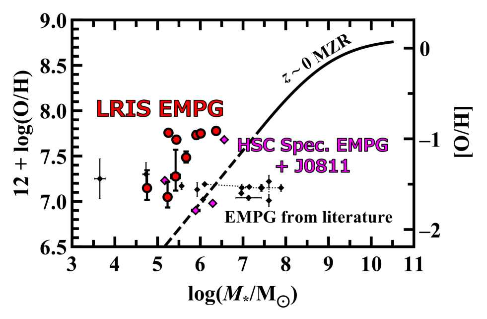
Figure 5: Mass-metallicity distribution of EMPGs. The red circles indicate the LRIS EMPGs (Section 5.1). We note that a typical uncertainty of $M_{*}$ of the LRIS EMPGs is $\sim 0.1$ dex (Section 4.3). The magenta and black diamonds show the EMPGs listed in the upper and lower parts of Table 7, respectively. The black dotted lines connecting some of the black diamonds describe that these black diamonds represent individual clumps belonging to the same EMPGs. The black solid curve is the $z\sim 0$ mass-metallicity relation (MZR) from the SDSS using the same direct-$T_{\rm e}$ method (Andrews & Martini, 2013). The black dashed line represents an extrapolation of the $z\sim 0$ MZR toward lower $M_{*}$.

Table 7: EMPGs from the literature

Name	$12+\log(\rm O/H)$	$\log(M_{*}/{\rm M}_{\odot})$	Reference
(1)	(2)	(3)	(4)
J1631+4426	$6.90\pm 0.03$	$5.89^{+0.10}_{-0.09}$	Paper I
J2314+0154	$7.23^{+0.03}_{-0.02}$	$5.17\pm 0.01$	Paper I
J2115$-$1734	$7.68\pm 0.01$	$6.56\pm 0.02$	Paper I
J0811+4730	$6.98\pm 0.02$	$6.29\pm 0.06$	Izotov et al. (2018)
AGC198691	$7.02\pm 0.03$	6.06	Hirschauer et al. (2016)
J1234+3901	$7.04\pm 0.03$	$7.13\pm 0.3$	Izotov et al. (2019)
J2229+2725	$7.09\pm 0.03$	6.96	Izotov et al. (2021)
LittleCub	$7.13\pm 0.08$	5.93	Hsyu et al. (2017)
LeoP	$7.17\pm 0.04$	5.56	Skillman et al. (2013)
J1005+3722	$7.25\pm 0.22$	$3.65\pm 0.13$	Senchyna & Stark (2019)
J0845+0131	$7.30\pm 0.13$	$4.73\pm 0.08$	Senchyna & Stark (2019)
SBS0335#1	$7.01\pm 0.07$	(7.61)	Izotov et al. (2009)
SBS0335#2	$7.22\pm 0.07$	(7.61)	Izotov et al. (2009)
DDO68#1	($7.15\pm 0.04$)	$7.44\pm 0.03$	Sacchi et al. (2016)
DDO68#2	($7.15\pm 0.04$)	$7.89\pm 0.01$	Sacchi et al. (2016)
DDO68#3	($7.15\pm 0.04$)	$7.42\pm 0.02$	Sacchi et al. (2016)
DDO68#4	($7.15\pm 0.04$)	$6.97\pm 0.03$	Sacchi et al. (2016)
IZw18NW	$7.16\pm 0.01$	7.14	Izotov & Thuan (1998)
IZw18SE	$7.19\pm 0.02$	6.10	Izotov & Thuan (1998)

As listed in Table 5, 5 out of the 10 LRIS EMPG candidates (#1, 2, 8, 9, and 10) have low metallicities of $12+\log(\rm O/H)={\color[rgb]{0,0,0}7.05}$–7.68, which meet the EMPG criterion of $12+\log(\rm O/H)\leq 7.69$. We also conclude that 4 out of the other 5 LRIS EMPG candidate (#3, 5, 6, and 7) show a low metallicity of $12+\log(\rm O/H)=7.73$–7.78 (i.e., 11–12% (O/H)_⊙). We thus refer the 9 ($=5+4$) LRIS EMPG candidates with $\lesssim 10$% (O/H)_⊙ as LRIS EMPGs. It should be noted that the other LRIS EMPG candidate (#4) still shows a low metallicity of $12+\log(\rm O/H)=7.96$ (i.e., 19% (O/H)_⊙). We emphasize that 2 out of the LRIS EMPGs (#8 and 10) show extremely-low metallicities of $12+\log(\rm O/H)={\color[rgb]{0,0,0}6.93}$–7.35 (i.e., 1.7–4.6% (O/H)_⊙) including the 1$\sigma$ uncertainties. The 2 LRIS EMPGs are thus the most metal-poor galaxies ever reported.

Figure 5 illustrates mass-metallicity distributions of the LRIS EMPGs, the HSC spectroscopic EMPGs (see Section 2), and all the other EMPGs with $12+\log(\rm O/H)<7.3$ (i.e., $<4$% (O/H)_⊙) determined by the direct-$T_{\rm e}$ method taken from the literature. The EMPGs from the literature are listed in Table 7. The mass-metallicity relation (MZR) of typical SFGs at $z\sim 0$ is well investigated and explained by the equilibrium of gas inflow/outflow and metal production by stars (e.g., Lilly et al., 2013). However, we confirm that EMPGs show a wide range of $M_{*}$ from $10^{4}$ to $10^{8}$ M_⊙, which implies that the equilibrium is not maintained at the low-mass (low-metallicity) end of the mass-metallicity distribution. Some EMPGs including many of the LRIS EMPGs lie above the extrapolation of the $z\sim 0$ MZR. Such EMPGs may be dominated by internal metal productions or outflows (Paper I), and be in the stage of the transition from gas-rich dwarf irregulars to gas-poor dwarf spheroidals (Zahid et al., 2012). As part of the on-going mid-high resolution spectroscopy survey with Magellan/MagE (EMPRESS-HRS; PI: M. Rauch), a following EMPRESS paper (Xu et al. in prep.) will report that EMPGs lying above the $z\sim 0$ MZR have broad components of emission lines with velocity widths of $\sim 200$ km s^-1, which may be attributed to the outflow. On the other hand, some of the EMPGs from the literature lie below the extrapolation of the $z\sim 0$ MZR. In such EMPGs, the contribution of metal-poor gas inflow may overwhelm the contribution of internal metal productions as discussed in Hughes et al. (2013).

We also find that LRIS EMPGs #8 and 10 also show extremely-low stellar masses of $5\times 10^{4}$–$7\times 10^{5}$ M_⊙. LRIS EMPGs #8 and 10 are helpful to understand the nature of galaxies in the very early formation phase because there have been only $\sim 7$ EMPGs reported so far to have both $12+\log(\rm O/H)\lesssim 7.3$ and $M_{*}\lesssim 10^{6}$ M_⊙. We need to explore EMPGs continuously not only to identify lowest-metallicity galaxies but also to verify whether there is a metallicity lower limit (a.k.a. metallicity floor; Prochaska et al. 2003) that local galaxies can take. Our spectroscopic observations for the EMPRESS sample continue to address the question. A recent follow-up identifies new EMPRESS EMPGs that have a stellar mass as low as $M_{*}\sim 10^{4.7}$ M_⊙ (Nakajima et al. in prep.). However, their metallicities do not fall below the currently-known metallicity floor of $\sim 1$% of the solar metallicity (e.g., Thuan et al., 2005), supporting a deficit of galaxies with metallicities below $\sim 1$% in the local universe.

5.2 Element Abundance Ratio

Table 8: EMPGs with Fe/O measurements

Name	$12+\log(\rm O/H)$	$\log(\rm Fe/O)$	$\log(\rm N/O)$	EW0(H$\beta$)	Reference
				Å
(1)	(2)	(3)	(4)	(5)	(6)
LRIS EMPG #2	$7.68^{+0.04}_{-0.03}$	$-1.74^{+0.17}_{-0.28-0.22}$	$-1.47^{+0.03}_{-0.03}$	$127^{+83}_{-33}$	This paper
LRIS EMPG #7	$7.75\pm 0.04$	$-1.66^{+0.15}_{-0.22-0.20}$	$-1.47^{+0.02}_{-0.03}$	$83^{+44}_{-11}$	This paper
J1631+4426	$6.90\pm 0.03$	$-1.25^{+0.17}_{-0.31-0.22}$	$<-1.71$	$123.5^{+3.5}_{-2.8}$	Papers I and II
J2115$-$1734	$7.68\pm 0.01$	$-1.64^{+0.03}_{-0.03-0.21}$	$-1.518^{+0.009}_{-0.011}$	$214.0^{+0.9}_{-0.8}$	Papers I and II
J0811+4730	$6.98\pm 0.02$	$-1.06^{+0.09}_{-0.09-0.22}$	$-1.535\pm 0.044$	$282.0\pm 1.0$	Izotov et al. (2018)

Figure 6 shows element abundance ratios of Ne/O, Ar/O, N/O, and Fe/O of the LRIS EMPGs and local metal-poor galaxies of Izotov et al. (2006) (gray) as functions of metallicity. As shown in the top 2 panels, the LRIS EMPGs show $\alpha$-element ratios of Ne/O and Ar/O comparable to the solar abundance ratios as well as other metal-poor galaxies.

The bottom left panel of Figure 6 presents the relations between N/O and $12+\log(\rm O/H)$, illustrating that local metal-poor galaxies present a plateau at $\log(\rm N/O)\sim-1.6$ in the range of $12+\log(\rm O/H)\lesssim 8.0$ and a positive slope at $12+\log(\rm O/H)\gtrsim 8.0$. Various studies such as Vincenzo et al. (2016; hereafter V16) suggest that the plateau and the positive slope are attributed to the primary and the secondary nucleosyntheses in massive and low-mass stars, respectively. We find that some of the LRIS EMPGs lie on the plateau. Such EMPGs are not likely to be affected by the chemical enrichment of low-mass stars but rather massive stars. We also find that LRIS EMPGs #3 and 6 lie below the plateau, showing very low N/O ratios of $\log(\rm N/O)=({\color[rgb]{0,0,0}-1.7})$–$({\color[rgb]{0,0,0}-1.8})$. The 2 LRIS EMPGs may produce oxygen selectively rather than nitrogen due to top-heavy IMFs efficiently producing massive CCSNe or high star-formation efficiencies (SFEs; defined as SFR normalized by gas mass) as discussed in Kumari et al. (2018).

The bottom right panel of Figure 6 shows the relations between Fe/O and $12+\log(\rm O/H)$. For the present case, we derive Fe/O for 2 out of the 9 LRIS EMPGs (#2 and 7) from the [Fe iii]$\lambda$4658 line detection (Section 4.1). We find that LRIS EMPGs #2 and 7 have $\log(\rm Fe/O)\sim{\color[rgb]{0,0,0}-1.7}$ and ${\rm O/H}\sim 10$% (O/H)_⊙. Adding the 2 LRIS EMPGs to 3 EMPGs with Fe/O measurements (J1631+4426, J2115$-$1734, and J0811+4730) from the literature (Paper II; Izotov et al. 2018) represented by the magenta diamonds in the bottom right panel of Figure 6, we now obtain a sample of 5 EMPGs with Fe/O measurements. We summarize properties of the 5 EMPGs in Table 8. Even considering the offsets originated from the ICF difference between Izotov et al. (2006) and Rodriguez & Rubin (2005), we confirm that J1631+4426 and J0811+4730 having the lowest O/H ratios of $\sim 2$% (O/H)_⊙ show (Fe/O)_⊙, which are higher than those of the other 3 EMPGs with $\sim 10$% (O/H)_⊙.

Based on the observations of quasar absorption systems, Becker et al. (2012) report that Fe/O ratios of the inter-galactic medium (IGM) at $z\sim 2$–6 are almost constant at a value of $[\rm Fe/O]\sim-0.4$ (i.e., $\log(\rm Fe/O)\sim-1.6$). If the $z\sim 0$ IGM also has a Fe/O value of $[\rm Fe/O]\sim-0.4$, we need some events such as SN explosions that enhance Fe/O ratios by $\gtrsim 0.4$ dex to explain high Fe/O ratios of J1631+4426 and J0811+4730. As discussed in Paper II, however, Type Ia SNe are less likely to be main contributors to enhance Fe/O ratios of J1631+4426 and J0811+4730 because of their low O/H and N/O ratios. We discuss the origin of the Fe/O enhancements quantitatively in Section 6.

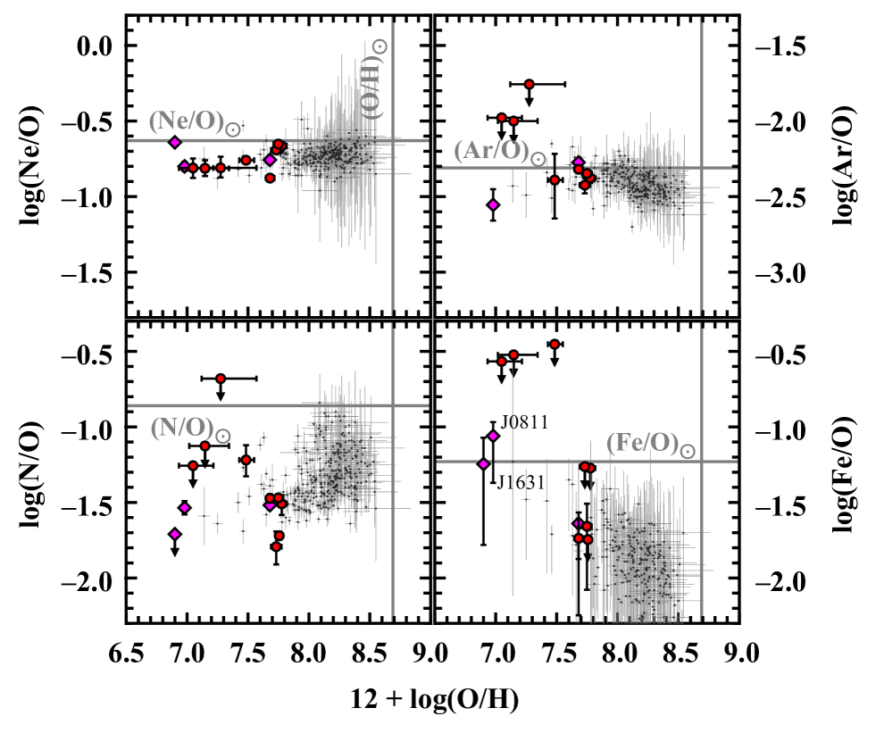
Figure 6: Gas-phase element abundance ratios of Ne/O (top left), Ar/O (top right), N/O (bottom left), and Fe/O (bottom right) as functions of $12+\log(\rm O/H)$. The symbols are the same as in Figure 5. We also add local metal-poor galaxies (Izotov et al., 2006) with the gray dots. We add 0.2-dex uncertainties to lower errors of Fe/O ratios of the local metal-poor galaxies because the Fe/O ratios are calculated from the ICF of Izotov et al. (2006; see Section 4.2). The gray solid lines represent the solar abundances (Asplund et al., 2021).

6 Origin of Fe/O Enhancements

In this section, we revisit the origin of the high Fe/O ratio of J1631+4426 and J0811+4730 with $\sim 2$% (O/H)_⊙, investigating possible contributors of HNe and PISNe that have not been discussed in Paper II (Section 1). We also re-explore the contribution of metal-poor gas inflow into EMPGs because such inflows probably trigger star-forming activities, whose effect has not evaluated in Paper II.

6.1 Considerable SN

We quantitatively explore the origin of the high Fe/O abundance ratios with Fe/O evolution models including various supernova yields. Before explaining the models, we introduce considerable SNe that would be responsible for Fe/O ratios of EMPGs.

Very massive stars with $\sim 140$–300 M_⊙ are expected to undergo thermonuclear explosions as known as PISNe (Heger & Woosley, 2002). Such a massive star above $\sim 140$ M_⊙ requires extremely metal-poor environments to form due to the efficient wind mass loss (e.g., Langer et al., 2007; Hirano et al., 2014). Especially, cores of stars with $\sim 200$–300 M_⊙ are mostly transformed into ⁵⁶Ni during the explosion (Takahashi et al., 2018). The ⁵⁶Ni atoms consequently decay to ⁵⁶Fe (Nadyozhin, 1994), which largely contribute to the Fe/O enrichment. PISNe appear $\sim 2$ Myr after the star formation, which corresponds to a lifetime of stars with $\sim 300$ M_⊙ (Takahashi et al., 2018).

Massive stars with $\sim 8$–100 M_⊙ evolve into neutron stars or black holes (BHs), undergoing CCSNe. Typical CCSNe are expected to produce low Fe/O gas because $\alpha$ elements, including oxygen, are selectively created in the massive stars during the $\alpha$ reaction (e.g., Nomoto et al., 2006). The CCSNe emerge $\sim 3$ Myr after the star formation, which corresponds to a lifetime of stars with 100 M_⊙ (Portinari et al., 1998).

Some massive stars with $\sim 30$–100 M_⊙ undergo CCSNe with explosion energies of $\gtrsim 10^{52}$ erg, which is $\sim 1$ dex larger than that of a typical CCSN of $\sim 10^{51}$ erg. Such CCSNe with high explosion energies are referred to as HNe (e.g., Iwamoto et al., 1998). The light curve model for the observed HN SN 1998bw associated with GRB 980425 shows that the mass of Fe (mostly a decay product of radioactive ⁵⁶Ni) is $\sim 0.4$ M_⊙ (Nakamura et al., 2001). This HN model with $\sim 3\times 10^{52}$ ergs for SN 1998bw yields $[\rm Fe/O]\sim-0.5$. By taking into account these observation and model of SN 1998bw, Nomoto et al. (2006, 2013) have provided yield tables giving $[\rm Fe/O]\sim-0.5$ from HNe. However, the amount of Fe in HN models depends on the explosion energy, the progenitor mass, and the mass cut that divides the ejecta and the compact remnant. Umeda & Nomoto (2008) predict that HNe with high explosion energies tend to produce higher Fe/O gas even above the solar abundance because their high temperatures promote the nucleosynthesis of ⁵⁶Ni that is decaying into ⁵⁶Fe. In addition, when we set a low value of the mass cut, HNe with normal explosion energies of $\sim 1$–$3\times 10^{52}$ erg s^-1 can also eject high Fe/O gas above the solar abundance (Umeda & Nomoto, 2008). Because HNe that eject large amount of (radioactive) ⁵⁶Ni should be bright, we refer to the HNe with high explosion energies and/or low mass cuts as bright HNe (BrHNe), hereafter. Shivvers et al. (2017) report that $\sim 1$% of observed CCSNe are HNe. However, Modjaz et al. (2020) report that galaxies hosting HNe tend to be metal-poor, which implies that HNe are preferentially born in metal-poor environments.

Low- and intermediate-mass stars evolve into white dwarfs. If a white dwarf belongs to a binary system, the system may host a Type Ia SN. A delay time of Type Ia SNe, $\tau_{\rm Ia}$, is defined to be a time from the beginning of the star formation to an appearance of the first Type Ia SN. We assume that the minimum possible $\tau_{\rm Ia}$ is 50 Myr (e.g., Mannucci et al., 2005; Sullivan et al., 2006), which is linked to the maximum zero-age main-sequence mass of stars that evolve into white dwarfs ($\sim 8$ M_⊙). Type Ia SNe can eject high Fe/O gas above the solar abundance because carbon deflagrations in white dwarfs synthesize ⁵⁶Fe.

6.2 Fe/O evolution model

Table 9: Fe/O evolution models

Model name	Mass range	Progenitor star with			Yield of
	M⊙	9–30 M⊙	30–100 M⊙	140–300 M⊙	(Br)HN or PISN
(1)	(2)	(3)	(4)	(5)	(6)
No HN/PISN	9–100	CCSN	CCSN	—	—
HN 100%	9–100	CCSN	HN	—	Nomoto et al. (2013)
BrHN 20%	9–100	CCSN	BrHN: 20% CCSN: 80%	—	Umeda & Nomoto (2008)
PISN	9–300	CCSN	CCSN	PISN	Takahashi et al. (2018)

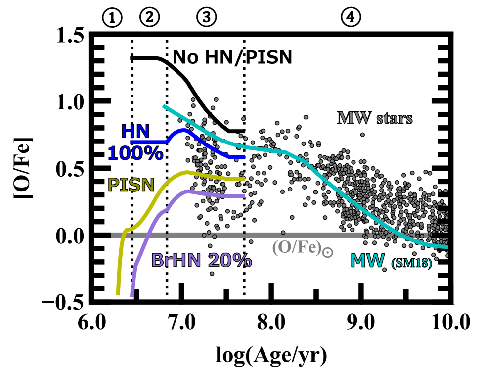
Figure 7: O/Fe evolution models. The cyan, black, blue, purple, and yellow curves indicate the MW, the No HN/PISN, the HN 100%, the BrHN 20%, and the PISN models, respectively. In Table 9, we summarize the assumptions of the models mentioned above. The gray dots show the MW stars (Edvardsson et al., 1993; Reddy et al., 2003; Gratton et al., 2003; Cayrel et al., 2004; Bensby et al., 2014; Roederer et al., 2014). The gray horizontal line indicates the solar abundance of O/Fe. From the left to the right, the vertical dotted lines show lifetimes of stars with 100, 30, and 8 M_⊙, respectively. The regions \scriptsize1⃝, \scriptsize2⃝, \scriptsize3⃝, and \scriptsize4⃝ correspond to eras in which only PISNe, CCSNe/(Br)HNe, CCSNe, and Type Ia SNe occur under the assumption of the instantaneous star-formation history, respectively.

To evaluate the contribution of Type Ia SNe, we use an Fe/O evolution model of Suzuki & Maeda (2018; hereafter SM18). We refer to this model as Milky Way (MW) model because the model is calibrated by observations of absorptions of the MW stars (e.g., Bensby et al., 2014). In the MW model, an Fe/O ratio at each age is defined as a ratio of total numbers of iron and oxygen atoms produced by all SNe that have already exploded before the age. First, SM18 create stars based on an initial mass function (IMF) of Kroupa (2001), which have mass slopes of $-2.3$, $-1.3$, and $-0.3$ for stars with $M\geq 0.5$, $0.08<M<0.5$, and $M\leq 0.08$ M_⊙, respectively. SM18 derive lifetimes of the stars as a function of star masses from Padovani & Matteucci (1993). SM18 assume that all stars below 8 M_⊙ and with 9–100 M_⊙ evolve into white dwarfs and CCSNe, respecitively, after finishing their lifetimes. The white dwarfs become Type Ia SNe following a delay-time distribution $D(t_{\rm d})$, which is proportional to $t_{\rm d}^{-1}$ and normalized so that the MW model reproduces ${\rm Fe/O}=(\rm Fe/O)_{\odot}$ at the age of the formation of the Sun. SM18 use ejecta masses (1.38 M_⊙) and element yields of Type Ia SNe predicted by Nomoto et al. (1984). SM18 also adopt a metallicity-dependent CCSN yield of Limongi & Chieffi (2006) and the best-fit star-formation history of the MW, whose SFR continuously increases until the age of $\sim 800$ Myr, and decreases to the current SFR of the MW at the age of 13.8 Gyr.

Because the MW model does not take into account ejecta from HNe or PISNe, we construct new Fe/O evolution models incorporating HNe or PISNe. Again, it is important to evaluate contributions of HNe and PISNe to the Fe/O enhancements of young metal-poor galaxies because both occur much earlier than Type Ia SNe, and also because they are preferentially born in the metal-poor environment (Modjaz et al. 2020; Langer et al. 2007). We develop models whose assumptions are summarized in Table 9. The percentages appeared in the model names represent how much fraction of stars with 30–100 M_⊙ is assumed to undergo HNe (or BrHNe). To examine whether HNe or PISNe can contribute to the Fe/O enhancements of EMPGs, we calculate Fe/O until the age of 50 Myr (i.e., before the first Type Ia SN appears). Other than this point, we construct the models in the same way as SM18. We use an IMF with a mass slope of $-2.3$ (a.k.a. Salpeter IMF; Salpeter 1955), which is common in local star-forming galaxies. Massive stars finish their lifetimes as main-sequence stars earlier than less-massive stars. We derive lifetimes of the stars as a function of star masses from the combination of Portinari et al. (1998; for 6–120 M_⊙ stars) and Takahashi et al. (2018; for 100–300 M_⊙ stars). We calculate element ejections from CCSNe, HNe, and PISNe using the most metal-poor SN yields of Nomoto et al. (2006), Nomoto et al. (2013), and Takahashi et al. (2018), respectively. Because Nomoto et al. (2006) and Nomoto et al. (2013) calculate yields of CCSNe and HNe with progenitor masses of 30 and 40 M_⊙, we extrapolate the yields to CCSNe/HNe with progenitor masses of 100 M_⊙ To create BrHNe ejecting gas with the highest Fe/O, we use yields of Umeda & Nomoto (2008) with the highest explosion energy and the lowest mass cut just above the Fe core at a given progenitor star mass. For all the models, we assume that 1) all stars with 9–30 M_⊙ explode as CCSNe, 2) all stars with 100–140 M_⊙ undergo direct collapses that eject no element, and 3) the star formation occurs at once at the beginning of the galaxy formation (i.e., instantaneous star-formation history).

Figure 7 illustrates the Fe/O evolution models, while we convert Fe/O to O/Fe normalized by the solar abundance ([O/Fe]). We find that the BrHN 20% (purple) and PISN (yellow) models show low O/Fe (high Fe/O) ratios comparable to the solar abundance during the \scriptsize1⃝ and \scriptsize2⃝ eras. The HN 100% (blue), BrHN 20%, and PISN models show maximum O/Fe (minimum Fe/O) values at $\sim$10 Myr mainly because the high-Fe/O gas produced by HNe or PISNe is diluted with the low-Fe/O gas efficiently ejected from CCSNe whose progenitor masses are $\gtrsim 20$ M_⊙. The MW model (cyan) predicts that the O/Fe (Fe/O) value continuously decrease (increase) with the age. The decrease in O/Fe (increase in Fe/O) during the \scriptsize4⃝ era is mainly attributed to Type Ia SNe.

The gray dots in Figure 7 show the distribution of the MW stars (Edvardsson et al., 1993; Reddy et al., 2003; Gratton et al., 2003; Cayrel et al., 2004; Bensby et al., 2014; Roederer et al., 2014). Because we cannot determine [Fe/H] evolutions of the (Br)HN/PISN models due to uncertainties of evolution models of gas masses (and thus hydrogen abundances) of EMPGs, we convert [Fe/H] of the MW stars to the age using the [Fe/H] evolution models of SM18 instead. The MW model reproduces the distribution of the MW stars especially during the \scriptsize4⃝ era (i.e., $[\rm Fe/H]\gtrsim-2$), which indicates that the contribution of Type Ia SNe is properly incorporated into the MW model. In the \scriptsize3⃝ era (i.e., $[\rm Fe/H]\lesssim-2$), however, the MW model cannot explain the distribution of the MW stars with low O/Fe (high Fe/O) ratios. The BrHN and the PISN models reproduce the distribution of the MW stars with low O/Fe ratios of $[\rm O/Fe]=0.3$–0.4, which implies that some metal-poor stars contain elements from HNe or PISNe as discussed in Aoki et al. (2014). We may need HNe or PISNe other than Type Ia SNe or CCSNe to reproduce the chemical enrichment of galaxies in the early formation phase.

Finally, we convert the model age to EW₀(H$\beta$) because the stellar age used in the models is not an observable. Using the beagle code calculating both the stellar continuum and the nebular emission (cf. Section 4.3), Paper I derives EW₀(H$\alpha$) as a function of stellar age and $12+\log(\rm O/H)$ under the assumption of the constant star formation. Basically, EW₀(H$\alpha$) increases as $12+\log(\rm O/H)$ decreases because metal-poor stars make stellar continua harder (e.g., Tumlinson & Shull, 2000). To remove the $12+\log(\rm O/H)$ dependency, we assume a relation between O/H and stellar age of the Milky Way model (SM18). Using an empirical relation of ${\rm EW}_{0}({\rm H}\alpha)=5.47\times{\rm EW}_{0}({\rm H}\beta)$ (Paper I), we obtain a relation between EW₀(H$\beta$) and the stellar age.

Here we evaluate the uncertainty in the conversion from the stellar age to EW₀(H$\beta$). Paper I and Izotov et al. (2018) report that J1631+4426 and J0811+4730 have stellar ages of 50 and 3.3 Myr and EW₀(H$\beta$) of 120 and 280 Å, respectively. Using the relation between EW₀(H$\beta$) and the stellar age, we find that the stellar ages of 50 and 3.3 Myr correspond to EW₀(H$\beta$) of 90 and 380 Å, respectively. The stellar ages inferred from EW₀(H$\beta$) are different from those from the literature by $\sim 0.13$ dex. Thus, we add the $\pm 0.13$-dex uncertainties to EW₀(H$\beta$) values of the Fe/O evolution models.

Although the models provide total ($={\rm gas}+{\rm dust}+{\rm stellar}$) Fe/O ratios, we note that the gas-phase Fe/O ratios of dust-poor and low-$M_{*}$ EMPGs are expected to be comparable to the total Fe/O ratios (and thus the Fe/O ratios predicted by the models) because we can ignore the amount of ejecta of SNe trapped in dust grains and stars.

6.3 Possible scenario

To explain the Fe/O enhancements, we investigate 3 scenarios of 1) Type Ia SN, 2) gas dilution and episodic star formation, and 3) HN, BrHN, or PISN.

6.3.1 Type Ia SN

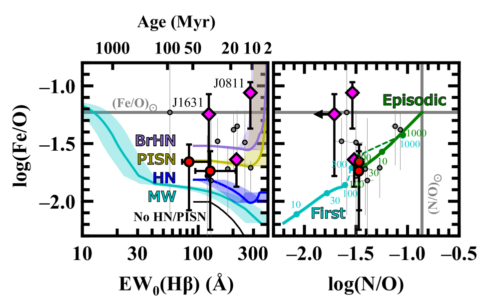
Figure 8: Fe/O ratio as a function of ${\rm EW}_{0}({\rm H}\beta)$ and N/O described in the left and right panels, respectively. The gray circles indicate local metal-poor galaxies (Izotov et al., 2006), which are the same as in Figure 6 but limited to those with $12+\log(\rm O/H)\leq 7.69$. Regarding the local metal-poor galaxies (Izotov et al., 2006), we only show errors of Fe/O. The other symbols are the same as in Figure 6, but limited to those with Fe/O measurements or strong upper limits of Fe/O. In the left panel, the cyan, blue, purple, and yellow curves with the shaded regions show the MW, the HN 100%, the BrHN 20%, and the PISN models, respectively. The black curve indicates the No HN/PISN model. In the right panel, the cyan and green curves represent evolution tracks of Fe/O and N/O when first and episodic starbursts occur in a galaxy, respectively. The numbers accompanied by the curves indicate the ages in the unit of Myr. We draw the evolution tracks with solid and dashed lines before and after 100 Myr, respectively, because all the EMPGs shown in the left panel have ages $\lesssim 100$ Myr. To predict Fe/O and N/O ratios, we use the MW model (SM18) and the V16 model, respectively. The gray lines show the solar abundances (Asplund et al., 2021).

First, we quantitatively check whether Type Ia SNe are not responsible for the Fe/O enhancements as concluded by Paper II. Below, we use the MW model (SM18), in which only Type Ia SNe can eject iron-rich gas. In the left panel of Figure 8, we show the MW model represented by the cyan curve with the shaded region, respectively. The Fe/O value increases as the EW₀(H$\beta$) value decreases (and thus the age increases) especially in the range of EW₀(H$\beta)\lesssim 50$ Å (i.e., $\gtrsim 100$ Myr) because of the appearance of Type Ia SNe.

We find that J0811+4730 shows the Fe/O value significantly higher than the MW model prediction with a little uncertainty. J0811+4730 has a large EW₀(H$\beta$) of $\sim 300$ Å corresponding to an extremely-young age of $\sim 10$ Myr, which suggests that Type Ia SNe, whose minimum possible delay time is 50 Myr (Section 6.1), cannot contribute to the Fe/O enhancement of J0811+4730. Thus, we can rule out the first scenario for J0811+4730. We can also reject the possibility that the Fe/O value of J1631+4426 is consistent with the MW model with at least $\sim 1\sigma$ level. In addition, the Fe/O excess of J1631+4426 from the MW model may become larger because J1631+4426 has an EMPG-tail (Paper III; see Section 3.1), which potentially makes the EW of J1631+4426 underestimated by a factor of 2 (Section 4.1). We thus conclude that the Fe/O enhancement of J1631+4426 is not likely to be attributed to Type Ia SNe.

Relations between Fe/O and N/O of J1631+4426 and J0811+4730 also support the conclusion mentioned above. To estimate the N/O enrichment, we utilize a chemical evolution model of V16. Because V16 implement the primary nucleosynthesis of nitrogen in massive stars (Romano et al., 2010), the V16 model can reproduce the observed relation between N/O and $12+\log(\rm O/H)$ of local star-forming galaxies within a wide metallicity range of $12+\log(\rm O/H)\sim 7.2$–8.7. In the right panel of Figure 8, we show evolution tracks of the relation between Fe/O and N/O based on the MW model (SM18) and the V16 model represented by the cyan solid curve. We find that J0811+4730 and J1631+4426 have very high Fe/O and low N/O ratios, which cannot be reproduced by the first star-formation model. We conclude again that Type Ia SNe are not likely to enhance the Fe/O ratios of J0811+4730 and J1631+4426.

We note that the EMPGs other than J0811+4730 or J1631+4426 also have young ages of $<100$ Myr inferred from their large EW₀(H$\beta$) as shown in the left panel of Figure 8. However, none of the EMPGs are consistent with the first star-formation model with ages less than 100 Myr as illustrated in the right panel of Figure 8. This indicates that Type Ia SNe are not responsible for Fe/O ratios of typical EMPGs.

6.3.2 Gas dilution and episodic star formation

The second scenario is a combination of gas dilution and episodic star formation caused by primordial gas inflow. Paper III reports that more than 80% of EMPGs have EMPG-tails. Sánchez Almeida et al. (2015) report that EMPG-tails have O/H ratios $\sim 1$ dex larger than those of EMPGs, which suggests that metal-poor gas accretions onto EMPG-tails trigger star-formation activities of EMPGs. If EMPGs and EMPG-tails originally share the same gas, it is possible that the EMPGs have high Fe/O gas produced by past star formations in the EMPG-tails.

In this section, we assume that EMPGs originally have all element abundances equal to the solar abundances based on the fact that a typical EMPG-tail has ${\rm O/H}\sim(\rm O/H)_{\odot}$ (Sánchez Almeida et al., 2015). Then, we investigate how element abundance ratios of the EMPGs change after the metal-poor gas inflow into the EMPGs. If the $z\sim 0$ IGM also has an Fe/O ratio of $[\rm Fe/O]\sim-0.4$ comparable to those at $z\gtrsim 2$ (Becker et al., 2012), an IGM-gas inflow onto an EMPG may decrease Fe/O of the EMPG. However, the decline is probably negligible because the IGM metallicity in the local universe may have a lower limit of $\sim 10^{-2}$ Z_⊙ (e.g., Thuan et al., 2005). For the sake of simplicity, we assume primordial (i.e., only hydrogen) gas inflow. Just after the original gas components of the EMPGs are diluted with the primordial gas, metal-to-hydrogen ratios such as $12+\log(\rm O/H)$ decreases while Fe/O ratios remain comparable to (Fe/O)_⊙. However, N/O ratios should also be similar to (N/O)_⊙, whereas the EMPGs have N/O ratios significantly lower than (N/O)_⊙ as described in the left bottom panel of Figure 6. Thus, the dilution of the solar-metallicity gas with the primordial gas cannot explain the Fe/O enhancements of the EMPGs by itself as discussed in Paper II.

However, the primordial gas inflow can trigger the episodic star formation, which potentially impacts element abundance ratios of the whole EMPG due to its low stellar mass. Especially, the N/O ratio is expected to decrease until $\sim 100$ Myr after the episodic star formation because massive stars produce low N/O gas of $\sim 20$% (N/O)_⊙ (V16). Thus, we investigate the contribution of the episodic star formation, which has not been investigated in Paper II. As in Section 6.3.1, we adopt the MW model and the V16 model to predict Fe/O and N/O evolutions, respectively. Assuming that the inflow quintuples the gas mass of the galaxy after finishing the first major star formation, we calculate the evolution track of the episodic starburst as shown in the right panel of Figure 8 with the green solid curve.

Regarding J1631+4426 and J0811+4730, we identify that even the episodic star-formation model cannot reproduce the high Fe/O, the low N/O, and the young ages of $\lesssim 50$ Myr at the same time. Of course, we can create episodic star-formation models that satisfy the high Fe/O, the low N/O, and the young ages of the EMPGs by arbitrarily assuming that the EMPGs originally have high Fe/O and low N/O ratios. However, such an assumption is unlikely to be plausible because the first burst model at any age does not reproduce high Fe/O and low N/O ratios simultaneously. We conclude that the second scenario can be ruled out for J1631+4426 and J0811+4730 even if the inflow triggers the episodic starburst.

We note that many of the EMPGs other than J1631+4426 or J0811+4730 have relatively high Fe/O and N/O ratios comparable to those predicted by the episodic star-formation model within the range of $<100$ Myr. These EMPGs may have old gas populations that are already affected by Type Ia SNe and AGB stars as discussed in Sánchez Almeida et al. (2016).

6.3.3 HN, BrHN, or PISN

The third scenario is the contribution of HNe, BrHNe, or PISNe, which has not been investigated in Paper II. The left panel of Figure 8 illustrates the models containing HNe, BrHNe, or PISNe (Table 9). We find that either the BrHN 20% (purple) or the PISN (yellow) models can reproduce the relations between Fe/O and EW${}_{0}({\rm H}\beta)$ of J1631+4426 and J0811+4730. We also find that we cannot explain the Fe/O enhancements even with the HN 100% model (blue), which implies that HNe with relatively-low explosion energies of $\sim 10^{52}$ erg and reasonable mass cuts are not responsible for the Fe/O enhancements. We conclude that BrHNe or PISNe can contribute to the Fe/O enhancements of J1631+4426 and J0811+4730. The N/O ratio potentially isolate BrHNe from PISNe. We need BrHN and PISN yields that plausibly calculate the primary nucleosynthesis of nitrogen as implemented in V16.

We note that most of the EMPGs in Figure 8 are also in agreement with either the BrHN 20% or the PISN models. This may trace the (past) presence of BrHNe or PISNe in the EMPGs (with moderate Fe/O ratios). Some of the EMPGs have low Fe/O ratios comparable to that predicted by the HN 100% model. Such EMPGs may be affected by (normal) HNe.

One may wonder whether the presence of BrHNe or PISNe conflicts with the positive trend between O/Fe and Fe/H ratios of the MW stars (as well as stars in satellite galaxies of the MW; e.g., Pompéia et al. 2008), which is an observational support of a cosmic clock. However, the positive trend is clear only within the range of $[\rm Fe/H]\gtrsim-2$, which corresponds to the formation age of the MW of $\gtrsim 50$ Myr in Figure 7. Stars below $[\rm Fe/H]\lesssim-2$ (the formation age of the MW less than $\sim 50$ Myr) show a wide range of [O/Fe] from $\sim-0.3$ to 1.0, which allows the presence of BrHNe or PISNe (see Section 6.2).

6.3.4 Conclusion

We have investigated the 3 scenarios that can explain the Fe/O enhancements of J1631+4426 and J0811+4730 with $\sim 2$% (O/H)_⊙ and low N/O ratios. We conclude that the Fe/O enhancements are not likely to be explained by the Type Ia SN or the episodic star-formation scenarios but an inclusion of BrHNe and/or PISNe. This conclusion implies that first galaxies at $z\sim 10$ with metallicities of 0.1–1% Z_⊙ (Wise et al., 2012) could also have high Fe/O ratios because HNe and PISNe are preferentially produced in metal-poor environments (Section 6.1). Our conclusion also suggests that galaxies with high Fe/O ratios are not necessarily old enough to be affected by Type Ia SNe. This infers that Fe/O would not serve as a cosmic clock in primordial galaxies because not Type Ia SNe but HNe or PISNe are likely to be responsible for the Fe/O enhancements in young metal-poor galaxies.

We note that Fe/O ratios of the EMPGs other than J1631+4426 or J0811+4730 can be generally explained by either episodic star formation or (Br)HNe/PISNe due to their moderate Fe/O and N/O ratios compared with J1631+4426 and J0811+4730. Primordial galaxies such as J1631+4426 and J0811+4730 are thus important to verify the presence of BrHNe or PISNe.

7 Summary

We present element abundance ratios of local EMPGs, which are expected to be galaxies in the early formation phase. We conduct spectroscopic follow-up observations for 13 faint EMPG candidates selected by EMPRESS with Keck/LRIS. We newly identify 9 EMPGs with ${\rm O/H}=2.2$–12% (O/H)_⊙ at $z=0.009$–0.057. Notably, 2 out of the 9 EMPGs have extremely-low stellar masses and oxygen abundances of $5\times 10^{4}$–$7\times 10^{5}$ M_⊙ and 2–3% (O/H)_⊙, respectively, indicative that the 2 EMPGs are galaxies in the very early formation phase. Comparing nucleosynthesis models with representative EMPGs, we pinpoint J1631+4426 and J0811+4730 having the lowest O/H ratios of $\sim 2$% (O/H)_⊙, whose high Fe/O and low N/O ratios cannot be explained by Type Ia supernovae (SNe) or episodic star formation but bright hypernovae (BrHNe; Section 6.1) and/or pair-instability SNe (PISNe). Because HNe and PISNe are preferentially produced in metal-poor environments, primordial galaxies at $z\sim 10$ potentially have high Fe/O values as well as the EMPGs. We also suggest that the Fe/O ratio may not serve as a cosmic clock for primordial galaxies.

References

- Aihara et al. (2019) Aihara, H., AlSayyad, Y., Ando, M., et al. 2019, PASJ, doi: 10.1093/pasj/psz103
- Andrews & Martini (2013) Andrews, B. H., & Martini, P. 2013, ApJ, doi: 10.1088/0004-637X/765/2/140
- Aoki et al. (2014) Aoki, W., Tominaga, N., Beers, T. C., Honda, S., & Lee, Y. S. 2014, Science, 345, 912, doi: 10.1126/science.1252633
- Asplund et al. (2021) Asplund, M., Amarsi, A. M., & Grevesse, N. 2021, A&A, 653, A141, doi: 10.1051/0004-6361/202140445
- Becker et al. (2012) Becker, G. D., Sargent, W. L. W., Rauch, M., & Carswell, R. F. 2012, ApJ, 744, 91, doi: 10.1088/0004-637X/744/2/91
- Behroozi et al. (2013) Behroozi, P. S., Wechsler, R. H., & Conroy, C. 2013, ApJ, 770, doi: 10.1088/0004-637X/770/1/57
- Bèland et al. (1988) Bèland, S., Boulade, O., & Davidge, T. 1988, Bulletin d’information du telescope Canada-France-Hawaii, 19, 16
- Bensby et al. (2014) Bensby, T., Feltzing, S., & Oey, M. S. 2014, A&A, 562, A71, doi: 10.1051/0004-6361/201322631
- Berg et al. (2019) Berg, D. A., Erb, D. K., Henry, R. B. C., Skillman, E. D., & McQuinn, K. B. W. 2019, ApJ, 874, 93, doi: 10.3847/1538-4357/ab020a
- Berg et al. (2015) Berg, D. A., Skillman, E. D., Croxall, K. V., et al. 2015, ApJ, 806, 16, doi: 10.1088/0004-637X/806/1/16
- Bruzual & Charlot (2003) Bruzual, G., & Charlot, S. 2003, MNRAS, doi: 10.1046/j.1365-8711.2003.06897.x
- Calzetti et al. (2000) Calzetti, D., Armus, L., Bohlin, R. C., et al. 2000, ApJ, 533, 682, doi: 10.1086/308692
- Calzetti et al. (1994) Calzetti, D., Kinney, A. L., & Storchi-Bergmann, T. 1994, ApJ, 429, 582, doi: 10.1086/174346
- Cayrel et al. (2004) Cayrel, R., Depagne, E., Spite, M., et al. 2004, A&A, 416, 1117, doi: 10.1051/0004-6361:20034074
- Chabrier (2003) Chabrier, G. 2003, PASP, doi: 10.1086/376392
- Chevallard & Charlot (2016) Chevallard, J., & Charlot, S. 2016, MNRAS, 462, 1415, doi: 10.1093/mnras/stw1756
- Edvardsson et al. (1993) Edvardsson, B., Andersen, J., Gustafsson, B., et al. 1993, A&A, 500, 391
- Ferland et al. (2013) Ferland, G. J., Porter, R. L., Van Hoof, P. A., et al. 2013, The 2013 release of CLOUDY. https://arxiv.org/abs/1302.4485
- Froese Fischer & Tachiev (2004) Froese Fischer, C., & Tachiev, G. 2004, Atomic Data and Nuclear Data Tables, 87, 1, doi: 10.1016/j.adt.2004.02.001
- Gardner et al. (2006) Gardner, J. P., Mather, J. C., Clampin, M., et al. 2006, Space Science Reviews, 123, 485, doi: 10.1007/s11214-006-8315-7
- Garnett (1992) Garnett, D. R. 1992, AJ, doi: 10.1086/116146
- Gratton et al. (2003) Gratton, R. G., Carretta, E., Claudi, R., Lucatello, S., & Barbieri, M. 2003, A&A, 404, 187, doi: 10.1051/0004-6361:20030439
- Gutkin et al. (2016) Gutkin, J., Charlot, S., & Bruzual, G. 2016, MNRAS, doi: 10.1093/mnras/stw1716
- Hees et al. (2015) Hees, a., Hestroffer, D., Poncin-Lafitte, C. L., & David, P. 2015, Research in Astronomy and Astrophysics, 15, 1945. https://arxiv.org/abs/1509.06868
- Heger & Woosley (2002) Heger, A., & Woosley, S. E. 2002, ApJ, doi: 10.1086/338487
- Hirano et al. (2015) Hirano, S., Hosokawa, T., Yoshida, N., Omukai, K., & Yorke, H. W. 2015, MNRAS, 448, 568, doi: 10.1093/mnras/stv044
- Hirano et al. (2014) Hirano, S., Hosokawa, T., Yoshida, N., et al. 2014, ApJ, doi: 10.1088/0004-637X/781/2/60
- Hirschauer et al. (2016) Hirschauer, A. S., Salzer, J. J., Skillman, E. D., et al. 2016, ApJ, doi: 10.3847/0004-637x/822/2/108
- Hsyu et al. (2017) Hsyu, T., Cooke, R. J., Prochaska, J. X., & Bolte, M. 2017, ApJ, doi: 10.3847/2041-8213/aa821f
- Hsyu et al. (2018) —. 2018, ApJ, 863, 134, doi: 10.3847/1538-4357/aad18a
- Huang et al. (2018) Huang, S., Leauthaud, A., Murata, R., et al. 2018, PASJ, 70, S6, doi: 10.1093/pasj/psx126
- Hughes et al. (2013) Hughes, T. M., Cortese, L., Boselli, A., Gavazzi, G., & Davies, J. I. 2013, A&A, 550, A115, doi: 10.1051/0004-6361/201218822
- Inoue (2011) Inoue, A. K. 2011, MNRAS, doi: 10.1111/j.1365-2966.2011.18906.x
- Isobe et al. (2021) Isobe, Y., Ouchi, M., Kojima, T., et al. 2021, ApJ in Press. https://arxiv.org/abs/2004.11444
- Iwamoto et al. (1998) Iwamoto, K., Mazzali, P. A., Nomoto, K., et al. 1998, Nature, 395, 672, doi: 10.1038/27155
- Izotov et al. (2009) Izotov, Y. I., Guseva, N. G., Fricke, K. J., & Papaderos, P. 2009, A&A, doi: 10.1051/0004-6361/200911965
- Izotov et al. (2006) Izotov, Y. I., Stasińska, G., Meynet, G., Guseva, N. G., & Thuan, T. X. 2006, A&A, 448, 955, doi: 10.1051/0004-6361:20053763
- Izotov & Thuan (1998) Izotov, Y. I., & Thuan, T. X. 1998, ApJ, 497, 227, doi: 10.1086/305440
- Izotov et al. (2019) Izotov, Y. I., Thuan, T. X., & Guseva, N. G. 2019, MNRAS, 483, 5491, doi: 10.1093/mnras/sty3472
- Izotov et al. (2021) Izotov, Y. I., Thuan, T. X., & Guseva, N. G. 2021, MNRAS, 504, 3996, doi: 10.1093/mnras/stab1099
- Izotov et al. (2018) Izotov, Y. I., Worseck, G., Schaerer, D., et al. 2018, MNRAS, 478, 4851, doi: 10.1093/mnras/sty1378
- James et al. (2015) James, B. L., Koposov, S., Stark, D. P., et al. 2015, MNRAS, 448, 2687, doi: 10.1093/mnras/stv175
- James et al. (2017) James, B. L., Koposov, S. E., Stark, D. P., et al. 2017, MNRAS, 465, 3977, doi: 10.1093/mnras/stw2962
- Johansson et al. (2000) Johansson, S., Zethson, T., Hartman, H., et al. 2000, A&A, 361, 977
- Kikuchihara et al. (2020) Kikuchihara, S., Ouchi, M., Ono, Y., et al. 2020, ApJ, doi: 10.3847/1538-4357/ab7dbe
- Kisielius et al. (2009) Kisielius, R., Storey, P. J., Ferland, G. J., & Keenan, F. P. 2009, MNRAS, 397, 903, doi: 10.1111/j.1365-2966.2009.14989.x
- Kojima et al. (2020) Kojima, T., Ouchi, M., Rauch, M., et al. 2020, ApJ, 898, 142, doi: 10.3847/1538-4357/aba047
- Kojima et al. (2021) Kojima, T., Ouchi, M., Rauch, M., et al. 2021, ApJ, 913, 22, doi: 10.3847/1538-4357/abec3d
- Kroupa (2001) Kroupa, P. 2001, MNRAS, doi: 10.1046/j.1365-8711.2001.04022.x
- Kumari et al. (2018) Kumari, N., James, B. L., Irwin, M. J., Amorín, R., & Pérez-Montero, E. 2018, MNRAS, 476, 3793, doi: 10.1093/mnras/sty402
- Langer et al. (2007) Langer, N., Norman, C. A., de Koter, A., et al. 2007, A&A, 475, L19, doi: 10.1051/0004-6361:20078482
- Lilly et al. (2013) Lilly, S. J., Carollo, C. M., Pipino, A., Renzini, A., & Peng, Y. 2013, ApJ, 772, 119, doi: 10.1088/0004-637X/772/2/119
- Limongi & Chieffi (2006) Limongi, M., & Chieffi, A. 2006, ApJ, 647, 483, doi: 10.1086/505164
- Luridiana et al. (2015) Luridiana, V., Morisset, C., & Shaw, R. A. 2015, A&A, 573, A42, doi: 10.1051/0004-6361/201323152
- Mannucci et al. (2005) Mannucci, F., Valle, M. D., & Panagia, N. 2005, arXiv
- McLaughlin & Bell (2000) McLaughlin, B. M., & Bell, K. L. 2000, JPhB, 33, 597, doi: 10.1088/0953-4075/33/4/301
- Modjaz et al. (2020) Modjaz, M., Bianco, F. B., Siwek, M., et al. 2020, ApJ, 892, 153, doi: 10.3847/1538-4357/ab4185
- Morales-Luis et al. (2011) Morales-Luis, A. B., Sánchez Almeida, J., Aguerri, J. A., & Mũoz-Tũón, C. 2011, ApJ, 743, doi: 10.1088/0004-637X/743/1/77
- Munoz Burgos et al. (2009) Munoz Burgos, J. M., Loch, S. D., Ballance, C. P., & Boivin, R. F. 2009, A&A, 500, 1253, doi: 10.1051/0004-6361/200911743
- Nadyozhin (1994) Nadyozhin, D. K. 1994, ApJS, 92, 527, doi: 10.1086/192008
- Nakamura et al. (2001) Nakamura, T., Mazzali, P. A., Nomoto, K., & Iwamoto, K. 2001, ApJ, 550, 991, doi: 10.1086/319784
- Nomoto et al. (2013) Nomoto, K., Kobayashi, C., & Tominaga, N. 2013, ARA&A, 51, 457, doi: 10.1146/annurev-astro-082812-140956
- Nomoto et al. (1984) Nomoto, K., Thielemann, F. K., & Yokoi, K. 1984, ApJ, 286, 644, doi: 10.1086/162639
- Nomoto et al. (2006) Nomoto, K., Tominaga, N., Umeda, H., Kobayashi, C., & Maeda, K. 2006, Nucl. Phys. A, 777, 424, doi: 10.1016/j.nuclphysa.2006.05.008
- Oke & Gunn (1983) Oke, J. B., & Gunn, J. E. 1983, ApJ, doi: 10.1086/160817
- Oke et al. (1995) Oke, J. B., Cohen, J. G., Carr, M., et al. 1995, PASP, 107, 375, doi: 10.1086/133562
- Ono et al. (2018) Ono, Y., Ouchi, M., Harikane, Y., et al. 2018, PASJ, doi: 10.1093/pasj/psx103
- Padovani & Matteucci (1993) Padovani, P., & Matteucci, F. 1993, ApJ, doi: 10.1086/173212
- Pompéia et al. (2008) Pompéia, L., Hill, V., Spite, M., et al. 2008, A&A, 480, 379, doi: 10.1051/0004-6361:20064854
- Portinari et al. (1998) Portinari, L., Chiosi, C., & Bressan, A. 1998, A&A, 334, 505. https://arxiv.org/abs/astro-ph/9711337
- Prochaska et al. (2003) Prochaska, J. X., Gawiser, E., Wolfe, A. M., Castro, S., & Djorgovski, S. G. 2003, ApJ, 595, L9. https://iopscience.iop.org/article/10.1086/378945
- Pustilnik et al. (2005) Pustilnik, S. A., Kniazev, A. Y., & Pramskij, A. G. 2005, A&A, doi: 10.1051/0004-6361:20053102
- Quinet (1996) Quinet, P. 1996, A&AS, 116, 573
- Reddy et al. (2003) Reddy, B. E., Tomkin, J., Lambert, D. L., & Allende Prieto, C. 2003, MNRAS, 340, 304, doi: 10.1046/j.1365-8711.2003.06305.x
- Rodriguez & Rubin (2005) Rodriguez, M., & Rubin, R. H. 2005, ApJ, doi: 10.1086/429958
- Roederer et al. (2014) Roederer, I. U., Preston, G. W., Thompson, I. B., et al. 2014, AJ, 147, 136, doi: 10.1088/0004-6256/147/6/136
- Romano et al. (2010) Romano, D., Karakas, A. I., Tosi, M., & Matteucci, F. 2010, A&A, 522, A32, doi: 10.1051/0004-6361/201014483
- Sacchi et al. (2016) Sacchi, E., Annibali, F., Cignoni, M., et al. 2016, ApJ, 830, 3, doi: 10.3847/0004-637x/830/1/3
- Salpeter (1955) Salpeter, E. E. 1955, ApJ, doi: 10.1086/145971
- Sánchez Almeida et al. (2016) Sánchez Almeida, J., Perez-Montero, E., Morales-Luis, A. B., et al. 2016, ApJ, 819, 110, doi: 10.3847/0004-637X/819/2/110
- Sánchez Almeida et al. (2015) Sánchez Almeida, J., Elmegreen, B. G., Muñoz-Tuón, C., et al. 2015, ApJL, 810, L15, doi: 10.1088/2041-8205/810/2/L15
- Schlafly & Finkbeiner (2011) Schlafly, E. F., & Finkbeiner, D. P. 2011, ApJ, 737, doi: 10.1088/0004-637X/737/2/103
- Senchyna & Stark (2019) Senchyna, P., & Stark, D. P. 2019, MNRAS, 484, 1270, doi: 10.1093/mnras/stz058
- Shibata & Shapiro (2002) Shibata, M., & Shapiro, S. L. 2002, ApJ, 572, L39, doi: 10.1086/341516
- Shivvers et al. (2017) Shivvers, I., Modjaz, M., Zheng, W., et al. 2017, PASP, 129, 54201, doi: 10.1088/1538-3873/aa54a6
- Skillman et al. (2013) Skillman, E. D., Salzer, J. J., Berg, D. A., et al. 2013, AJ, doi: 10.1088/0004-6256/146/1/3
- Storey & Hummer (1995) Storey, P. J., & Hummer, D. G. 1995, MNRAS, 272, 41, doi: 10.1093/mnras/272.1.41
- Storey et al. (2014) Storey, P. J., Sochi, T., & Badnell, N. R. 2014, MNRAS, 441, 3028, doi: 10.1093/mnras/stu777
- Sullivan et al. (2006) Sullivan, M., Le Borgne, D., Pritchet, C. J., et al. 2006, ApJ, doi: 10.1086/506137
- Suzuki & Maeda (2018) Suzuki, A., & Maeda, K. 2018, ApJ, 852, 101, doi: 10.3847/1538-4357/aaa024
- Takahashi et al. (2018) Takahashi, K., Yoshida, T., & Umeda, H. 2018, arXiv, doi: 10.3847/1538-4357/aab95f
- Tayal (2011) Tayal, S. S. 2011, ApJS, 195, 12, doi: 10.1088/0067-0049/195/2/12
- Thuan et al. (2005) Thuan, T. X., Lecavelier des Etangs, A., & Izotov, Y. I. 2005, ApJ, 621, 269, doi: 10.1086/427469
- Totani et al. (2008) Totani, T., Morokuma, T., Oda, T., Doi, M., & Yasuda, N. 2008, PASJ, 60, 1327, doi: 10.1093/pasj/60.6.1327
- Tumlinson & Shull (2000) Tumlinson, J., & Shull, J. M. 2000, ApJ, 528, L65, doi: 10.1086/312432
- Umeda & Nomoto (2008) Umeda, H., & Nomoto, K. 2008, ApJ, 673, 1014, doi: 10.1086/524767
- Vincenzo et al. (2016) Vincenzo, F., Belfiore, F., Maiolino, R., Matteucci, F., & Ventura, P. 2016, MNRAS, 458, 3466, doi: 10.1093/mnras/stw532
- Vink (2018) Vink, J. S. 2018, A&A, 615, A119, doi: 10.1051/0004-6361/201832773
- Wise et al. (2012) Wise, J. H., Turk, M. J., Norman, M. L., & Abel, T. 2012, ApJ, 745, doi: 10.1088/0004-637X/745/1/50
- Xing et al. (2019) Xing, Q.-F., Zhao, G., Aoki, W., et al. 2019, Nature Astronomy, 3, 631, doi: 10.1038/s41550-019-0764-5
- Zahid et al. (2012) Zahid, H. J., Bresolin, F., Kewley, L. J., Coil, A. L., & Davé, R. 2012, ApJ, 750, 120, doi: 10.1088/0004-637X/750/2/120
- Zhang (1996) Zhang, H. 1996, AAS, 119, 523, doi: 10.1051/aas:1996264