Bob and Alice Go to a Bar

Abstract

It is well known that reinforcement learning can be cast as inference in an appropriate probabilistic model. However, this commonly involves introducing a distribution over agent trajectories with probabilities proportional to exponentiated rewards. In this work, we formulate reinforcement learning as Bayesian inference without resorting to rewards, and show that rewards are derived from agent’s preferences, rather than the other way around. We argue that agent preferences should be specified stochastically rather than deterministically. Reinforcement learning via inference with stochastic preferences naturally describes agent behaviors, does not require introducing rewards and exponential weighing of trajectories, and allows to reason about agents using the solid foundation of Bayesian statistics. Stochastic conditioning, a probabilistic programming paradigm for conditioning models on distributions rather than values, is the formalism behind agents with probabilistic preferences. We demonstrate realization of our approach on case studies using both a two-agent coordinate game and a single agent acting in a noisy environment, showing that despite superficial differences, both cases can be modelled and reasoned about based on the same principles.

1 Introduction

The ‘planning as inference’ paradigm [WGR⁺11, vdMPTW16] extends Bayesian inference to future observations. The agent in the environment is modelled as a Bayesian generative model, but the belief about the distribution of agent’s actions is updated based on future goals rather than on past facts. This allows to use common modelling and inference tools, notably probabilistic programming, to represent computer agents and explore their behavior. Representing agents as general programs provides flexibility compared to restricted approaches, such as Markov decision processes and their variants and extensions, and allows to model a broad range of complex behaviors in a unified and natural way.

Planning, or, more generally, reinforcement learning, as inference models agent preferences through conditioning agents on preferred future behaviors. Often, the conditioning is achieved through the Boltzmann distribution: the probability of a realization of agent’s behavior is proportional to the exponent of the agent’s expected reward. The motivation of using the Boltzmann distribution is not clear though. A ‘rational’ agent should behave in a way that maximizes the agent’s expected utility, shouldn’t it? One argument is that the Boltzmann distribution models human errors and irrationality. Sometimes, attempts are made to avoid using Boltzmann distribution by explicitly conditioning the agent on future goals. However, such conditioning can also lead to irrational behavior, as the famous Newcomb’s paradox [Noz69] suggests.

2 The Fable: Bob and Alice Go to a Bar

Challenges of reinforcement learning as inference can be illustrated on the following fable [SG14]:

Bob and Alice want to meet in a bar, but Bob left his phone at home. There are two bars, which Bob and Alice visit with different frequencies. Which bar Bob and Alice should head if they want to meet?

Many different settings can be considered based on this story. Bob and Alice may know each other’s preferences with respect to the bars and to the meeting with the other person, be uncertain about the preferences, or hold wrong beliefs about the preferences. Their preferences may be collaborative (both want to meet) or adversarial (Bob wants to meet Alice, but Alice avoids Bob). Bob may consider Alice’s deliberation about Bob’s behavior, and vice versa, recursively. It turns out that all these scenarios can be represented by a single model of interacting agents. However, doing this properly, from the viewpoint of both specification and inference, requires certain care.

3 Model Blueprint

Details of conditioning and inference set aside, the overall structure of the model is more or less obvious. There are two thought and action models, for each of the agents. The generative models have the same structure, but apparently different parameters (Model 1).

Model 1 Agent model: choosing an action based on the belief about preferences of the other agent

1:procedure Agent($\theta$, $\tau^{\prime}$)

2:     $\theta^{\prime}\sim D_{\theta^{\prime}}(\tau^{\prime})$ $\triangleright$ Draw other agent’s preferences

3:     $a\sim D_{a}(\theta)$ $\triangleright$ Draw the agent’s action

4:     $\mathbb{I}^{s}\sim D_{s}(a,\theta^{\prime})$ $\triangleright$ Draw the action’s success

5:end procedure

The parameters reflect the agent’s preferences $\theta$, as well as beliefs of the agent about the other agent’s preferences $\tau^{\prime}$. The model first draws the other agent’s preferences $\theta^{\prime}$ and the agent’s action $a$. Then, the model draws the action’s success from a distribution parameterized by $a$ and $\theta^{\prime}$. The success distribution $D_{s}$ is intentionally kept vague here, and is the subject of the rest of the article.

Interaction between Bob and Alice is simulated by running inference in each of the models and then by performing an action following (deterministically or stochastically) from inference results. In an episodic game, the model is conditioned on $\theta^{\prime}$ and $\mathbb{I}_{s}$ for each agent, and the distributions of agents’ actions are inferred. Then the move is simulated by drawing a sample from each of the posterior action distributions (Algorithm 1).

Algorithm 1 Simulation of an episode

1:$D_{Alice}\leftarrow$ Infer(Agent($\theta_{Alice},\tau_{Bob}$) $|\,\theta^{\prime}=\theta_{Bob},\mathbb{I}^{s}$)

2:$D_{Bob}\leftarrow$ Infer(Agent($\theta_{Bob},\tau_{Alice}$) $|\,\theta^{\prime}=\theta_{Alice},\mathbb{I}^{s}$)

3:$a_{Alice}\sim D_{Alice}$

4:$a_{Bob}\sim D_{Bob}$

Since in a single episode there is no earlier evidence about the other agent’s preferences, $\theta^{\prime}$ is taken to be known, and $\tau^{\prime}$ has no effect.

Bob and Alice can even engage in a multiround game, in which each agent updates his or her own beliefs about the other agent’s preferences based on the observed actions. To update an agent’s belief about the other agent’s preferences, the model is conditioned on an observed action $a$ and success $\mathbb{I}_{s}$, and $\theta^{\prime}$ is inferred, and is later used to choose an action in the next round.

A few ways to specify the agents and perform inference were proposed. We believe that some of them are wrong, and others can be streamlined. In what follows, we propose a purely Bayesian generative approach to reasoning about future in multi-agent environments.

4 Background

4.1 Planning as Inference

Planning, as a discipline of artificial intelligence, considers agents acting in environments [PM17]. The agents have beliefs about their environments and perform actions which bring them rewards (or regrets). AI planning is concerned with algorithms that search for policies — mappings from agents’ beliefs about the environment to their actions. In planning-as-inference approach [TS06, BA09], policy search is expressed as inference in an appropriate probabilistic model. The prevailing approach to casting planning as inference is inspired by the stochastic control theory [Kap07] and is based on the use of Boltzmann distribution, which ascribes to a policy the probability proportional to the exponent of the expected total reward [WGR⁺11, vdMPTW16].

A probabilistic program reifying the planning-as-inference approach encodes instantiation of policy $\pi_{\theta}(E)$, depending on latent parameters $\theta$, in environment $E$. In the course of execution, the program computes the reward $r\sim\pi_{\theta}(E)$, stochastic in general. The posterior distribution of policy parameters $p(\theta|E)$, conditioned on the environment, is defined in terms of their prior distribution $p(\theta)$ and of the expected reward:

$$p(\theta|E)\propto p(\theta)\exp\left(\mathbb{E}\left[r\sim\pi_{\theta}(E)\right]\right)$$ (1)

Posterior inference on (1) gives a distribution of policy parameters, with the mode of the distribution corresponding to the policy maximizing the expected reward.

4.2 Stochastic Conditioning

Stochastic conditioning [TZRY21] extends deterministic conditioning $p(x|y=y_{0})$, i.e. conditioning on some random variable in our program $y$ taking on a particular value $y_{0}$, to conditioning $p(x|y\sim D_{0})$ on $y$ having the marginal distribution $D_{0}$. A probabilistic model with stochastic conditioning is a tuple $(p(x,y),D)$ where

• $p(x,y)$ is the joint probability density of random variable $x$ and observation $y$,

• $D$ is the distribution from which observation $y$ is marginally sampled, and it has a density $q(y)$.

Unlike in the usual setting, the objective is to infer $p(x|y\sim D)$, the distribution of $x$ given distribution $D$, rather than an individual observation $y$. To accomplish this objective, one must be able to compute $p(x,y\sim D)$, a possibly unnormalized density on $x$ and distribution $D$. As usual, $p(x,y\sim D)$ is factored as $p(x)p(y\sim D|x)$ where $p(y\sim D|x)$ is the following unnormalized conditional density:

$$p(y\sim D|x)=\exp\left(\int_{Y}(\log p(y|x))\,q(y)dy\right)$$ (2)

An intuition behind the definition can be seen by rewriting (2) as a type II geometric integral:

$$p(y\sim D|x)=\prod\nolimits_{Y}p(y|x)^{q(y)dy}.$$

Hence, (2) can be interpreted as the probability of observing all possible draws of $y$ from $D$, each occurring according to its probability $q(y)dy$.

By convention, in statistical notation $y\sim D$ is placed above a rule to denote that distribution $D$ is observed through $y$ and is otherwise unknown to the model, as in (3).

$$y \sim D$$ (3)

$$x \sim\textit{Prior}$$

$$y|x \sim\textit{Conditional}(x)$$

4.3 Epistemic Reasoning (Theory of Mind)

Epistemic reasoning [SG14, KG15, HFWL17], also known as theory of mind, is mutual reasoning of multiple agents about each others’ beliefs and intentions. Epistemic reasoning comes up in the planning-as-inference paradigm when each agent’s policy is mutually conditioned on other agents’ policies.

Probabilistic programming allows natural representation of epistemic reasoning: the program modelling an agent invokes inference on the programs modelling the rest of the agents. However, this means that inference in multiagent settings requires nested conditioning [Rai18], which is computationally challenging in general, although attempts are being made to find efficient implementations of nested conditioning in certain settings [TZRY21]. Since each agent’s model recursively refers to models of other agents, the recursion can unroll indefinitely. In a basic approach [SG14, ESSF17], the recursion depth is bounded by a constant.

5 Common Mistakes

Statistical models are most suited for reasoning about the present. Reasoning about the past or, in particular, the future is counterintuitive and hard to get right (and should probably be avoided when possible [Tol99]). Multi-agent planning as inference, exemplified by the fable about Bob and Alice, presents logical and statistical traps which are easy to fall into, often without even noticing. One common mistake is conditioning on a future event as on a present observation, which is related to the Newcomb’s paradox; however there are also other mistakes. Incorrect treatments of the problem in the literature, presented in the rest of this section, accentuate the need for a probabilistically sound Bayesian approach to planning as inference, the subject of this work.

5.1 Inconsistent Preferences

One seemingly natural way to account for agent’s preferences is to condition the agent’s choices on the anticipated event [SG14, ESSF17]. Consider, for simplicity, one particular variant of the fable, in which Bob and Alice both generally choose the first bar with probability 55% and the second bar with probability 45% and want to meet [ESSF17, Chapter 6]. The agent model (of Alice, just to be concrete) combines the prior on Alice’s behavior, which is the Bernoulli distribution $\mathbb{I}_{Alice}^{1}\sim\mathrm{Bernoulli}(p_{Alice}^{1}=0.55)$, and the conditioning on Alice meeting Bob. Alice does not know Bob’s location, but can reason about the distribution of Bob’s choices $\mathrm{Bernoulli}(\hat{p}_{Bob}^{1})$. $\hat{p}_{Bob}^{1}$ coincides with Bob’s prior $p_{Bob}^{1}=0.55$ in the simplest case, but can be also influenced by Alice’s consideration of Bob’s reasoning about Alice, which is a case of epistemic reasoning (Section 4.3).

Model 2 Conditioning on the future as though it were the present.

$\mathbb{I}_{Alice}^{1}\sim\mathrm{Bernoulli}(p_{Alice}^{1})$

if $\mathbb{I}_{Alice}^{1}$ then

     $1\sim\mathrm{Bernoulli}(\hat{p}_{Bob}^{1})$

else

     $0\sim\mathrm{Bernoulli}(\hat{p}_{Bob}^{1})$

end if

The posterior probability of Alice going to the first bar according to Model 2 is $\frac{0.55\hat{p}_{Bob}^{1}}{0.55\hat{p}_{Bob}^{1}+0.45(1-\hat{p}_{Bob}^{1})}$. If $\hat{p}_{Bob}^{1}>0.5$, that is, if Alice maintains that Bob prefers the first bar, Alice will go to the first bar more often if she wants to meet Bob, with the probability in which it would meet Bob in the first bar if she would not adjust her behavior. It may seem (and it is indeed the course of reasoning in [SG14] and [ESSF17]) that Alice makes a better choice thinking about Bob, and the more she thinks about Bob (willing to meet Alice and taking into consideration that Alice is willing to meet Bob, and so on) the higher is the probability of Alice to choose the first bar.

However, on a slightly more thorough consideration, Alice’s deliberation is irrational. If Alice wants to meet Bob and knows that Bob chooses the first bar more often, no matter to which extent, she must always choose the first bar! Moreover, the model’s recommendation to choose the first bar with the probability that she meets Bob in the first bar if she does not choose the first bar more often than usual, sounds at least surprising and suggests that the model is wrong.

Indeed, the above model suffers from two problems. First, it conditions on the future as though it were the present, that is as though Alice knew, in each case, Bob’s choices. Second, the agents’ preferences with respect to the choice of a bar and to meeting each other are expressed using different languages. Alice chooses the first or the second bar with a non-trivial probability, but wants to meet Bob non-probabilistically. Moreover, it is not immediately obvious, whether and how a probability can be ascribed to a desire (rather than a future event). Mixing two incompatible formulations causes confusion and gives self-contradictory results.

5.2 Avoiding Nested Conditioning

[SvdMW18] approach a pursuit-evasion problem, in the form of a chaser (sheriff) and a runner (thief) moving through city streets, with tools of probabilistic programming and planning as inference. A simpler but similar setting can be expressed using Bob and Alice with adversarial preferences with respect to meeting each other: Bob (the chaser) wants to meet Alice, but Alice (the runner) wants to avoid Bob.

[SvdMW18] formulates the inference problem in terms of the Boltzmann distribution of trajectories based on the travel time of the runner, as well as the time the runner seen by the chaser, positive for the chaser (wants to see the runner as long as possible) and negative for the runner (wants to avoid being seen by the chaser as much as possible). However, looking for efficient inference, this work proposes to replace nested conditioning by conditioning of each level of reasoning on a single sample from the previous level. This is, again, conditioning on the future as though the future were known, and leads to wrong results.

The problem can be hard to realize on the complicated setting explored in the work, but becomes obvious on the example of Bob and Alice. Consider, for simplicity, the setting in which Alice has equal preferences regarding the bars and attributes reward 1 to avoiding Bob and 0 to meeting him. Bob chooses the first bar in 55% of cases; Alice employs a single level of epistemic reasoning. It is easy to see that the optimal policy for Alice is to always go to the second bar for the expected reward or 0.55. However, the mode of the posterior inferred using the algorithm in [SvdMW18] is for Alice to choose the second bar with probability of 0.55, for the expected reward of 1! This is because Alice’s decision is (erroneously) conditioned on Bob’s anticipated choice of a bar, and hence Alice pretends that she can always choose the other bar (which she cannot).

6 Deterministic Preferences

The fable of Bob and Alice is underspecified: we know how strong Bob or Alice prefer the first bar over the second one, or vice versa, however we do not know how strong Bob and Alice prefer to meet (or avoid) each other. We need a consistent language for expressing both preferences. One common way of expressing preferences is by ascribing rewards to action outcomes [ESSF17]. In this way, the agent’s preferences are specified using three quantities:

1. $r_{1}$ — the reward for visiting the first bar;

2. $r_{2}$ — the reward for visiting the second bar;

3. $r_{m}$ — the reward for meeting the other person.

However, the preference of visiting the first bar in 55% of cases (or any other percentage different from 100% and 0%) cannot be expressed using rewards with a rational agent, that is with an agent maximizing his or her expected utility. If Alice prefers the first bar ($r_{Alice}^{1}>r_{Alice}^{2}$) and is rational, she should always go to the first bar. If, in addition, Alice ascribes reward $r_{Alice}^{m}$ to meeting Bob, and believes that Bob goes to the first bar with probability $\hat{p}_{Bob}^{1}$, then she should go to the first bar if $r_{Alice}^{1}+\hat{p}_{Bob}^{1}r_{Alice}^{m}>r_{Alice}^{2}+(1-\hat{p}_{Bob}^{1})r_{Alice}^{m}$, and to the second bar otherwise, ignoring ties. It is a well-known and easy to prove fact that rational agents choose actions deterministically.

However, stochastic behavior is not unusual, and we should be able to model it. To reconcile rewards and stochastic action choice, the softmax agent was proposed and is broadly used for modelling ‘approximately optimal agents’ [SG14]. A softmax agent chooses actions stochastically, with probabilities proportional to the exponentiated action utilities. If Bob or Alice choose a bar without caring about meeting the other party, the action utility is the reward for visiting a bar, so to model e.g. Alice choosing the first bar over the second one with probability $p_{Alice}^{1}$, we should ascribe rewards $r_{Alice}^{1}$ an $r_{Alice}^{2}$ such that $r_{Alice}^{1}=r_{Alice}^{2}+\log\left(\frac{p_{Alice}^{1}}{1-p_{Alice}^{1}}\right)$. Concretely, for $p_{Alice}^{1}=0.55$ we obtain $r_{1}\approx r_{2}+0.2$; only the difference between rewards matters in a softmax agent, rather than their absolute values.

If, however, Alice’s willingness to meet (or avoid) Bob is considered, the utilities of Alice’s actions are updated based on Alice’s belief that Bob goes to the first bar:

$$u_{Alice}^{1} =r_{Alice}^{1}+\hat{p}_{Bob}^{1}r_{Alice}^{m}$$ (4)

$$u_{Alice}^{2} =r_{Alice}^{2}+(1-\hat{p}_{Bob}^{1})r_{Alice}^{m}$$

and Alice chooses the first bar with probability

$$\Pr(\mathbb{I}_{Alice}^{1})=\frac{\exp(u_{Alice}^{1})}{\exp(u_{Alice}^{1})+\exp(u_{Alice}^{2})}$$ (5)

Alice’s behavior is stochastic, and depends on Alice’s belief $\hat{p}_{Bob}^{1}$ about Bob’s, similarly stochastic, behavior.

7 Probabilistic Preferences

Section 6 shows how stochastic behavior can be modelled using a softmax agent exhibiting an ‘approximately optimal’ behavior, that is, selecting actions with log-probabilities proportional to their expected utilities. However, one may wonder what would be the optimal behavior if the behavior we model with softmax is only ‘approximately optimal’ and hence suboptimal. We believe that treating stochastic behavior as suboptimal because it does not maximize the utility based on rewards we ascribe is contradictory. When Alice chooses the first bar 55% of time and the second bar 45% of time it is not because she cannot choose better (that is, always the first bar). It is her choice to sometimes go for a drink and have a lot of people around and a loud music, sometimes go for a drink and have fewer people around and read a book without disturbing music in the background. Bob, in addition to going to one of the two bars to enjoy some drinks and see Alice, most probably eats breakfast every morning. Let us speculate that sometimes Bob prefers scrambled eggs and sometimes porridge, randomly with probability about 0.6 towards scrambled eggs. However, if Bob had to eat scrambled eggs every morning and to give up on porridge entirely, because this is our perception of the optimal behavior based on rewards we ourselves introduced, rather arbitrarily, he would most probably be less happy about his diet.

Assuming that there is no shortage of either oat or eggs, and that Bob’s income essentially frees him from financial considerations in choosing one meal over the other, we should perceive Bob’s behavior with respect to either the breakfast menu or the choice of a bar as optimal, and suggest means for specifying optimal stochastic behaviors and reasoning about them. One option is to postulate that softmax action selection is indeed optimal. However, this option involves an assumption that softmax is a law of nature, and that there are latent rewards which we can only observe as choice probabilities through the softmax distribution. We believe that a separate theory of softmax-optimal stochastic behavior is unnecessary, and one can reason about agent behavior, both in single-agent and multi-agent setting, using Bayesian probabilities only. The rest of this section is an elaboration of this attitude.

Let us return to the fable. According to the fable, the optimal probability of Alice’s choice with respect to the bars is given (observed with high confidence or proclaimed by an oracle). To complete the formulation, it remains to specify the optimal probability of Alice to meet Bob. The question is: probability of what event reflects the preference? It turns out that we need to specify the probability of Alice choosing to visit the bar where Bob is heading, provided Alice knows Bob’s plans and would otherwise visit either bar with equal probability. Indeed, this results in the following generative model:

Model 3 Generative model with probabilistic preferences

$\mathbb{I}_{Alice}^{1}\sim Bernoulli(p_{Alice}^{1})$

if $\mathbb{I}_{Alice}^{1}$ then

     $\mathbb{I}_{Bob}^{1}\sim Bernoulli(p_{Alice}^{m})$

else

     $\mathbb{I}_{Bob}^{1}\sim Bernoulli(1-p_{Alice}^{m})$

end if

The model, in a superficially confusing way, generates Bob’s location $\mathbb{I}_{Bob}^{1}$ based on Alice’s desire to meet Bob. However, the confusion can be resolved by the following interpretation: when Alice chooses to go to the first bar, it is because, in addition to the slight preference over the second bar (line 1), she believes that Bob will also go to the first bar with probability $p_{Alice}^{m}$. It is Alice’s anticipations of Bob’s behavior that are generated by the model, rather than events.

Since Model 3 generates anticipations, it should also be conditioned on anticipations. Let us, at this point, accept as a fact that Alice concludes that Bob goes to the first bar with probability $\hat{p}_{Bob}^{1}$. Then, the model must be conditioned on $\mathbb{I}_{Bob}^{1}$ being distributed as $\mathrm{Bernoulli}(\hat{p}_{Bob}^{1})$. This involves an application of stochastic conditioning (Section 4.2):

Model 4 Stochastically conditioned Model 3

$\mathbb{I}_{Bob}^{1}\sim\mathrm{Bernoulli}(\hat{p}_{Bob}^{1})$

 

$\mathbb{I}_{Alice}^{1}\sim\mathrm{Bernoulli}(p_{Alice}^{1})$

if $\mathbb{I}_{Alice}^{1}$ then

     $\mathbb{I}_{Bob}^{1}\sim\mathrm{Bernoulli}(p_{Alice}^{m})$

else

     $\mathbb{I}_{Bob}^{1}\sim\mathrm{Bernoulli}(1-p_{Alice}^{m})$

end if

A connection between probabilistic preferences and deterministic preferences along with the Boltzmann distribution is revealed by writing down the analytical form of the probability distribution specified by Model 4:

$$\log \Pr[\mathbb{I}_{Alice}^{1}]=$$ (6)

$$\begin{cases}\log p_{Alice}^{1}+\hat{p}_{Bob}^{1}\log p_{Alice}^{m}+(1-\hat{p}_{Bob}^{1})\log(1-p_{Alice}^{m})&\text{if }\mathbb{I}_{Alice}^{1}\\ \log(1-p_{Alice}^{1})+\hat{p}_{Bob}^{1}\log(1-p_{Alice}^{m})+(1-\hat{p}_{Bob}^{1})\log p_{Alice}^{m}&\text{otherwise}\end{cases}$$

That is, according to Model 4, Alice’s actions are Boltzmann-distributed with rewards

$$r_{Alice}^{1}-r_{Alice}^{2} =\log\frac{p_{Alice}^{1}}{1-p_{Alice}^{1}}$$ (7)

$$r_{Alice}^{m} =\log\frac{p_{Alice}^{m}}{1-p_{Alice}^{m}}$$

A direct corollary from (6) and (7) is that planning as inference with probabilistic preferences can be encoded as a Bayesian generative model using probabilities only, without resort to rewards. However, a more general conjecture can be made:

Conjecture 1.

Preferences are naturally probabilistic in general and should be expressed as probabilities of choices under clairvoyance. ‘Deterministic’ specification of preferences through rewards is an indirect way to encode probabilistic preferences. Reward maximization algorithms for policy search are in fact maximum a posteriori approximations of the distributions of optimal behaviors, which are inherently stochastic.

Conjecture 1 may raise a question of the role of reward maximization in cases where rewards are given, such as games or trade. However, rewards in games or trade are themselves invented by humans because of difficulty apprehending probabilistic preferences. Once the essence of probabilistic preferences is understood, settings in which reward maximization is the optimal strategy lose their importance as general models and become mere edge cases.

8 Reinforcement Learning as Inference

Let us map certain well-known research problems of reinforcement learning to Bayesian inference. Some of the problems are perceived as having paradoxical properties, however their paradoxicality is resolved by reformulation in terms of probabilities, without recourse to artificially introduced rewards and utilities.

In the rest of the section, we provide an alternative, purely probabilistic, definition of the model known as Markov decision process (including the ‘partially observable’ variant). Then, we formalize the tasks of planning and apprenticeship learning. There is an ambiguity in reinforcement learning literature with regard to notions of reinforcement learning, inverse reinforcement learning, apprenticeship learning, and planning. In this work, we chose to use the term planning to denote inferring the (optimal or rational) agent behavior given the model, and apprenticeship learning to denote inferring the model parameters given observed agent behavior. Note that the notion of ’optimal’ behavior is different here from the behavior considered optimal in traditional reinforcement learning literature: rather than corresponding to the mode of the posterior distribution of behaviors specified by the model, it is the posterior distribution itself.

8.1 Markov Decision Process

Customarily, a Markov decision process (MDP) [Sze10] is defined by tuple $(S,A,T,\gamma,D,R)$, where $S$ is a set of states, $A$ is a set of actions, $T$ is a state transition distribution, $\gamma\in[0,1)$ is a discount factor, and $R$ is the reward function. A policy $\pi$ can be imposed on a Markov decision process, and constitutes a mapping from states to actions. Realization of $\pi$ produces samples of agent behaviors, or trajectories, through the state-and-action space of the MDP. A choice of policy depends on rewards $R$, an ‘optimal’ policy is usually taken to maximize the expected discounted (by $\gamma$) reward. On the other hand, the rewards may be unknown, and inferred from observations of the agent behavior [NR00, AN04, HGEJ17].

The above definition of MDP provides a fertile ground for reinforcement learning research, however it mixes the agent, the environment, the goal of the agent in the environment, and the issues of practical computability, all in a single definition. In particular, the space of states $S$ and actions $A$ describe the agent (where it is and what it can do), the transition probabilities $T$ is a property of the environment, and the reward function $R$ defines the goal of the agent in the environment. The discount factor $\gamma$ modifies the environment in such a way that the length of the episode trajectory is geometrically distributed, through implicitly modifying $S$ and $T$ such that $S$ includes a terminal state and the transition matrix includes transition from any state to the terminal state with probability $1-\gamma$ — and that ensures that the policy value is bounded. The geometrical distribution is not the only and not necessarily the most justified choice for trajectory length distribution. The Poisson or the negative-binomial distribution may, for example, be used instead when appropriate (for example, the negative-binomial distribution is a natural model for an agent repeatedly performing an action, with a certain number of failed attempts allowed). However, conventional MDP does not provide for such flexibility.

Bayesian modelling allows instead to define a Markov decision process such that the agent, the environment, the agent preferences, and the computability issues are explicit and clearly separated. Before we proceed to our definition, let us draw connection between the fable of Bob and Alice and a single-agent decision process. It is relatively easy to see how the case of two agents can be extended to a greater number of agents. However, a two-agent setup can as well be used naturally for modelling a single agent acting in a stochastic environment — by representing the stochasticity of the environment as the other, neutral (neither adversarial nor collaborative) agent, acting regardless of the state of the first agent. We will stick to this paradigm here and define a 2-agent Markov decision process, with a single-agent Markov decision process as a special case of interaction of two agents in an environment with the other agent being neutral.

Definition 1.

A 2-agent Markov decision process (MDP) is a tuple $(S,A,A_{1},A_{2},\circ,t,m_{1},m_{2})$ where

• $S$ is the set of states;

• $A$ is the set of actions of the MDP;

• $A_{1}$,$A_{2}$ are the sets of actions of each agent;

• $\circ:A_{1}\times A_{2}\to A$ is the action composition operator;

• $t:S\times A\to S$ is the transition function of the MDP;

• $m_{1}$, $m_{2}$ are the agent models.

An MDP invokes stochastic agents represented by their models $m_{1}$ and $m_{2}$ (Algorithm 2).

Algorithm 2 2-agent Markov decision process

1:$s\leftarrow s_{0}$

2:while $s\neq\bot$ do

3:     $a_{1}\sim m_{1}(s)$

4:     $a_{2}\sim m_{2}(s)$ $\triangleright$ $m_{2}(s,a_{1})$ in a sequential setting

5:     $a\leftarrow a_{1}\circ a_{2}$

6:     $s\leftarrow t(s,a)$

7:end while

Action $a$ applied to the state is a composition $a_{1}\circ a_{2}$ of actions $a_{1}$ and $a_{2}$ chosen by each agent. How exactly the composition is accomplished is specific to a particular MDP instance. An MDP episode terminates when the terminal state $\bot$ is reached. Conditions for the finiteness of the episode trajectory in expectation are researched and known in the probabilistic programming literature [vdMPYW18], where the program trace must be finite in expectation for a probabilistic program to specify a distribution. Let us define the notion of ‘episode trajectory’ though:

Definition 2.

An episode trajectory of a given MDP is a tuple $(s_{0},\boldsymbol{a})$ where $s_{0}$ is the initial state and $\boldsymbol{a}$ is the sequence of MDP actions taken until the terminal state is reached.

An episode trajectory fully defines an episode — given the initial state and the actions, the intermediate states are deterministic, according to Algorithm 2.

While Algorithm 2 encodes actual unrolling of an MDP, an agent model represents reasoning behind action selection by the agent. Both agent models have the same structure, and define each agent’s preferences and beliefs about the other agent.

Definition 3.

A 2-agent MDP agent is a model

$$a_{a}\sim m_{a}(s)=\left[\begin{aligned} a_{b}&\sim\widehat{D_{b}}(s,a_{a})\\ \hline\cr a_{a}&\sim D_{a}(s)\\ a&\leftarrow a_{a}\circ a_{b}\\ s^{\prime}&\leftarrow t(s,a)\\ s^{\prime}&\sim D_{s}(s)\\ s^{\prime}&\neq\bot\land m_{a}(s^{\prime})\end{aligned}\right]$$ (8)

where

• $a,b$ is either $1,2$ for $m_{1}$ or $2,1$ for $m_{2}$;

• $s\in S$ is the current state;

• $D_{a}:S\to A_{a}$ is the prior distribution of the agent’s actions in state $s$;

• $\widehat{D_{b}}:S\times A_{a}\cup\{\bot\}\to A_{b}$ is the agent’s belief about the distribution of the other agent’s actions in state $s$ given that action $a_{a}$ is taken;

• $D_{s}:S\to S$ is the distribution of states to which the agent desires to pass from state $s$.

The rule between the first line and the rest of the model means that the model is stochastically conditioned on the distribution of $a_{b}$ (see Section 4.2). The last line of the model states that unless $s^{\prime}$ is the terminal state, the model is recursively conditioned in state $s^{\prime}$.

Note that $\widehat{D_{b}}$ depends on both $s$ and $a_{a}$ in Definition 3. This addresses a sequential setting, in which agent $b$ chooses an action after observing the action of agent $a$. In a simultaneous setting, neither agent knows the other agent’s choice, and the choice of an action depends on the current state only (formally, $\bot$ is passed as the second argument of $\widehat{D_{b}}$).

In a partially observable MDP (POMDP), the states are not known to the agents, but can be observed with uncertainty. From the Bayesian modelling point of view though, this does not affect the agent model; the only difference between MDP and POMDP here is that in POMDP the state is a latent, rather than an observable, variable. A proper name for POMDP from the Bayesian perspective would be latent variable MDP.

8.2 Planning

Conventional planning consists in finding a policy that maximizes the expected total (discounted) reward. In the probabilistic formulation of Section 8.1, a policy of an agent that maximizes the expected total reward would correspond to marginal, with respect to the other agent, maximum a posteriori (MMAP) trajectories. Obviously, MMAP trajectories are just an approximation of the behavior specified by the agent, reasonably good if the distribution is sharply peaked around the MMAP, but can be arbitrarily bad in general, as the eggs or porridge for breakfast dilemma (Section 7) demonstrates.

The rational behavior of the agent is specified by the agent model (9), and is in general stochastic (a distribution of actions in each state). From the Bayesian probabilistic standpoint, planning is just instantiation of the distribution specified by the agent model. Common inference algorithms, such as Markov chain Monte Carlo methods or variational inference, can be used for representing or approximating the policy — the posterior distribution of agent’s actions.

In the case of a neutral second agent, such that representing the environment noise, posterior inference is straightforward. However, if the agents are either collaborative or adversarial, epistemic reasoning must be taken into account, resulting in potentially unbounded nesting of inference.

8.3 Apprenticeship Learning

Apprenticeship learning [AN04] is concerned with a situation in which the agent preferences are not given explicitly, however there are observed MDP trajectories, from which the preferences can be inferred. Specifically, inverse reinforcement learning [NR00] aims at learning the reward function of a conventional MDP given observed trajectories. A famous paradox of inverse reinforcement learning is that many reward functions may result in the same optimal policy, hence the problem of learning the reward function is unidentified per se.

Within the Bayesian probabilistic framework, apprenticeship learning reduces to just swapping some latent and observed variables in the agent model 9. Agent preferences are specified by $D_{s}$. Inference on essentially the same model $\overline{m}_{a}$, with a slight modification that $D_{s}$ is a random variable drawn from a prior, conditioned on MDP trajectories, reifies apprenticeship learning (Definition 4). Note that $a_{a}$ and $a_{b}$ are observed rather than drawn here.

Definition 4.

A 2-agent MDP apprentice model is a model

$$D_{s}\sim\overline{m}_{a}(s)=\left[\begin{aligned} D_{s}&\sim H_{s}\\ a_{a}&\sim D_{a}(s)\\ a&\leftarrow a_{a}\circ a_{b}\\ s^{\prime}&\leftarrow t(s,a)\\ s^{\prime}&\sim D_{s}(s)\\ s^{\prime}&\neq\bot\land\overline{m}_{a}(s^{\prime})\end{aligned}\right]$$ (9)

conditioned on an MDP trajectory, where $H_{s}$ is a prior distribution of distributions of agent preferences, and the rest is as in Definition 3.

9 Numerical Experiments

We illustrate reasoning about future with probabilistic preferences using implementations of the fable of Bob and Alice and of the sailing problem [PG04, KS06, TS12].

9.1 The Fable of Bob and Alice

We implemented the model and inference in Gen [CTSLM19]. The model, along with supporting data types and functions, is shown in Listing 1. Since Gen does not have built-in support for stochastic conditioning, we emulate stochastic conditioning using Bernoulli distribution (line 29). This is of course specific to the simple case of Bob and Alice, and is not possible in general.

The agent model, along with supporting data types and functions, is shown in Listing 1.

Listing 1 Model of Bob or Alice in Gen

⬇

1"Agent parameters"

2struct Agent

3 name::String

4 p1::Real

5 pm::Real

6end

7

8"Computes conditional log-probability of agent’s choice"

9function logp(a::Agent, q::Real, I1::Bool)

10 if I1

11 q * log(a.pm) + (1 - q)*log(1 - a.pm)

12 else

13 q * log(1 - a.pm) + (1 - q)*log(a.pm)

14 end

15end

16

17"Defines an agent reasoning about the other agent

18 with a given recursion depth"

19@gen function model(me::Agent, buddy::Agent,

20 depth::Int, niter::Int)

21 if depth > 0

22 J1s = run_model(buddy, me, depth-1, niter)

23 q = sum(J1s)/length(J1s)

24 else

25 q = 0.5

26 end

27 I1 = @trace(bernoulli(me.p1), :I1)

28 # Stochastic conditioning, emulated

29 @trace(bernoulli(exp(logp(me, q, I1))), :logp)

30end

Gen requires writing the inference code, shown in Listing 2. Conditioning on :logp equal to true refers to emulation of stochastic conditioning in the model.

Listing 2 Inference on the model in Listing 1

⬇

1@memoize function run_model(me::Agent, buddy::Agent,

2 depth::Int, niter=1000)

3 observations = Gen.choicemap()

4 observations[:logp] = true

5

6 trace, _ = Gen.generate(model,

7 (me, buddy, depth, niter),

8 observations)

9 J1s = []

10 for i = 1:niter

11 trace, _ = Gen.mh(trace, select(:I1))

12 push!(J1s, get_choices(trace)[:I1])

13 end

14 return J1s

15end

The fable of Bob and Alice is simple enough to analyze using an analytical model, without resorting to approximate inference. Listing 3 shows the agent implemented analytically. The agent returns the exact rather than Monte-Carlo approximated choice distribution.

Listing 3 Analytical model

⬇

1"Defines an analytical model of the agent with choice

2probabilities computed in closed form, rather than

3through Monte Carlo inference."

4@memoize function anamodel(me::Agent, buddy::Agent,

5 depth=0)

6 p = me.p1

7 if depth > 0

8 q = anamodel(buddy, me, depth-1)

9 u1 = log(p) + logp(me, q, true)

10 u2 = log(1-p) + logp(me, q, false)

11 p = exp(u1)/(exp(u1) + exp(u2))

12 end

13 p

14end

In the experiments below, we show results obtained both by Monte-Carlo inference on the Gen model and using the analytical model, both to demonstrate that the Gen model, more complicated but generalizable to a wide range of problems, returns essentially the same results as the analytical model and to help the reader discern easily between actual trends and approximation errors in inference outcomes. We consider several cases of Bob’s and Alice’s preferences. We run Monte Carlo inference for 5000 iterations with 10% burn-in. Each plot shows the posterior choice distributions of each of the agents for a range of deliberation depths, with depth 0 corresponding to the prior behavior, depth 1 to the posterior using the prior behavior of the other agent, and so on. The source code of the studies is available at https://bitbucket.org/dtolpin/playermodels/.

9.1.1 Bob and Alice Want to Meet

We first explore rational behavior of Bob and Alice when they want to meet each other. Figure 1 shows the case when Bob and Alice have the same preferences with respect to the bar and to meeting the other person. Posterior choice distributions of both agents are identical, and approach asymptotically a limit probability of going to the first bar, which is still smaller than 1, as the depth goes to infinity.

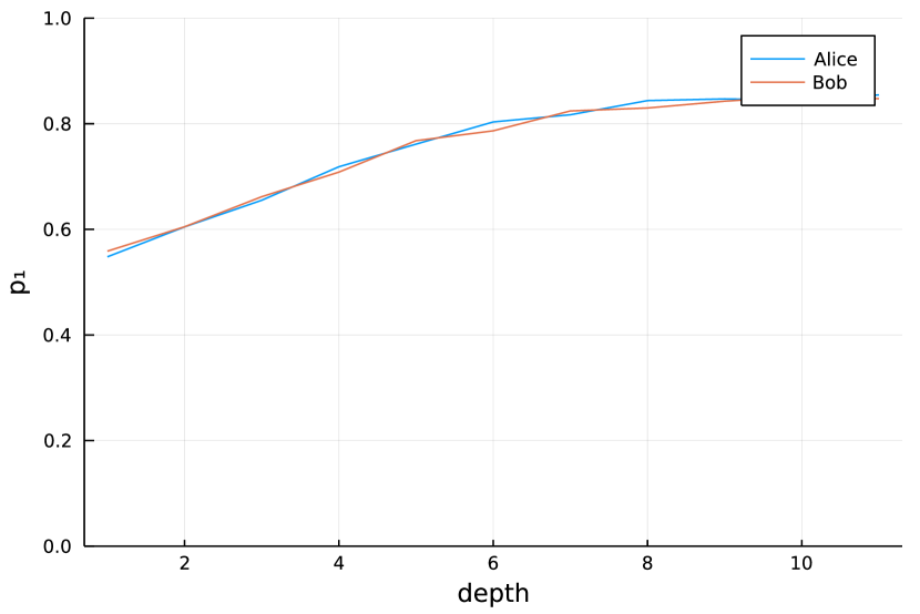
(a) Monte Carlo approximation

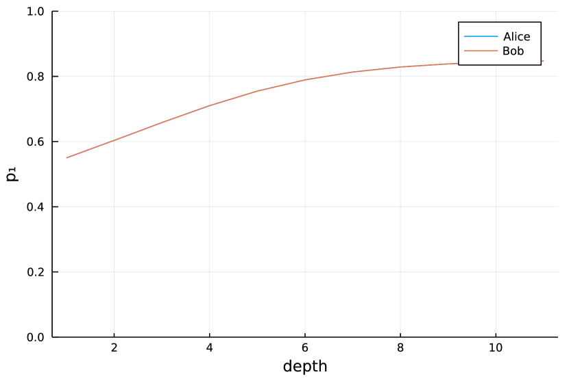
(b) Analytical solution

Figure 1: Bob and Alice like the same bar: $p_{Alice}^{1}=p_{Bob}^{1}=0.55$, $p_{Alice}^{m}=p_{Bob}^{m}=0.9$

Figure 2 addresses contradictory preferences with respect to bars — Alice strongly prefers the first bar, while Bob slightly prefers the second bar. Since they still want to meet, they both choose, when the deliberation depth is sufficient, the first bar more often than the second one.

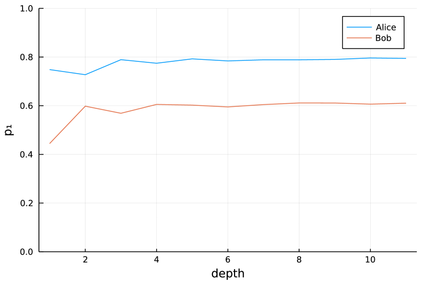
(a) Monte Carlo approximation

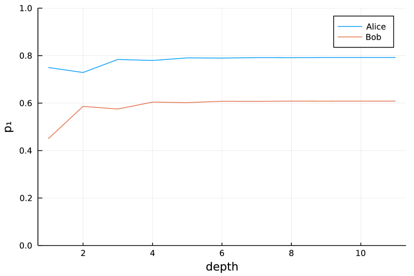
(b) Analytical solution

Figure 2: Bob and Alice like different bars: $p_{Alice}^{1}=0.75$, $p_{Bob}^{1}=0.45$, $p_{Alice}^{m}=p_{Bob}^{m}=0.75$

9.1.2 Bob Chases Alice, Alice Avoids Bob

Another setting is an instance of pursuit-evasion game: Bob chases Alice, but Alice avoids Bob. The choice distributions of both agents depend on how strong their preferences to meet, or to avoid the meeting, are. Figure 3 shows inference results for the case where Bob’s and Alice’s feelings are opposite but mild. As Bob and Alice deliberate deeper and deeper, their choice distributions eventually converge to stable limits.

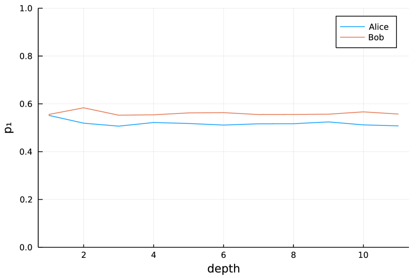
(a) Monte Carlo approximation

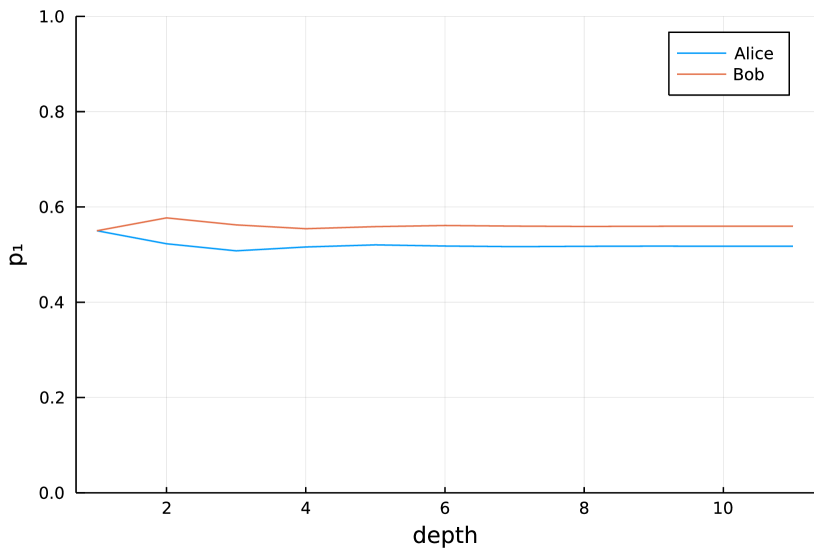
(b) Analytical solution

Figure 3: Bob chases Alice, mild feelings: $p_{Alice}^{1}=p_{Bob}^{1}=0.55$, $p_{Alice}^{m}=0.25$, $p_{Bob}^{m}=0.75$

However, if Bob’s and Alice’s feelings are opposite and strong (Figure 4), the agents overthink and act impulsively — as the deliberation depth increases, the choice distributions of both agents alternate between going to the first or to the second bar with increasing probability.

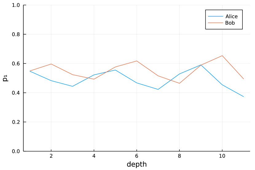
(a) Monte Carlo approximation

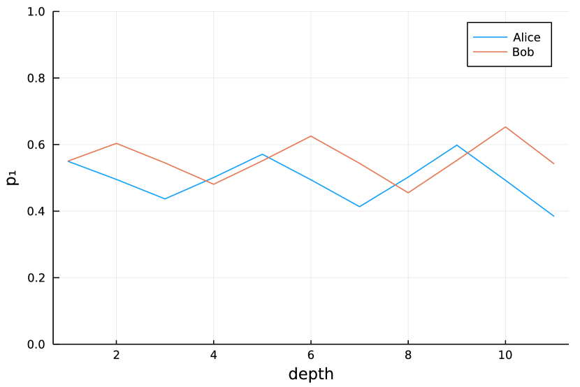
(b) Analytical solution

Figure 4: Bob chases Alice, strong feelings: $p_{Alice}^{1}=p_{Bob}^{1}=0.55$, $p_{Alice}^{m}=0.1$, $p_{Bob}^{m}=0.9$

9.1.3 Bob and Alice Avoid Each Other

Further on, we explore the case when Bob and Alice avoid each other, that is, both of them would rather go to the pub where they are unlikely to meet the other person. When the preference towards avoiding is mild (Figure 5), Bob and Alice, with sufficient deliberation depth, approach their prior preferences, that is they both go to the first bar with the probability approaching $p_{Alice}^{1}=p_{Bob}^{1}$. Indeed, rationally this the best they can do to minimize their chances to meet each other without coordination, while still respecting their preference of the first bar.

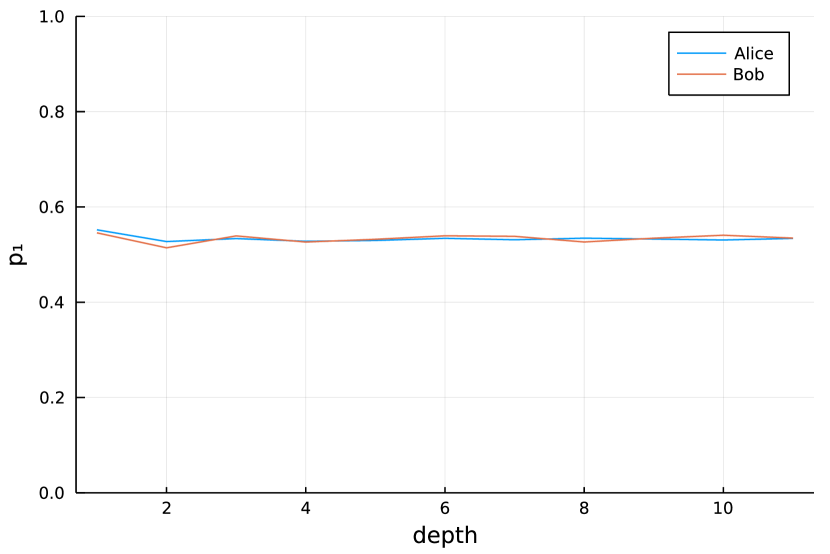
(a) Monte Carlo approximation

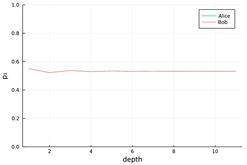
(b) Analytical solution

Figure 5: Bob and Alice avoid each other, mild feelings: $p_{Alice}^{1}=p_{Bob}^{1}=0.55$, $p_{Alice}^{m}=p_{Bob}^{m}=0.25$

However, when Bob’s and Alice’s mutual despisal is too strong (Figure 6), mutual epistemic reasoning does a poor job — Bob and Alice switch their increasingly strong posterior preferences between the first and the second bar with each level of deliberation depth, similarly to the case of strong feelings in pursuit-evasion situation. One may argue that these outcomes are algorithmically anomalous, or ‘irrational’; however, they may be also interpreted as a demonstration that rational behavior is not unconditionally stable, and cannot be guaranteed for arbitrary combinations of preferences.

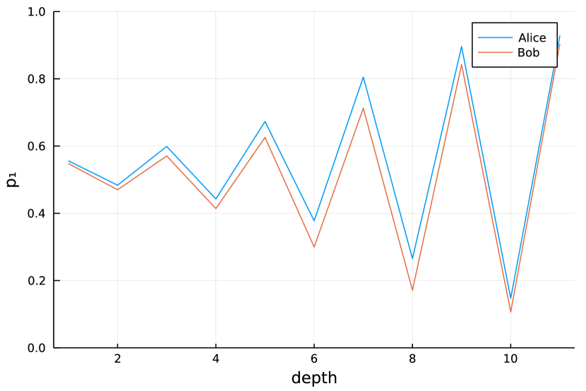
(a) Monte Carlo approximation

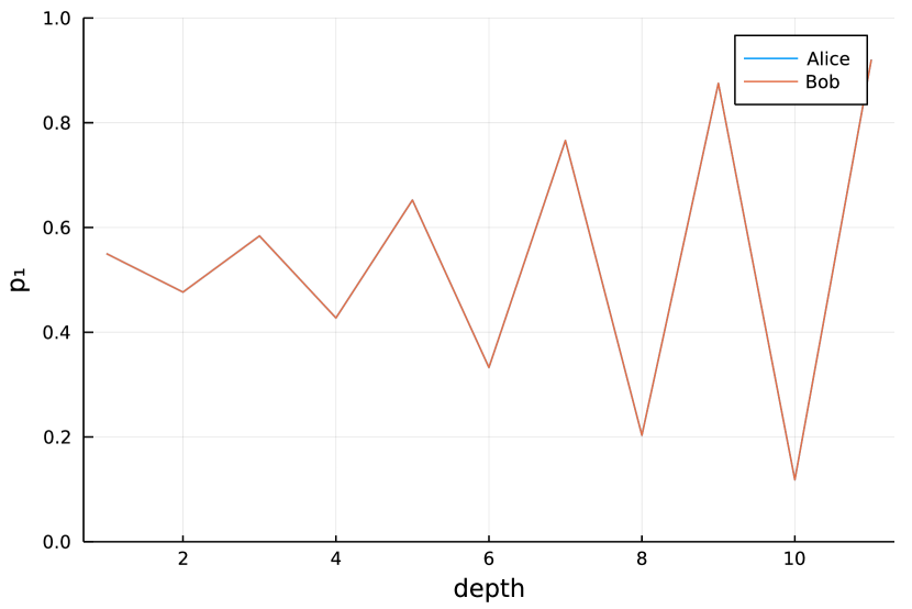
(b) Analytical solution

Figure 6: Bob and Alice avoid each other, strong feelings: $p_{Alice}^{1}=p_{Bob}^{1}=0.55$, $p_{Alice}^{m}=p_{Bob}^{m}=0.05$

9.1.4 Alice Learns Bob’s Preferences

Finally, let us see how Alice can find out whether Bob wants to meet her by observing Bob’s behavior. We use the same model of Alice for inference, but instead of conditioning the model on Bob’s preferences, we condition the model on the history of Bob’s choices and infer Bob’s preference (log-odds) of meeting Alice. We condition the model on three Bob’s choices in a row, and compare Alice’s conclusions for two cases:

1. Bob chose the first bar three times in a row;

2. Bob chose the second bar three times in a row.

To visualize the results, we draw 100 samples from the posterior distribution of the probability with that Bob would choose to meet Alice everything else being equal. Figure 7 shows a two-dimensional scatter plot where each direction is the marginal distribution of log-odds of Bob willing to meet Alice. Indeed, 96 out of 100 points are below the diagonal, meaning that Alice can be very confident that Bob is willing to meet her if she observes Bob in the first bar 3 times in a row. However, if Bob shows up three times in a row in the second bar, Alice should conclude that Bob is avoiding her.

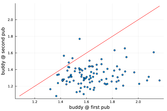
Figure 7: Alice infers Bob preferences: three visits to the same bar in a row provide strong evidence about Bob’s desire to meet Alice.

9.2 The Sailing Problem

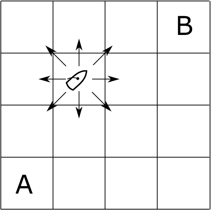
(a) lake

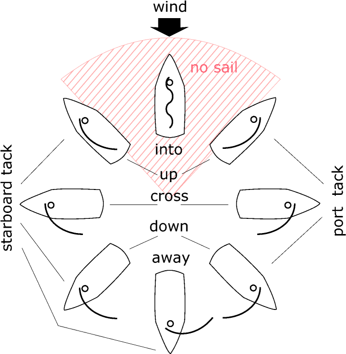
(b) points of sail

Figure 8: The sailing problem

The sailing problem (Figure 8) is a popular benchmark problem for search and planning. A sailing boat must travel between the opposite corners A and B of a square lake of a given size. At each step, the boat can head in 8 directions (legs) to adjacent squares (Figure 8(a)). The unit distance cost of movement depends on the wind (Figure 8(b)), which can also blow in 8 directions. There are five relative boat and wind directions and associated costs: into, up, cross, down, and away. The cost of sailing into the wind is prohibitively high, upwind is the highest feasible, and away from the wind is the lowest. The side of the boat off which the sail is hanging is called the tack, either port or starboard. When the angle between the boat and the wind changes sign, the sail must be tacked to the opposite tack, which incurs an additional tacking delay cost. The objective is to find a policy that minimizes the expected travel cost. The wind is assumed to follow a random walk, either staying the same or switching to an adjacent direction, with a known probability.

Table 1: Sailing problem parameters

cost						wind probability
into	up	cross	down	away	delay	same	left	right
$\infty$	4	3	2	1	4	0.4	0.3	0.3

For any given lake size, there is a non-parameteric stochastic policy that tabulates the distribution of legs for each combination of location, tack, and wind. However, such policy does not generalize well — if the lake area increases, due to a particularly rainy year for example, the policy is not applicable to the new parts of the lake. In this case study, we infer instead a generalizable parametric policy balancing between hesitation in anticipation for a better wind and rushing to the goal at any cost. The policy chooses a leg with the log-probability equal to the euclidian distance between the position after the log and the goal, multiplied by the policy parameter $\theta$ (the leg directed into the wind is excluded from choices). The greater the $\theta$, the higher is the probability that a leg bringing the boat closer to the goal will be chosen:

$$\log\Pr({\operatorname{\mathit{leg}}})=\theta\cdot{\operatorname{\mathit{distance}}}({\operatorname{\mathit{next-location}}},{\operatorname{\mathit{goal}}})-\log Z$$ (10)

here, $Z$ is the normalization constant ensuring that the probabilities of all legs sum up to 1. It can be readily computed but is not required for inference. We implemented the model and inference in Infergo [Tol19].

The model turns out to be similar in structure to that of Bob and Alice.

• The first agent, Alice, is the boat. The agent chooses a path across the lake.

• The second agent, Bob, is the wind. The agent chooses a random walk of wind direction along the boat’s path. The wind is a neutral agent — it does not try to either help or tamper with the boat.

• The boat’s path, stochastically conditioned on the wind, has the probability proportional to the product of exponentiated negated leg costs (which are interpreted as negated log probabilities of the boat to choose each leg regardless of the goal location).

Model (11) formalizes our setting:

$${\operatorname{\mathit{wind-history}}}\sim{\operatorname{\mathit{RandomWalk}}}$$ (11)

$$\log\theta\sim\mathrm{Uniform(0,\infty)}$$

$${\operatorname{\mathit{boat-trajectory}}}\sim D({\operatorname{\mathit{wind-history}}},\theta)$$

$$\Pr({\operatorname{\mathit{boat-trajectory}}},\theta)\propto\exp(-{\operatorname{\mathit{travel-cost}}}({\operatorname{\mathit{boat-trajectory}}},{\operatorname{\mathit{wind-history}}}))$$

The model parameters (cost and wind change probabilities), same as in [KS06, TS12], are shown in Table 1. A non-informative improper prior is imposed on $\theta$. We fit the model using pseudo-marginal Metropolis-Hastings [AR09] and used $10\,000$ samples to approximate the posterior. Figure 9 shows the posterior distribution of the unit cost. Table 2 shows the expected travel costs, with the expectations estimated both over the unit cost and the wind. The inferred travel costs are compared to the travel costs of the ‘optimal’ policy and of the greedy policy, according to which the boat always heads in the direction of the steepest decrease of the distance to the goal. One can see that the inferred policy attains an expected travel cost lying between the greedy policy and the ‘optimal’ policy, as one would anticipate.

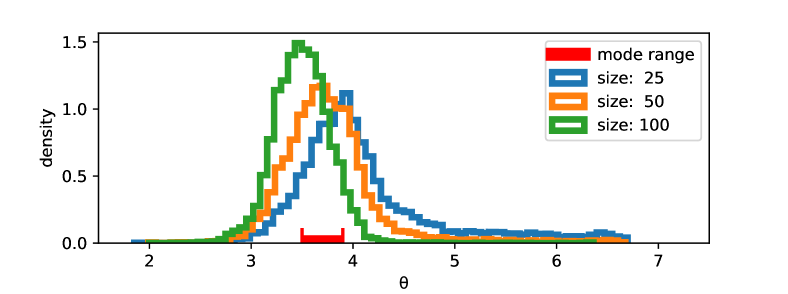
Figure 9: The sailing problem: $\theta$

Table 2: The sailing problem: travel cost

	25	50	100
Inferred	105	209	413
Greedy	107	215	430
Optimal	103	206	406

10 Related Work

Possibility and importance of casting reinforcement learning as probabilistic inference are well understood in AI research [TS06, BA09]. [KZT11] explore planning as inference in the case of multiple agents, exploring special cases in which efficient scalable inference is possible.

Although not strictly in the field of reinforcement learning, [Kap07] lays out stochastic control theory and shows the connection between Boltzmann distribution and expected utility maximization. [WGR⁺11] demonstrates usefulness and applicability of probabilistic programming for planning as inference on deterministic planning domains. [vdMPTW16] apply probabilistic programming to stochastic domains, using a custom policy search algorithm.

[SG14] explore multiagent settings using probabilistic programming, implementing theory of mind through mutually recursive nested condition of models. [SvdMW18] apply theory of mind using probabilistic programming to an elaborated pursuit-evasion problem.

[TZRY21] introduces stochastic conditioning, a Bayesian inference formalism necessary to cast reinforcement learning as a purely probabilistic Bayesian inference problem. In one of the case studies, [TZRY21] provide an early indication that planning as inference can be implemented through stochastic conditioning.

11 Discussion

We demonstrated that reinforcement learning, that is, agent’s reasoning about preferred future behavior, can be formulated as Bayesian inference. Probability distributions can be used to specify all aspects of uncertainty or stochasticity, including agent preferences. Rewards can be interpreted as log-odds of stochastic preferences and do not need to be explicitly introduced. Planning algorithms maximizing the expected utility find maximum a posteriori characterization of the rational policy distribution.

References

- [AN04] Pieter Abbeel and Andrew Y. Ng. Apprenticeship learning via inverse reinforcement learning. In Proceedings of the Twenty-First International Conference on Machine Learning, ICML ’04, page 1, New York, NY, USA, 2004. Association for Computing Machinery.
- [AR09] Christophe Andrieu and Gareth O. Roberts. The pseudo-marginal approach for efficient Monte Carlo computations. The Annals of Statistics, 37(2):697–725, 2009.
- [BA09] Matthew Botvinick and Ja/mes An. Goal-directed decision making in prefrontal cortex: a computational framework. In D. Koller, D. Schuurmans, Y. Bengio, and L. Bottou, editors, Advances in Neural Information Processing Systems, volume 21. Curran Associates, Inc., 2009.
- [CTSLM19] Marco F. Cusumano-Towner, Feras A. Saad, Alexander K. Lew, and Vikash K. Mansinghka. Gen: A general-purpose probabilistic programming system with programmable inference. In Proceedings of the 40th ACM SIGPLAN Conference on Programming Language Design and Implementation, PLDI 2019, page 221–236, New York, NY, USA, 2019. Association for Computing Machinery.
- [ESSF17] Owain Evans, Andreas Stuhlmüller, John Salvatier, and Daniel Filan. Modeling Agents with Probabilistic Programs. http://agentmodels.org, 2017. Accessed: 2021-7-29.
- [HFWL17] Xiao Huang, Biqing Fang, Hai Wan, and Yongmei Liu. A general multi-agent epistemic planner based on higher-order belief change. In Proceedings of the Twenty-Sixth International Joint Conference on Artificial Intelligence, IJCAI-17, pages 1093–1101, 2017.
- [HGEJ17] Ahmed Hussein, Mohamed Medhat Gaber, Eyad Elyan, and Chrisina Jayne. Imitation learning: A survey of learning methods. ACM Comput. Surv., 50(2), April 2017.
- [Kap07] Hilbert J. Kappen. An introduction to stochastic control theory, path integrals and reinforcement learning. In American Institute of Physics Conference Series, volume 887, pages 149–181, 2007.
- [KG15] Filippos Kominis and Hector Geffner. Beliefs in multiagent planning: From one agent to many. ICAPS’15, page 147–155. AAAI Press, 2015.
- [KS06] Levente Kocsis and Csaba Szepesvári. Bandit based Monte-Carlo planning. In Proceedings of the European Conference on Machine Learning, pages 282–293, 2006.
- [KZT11] Akshat Kumar, Shlomo Zilberstein, and Marc Toussaint. Scalable multiagent planning using probabilistic inference. In Proceedings of the Twenty-Second International Joint Conference on Artificial Intelligence - Volume Volume Three, IJCAI’11, page 2140–2146. AAAI Press, 2011.
- [Noz69] Robert Nozick. Newcomb’s Problem and Two Principles of Choice, pages 114–146. Springer Netherlands, Dordrecht, 1969.
- [NR00] Andrew Y. Ng and Stuart J. Russell. Algorithms for inverse reinforcement learning. In Proceedings of the Seventeenth International Conference on Machine Learning, ICML ’00, page 663–670, San Francisco, CA, USA, 2000. Morgan Kaufmann Publishers Inc.
- [PG04] Laurent Péret and Frédérick Garcia. On-line search for solving Markov decision processes via heuristic sampling. In Proceedings of the 16th European Conference on Artificial Intelligence, pages 530–534, 2004.
- [PM17] David L. Poole and Alan K. Mackworth. Artificial Intelligence: Foundations of Computational Agents. Cambridge University Press, USA, 2nd edition, 2017.
- [Rai18] Tom Rainforth. Nesting probabilistic programs. In Proceedings of the 34th Conference on Uncertainty in Artificial Intelligence, pages 249–258, 2018.
- [SG14] A. Stuhlmüller and N.D. Goodman. Reasoning about reasoning by nested conditioning: Modeling theory of mind with probabilistic programs. Cognitive Systems Research, 28:80–99, 2014. Special Issue on Mindreading.
- [SvdMW18] Iris Rubi Seaman, Jan-Willem van de Meent, and David Wingate. Nested reasoning about autonomous agents using probabilistic programs, 2018.
- [Sze10] Csaba Szepesvári. Algorithms for reinforcement learning. Synthesis Lectures on Artificial Intelligence and Machine Learning, 4(1):1–103, January 2010.
- [Tol99] Eckhart Tolle. The power of now: a guide to spiritual enlightenment. Novato, California: New World Library, 1999.
- [Tol19] David Tolpin. Deployable probabilistic programming. In Proceedings of the 2019 ACM SIGPLAN International Symposium on New Ideas, New Paradigms, and Reflections on Programming and Software, pages 1–16, 2019.
- [TS06] Marc Toussaint and Amos Storkey. Probabilistic inference for solving discrete and continuous state markov decision processes. In Proceedings of the 23rd International Conference on Machine Learning, ICML’06, page 945–952, New York, NY, USA, 2006. Association for Computing Machinery.
- [TS12] David Tolpin and Solomon Eyal Shimony. MCTS based on simple regret. In Proceedings of The 26th AAAI Conference on Artificial Intelligence, pages 570–576, 2012.
- [TZRY21] David Tolpin, Yuan Zhou, Tom Rainforth, and Hongseok Yang. Probabilistic programs with stochastic conditioning. In Marina Meila and Tong Zhang, editors, Proceedings of the 38th International Conference on Machine Learning, volume 139 of Proceedings of Machine Learning Research, pages 10312–10323. PMLR, 18–24 Jul 2021.
- [vdMPTW16] Jan-Willem van de Meent, Brooks Paige, David Tolpin, and Frank Wood. Black-box policy search with probabilistic programs. In Proceedings of the 19th International Conference on Artificial Intelligence and Statistics, pages 1195–1204, 2016.
- [vdMPYW18] Jan-Willem van de Meent, Brooks Paige, Hongseok Yang, and Frank Wood. An introduction to probabilistic programming. arXiv:1809.10756, 2018.
- [WGR+11] David Wingate, Noah D. Goodman, Daniel M. Roy, Leslie P. Kaelbling, and Joshua B. Tenenbaum. Bayesian policy search with policy priors. In Proceedings of the 22nd International Joint Conference on Artificial Intelligence, pages 1565–1570, 2011.