Evaluation of distortion correction methods in diffusion MRI of the spinal cord

Abstract

Background: Magnetic field inhomogeneities generate important geometric distortions in reconstructed echo-planar images. Various procedures were proposed for correcting these distortions on brain images; yet, few neuroimaging studies tailored and incorporated the use of these techniques in spinal cord diffusion MRI.
Purpose: We present a comparative evaluation of distortion correction methods that use the reversed gradient polarity technique on spinal cord. We propose novel geometric metrics to measure the alignment of the reconstructed diffusion model with the apparent centerline of the spinal cord.
Subjects: 95 subjects, among which 29 healthy controls and 66 multiple sclerosis patients.
Sequence: 3T, diffusion-weighted echo-planar imaging of the spinal cord, b-value 900s/mm², 30 directions.
Assessment: Geometric distortions were corrected using 4 state-of-the-art methods. We measured the alignment of the principal direction of diffusion with the apparent centerline of the spine after correction and the correlation with the reference anatomical image. Results are computed per vertebral level, to evaluate the impact on different portions of the spine. Besides, a global, subjective evaluation of the quality of the correction of healthy subjects images was performed by three expert raters.
Statistical tests: A paired Tukey test associated to no difference between metrics from the non-corrected data and metrics from each of the 4 correction methods were computed. A logistic model including a rater effect was fitted to the subjective evaluation data.
Results: As a result of distortion correction, the diffusion directions are better aligned locally with the centerline ($p<0.05$), in particular at both ends of the acquisition window. The cross-correlation with anatomical image is also improved by HySCO ($p=2.10^{-4}$) and block-matching ($p=0.029$). The subjective evaluation for HySCO is significantly better (p < 0.05) than for Block-Matching; TOPUP performs significantly worse than the three other methods.
Data Conclusions: Correction based on Hyperelastic Susceptibility Artefact Correction (HySCO) provide best results among the selected methods.

Keywords: diffusion MRI, distortion correction, echo-planar imaging, spinal cord imaging.

1 Introduction

Echo-Planar-Imaging (EPI) is a fast and efficient magnetic resonance imaging (MRI) acquisition technique [1] useful for diffusion-weighted MRI. It is however sensitive to the $B_{0}$ field inhomogeneities, caused by the local susceptibility variations in the human body. In this respect, in vivo spinal cord imaging is especially challenging due to the presence of various surrounding tissues and environments: bone, cerebrospinal fluid (CSF), gray and white matter, muscle, fat and air. Besides, the elongated shape of the spinal cord anatomy requires a large field of view in the superior-inferior direction and its small cross-sectional size requires high spatial resolution. These requirements extend the readout durations in EPI which in turn distorts and blurs the image along the phase-encoding direction (PED). Also, a large echo-spacing, the interval between two consecutive line readouts in $k$-space, creates distortions due to $B_{0}$ field inhomogeneity.

Geometric distortions affect the reconstructed image so that a voxel normally at position $\mathbf{r}$ appears at a position $\mathbf{r}+\mathbf{d_{\mathrm{PED}}}(\mathbf{r})$. This displacement, $\mathbf{d_{\mathrm{PED}}}(\mathbf{r})$, occurs mainly in the PED and is negligible in other directions [2, 3]. Depending on parameters of the EPI sequence such as the echo spacing, the field of view in the PED and the $B_{0}$ field inhomogeneity), the magnitude of the displacements can reach up to 60 mm [4] in typical spinal cord images (6ppm off-resonance at 3T, field of view of $18\text{\,}\mathrm{cm}$ in the PED and echo-spacing of $0.5\text{\,}\mathrm{ms}$) need to be addressed carefully before analysis. In addition to the spatial distortion presented above, there also is an intensity distortion in EPI [2].

Various acquisition-based optimizations have been proposed to reduce susceptibility artifacts for spinal cord imaging [4]. In addition, there is a number of distortion correction techniques, including co-registration, field map correction, point spread function (PSF) and reversed gradient polarity method (RGP). Most of these techniques require an additional specific acquisition and are based on the distortion model derived in [5].

First, among these techniques, co-registration uses a non distorted anatomical image, typically a T₂-weighted acquisition as a reference. Applying non-linear registration, a displacement field is computed to warp the non diffusion-weighted image to the T₂-weighted image. The same transform is then applied to the diffusion-weighted images prior to diffusion model fitting. In general, imaging protocols do include an anatomical scan so this technique does not increase the overall acquisition time. However, this technique is sensitive to the quality of the registration, a task which can be challenging due to differences in contrast and field of view between the diffusion and the anatomical image.

The second technique, field map correction, relies on a 2 minutes acquisition of a double-echo gradient-echo sequence, from which a $B_{0}$ field map is reconstructed [2, 6]. This map is in turn used to generate a warping field which will be applied to the EPI series. This technique is convenient, but is sensitive to subject motion during acquisition as well as large local variations in the magnetic field [7, 8]. Post-processing using this kind of acquisition is implemented in FSL and Statistical Parametric Mapping (SPM) toolbox.

Another technique [9, 10] also relies on the acquisition of an extra dedicated sequence from which the point spread function of the system is estimated. The technique can be accelerated using parallel imaging [11, 12]. The point spread function mapping captures both intensity and geometric distortions induced by field inhomogeneity. Applying this technique to diffusion MRI of the spinal cord [13] was proven effective in recovering large distortion, thus enabling fiber tractography in the cervical region.

The last technique, commonly referred to as reversed gradient polarity (RGP), uses two EPI acquired with the same field of view and matrix size, but in opposite phase encoding direction [5]. The apparent displacements in these reconstructed images are of the same magnitude but have opposite directions. One can exploit this to compute the corresponding displacement map using both images as input: the corrected image is therefore midway between the two distorted acquisitions. Some studies consider this technique as an alternative to field map correction as the field map here is implicitly estimated using an additional EPI. This RGP technique is distinctive by requiring only a quick additional EPI acquisition to correct distortion, if we consider that acquiring only the non diffusion-weighted image in reverse PED is sufficient. Furthermore, Cohen-Adad et al. shown its potential for the correct estimation of both geometric and intensity distortion as compared to PSF, field map and co-registration [14].

In this work, we focus on the evaluation of post-processing distortion correction techniques using the RGP technique. We propose a comparative evaluation of post-processing methods using the pair of acquisitions for the correction of geometric distortions. We first give an overview of the state-of-the-art methods we will evaluate. Then, we introduce a new geometric measure of alignment between the centerline of the spinal cord and the reconstructed principal direction of diffusion. Finally, we compare these methods on a database of 95 subjects (29 healthy controls and 66 multiple sclerosis patients) using the newly introduced measure of alignment, together with a comparison to the anatomical T2-weighted image using cross-correlation and mutual information. In addition to these objective evaluations, a subjective comparison of the images corrected with each of the 4 methods was performed by 3 independent raters. To the best of our knowledge, this is the first time such a comparison of these methods, otherwise designed for brain imaging, is made for spinal cord imaging.

2 Materials and methods

2.1 Distortion correction from RGP technique

A range of post-processing methods have been proposed for the estimation and the correction of geometric distortions in EPI from a pair of acquisitions with RGP. In this work we compare 4 such distortion correction methods: block-matching (BM) [15], hyper-elastic susceptibility artefact correction (HySCO) [16], TOPUP [7] and Voss [17]. In this section, we first present the physical model common to all methods, then we give an overview of the image processing methodology for each.

Distortion model

A pair of spin-echo EPI are acquired in reversed phase encoding directions, in our case head-feet (HF) and feet-head (FH), which correspond to the $y$-axis. Let $I_{F}$ denote the forward gradient EPI image, acquired traversing $k$-space in the positive $y$-direction (HF), and $I_{B}$ (for backward) the reverse gradient image acquired traversing in the negative $y$-direction FH. The corrected image $I_{C}$ is therefore midway between $I_{F}$ and $I_{B}$. The problem is to find the deformation field from $I_{F}$ (or equivalently from $I_{B}$) to $I_{C}$ [15].

Method 1: Block-Matching

The block-matching (BM) strategy looks for a transformation by finding a local correspondence between small blocks (typically $3\times 3\times 3$ voxels) in the original and the target image [18, 19]. This method, applied to field inhomogeneity-induced distortion correction in EPI [15], follows the registration method introduced in [20]. BM [15] adapts the approach to block matching algorithm presented by [18, 19] by constraining the transform to be aligned with the PED, using a cross-correlation metric as a measure of similarity. BM method is implemented and available in Anima, an open-source software for medical image processing.

Method 2 : HySCO

The Hyper-elastic Susceptibility artefact COrrection method (HySCO) [16, 3] is based on the physical distortion model derived in [5]. HySCO estimates the displacement $b:\Omega\to\mathbb{R}$ by minimizing the following distance functional:

$$\mathcal{D}[b]=\frac{1}{2}\int_{\Omega}\left(I_{F}(\mathbf{x}+b(\mathbf{x})\mathbf{v})(1+\mathbf{v}^{\top}\nabla b(\mathbf{x}))-I_{B}(\mathbf{x}-b(\mathbf{x})\mathbf{v})(1-\mathbf{v}^{\top}\nabla b(\mathbf{x}))\right)^{2}\mathrm{d}\mathbf{x}$$ (1)

where $\mathbf{v}$ denotes the PED, $\mathbf{v}=(0,1,0)^{\top}$, $\Omega$ the rectangular region of interest, $b(\mathbf{x})$ is the magnitude of the field inhomogeneity at $\mathbf{x}\in\Omega$. Since minimizing $\mathcal{D}$ is an ill-posed problem, HySCO introduces the following regularization:

$$\mathcal{S}(b)=\frac{1}{2}\int_{\Omega}\left\|\nabla b(\mathbf{x})\right\|^{2}\mathrm{d}x.$$ (2)

HySCO is implemented as a part of ACID toolbox and integrated as a batch tool in the Statistical Parametric Mapping (SPM).

Method 3: TOPUP

Similarly, TOPUP [7] takes as input two images with opposite PEDs and jointly estimates a displacement field map and an undistorted image using least squares, to be used to reconstruct the undistorted image. TOPUP is implemented and distributed as part of the FSL package . Notice that when applying TOPUP algorithm on data, extreme slices of image volume are collapsed. We applied TOPUP with its default parameters except for resampling, we used the Jacobian method.

Method 4: Voss

Voss et al. [17] proposed a distortion correction method to reduce geometric and intensity distortions. For each image coordinates $x$ and $z$, this method seeks to align the corresponding line in the forward and backard images at coordinates $x,\cdot,z$. Note that this method realigns each line independently, so in order to increase the coherence between adjacent lines, a 3D Gaussian smoothing is applied to the deformation. This method is implemented and available in Anima. We used the method with default parameters in our comparison.

2.2 Geometric measure of alignment

In order to evaluate the impact of geometric distortion correction, we introduce in this section a measure of alignment between the geometry of the spinal cord, represented by its centerline, and the principal direction of diffusion. In previous studies [13, 17, 14], one of the criteria used for the evaluation or the validation of distortion-correction was to use fiber tractography in the spinal cord. We hypothesize that measuring the alignment of the diffusion direction and the spinal cord geometry is an alternative, more direct way to evaluate the consistency between the diffusion anisotropy and the underlying image geometry.

The diffusion tensor model relates the local displacement of water molecules with the surrounding tissue microstructure. In the spinal cord white matter, it is mainly aligned with longitudinal fibers [21], which themselves follow a path parallel to the centerline of the spinal cord. We can therefore expect that the principal eigenvector of the diffusion tensor is locally aligned tangentially with the centerline of the spinal cord. However, when the image is distorted, the apparent shape of the spinal cord is affected, while the direction of the tensor is not. This results in a local misalignment of the diffusion tensor with the spinal cord (see Figure.1). In what follows, we describe a method to measure how the diffusion tensors and the centerline of spinal cord align with each other.

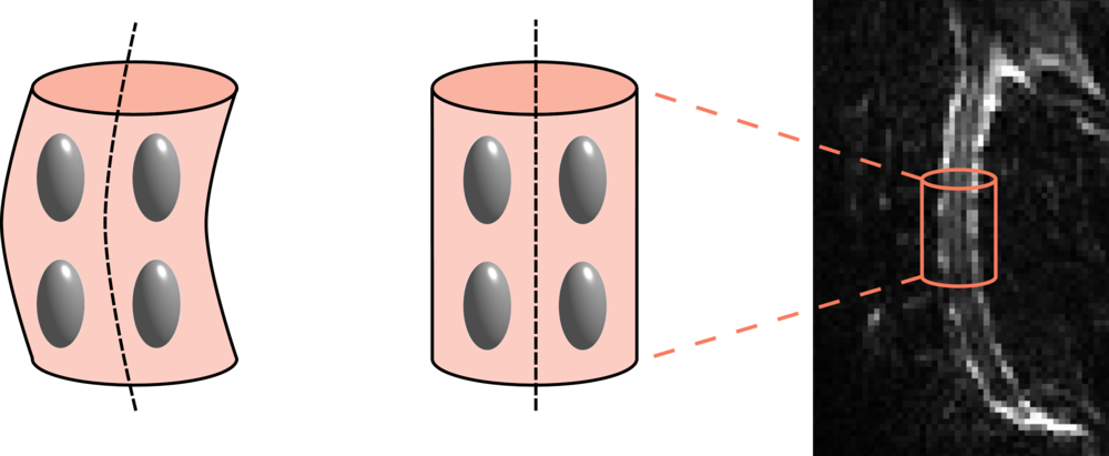
Figure 1: Illustration of the diffusion tensor field within the spinal cord: distorted image (left), undistorted (middle). The principal direction of diffusion is not affected by distortion, as a result it appears misaligned with the centerline of the spine on the distorted image (left).

Centerline extraction and modeling

We first segment the diffusion image to obtain a binary mask of the spinal cord using the spinal cord toolbox (SCT) [22, 23]. This segmentation is computed from the mean diffusion-weighted images. Using this binary mask of the spinal cord, we compute the centerline in two steps: first, for every axial slice, we compute the barycenter of the mask within this slice; then we fit a degree-3 smoothing spline to the set of barycenters, using UnivariateSpline provided in SciPy with default smoothing parameter. This provides us with a continuous, differentiable representation of the centerline as a parametric equation of variable $t$, from which we can compute the Frenet frame at every point of the centerline.

Local frame attached to the spine centerline

Let $\mathbf{x}(t)\in\mathbb{R}^{3}$ be a curve parametrized by $t\in\mathbb{R}^{+}$. Also, let $\mathbf{v(t)}=\mathbf{x(t)}^{\prime}$ denotes the velocity. We define the curvilinear abscissa $s$ as:

$$s(t)=\int_{0}^{t}|\mathbf{x}^{\prime}(\tau)|\mathrm{d}\tau,$$ (3)

The Frenet frame is defined as the triplet $(\mathbf{t},\mathbf{n},\mathbf{b})$ where $\mathbf{t}$ is the tangent, $\mathbf{n}$ the normal and $\mathbf{b}$ the binormal (see Figure.2) defined as

$$\mathbf{t}=\frac{\mathbf{v(t)}}{\|\mathbf{v(t)}\|};\quad\mathbf{n}=\frac{\mathbf{t}^{\prime}}{\|\mathbf{t}\|};\qquad\mathbf{b}=\frac{\mathbf{t}\times\mathbf{n}}{\|\mathbf{t}\times\mathbf{n}\|}.$$

Measuring the alignment of the diffusion model with the cord

For every voxel at position $\mathbf{r}$ within the spinal cord, we first compute the closest point $\mathbf{x}(t_{0})$ to $\mathbf{r}$ along the centerline where $t_{0}$ is by minimizing (with an exhaustive grid search):

$$t_{0}=\arg\min_{t}\{||\mathbf{x}(t)-\mathbf{r}||\}.$$ (4)

Then we compute the coordinates of the principal eigenvector of the diffusion tensor, $\mathbf{e}_{1}(\mathbf{r})$, in the Frenet frame computed at $\mathbf{x}(t_{0})$.

In order to summarize the distribution of the principal eigenvectors $\mathbf{e}_{1}(\mathbf{r})$ within a region $\Omega$, we compute the covariance matrix of these directions [24] as follows:

$$\mathbf{M}=\frac{1}{\mathcal{V}(\Omega)}\int_{\Omega}\mathbf{e}_{1}(\mathbf{r})\mathbf{e}_{1}(\mathbf{r})^{\top}\mathrm{d}\mathrm{r}$$ (5)

where $\mathcal{V}(\Omega)$ is the volume of $\Omega$. Intuitively, the matrix $\mathbf{M}$ will characterize the statistics of the angular deviation between the diffusion direction and the tangent to the centerline. From the eigendecomposition of the symmetric matrix, $\mathbf{M}$, we extract two statistics:
Mean angle direction (MAD): defined as the angle in degrees between the principal eigenvector of $\mathbf{M}$ and [1,0,0], which corresponds to $\mathbf{T}$ in the Frenet frame
Angular concentration of directions (ACD): defined as the first eigenvalue of $\mathbf{M}$. Being the average of rank-1 non-negative symmetric matrices with eigenvalues (1,0,0), $\mathbf{M}$ has eigenvalues in the range of [0,1]. The more concentrated around the mean direction, the closer to 1 is the ACD.

These statistics were computed for $\Omega\in\{$Brain stem, C1, …, C7, T1, T2$\}$ corresponding to every cervical and thoracic vertebral levels in the acquisition window.

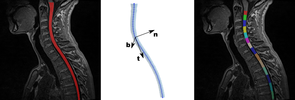
Figure 2: (left) T1 image with segmented spinal cord for reference; (middle) 3d representation of the segmented spine, smoothed centerline (blue solid line) and the Frenet frame at a particular point of the centerline; (right) registration of the PAM50 template to identify intervertebral levels of the spine.

2.3 Imaging data

Data used in this evaluation were acquired on 3T scanners (Magnetom Verio and Skyra, Siemens Healthineers, Erlangen) at four sites in France: Marseille, Rennes, Strasbourg and Montpellier as part of the EMISEP project .

Patients and healthy volunteers

Twenty nine healthy volunteers (mean age = 32.83$\pm$7.13, 18F/11M) and 66 MS patients (mean age = 32.20$\pm$6.30, 42F/24M) were recruited in the study after approval from the institutional review board. MS patients are early relapsing-remitting MS patients (scan within the first year following diagnosis), with a median Expanded Disability Status Scale (EDSS) score of 1.0 (range [0, 2.5]). All participants provided informed written consent. Table. 1 illustrates more details about MRI scanners, centers and demographics.

Center	Marseille	Rennes	Strasbourg	Montpellier	TOTAL
3T scanner MRI	Verio	Verio	Verio	Skyra	-
Volunteers	4	18	3	4	29
Gender	1F/3M	10F/8M	3F	4F	18F/11M
MS Patients	7	44	8	7	66
Gender	4F/3M	28F/16M	5F/3M	5F/2M	42F/24M
					95 (60F/35M)

Table 1: Demographic information for all participating subjects, healthy controls and MS patients from several centers and total study cohort.

MRI data acquisition

EMISEP PHRC protocol includes Diffusion-weighted imaging scan: Thirty non-collinear diffusion-weighted images (DWI) were acquired at $b=900$ s$\cdot$mm^-2, six non-DWI ($b=0$) measurements and one non-DWI ($b=0$s/mm²) with an opposite phase encoding direction (PED) were also acquired. This was repeated three times successively in order to increase the signal-to-noise ratio (SNR). Scans were performed in sagittal orientation and head-feet (HF) PED to cover the whole cervical cord. The pulse sequence used for diffusion MRI was a single-shot Echo-planar imaging (ss-EPI) using parallel imaging (GRAPPA, acceleration factor 2). Sixteen slices were acquired with the following parameters without inter-slice gap: TR/TE = 3600/90 ms, with 2x2x2 mm³ as the resolution, and image matrix 80x80. The total acquisition time for the DWI sequence was approximately 7 minutes. The protocol also includes the following two high-resolution images for anatomical reference. Firstly, T₁-weighted scan: in sagittal orientation, magnetization-prepared rapid acquisition gradient echo (3D MPRAGE) sequence with an isotropic 1x1x1 mm³ resolution, TR/TI/TE = 1800/900/2.79 ms, flip angle 9^∘ and FoV = 250$\times$250 mm², 64 slabs. Secondly, T₂-weighted scan: in sagittal orientation, 2D Turbo Spin Echo, with anisotropic 0.7x0.7x2.75 mm³ resolution, TR/TE = 3000/68.0 ms and FoV = 260$\times$260 mm², 15 slices with 2.5 mm slice thickness and 10% gap between slices.

2.4 MRI pre-processing

Motion correction

The diffusion-weighted volumes were re-aligned to compensate for subject motion during the 7 minutes acquisition. Since motion is often observed within the axial plane [25], the correction were carried out allowing only rigid slice-wise transformations in the axial plane using the spinal cord toolbox (SCT) version 3.0b4 [26, 27]. This way of realigning all volumes was shown to be robust and accurate [25].

Distortion correction

Then, diffusion-weighted data were corrected for susceptibility distortion using the four cited methods: Block-Matching (BM) available in Anima, HySCO as implemented in SPM-ACID toolbox, TOPUP implemented in FSL and Voss method implemented in Anima. We computed a displacement field using one non-DWI ($b=0$) for each PED. Then, this displacement was applied to the whole set of diffusion-weighted volumes. We refer to the diffusion-weighted images after distortion correction as "corrected DWI".

Segmentation of the cord and identification of vertebral level

Using SCT [27], whole spinal cord segmentation was carried out on T₁-weighted, on T₂-weighted, on the corrected by each method and uncorrected DWI (b = 900 s$\cdot$mm^-2) averaged across all gradient directions. Then, we identify manually two vertebral levels, C3 and T1 since this manual step is recommended in the SCT for an accurate registration to the PAM50 template.

Quality Control

To ensure that the results are immune to image artefacts, and to identify problems during the processing pipelines, we performed a careful quality control (QC) on the raw data and after each processing step. We eliminated 7 subjects which contained too many artifacts not apparently related to B₀-field inhomogeneity (motion and ghosting).

2.5 Computing geometric metrics by vertebral level

Here, our aim is to compute statistics on geometric measures, MAD and ACD, for each vertebral level. To do so, we register the PAM50 template [28] and the T₁-weighted anatomical data and the mean diffusion-weighted image. Firstly, T₁-weighted anatomical data were registered to the PAM50 spinal cord template [28]. This generates forward and inverse warping fields from one to the other. Next, we register the PAM50-T1 template [28] to the mean DWI using the inverse warping field from the previous step as an initial warping field. Then, using the registered template, we compute the proposed geometric metrics as explained in 2.2 within each vertebral level.

Here, we preferred to use T₁-weighted image rather than the T₂-weighted since the former has isotropic resolution, which makes the registration more effective. Alignment with the template provides robust definition of the inter-vertebral levels for the spinal cord. This enables computation of the average metrics in spinal cord using the atlas-based approach introduced in [29]. As a result, we can quantify the geometric diffusion-based metrics averaged for each inter-vertebral level from C1 to T2. The processing pipeline is summarized in Figure. 3.

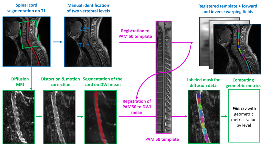
Figure 3: Illustration of the automated analysis pipeline. (1) Segmentation of the cord on T₁-weighted. (2) Manual identification of two vertebral levels. (3) Registration to the PAM50 template. (4) Motion and distortion correction of DWI. (5) Segmentation of the cord using DWI mean data. (6) Registration of PAM50-T1 registered to DWI mean data using the inverse warping field from previous registration as an initial warping field. (7) Computing MAD and ACD by vertebral level of the cervical part.

2.6 Computing cross-correlation and mutual information

Complementary to the geometric measure of alignment, we also compute the similarity between the corrected $b=0$ image and the T₂-weighted image. Firstly, we rigidly registered T₂-weighted scan to the first $b=0$ volume of the uncorrected and corrected DWI. We then apply this rigid transform to the binary mask of the spinal cord obtained by segmenting the T₂-weighted image, which is now warped to the first $b=0$ volume of the uncorrected and DWI. Finally, we compute the cross-correlation (CC) and mutual information (MI) between the T2-weighted image and the $b=0$ volume only within the spinal cord region. The cross-correlation, also referred to as Pearson correlation coefficient, is a measure of the linear correlation between two variables $x$ and $y$. This coefficient has a value in $[-1,1]$, where -1 and 1 are total negative and positive linear correlation respectively and 0 is no linear correlation. This coefficient is commonly represented by $r_{xy}$ and defined as:

$$\mathit{r_{xy}}=\frac{\sum_{i=1}^{n}(x_{i}-x_{m})(y_{i}-y_{m})}{\sqrt{\sum_{i=1}^{n}(x_{i}-x_{m})^{2}\sum_{i=1}^{n}(y_{i}-y_{m})^{2}}}$$ (6)

where $n$ is the size of the mask in voxels, $x_{i}$ and $y_{i}$ are the intensities at voxel $i$ of the T₂-weighted and DWI, $x_{m}$ and $y_{m}$ are their sample mean over the same ROI. The mutual information (MI) is a measure of the mutual dependence between two variables $x$ and $y$. It quantifies the amount of information obtained about $x$ through observing $y$. MI of $x$ and $y$ is given as:

$$\mathit{MI(x,y)}=\sum_{i=1}^{n}\sum_{i=1}^{n}p(x_{i},y_{i})~{}log\left(\frac{p(x_{i},y_{i})}{p(x_{i})p(y_{i})}\right),$$ (7)

where $p(x,y)$ is the joint probability function of $x$ and $y$, and $p(x)$ and $p(y)$ are the marginal probability distribution functions of $x$ and $y$, respectively.

2.7 Subjective evaluation

Three experts (E.B, S.L and A.K) compared the resulting mean diffusivity (MD) images obtained after applying each of the four distortion correction methods described above on the 29 healthy volunteers in the database. Using a web-based interface implemented internally, the raters were provided with the images corrected using each method side-by-side, along with the non-corrected image. The raters were asked to rank the four corrected images, based on their subjective appreciation of the resulting image. The methods were unknown to the raters and the order in which images were presented were shuffled randomly for every subject. The ranks were exported to a CSV file and analyzed with R.

3 Results

3.1 Geometric statistics

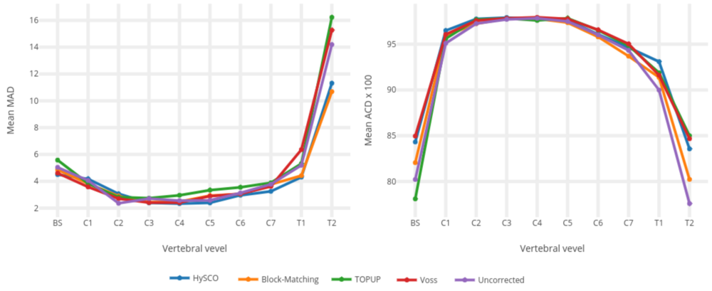
Figure 5: Mean MAD (in degrees) and mean ACD ($\times$ 100) reported by vertebral level. This way of representation shows that extreme vertebral level of the acquisition window are more affected by distortion.

For every distortion correction method, geometric statistics were computed for every cervical and thoracic levels in the acquisition window. Results of mean and standard deviation of each metric, MAD and ACD, for brain stem (BS) and each vertebral level are presented in tables  2 and  3. For each level, the adjusted p-values associated to no difference between metrics from the non-corrected data and metrics from each of the 4 correction methods were computed using a paired Tukey test. Figure. 5 shows the MAD and ACD by vertebral level; vertebral levels located at the end of the acquisition window are more affected by distortion. Note that MAD is a measure of the bias in the orientation, which means that a decrease in MAD should be interpreted as an improvement in the alignment. By contrast, ACD is a measure of angular dispersion, and an increase in ACD is considered as an improvement.

3.2 Subjective comparison

The relative performance of each correction method with respect to the others is summarized in 4. Moreover, for each pair of methods, a logistic model including a random rater-effect was fitted and the p-value for "log-odd=0" (i.e. in average method 1 performs better than method 2 in half of all virtually possible cases) was computed and reported.

3.3 Comparison with anatomical images

Since the T₂-weighted image is not affected by distortion, it can be considered as a gold-standard for the evaluation of distortion correction. So, we also compare the corrected volume ($b=0$s/mm²) of DWI by each method to the T₂-weighted image. We report results of cross-correlation and mutual information. Note that results presented here are slightly different to the study reported in [30] since the treatment pipeline and datasets are different. A paired Tukey test was performed on the cross-correlation scores and reported in Table. 5 and on the mutual information scores and reported in Table. 6.

3.4 Vertebral level volume

Last, we computed the volume in mm³ of each vertebral level for uncorrected and corrected data as shown in Table. 7. This table contains also results of paired Tukey test to compare the volume of each method to the non-corrected DWI.

4 Discussion

In this work, we have proposed novel geometric diffusion-based metrics and framework for studying the impact of distortion correction in diffusion MRI of the spinal cord. We showed a difference in geometric alignment after correcting with one method or another.

For HySCO method, as shown in Table. 2, we can observe that MAD metric performs significantly better than uncorrected in T1 and T2 vertebral levels. But, this method has significant deterioration at C2 vertebral level, as BM, but mean MAD of HySCO is more close to the uncorrected. For ACD metric, we remark a significant improvement at edges of the spinal cord (brain stem, C1, C7 and T1 regions) as shown in Table. 3. Last, we note as shown in Table.4 that HySCO performs significantly better in the subjective evaluation than BM and TOPUP.

For Block-Matching method, as shown in Table. 2, we observe that it performs significantly better in T1 vertebral levels. However, there is a significant deterioration in C2. For ACD metric, BM improves the concentration significantly in brain stem region, C1, C2, T1 and T2. We note also as shown in Table. 4 that BM performs significantly better in the subjective evaluation than TOPUP.

For Voss method, we observe a significant improvement in MAD metric for C1 vertebral level and significant deterioration in T1 vertebral level. But, there is a very remarkable amelioration for ACD in all vertebral levels, except C3 and C4 which are in the middle of the field-of-view of the acquisition. Last, we note as shown in Table. Table. 4 that Voss performs significantly better in the subjective evaluation than TOPUP. However, TOPUP method is recognized as the major method for the postprocessing distortion correction of diffusion MRI data [31, 32].

For TOPUP method, we consider significant deterioration in MAD in C2 and C5 vertebral levels without any significant improvement. For ACD metric, there is significant improvement at C2, C5, C6 and T2 vertebral levels. Last, we note as shown in Table. 4 that TOPUP performs significantly worse in the subjective evaluation than the other 3 methods.

Complementary to the geometric measure of alignment, we also compute the similarity between the corrected $b=0$ image and the T₂-weighted image. For cross-correlation, there is a significant amelioration only for Block-Matching and HySCO as demonstrated in Table. 5. For mutual information, there is a significant amelioration for all methods as shown in Table. 6. Last, we compared the apparent volume of each vertebral level before and after applying each distortion correction method (results reported in Table. 7. We note that all methods have a significant impact on the volume, which is related to the specific implementation of the distortion correction and interpolation methods. Despite having no ideal method to evaluate these changes, we decided to report them here, since they vary from one method to another.

4.1 Conclusion

We proposed a framework to evaluate distortion correction methods applied to diffusion MRI of the spinal cord. The results of objective and subjective evaluation on a database of 95 subjects show that among these methods, HySCO stands out in its ability to reduce the bias in diffusion direction (MAD) after distortion correction and in the subjective evaluation by experts. A possible next step in this research will be to incorporate this notion of alignment as a constraint to design a new correction algorithm tailored to spine diffusion MR images.

Mean Angle Direction (MAD)
	Block-Matching		HySCO		TOPUP		Voss		Uncorrected
Level	Mean	STD	Mean	STD	Mean	STD	Mean	STD	Mean	STD
BS	4.50	3.59	4.86	3.48	5.58	4.61	4.61	3.76	5.04	3.94
C1	4.18	5.75	3.83	3.89	3.84	2.39	3.58	2.89	4.06	2.83
C2	3.07	1.98	2.90	2.04	2.82	1.70	2.71	2.01	2.36	1.44
C3	2.39	1.64	2.44	1.55	2.74	1.75	2.41	1.56	2.71	1.61
C4	2.34	1.91	2.49	1.82	2.96	1.81	2.41	1.63	2.56	1.71
C5	2.39	1.61	2.93	2.29	3.34	2.13	2.89	1.77	2.58	1.44
C6	2.96	2.10	3.06	2.04	3.55	2.16	3.07	2.26	3.13	2.13
C7	3.25	2.82	3.77	3.83	3.89	3.50	3.62	4.08	3.78	3.21
T1	4.31	4.40	4.42	4.25	5.32	7.59	6.36	6.20	5.19	4.64
T2	11.31	10.72	10.68	10.05	16.22	17.43	15.26	12.28	14.19	14.76

Table 2: Mean and standard deviation for Mean Angle Direction (MAD) metric in degrees for data corrected by Block-Matching, HySCO, TOPUP and Voss and uncorrected data.light green means that p-value shows significant improvement with $10^{-3}<$ p-value $<5.10^{-2}$, weak red means that p-value shows significant deterioration. BS: brain stem.

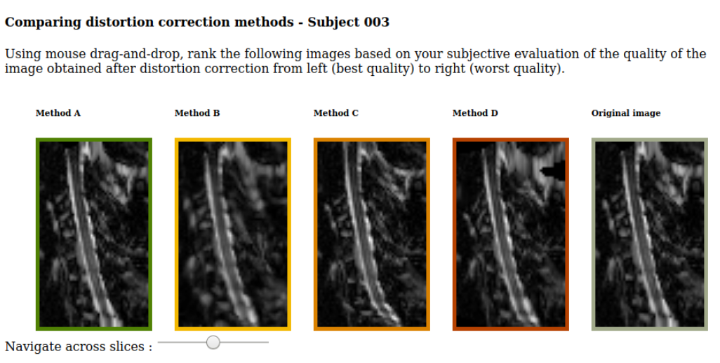
Figure 4: Screenshot of the web interface for expert ranking. The images corrected using each of the four method are presented side-by-side, along with the original image. The order in which the methods are displayed is shuffled randomly for each subject, and the methods are labeled neutrally as "Method A", "Method B", …, etc.

Angular Concentration of directions (ACD)
	Block-Matching		HySCO		TOPUP		Voss		Uncorrected
Level	Mean	STD	Mean	STD	Mean	STD	Mean	STD	Mean	STD
BS	84.32	8.66	82.06	8.57	78.10	9.46	84.96	8.01	80.22	8.71
C1	96.49	4.96	95.93	4.56	95.60	5.84	96.06	3.92	95.10	5.76
C2	97.75	2.14	97.23	2.29	97.68	2.20	97.57	2.21	97.25	2.55
C3	97.91	2.08	97.80	2.01	97.82	1.89	97.83	2.23	97.71	2.23
C4	97.73	2.34	97.77	1.82	97.59	2.33	97.93	1.57	97.83	1.69
C5	97.62	1.68	97.35	2.06	97.83	1.64	97.76	1.44	97.48	1.63
C6	96.08	4.03	95.80	3.75	96.53	3.56	96.57	3.19	96.02	3.31
C7	94.63	6.17	93.69	6.52	94.84	7.44	95.03	5.05	94.32	6.08
T1	93.09	7.92	91.37	7.49	91.88	9.17	91.61	7.70	89.99	9.58
T2	83.56	12.66	80.23	14.47	85.00	13.99	84.67	11.40	77.59	16.15

Table 3: Mean and standard deviation multiplied by $\mathbf{10^{2}}$ for ACD metric for data corrected by Block-Matching, HySCO, TOPUP and Voss and uncorrected data.Dark green means that p-value shows significant improvement with p-value $<\mathrm{1}0^{-3}$,light green means that p-value shows also significant improvement but $10^{-3}<$ p-value $<5.10^{-2}$. BS: brain stem.

	Voss	BM	TOPUP
HySCO	41 vs 46 (p=0.72)	49 vs 28 (p=0.0019)	76 vs 11 (p=$3.10^{-5}$)
Voss	NA	59 vs28 (p=0.14)	77 vs 10 (p=0.0027)
BM	NA	NA	67 vs 20 (p=0.01)

Table 4: Summary of the pairwise logistic regression (accounting for a random rater effect): we report for each pair of methods the score for method 1 (row) vs method 2 (column). For instance, among the 87 subjective evaluations (29 subjects, 3 raters), Voss ranked behind HySCO 41 times.

Cross-correlation
Methods	BM	HySCO	TOPUP	Voss	Uncorrected
Mean	0.185	0.242	0.179	0.148	0.160
STD	0.114	0.119	0.150	0.115	0.107
P-value	0.029	2.10-4	0.189	0.173	-
t-statistic	2.215	7.303	1.325	-1.375	-

Table 5: Paired Tukey test for Block-Matching, HySCO, TOPUP and Voss for Cross-correlation for the whole of the spinal cord region. Dark green means that p-value shows significant improvement and inferior to $\mathrm{1}0^{-3}$, light green means that p-value shows significant improvement but $10^{-3}<$ p-value $<5.10^{-2}$.

Mutual information
Methods	BM	HySCO	TOPUP	Voss	Uncorrected
Mean	0.304	0.330	0.312	0.293	0.277
STD	0.051	0.049	0.064	0.053	0.054
P-value	10-5	4.10-14	6.10-7	9.10-4	-
t-statistic	4.652	9.198	5.433	3.449	-

Table 6: Paired Tukey test for Block-Matching, HySCO, TOPUP and Voss for Mutual information for the whole of the spinal cord region. Dark green means that p-value shows significant improvement and inferior to $\mathrm{1}0^{-3}$, light green means that p-value shows significant improvement but $10^{-3}<$ p-value $<5.10^{-2}$.

	BM		HySCO		TOPUP		Voss		Uncorrected
Level	Mean	STD	Mean	STD	Mean	STD	Mean	STD	Mean	STD
C1	560.5	123	583.9	106	555.9	118	555.8	110	568.7	104
C2	530.7	118	552.0	101	528.7	123	526.8	103	538.7	108
C3	913.2	155	967.6	165	911.5	173	934.8	146	917.8	155
C4	959.8	157	1021	163	923.0	175	949.4	142	943.4	152
C5	855.4	158	901.6	150	823.3	170	837.3	143	835.5	150
C6	777.3	137	810.8	126	725.1	161	753.7	141	749.6	134
C7	743.6	127	764.4	120	681.7	134	710.4	132	732.6	127
T1	790.4	138	820.9	153	722.3	158	742.8	173	757.6	158
T2	456.9	277	501.0	283	363.7	265	339.5	283	397.9	271

Table 7: Volume of every vertebral level (in mm³) of spinal cord, segmented mask, corrected by Block-Matching, HySCO, TOPUP, Voss and uncorrected. Significant differences ($p<0.05$) are indicated by blue color.

References

- Stehling et al. [1991] Stehling MK, Turner R, Mansfield P. Echo-planar imaging: magnetic resonance imaging in a fraction of a second. Science 1991;254(5028):43–50.
- Jezzard and Balaban [1995] Jezzard P, Balaban RS. Correction for geometric distortion in echo planar images from B0 field variations. Magnetic resonance in medicine 1995;34(1):65–73.
- Macdonald and Ruthotto [2016] Macdonald J, Ruthotto L. Efficient numerical optimization for susceptibility artifact correction of EPI-MRI. arXiv preprint arXiv:160700531 2016;.
- Saritas et al. [2014] Saritas EU, Holdsworth SJ, Bammer R. Susceptibility artifacts. In: Cohen-Adad J, Wheeler-Kingshott C, editors. Quantitative MRI of the Spinal Cord Elsevier; 2014.p. 91–105.
- Chang and Fitzpatrick [1992] Chang H, Fitzpatrick JM. A technique for accurate magnetic resonance imaging in the presence of field inhomogeneities. IEEE Transactions on medical imaging 1992;11(3):319–329.
- Reber et al. [1998] Reber PJ, Wong EC, Buxton RB, Frank LR. Correction of off resonance-related distortion in echo-planar imaging using EPI-based field maps. Magnetic Resonance in Medicine 1998;39(2):328–330.
- Andersson et al. [2003] Andersson JL, Skare S, Ashburner J. How to correct susceptibility distortions in spin-echo echo-planar images: application to diffusion tensor imaging. Neuroimage 2003;20(2):870–888.
- Holland et al. [2010] Holland D, Kuperman JM, Dale AM. Efficient correction of inhomogeneous static magnetic field-induced distortion in Echo Planar Imaging. Neuroimage 2010;50(1):175–183.
- Robson et al. [1997] Robson MD, Gore JC, Constable RT. Measurement of the point spread function in MRI using constant time imaging. Magnetic resonance in medicine 1997;38(5):733–740.
- Zeng and Constable [2002] Zeng H, Constable RT. Image distortion correction in EPI: comparison of field mapping with point spread function mapping. Magnetic Resonance in Medicine: An Official Journal of the International Society for Magnetic Resonance in Medicine 2002;48(1):137–146.
- Zaitsev et al. [2004] Zaitsev M, Hennig J, Speck O. Point spread function mapping with parallel imaging techniques and high acceleration factors: fast, robust, and flexible method for echo-planar imaging distortion correction. Magnetic Resonance in Medicine: An Official Journal of the International Society for Magnetic Resonance in Medicine 2004;52(5):1156–1166.
- Speck et al. [2008] Speck O, Stadler J, Zaitsev M. High resolution single-shot EPI at 7T. Magnetic Resonance Materials in Physics, Biology and Medicine 2008;21(1-2):73.
- Lundell et al. [2013] Lundell H, Barthelemy D, Biering-Sørensen F, Cohen-Adad J, Nielsen JB, Dyrby TB. Fast diffusion tensor imaging and tractography of the whole cervical spinal cord using point spread function corrected echo planar imaging. Magnetic resonance in medicine 2013;69(1):144–149.
- Cohen-Adad et al. [2009] Cohen-Adad J, Lundell H, Rossignol S. Distortion correction in spinal cord DTI: what’s the best approach. In: Proceedings of the 17th Annual Meeting of ISMRM, Honolulu, USA, vol. 3178; 2009. .
- Hedouin et al. [2017] Hedouin R, Commowick O, Bannier E, Scherrer B, Taquet M, Warfield SK, et al. Block-Matching Distortion Correction of Echo-Planar Images With Opposite Phase Encoding Directions. IEEE Trans Med Imaging 2017;36(5):1106–1115.
- Ruthotto et al. [2012] Ruthotto L, Kugel H, Olesch J, Fischer B, Modersitzki J, Burger M, et al. Diffeomorphic susceptibility artifact correction of diffusion-weighted magnetic resonance images. Physics in Medicine & Biology 2012;57(18):5715.
- Voss et al. [2006] Voss HU, Watts R, Uluğ AM, Ballon D. Fiber tracking in the cervical spine and inferior brain regions with reversed gradient diffusion tensor imaging. Magnetic resonance imaging 2006;24(3):231–239.
- Ourselin et al. [2000] Ourselin S, Roche A, Prima S, Ayache N. Block matching: A general framework to improve robustness of rigid registration of medical images. In: International Conference on Medical Image Computing And Computer-Assisted Intervention Springer; 2000. p. 557–566.
- Commowick et al. [2012] Commowick O, Wiest-Daesslé N, Prima S. Automated diffeomorphic registration of anatomical structures with rigid parts: Application to dynamic cervical MRI. In: International Conference on Medical Image Computing and Computer-Assisted Intervention Springer; 2012. p. 163–170.
- Avants et al. [2008] Avants BB, Epstein CL, Grossman M, Gee JC. Symmetric diffeomorphic image registration with cross-correlation: evaluating automated labeling of elderly and neurodegenerative brain. Medical image analysis 2008;12(1):26–41.
- Cohen-Adad et al. [2008] Cohen-Adad J, Descoteaux M, Rossignol S, Hoge RD, Deriche R, Benali H. Detection of multiple pathways in the spinal cord using q-ball imaging. Neuroimage 2008;42(2):739–749.
- De Leener et al. [2014] De Leener B, Kadoury S, Cohen-Adad J. Robust, accurate and fast automatic segmentation of the spinal cord. Neuroimage 2014;98:528–536.
- De Leener et al. [2015] De Leener B, Cohen-Adad J, Kadoury S. Automatic segmentation of the spinal cord and spinal canal coupled with vertebral labeling. IEEE transactions on medical imaging 2015;34(8):1705–1718.
- Mardia and Jupp [2009] Mardia KV, Jupp PE. Directional statistics, vol. 494. John Wiley & Sons; 2009.
- Mohammadi et al. [2013] Mohammadi S, Freund P, Feiweier T, Curt A, Weiskopf N. The impact of post-processing on spinal cord diffusion tensor imaging. Neuroimage 2013;70:377–385.
- Xu et al. [2013] Xu J, Shimony JS, Klawiter EC, Snyder AZ, Trinkaus K, Naismith RT, et al. Improved in vivo diffusion tensor imaging of human cervical spinal cord. Neuroimage 2013;67:64–76.
- De Leener et al. [2017] De Leener B, Lévy S, Dupont SM, Fonov VS, Stikov N, Collins DL, et al. SCT: Spinal Cord Toolbox, an open-source software for processing spinal cord MRI data. Neuroimage 2017;145:24–43.
- De Leener et al. [2018] De Leener B, Fonov VS, Collins DL, Callot V, Stikov N, Cohen-Adad J. PAM50: Unbiased multimodal template of the brainstem and spinal cord aligned with the ICBM152 space. NeuroImage 2018;165:170–179.
- Lévy et al. [2015] Lévy S, Benhamou M, Naaman C, Rainville P, Callot V, Cohen-Adad J. White matter atlas of the human spinal cord with estimation of partial volume effect. Neuroimage 2015;119:262–271.
- Snoussi et al. [2017] Snoussi H, Caruyer E, Commowick O, Bannier E, Barillot C. Comparison of inhomogeneity distortion correction methods in diffusion MRI of the spinal cord. In: ESMRMB-34th Annual Scientific Meeting; 2017. .
- Dauleac et al. [2021] Dauleac C, Bannier E, Cotton F, Frindel C. Effect of distortion corrections on the tractography quality in spinal cord diffusion-weighted imaging. Magnetic Resonance in Medicine 2021;.
- Hu et al. [2020] Hu Z, Wang Y, Zhang Z, Zhang J, Zhang H, Guo C, et al. Distortion correction of single-shot EPI enabled by deep-learning. NeuroImage 2020;221:117170.