Prescribed-Time Regulation of Nonlinear Uncertain Systems with Unknown Input Gain and Appended Dynamics

Abstract

The prescribed-time stabilization problem for a general class of nonlinear systems with unknown input gain and appended dynamics (with unmeasured state) is addressed. Unlike the asymptotic stabilization problem, the prescribed-time stabilization objective requires convergence of the state to the origin in a finite time that can be arbitrarily picked (i.e., prescribed) by the control system designer irrespective of the initial condition of the system. The class of systems considered is allowed to have general nonlinear uncertain terms throughout the system dynamics as well as uncertain appended dynamics (that effectively generate a time-varying non-vanishing disturbance signal input into the nominal system). The control design is based on a time scale transformation, dynamic high-gain scaling, and adaptation dynamics with temporal forcing terms.

I Introduction

While the stabilization/regulation objective typically considered in control designs [1, 2, 3, 4] is formulated in term of asymptotic convergence (as time $t\rightarrow\infty$) of the state to a desired state value (e.g., the origin), the control objective of “finite-time” stabilization [5, 6, 7, 8, 9, 10, 11, 12, 13, 14, 15] addresses the possibility of achieving the desired convergence properties over a finite time interval. The length of this finite time interval that is attained depends, in general, on the system dynamics and the initial conditions. Requiring this finite time interval to be a constant that is independent of the initial condition, i.e., requiring that the convergence should be attained within a fixed terminal time that is independent of initial condition, yields the stronger control objective of “fixed-time” stabilization [16, 12, 17, 18, 19, 20]. Further requiring that the fixed finite time should be a parameter that can be arbitrarily “prescribed” by the control designer irrespective of the initial condition yields the even stronger control objective of “prescribed-time” stabilization [21, 22, 23, 24, 25, 26, 27, 28, 29, 30, 31, 32, 33, 34, 35].

To force convergence within the specified finite prescribed time, two general prescribed-time stabilizing controller design approaches that have been addressed in the literature can be viewed as state scaling or time scaling:

• State scaling by a time-dependent function [21, 22, 28]: By, for example, scaling the state $x$ to define $\tilde{x}=\mu(t)x$ where $\mu(t)$ is a “blow-up” function defined such that $\mu(t)\rightarrow\infty$ as $t\rightarrow T$, a control design that keeps $\tilde{x}$ bounded will implicitly make $x$ go to 0 as $t\rightarrow T$.

• Time scaling using a nonlinear temporal transformation [31, 32, 33, 34, 35]: Define, for example, $\tau=a(t)$ with $a$ being a function defined such that $a(0)=0$ and $\lim_{t\rightarrow T}a(t)=\infty$. Since this time scale transformation maps $t\in[0,T)$ to $\tau\in[0,\infty)$, a control design that achieves asymptotic convergence in terms of the time variable $\tau$ implicitly achieves prescribed-time convergence in terms of the time variable $t$.

The state scaling approach has been applied in [21, 22, 28] to design prescribed-time stabilizing controllers for classes of systems such as chains of integrators with uncertainties matched with the control input (i.e., normal form). Prescribed-time stabilizing controllers have been designed for nonlinear strict-feedback-like systems [31, 32, 33, 34, 35] using the time scaling approach to convert the prescribed-time stabilization problem into an asymptotic stabilization problem in terms of the transformed time variable and applying the dual dynamic high gain scaling based observer-controller design techniques [36, 37, 38, 39, 40, 41, 42, 43] to achieve asymptotic stabilization in terms of the transformed time variable. While [31] considered the prescribed-time stabilization problem under state feedback, output feedback was addressed in [32]. The adaptation of the control design techniques from [36, 37, 38, 39, 40, 41, 42, 43] that were originally developed in the context of asymptotic stabilization to the prescribed-time context necessitated introduction of time-dependent forcing terms into the high-gain scaling parameter dynamics and a set of modifications in the controller design and the Lyapunov analysis to achieve prescribed-time convergence instead of asymptotic convergence. Uncertain nonlinear systems with general structures of uncertain functions throughout the system dynamics including combinations of unknown parameters (without requiring any known magnitude bounds on unknown parameters) and unmeasured state variables were addressed in [33] and a dynamic output-feedback prescribed-time stabilizing controller was developed. A partial state-feedback prescribed-time stabilizing controller was designed for systems with uncertainties in the input gain and non-vanishing input-matched disturbances in addition to uncertain terms throughout the system dynamics in [34]. An output-feedback prescribed-time stabilizing controller was designed for systems with time delays of unknown magnitude in [35].

Based on the prescribed-time stabilizing control design in [34], we consider in this paper a general class of nonlinear systems that include an unknown input gain and time-varying non-vanishing disturbances generated by an uncertain appended dynamics in addition to nonlinear time-varying uncertain terms throughout the system dynamics. The uncertain terms in the system dynamics are allowed to contain both parametric and functional uncertainties without requiring magnitude bounds on the uncertain parameters. Specifically, we consider a class of nonlinear systems of the following form:

$$\dot{x}_{i} =\phi_{i}(z,x,u,t)+\phi_{(i,i+1)}(x,t)x_{i+1}\ \ ,i=1,\ldots,n-1$$

$$\dot{x}_{n} =\phi_{n}(z,x,u,t)+h(z,x,u,t)u$$

$$\dot{z} =q(z,x,u,t)$$ (1)

where $x=[x_{1},\ldots,x_{n}]^{T}\in{\mathcal{R}}^{n}$ is the state of the nominal system, $z=[z_{1},\ldots,z_{n_{z}}]^{T}\in{\mathcal{R}}^{n_{z}}$ is the state of an appended dynamics coupled with the $x$ subsystem, and $u\in{\mathcal{R}}$ is the input. $\phi_{(i,i+1)},i=1,\ldots,n-1$ are known scalar real-valued continuous functions. $\phi_{i},i=1,\ldots,n$, $h$, and $q$ are time-varying scalar real-valued uncertain functions of their arguments. The state $x$ of the nominal system is measured while the state $z$ of the appended dynamics is assumed to be unmeasured. The uncertain function $h$ represents the unknown control input gain, which is allowed to be time-varying and state-dependent. Furthermore, while $h$ is assumed to have known sign (without loss of generality, assumed positive) and lower-bounded in magnitude by a non-zero constant (to ensure controllability), the lower bound is not required to be known unlike [34]. The bounds imposed on functions $\phi_{i}(z,x,u,t)$ in the assumptions on the system structure in Section II allow these functions to depend nonlinearly on the entire system state $x$ as well as appearance of an uncertain parameter $\theta$ (without requirement for a known magnitude bound) and coupling with the state of the appended dynamics. Furthermore, the bound on $\phi_{n}(z,x,u,t)$ is allowed to contain an additive term that is not required to go to 0 when the state approaches the origin, i.e., a non-vanishing disturbance. A known upper bound on this non-vanishing disturbance is not required unlike [34]. It will be seen in the control design and stability and convergence analysis in Sections III and IV that prescribed-time stabilization can be attained for the considered class of systems through several novel ingredients including non-smooth components in the control law, temporal forcing terms in the adaptation dynamics and the scaling parameter dynamics, interconnections between the adaptation dynamics and the scaling parameter dynamics taking into account the time scale transformation $t\rightarrow\tau$, and analysis of the closed-loop system properties.

This paper is organized as follows. The assumptions imposed on the system (1) are provided in Section II. The control design is presented in Section III. The main result of the paper is presented in Section IV. Concluding remarks are contained in Section VI.

II Notations, Control Objective, and Assumptions

Notations:

• The notation $|a|$ denote Euclidean norm of a vector $a$ or absolute value of a scalar $a$. The notation $||M||$ denotes Frobenius norm of a matrix $M$.

• The notation $\mbox{diag}(T_{1},\ldots,T_{m})$ denotes an $m\times m$ diagonal matrix with diagonal elements $T_{1},\ldots,T_{m}$. Also, $\mbox{lowerdiag}(T_{1},\ldots,T_{m-1})$ and $\mbox{upperdiag}(T_{1},\ldots,T_{m-1})$ denote the $m\times m$ matrices with the lower diagonal entries (i.e., entries at locations $(i+1,i)$ for $i=1,\ldots,m-1$) and upper diagonal entries (i.e., entries at locations $(i,i+1)$ for $i=1,\ldots,m-1$), respectively, being $T_{1},\ldots,T_{m-1}$ and zeros everywhere else.

• $I_{m}$ denotes the $m\times m$ identity matrix.

• The maximum and minimum eigenvalues of a symmetric positive-definite matrix $P$ are denoted by $\lambda_{max}(P)$ and $\lambda_{min}(P)$, respectively.

• The notations $\max(a_{1},\ldots,a_{n})$ and $\min(a_{1},\ldots,a_{n})$ indicate the largest and smallest values, respectively, among numbers $a_{1},\ldots,a_{n}$.

• Given a vector $a=[a_{1},\ldots,a_{m}]^{T}$, the notation $|a|_{e}$ denotes the vector comprised of element-wise magnitudes of the elements of $a$, i.e., $|a|_{e}=[|a_{1}|,\ldots,|a_{m}|]^{T}$. Given two vectors $a=[a_{1},\ldots,a_{m}]^{T}$ and $b=[b_{1},\ldots,b_{m}]^{T}$, the relation $a\leq_{e}b$ indicates the set of element-wise inequalities between the corresponding elements of $a$ and $b$, i.e., $|a_{i}|\leq_{e}|b_{i}|,i=1,\ldots,m$.

• Given a scalar $\delta$, the notation $S(\delta)$ denotes the sign of $\delta$, i.e., $S(\delta)=1$ if $\delta\geq 0$ and $S(\delta)=-1$ otherwise.

With $T>0$ being any prescribed constant, the control objective is to design a dynamic control law for $u$ using measurement of the signal $x$ so that $x(t)\rightarrow 0$ as $t\rightarrow T$ while also ensuring that $z(t)$ and $u(t)$ remain uniformly bounded over the time interval $t\in[0,T)$, i.e., $\sup_{t\in[0,T)}|z(t)|<\infty$ and $\sup_{t\in[0,T)}u(t)<\infty$.

Assumption A1 (lower boundedness away from zero of “upper diagonal” terms $\phi_{(i,i+1)}$): The inequalities $|\phi_{(i,i+1)}(x,t)|\geq\sigma,1\leq i\leq n-1$ are satisfied for all $x\in{\mathcal{R}}^{n}$ and $t\geq 0$ with $\sigma$ being a positive constant. Since $\phi_{(i,i+1)}$ are continuous functions, this assumption can, without loss of generality, be stated as $\phi_{(i,i+1)}(x,t)\geq\sigma>0,1\leq i\leq n-1$.

Assumption A2 (Bounds on uncertain functions $\phi_{i}$): The functions $\phi_{i},i=1,\ldots,n$, can be bounded as

$$|\phi_{i}(z,x,u,t)| \leq\Gamma(x_{1})\theta\sum_{j=1}^{i}\phi_{(i,j)}(x,t)|x_{j}|$$

$$\quad\mbox{ for }i=1,\ldots,n-1$$ (2)

$$|\phi_{n}(z,x,u,t)| \leq\Gamma(x_{1})\Big{\{}\theta\sum_{j=1}^{n}\phi_{(i,j)}(x,t)|x_{j}|+\phi_{n0}\Big{\}}$$ (3)

for all $x\in{\mathcal{R}}^{n}$, $z\in{\mathcal{R}}^{n_{z}}$, $u\in{\mathcal{R}}$, and $t\geq 0$ where $\Gamma(x_{1})$ and $\phi_{(i,j)}(x,t)$ for $i=1,\ldots,n,j=1,\ldots,i$, are known continuous non-negative functions, and $\phi_{n0}$ and $\theta$ are unknown non-negative constants. Positive constants $\epsilon_{(i,j)},i=1,\ldots,n,j=1,\ldots,i$, and $\tilde{\epsilon}_{(i,2)},i=2,\ldots,n$, are known such that $\forall x\in{\mathcal{R}}^{n}$ and $t\geq 0$,

$$\frac{\phi_{(i,1)}(x,t)}{\phi_{(1,2)}(x,t)}\leq\epsilon_{(i,1)},\,i=1,\ldots,n$$

$$\frac{\phi_{(i,2)}(x,t)}{\sqrt{\phi_{(1,2)}(x,t)\phi_{(2,3)}(x,t)}}\leq\tilde{\epsilon}_{(i,2)},\,i=2,\ldots,n$$

$$\frac{\phi_{(i,j)}(x,t)}{\phi_{(2,3)}(x,t)}\leq\epsilon_{(i,j)}\ ,i=2,\ldots,n-1,j=2,\ldots,i.$$ (4)

Assumption A3 (Bound on uncertain input gain $h$): The uncertain function $h$ is lower bounded in magnitude by a positive constant $\underline{h}$ that is not required to be known. Since $h$ is a continuous function, this assumption can, without loss of generality, be stated as $h(z,x,u,t)\geq\underline{h}>0$ for all $x\in{\mathcal{R}}^{n}$, $z\in{\mathcal{R}}^{n_{z}}$, $u\in{\mathcal{R}}$, and $t\geq 0$.

Assumption A4 (Cascading dominance of “upper diagonal” terms $\phi_{(i,i+1)},i=2,\ldots,n$,): Positive constants $\overline{\rho}_{i}$ exist such that $\phi_{(i,i+1)}(x,t)\geq\overline{\rho}_{i}\phi_{(i-1,i)}(x,t)\,,\,\,\,i=3,\ldots,n-1$, $\forall x\in{\mathcal{R}}^{n}$ and $t\geq 0$.

Assumption A5 (Cascading dominance between “upper diagonal” terms $\phi_{(1,2)}$ and $\phi_{(2,3)}$): Continuous non-negative functions $\overline{\phi}_{(1,2)}(x_{1})$ and $\tilde{\phi}_{(1,2)}(x_{1})$ exist such that

$$\tilde{\phi}_{(1,2)}(x_{1})\leq\frac{\phi_{(1,2)}(x,t)}{\phi_{(2,3)}(x,t)}\leq\overline{\phi}_{(1,2)}(x_{1})$$ (5)

for all $x\in{\mathcal{R}}^{n}$ and $t\geq 0$.

Assumption A6 (Assumption on appended dynamics $z$): The appended system with the state $z$ and the input $(x,u,t)$ is a bounded-input-bounded-state (BIBS) stable system.

Remark 1: The Assumptions A1, A4, and A5 are similar to [31]. The Assumption A2 is more general than the structure of the corresponding assumption in [31]. While [31] assumed bounds of the form $|\phi_{i}|\leq\Gamma(x_{1})\sum_{j=1}^{i}\phi_{(i,j)}(x)|x_{j}|$, Assumption A2 above allows an uncertain parameter $\theta$ (for which no magnitude bounds are required to be known), an additional term $\Gamma(x_{1})\phi_{n0}$ in the bound on $|\phi_{n}|$, and time dependence of $\phi_{(i,j)}$. The additional $\Gamma(x_{1})\phi_{n0}$ term in the bound on $|\phi_{n}|$ allows for the possibility of uncertain non-vanishing disturbance inputs that are driven by the appended dynamics with unmeasured state $z$ and are also time-varying. The Assumptions A3 and A6 do not have corresponding analogous assumptions in [31]. Assumption A3 relates to the unknown input gain $h$ that appears multiplied with the control input $u$ in the system dynamics (1). While [31] assumed that the input $u$ appears with a known gain as $\mu_{0}(x)u$ with a known function $\mu_{0}$, the class of systems considered here are allowed to contain an uncertain time-varying state-dependent input gain $h(z,x,u,t)$. Assumption A3 on this unknown input gain requires only a known lower bound $\underline{h}$ on $h$ and does not require an upper bound. Assumption A6 relates to the appended dynamics $z$, which were not considered in [31]. The role of the appended dynamics here is as a forcing function coupled with various uncertain terms in the system dynamics including $\phi_{i}$ and $h$. Also, the Assumptions A2 and A3 are weaker compared to the earlier conference version [34] of this paper. While [34] required the upper bound $\phi_{n0}$ on the non-vanishing part of the uncertain function $\phi_{n}$ and the lower bound $\underline{h}$ on the input gain $h$ to be known constants, this requirement is relaxed in this paper. Removing the need for these constants to be known requires several modifications in the control design; specifically, while the design of $u_{1}$ in (7) utilized $\underline{h}$ in [34] and the design of $u_{2}$ in (36) utilized $\underline{h}$ and $\phi_{n0}$, additional time-dependent functions are introduced in this paper in place of $\underline{h}$ and $\phi_{n0}$. By designing these time-dependent forcing functions appropriately in combination with various modifications in the stability analysis, the need for knowledge of constants $\phi_{n0}$ and $\underline{h}$ is removed. $\diamond$

III Control Design

III-A Design of Control Law $u$

The control input $u$ is designed as comprised of two components:

$$u =u_{1}+u_{2}$$ (6)

where $u_{1}$ defined below is picked based on a pair of coupled Lyapunov inequalities as discussed in Section III-D and $u_{2}$ is designed as part of Section III-F based on a Lyapunov analysis taking into account the various uncertain terms in the system dynamics including the unknown input gain $h$. The first component $u_{1}$ in (6) is designed as

$$u_{1} =-\frac{r^{n}}{\gamma_{1}(t)}K_{c}\eta$$ (7)

where:

• $r$ is a dynamic high-gain scaling parameter whose dynamics to be designed in Section III-F will be such that $r$ is a monotonically non-decreasing signal in time. $r$ will be initialized such that $r(0)\geq 1$; hence, $r(t)\geq 1$ for all time $t$.

• $\gamma_{1}:{\mathcal{R}}^{+}\rightarrow{\mathcal{R}}^{+}$ is a function that will be designed as part of Section III-F.

• $\eta=[\eta_{2},\ldots,\eta_{n}]^{T}$ with $\eta_{i}$ being scaled state variables defined as:

  $$\eta_{2} =\frac{x_{2}+\zeta(x_{1},\hat{\theta})}{r}\ ;\ \eta_{i}=\frac{x_{i}}{r^{i-1}},i=3,\ldots,n.$$ (8)

• $\zeta$ is a function defined to be of the form

  $$\zeta(x_{1},\hat{\theta}) =\hat{\theta}x_{1}\zeta_{1}(x_{1})$$ (9)

  with $\zeta_{1}$ being a function that will be designed as part of Section III-F and $\hat{\theta}$ is a dynamic adaptation parameter. The dynamics of $\hat{\theta}$ will also be designed as part of Section III-F and will be such that $\hat{\theta}$ is a monotonically non-decreasing signal as a function of time. $\hat{\theta}$ will be initialized such that $\hat{\theta}(0)\geq 1$; hence, $\hat{\theta}(t)\geq 1$ for all time $t$.

• $K_{c}=[k_{2},\ldots,k_{n}]$ with $k_{i},i=2,\ldots,n$, being functions of $(x,t)$ that will be designed below.

The dynamics of the scaled state vector $\eta$ defined above under the control law given by (6) and (7) can be written as

$$\dot{\eta} =rA_{c}\eta-\frac{\dot{r}}{r}D_{c}\eta+\Phi+H\eta_{2}+\Xi$$

$$\quad-B\frac{h-\gamma_{1}(t)}{\gamma_{1}(t)}rK_{c}\eta+Bh\frac{u_{2}}{r^{n-1}}$$ (10)

where $A_{c}$ is the matrix of dimension $(n-1)\times(n-1)$ in which the $(i,j)^{th}$ element is given by $A_{c_{(i,i+1)}}=\phi_{(i+1,i+2)},i=1,\ldots,n-2$, $A_{c_{(n-1,j)}}=-k_{j+1},j=1,\ldots,n-1$, and zeros elsewhere. $B$ is the column vector of length $(n-1)$ of form $[0,\ldots,0,1]^{T}$. Also,

$$D_{c} =\mbox{diag}(1,2,\ldots,n-1)\ ;\ \Phi=[\frac{\phi_{2}}{r},\ldots,\frac{\phi_{n}}{r^{n-1}}]^{T}$$ (11)

$$H =[\hat{\theta}[\zeta_{1}^{\prime}(x_{1})x_{1}+\zeta_{1}]\phi_{(1,2)},0,\ldots,0]^{T}$$ (12)

$$\Xi =[\frac{(\phi_{1}-\zeta\phi_{(1,2)})\hat{\theta}[\zeta_{1}^{\prime}(x_{1})x_{1}+\zeta_{1}]+\dot{\hat{\theta}}x_{1}\zeta_{1}(x_{1})}{r},$$

$$\quad 0,\ldots,0]^{T}.$$ (13)

where $\zeta_{1}^{\prime}(x_{1})$ denotes the partial derivative of the function $\zeta_{1}$ evaluated at $x_{1}$.

If the input gain $h$ were a known function, $h$ could be used in place of $\gamma_{1}(t)$ in (7) to cancel out the function $h$ in the resulting dynamics of $\eta$, i.e., to remove the term involving $(h-\gamma_{1}(t))$ in dynamics (10). However, since $h$ is an uncertain function and even the lower bound $\underline{h}$ is unknown, the function $\gamma_{1}(t)$ is introduced in (7) and will be designed in Section III-F to handle the “mismatch” term involving $(h-\gamma_{1}(t))$.

III-B Time Scale Transformation

Define a time scale transformation $\tau=a(t)$ satisfying the following conditions:

• $a$ is a twice continuously differentiable monotonically increasing function over $[0,T)$ with $a(0)=0$ and $\lim_{t\rightarrow T}a(t)=\infty$.

• Denoting $a^{\prime}(t)=\frac{da}{dt}$, a positive constant $a_{0}$ exists such that $a^{\prime}(t)\geq a_{0}$ for all $t\in[0,T)$. The first condition and this condition imply that the function $a$ is invertible. Denote the inverse function by $a^{-1}$, i.e., $t=a^{-1}(\tau)$.

• Denoting the function $a^{\prime}(t)=\frac{da}{dt}$ expressed in terms of the new time variable $\tau$ by $\alpha(\tau)$, i.e., $\alpha(\tau)=a^{\prime}(a^{-1}(\tau))$, the function $\alpha(\tau)$ grows at most polynomially as $\tau\rightarrow\infty$, i.e., a polynomial $\overline{\alpha}(\tau)$ exists such that $\alpha(\tau)\leq\overline{\alpha}(\tau)$ for all $\tau\in[0,\infty)$. Also, $\frac{d\alpha}{d\tau}$ grows at most polynomially as $\tau\rightarrow\infty$.

Remark 2: The time scale transformation $\tau=a(t)$ maps the finite time interval $[0,T)$ in terms of the original time variable $t$ to the infinite time interval $[0,\infty)$ in terms of the transformed time variable $\tau$. Hence, the prescribed-time control objective formulated as convergence objectives as $t\rightarrow T$ are equivalent to the analogous convergence objectives as $\tau\rightarrow\infty$. From the definition of the time scale transformation, we have

$$dt =\frac{1}{\alpha(\tau)}d\tau.$$ (14)

As noted in [31, 32], an infinite number of functions exist that satisfy the conditions required on the function $a$ above. For example, one choice for the function $a$ is $a(t)=\frac{a_{0}t}{1-\frac{t}{T}}$ with $a_{0}$ being any positive constant. With this choice of the function $a$, we have $a^{\prime}(t)=\frac{a_{0}}{(1-\frac{t}{T})^{2}}$ and $\alpha(\tau)=a_{0}\bigg{(}\frac{\tau}{a_{0}T}+1\bigg{)}^{2}$. Note that $\alpha(\tau)$ and $\frac{d\alpha}{d\tau}$ do indeed grow at most polynomially with the time $\tau$ as required in the conditions introduced above on $\alpha$. In the stability and convergence analysis in Section IV, it will be seen that this polynomial growth condition is indeed crucial in showing that the high-gain scaling parameter $r$ grows at most polynomially with the time $\tau$; since $x_{i}$ can be written in terms of combinations of $\eta_{i}$ and powers of $r$, it will be seen that the polynomial growth property of $r$ is crucial in inferring that exponential convergence of $\eta$ to 0 as $\tau\rightarrow\infty$ implies exponential convergence of $x_{i}$ to 0. Similarly, since the control law for $u$ involves terms comprising of combinations such as $r^{n}\eta$ as seen in (7), we will see in the analysis in Section IV that the polynomial growth property of $r$ is crucial in inferring convergence to 0 of these terms in the control law from the exponential convergence of $\eta$ to 0. $\diamond$

III-C Lyapunov Function

Define

$$V =\frac{1}{2}x_{1}^{2}+r\eta^{T}P_{c}\eta$$ (15)

where $P_{c}$ is a constant symmetric positive-definite matrix that will be defined in Section III-D based on the solution of a pair of coupled Lyapunov inequalities. Differentiating (15) and using the property that $dt=\frac{d\tau}{\alpha(\tau)}$, we have

$$\frac{dV}{d\tau} =\frac{1}{\alpha(\tau)}\Bigg{\{}x_{1}[\phi_{1}+(r\eta_{2}-\zeta)\phi_{(1,2)}]$$

$$\quad+r^{2}\eta^{T}[P_{c}A_{c}+A_{c}^{T}P_{c}]\eta+2r\eta^{T}P_{c}(\Phi+H\eta_{2}+\Xi)$$

$$\quad-2r^{2}\frac{h-\gamma_{1}(t)}{\gamma_{1}(t)}\eta^{T}P_{c}BK_{c}\eta+2\eta^{T}P_{c}Bh\frac{u_{2}}{r^{n-2}}\Bigg{\}}$$

$$\quad-\frac{dr}{d\tau}\eta^{T}[P_{c}\tilde{D}_{c}+\tilde{D}_{c}P_{c}]\eta$$ (16)

where $\tilde{D}_{c}=D_{c}-\frac{1}{2}I_{n-1}$.

III-D Coupled Lyapunov Inequalities

Assumption A3 is the cascading dominance condition (among the upper diagonal terms $\phi_{(2,3)},\ldots,\phi_{(n-1,n)}$) introduced in [36]; under this condition, it was shown in [36, 44] that a constant symmetric positive-definite matrix $P_{c}$ and a function $K_{c}(x,t)=[k_{2}(x,t),\ldots,k_{n}(x,t)]$ (whose elements appear in the definition of the matrix $A_{c}$) can be constructed such that the following coupled Lyapunov inequalities are satisfied with some positive constants $\nu_{c}$, $\underline{\nu}_{c}$, and $\overline{\nu}_{c}$:

$$P_{c}A_{c}+A_{c}^{T}P_{c}\leq-\nu_{c}\phi_{(2,3)}I$$

$$\underline{\nu}_{c}I\leq P_{c}\tilde{D}_{c}+\tilde{D}_{c}P_{c}\leq\overline{\nu}_{c}I.$$ (17)

III-E Inequality Bounds on Terms Appearing in Lyapunov Inequality (16)

Using the bounds on uncertain terms $\phi_{i}$ in Assumption A2, the definition of $\Phi$ in (11), the definitions of the scaled state variables $\eta_{i}$ in (8), and the property that $r\geq 1$, we have

$$\Phi \leq_{e}\theta\Gamma\Phi_{1}\frac{|x_{1}|}{r}+\theta\Gamma\Phi_{M}|\eta|_{e}+\theta\Gamma\Phi_{2}\frac{\hat{\theta}|\zeta_{1}x_{1}|}{r}+\Gamma B\frac{\phi_{n0}}{r^{n-1}}$$ (18)

where

• $\Phi_{1}=[\phi_{(2,1)},\ldots,\phi_{(n,1)}]^{T}$; $\Phi_{2}=[\phi_{(2,2)},\ldots,\phi_{(n,2)}]^{T}$

• $\Phi_{M}$ is the matrix of dimension $(n-1)\times(n-1)$ with $(i,j)^{th}$ element $\phi_{(i+1,j+1)}$ for $i=1,\ldots,n-1,j\leq i$, and zeros everywhere else

Hence (with some conservative overbounding for algebraic simplicity),

$$2r\eta^{T}P_{c}\Phi \leq 2\lambda_{max}(P_{c})|\eta|\theta\Gamma\bigg{\{}|\Phi_{1}||x_{1}|+|\Phi_{2}|\hat{\theta}|\zeta_{1}x_{1}|$$

$$\quad+r|\Phi_{M}||\eta|\bigg{\}}+2\frac{\theta\Gamma}{r^{n-2}}|\eta^{T}P_{c}|_{e}B\phi_{n0}$$ (19)

$$\leq\frac{2\theta^{2}\Gamma^{2}}{\zeta_{0}\phi_{(1,2)}}\lambda_{max}^{2}(P_{c})|\eta|^{2}\{|\Phi_{1}|^{2}+|\Phi_{2}|^{2}\hat{\theta}^{2}\zeta_{1}^{2}\}$$

$$\quad+\zeta_{0}\phi_{(1,2)}x_{1}^{2}+2r\theta\Gamma\lambda_{max}(P_{c})|\Phi_{M}||\eta|^{2}$$

$$\quad+2\frac{\Gamma}{r^{n-2}}|\eta^{T}P_{c}|_{e}B\phi_{n0}$$ (20)

with $\zeta_{0}$ being any positive constant and with $|\eta^{T}P_{c}|_{e}$ denoting the vector comprised of the element-wise magnitudes of the elements of the vector $\eta^{T}P_{c}$ as per the notation defined in Section II.

Using Assumption A2, the other terms in the Lyapunov inequality (16) can also be upper bounded as:

$$x_{1}\phi_{1} \leq\theta\Gamma x_{1}^{2}\phi_{(1,1)}$$ (21)

$$x_{1}r\eta_{2}\phi_{(1,2)} \leq\frac{\nu_{c}}{4}r^{2}\phi_{(2,3)}|\eta|^{2}+\frac{1}{\nu_{c}}x_{1}^{2}\frac{\phi_{(1,2)}^{2}}{\phi_{(2,3)}}$$ (22)

$$2r\eta^{T}P_{c}H\eta_{2} \leq 2\hat{\theta}r\lambda_{max}(P_{c})\phi_{(1,2)}|\zeta_{1}^{\prime}x_{1}+\zeta_{1}||\eta|^{2}$$ (23)

$$2r\eta^{T}P_{c}\Xi \leq\zeta_{0}\phi_{(1,2)}x_{1}^{2}\!+\!\frac{2}{\zeta_{0}\phi_{(1,2)}}\lambda_{max}^{2}(P_{c})|\eta|^{2}\Big{[}\!\dot{\hat{\theta}}^{2}\zeta_{1}^{2}$$

$$\quad+(\theta\Gamma\phi_{(1,1)}+|\zeta_{1}|\hat{\theta}\phi_{(1,2)})^{2}$$

$$\quad\times(\zeta_{1}^{\prime}x_{1}+\zeta_{1})^{2}\hat{\theta}^{2}\Big{]}$$ (24)

Using the inequalities in (17) and (20)–(24), (16) yields

$$\frac{dV}{d\tau} \leq\frac{1}{\alpha(\tau)}\Bigg{\{}-x_{1}^{2}\hat{\theta}\zeta_{1}\phi_{(1,2)}-\frac{3}{4}\nu_{c}\phi_{(2,3)}r^{2}|\eta|^{2}$$

$$\quad+q_{1}(x_{1})\phi_{(1,2)}x_{1}^{2}+\theta^{*}q_{2}(x_{1})\phi_{(1,2)}x_{1}^{2}$$

$$\quad+rw_{1}\Big{(}x_{1},\hat{\theta},\frac{\dot{\hat{\theta}}}{\phi_{(1,2)}}\Big{)}\phi_{(1,2)}|\eta|^{2}$$

$$\quad+r\theta^{*}w_{2}(x_{1},\hat{\theta})\phi_{(2,3)}|\eta|^{2}-2r^{2}\frac{h-\gamma_{1}(t)}{\gamma_{1}(t)}\eta^{T}P_{c}BK_{c}\eta$$

$$\quad+2\eta^{T}P_{c}Bh\frac{u_{2}}{r^{n-2}}+2\frac{\Gamma}{r^{n-2}}|\eta^{T}P_{c}|_{e}B\phi_{n0}\Bigg{\}}$$

$$\quad-\underline{\nu}_{c}\frac{dr}{d\tau}|\eta|^{2}$$ (25)

where $\theta^{*}=(1+\theta+\theta^{2})$ is an uncertain positive constant and

$$q_{1}(x_{1}) =\frac{1}{\nu_{c}}\overline{\phi}_{(1,2)}(x_{1})+2\zeta_{0}$$ (26)

$$q_{2}(x_{1}) =\Gamma(x_{1})\epsilon_{(1,1)}$$ (27)

$$w_{1}\Big{(}x_{1},\hat{\theta},\frac{\dot{\hat{\theta}}}{\phi_{(1,2)}}\Big{)} =2\hat{\theta}\lambda_{max}(P_{c})|\zeta_{1}^{\prime}(x_{1})x_{1}+\zeta_{1}(x_{1})|$$

$$\quad+\frac{2}{\zeta_{0}}\lambda_{max}^{2}(P_{c})\Big{(}\frac{\dot{\hat{\theta}}}{\phi_{(1,2)}(x_{1})}\Big{)}^{2}\zeta_{1}^{2}(x_{1})$$

$$\quad+\frac{4}{\zeta_{0}}\lambda_{max}^{2}(P_{c})\zeta_{1}^{2}(x_{1})$$

$$\quad\times\hat{\theta}^{4}(\zeta_{1}^{\prime}(x_{1})x_{1}+\zeta_{1}(x_{1}))^{2}$$ (28)

$$w_{2}(x_{1},\hat{\theta}) =2\lambda_{max}^{2}(P_{c})\frac{\Gamma^{2}(x_{1})}{\zeta_{0}}$$

$$\quad\times\Bigg{[}\overline{\phi}_{(1,2)}(x_{1})\sqrt{\sum_{i=2}^{n}\epsilon_{(i,1)}^{2}}$$

$$\quad+\hat{\theta}^{2}\zeta_{1}^{2}(x_{1})\sqrt{\sum_{i=2}^{n}\tilde{\epsilon}_{(i,2)}^{2}}\Bigg{]}$$

$$\quad+2\Gamma(x_{1})\lambda_{max}(P_{c})\sqrt{\sum_{i=2}^{n}\sum_{j=2}^{i}\epsilon_{(i,j)}^{2}}$$

$$\quad+\frac{4}{\zeta_{0}}\epsilon_{(1,1)}^{2}\overline{\phi}_{(1,2)}(x_{1})\Gamma^{2}(x_{1})\lambda_{max}^{2}(P_{c})$$

$$\quad\ \times(\zeta_{1}^{\prime}(x_{1})x_{1}+\zeta_{1}(x_{1}))^{2}\hat{\theta}^{2}$$ (29)

Note that the functions $q_{1}(x_{1})$, $q_{2}(x_{1})$ $w_{1}\Big{(}x_{1},\hat{\theta},\frac{\dot{\hat{\theta}}}{\phi_{(1,2)}(x,t)}\Big{)}$, and $w_{2}(x,\hat{\theta},\dot{\hat{\theta}})$ involve only known functions and quantities. The third argument of the definition of $w_{1}$ is written in terms of the combination $\frac{\dot{\hat{\theta}}}{\phi_{(1,2)}(x,t)}$ rather than as simply $\dot{\hat{\theta}}$ separately since it will be seen (in Lemma 2 in Section IV) that it can be shown that $\frac{\dot{\hat{\theta}}}{\phi_{(1,2)}(x,t)}$ grows at most polynomially as a function of the time $\tau$ and that this property can then be used to show (in Lemma 3 in Section IV) that $r$ grows at most polynomially as a function of the time $\tau$.

III-F Designs of Functions $\zeta_{1}$ and $\gamma_{1}$, Dynamics of $r$ and $\hat{\theta}$, and Control Law Component $u_{2}$

The design freedoms appearing in the right hand side of (25) are $\zeta_{1}$, $\gamma_{1}$, $\frac{dr}{d\tau}$, and $u_{2}$. In addition, the dynamics of $\hat{\theta}$, i.e., $\frac{d\hat{\theta}}{d\tau}$ is also a design freedom as will be seen below. The function $\zeta_{1}$ is designed such that the negative $x_{1}^{2}\hat{\theta}\zeta_{1}\phi_{(1,2)}$ term in the right hand side of (25) dominates over the positive $q_{1}\phi_{(1,2)}x_{1}^{2}$ and $\theta^{*}q_{2}\phi_{(1,2)}x_{1}^{2}$ terms, but with the unknown constant $\theta^{*}$ replaced by $\hat{\theta}$, which is a dynamic adaptation state variable. Hence, noting that $\hat{\theta}\geq 1$, we pick the function $\zeta_{1}$ such that

$$\frac{1}{4}\zeta_{1}(x_{1}) =\max\bigg{\{}\underline{\zeta},q_{1}(x_{1})+q_{2}(x_{1})\bigg{\}}$$ (30)

with any constant $\underline{\zeta}>0$.

To design the dynamics of the high-gain scaling parameter $r$, we use the basic motivation from the dynamic high-gain scaling control designs for asymptotic stabilization (e.g., [36]) that the dynamics of $r$ should be designed such that the time derivative of $r$ is “large enough” (in a nonlinear function sense) until $r$ itself becomes “large enough” (also in a nonlinear function sense). Furthermore, the state-dependent form of these two “large enough” functions should be designed based on Lyapunov analysis such that desired Lyapunov inequalities hold both under the case that the time derivative of $r$ is large enough and the case that $r$ is large enough. For this purpose, the dynamics of $r$ are designed to be of the form

$$\frac{dr}{d\tau} =\lambda\bigg{(}R\Big{(}x_{1},\hat{\theta},\frac{\dot{\hat{\theta}}}{\phi_{(1,2)}(x,t)}\Big{)}+\alpha(\tau)-r\bigg{)}$$

$$\quad\times[\Omega(r,x,\hat{\theta},\dot{\hat{\theta}},t)+\tilde{\alpha}(\tau)]$$

$$\qquad\mbox{ with }r(0)\geq\max\{1,\alpha(0)\}$$ (31)

where $\tilde{\alpha}(\tau)$ denotes $\frac{d\alpha}{d\tau}$. Here, $\lambda:{\mathcal{R}}\rightarrow{\mathcal{R}}^{+}$ can be picked to be any continuous function such that $\lambda(s)=1$ for $s\geq 0$ and $\lambda(s)=0$ for $s\leq-\epsilon_{r}$ where $\epsilon_{r}$ can be picked to be any positive constant. With such a choice of the function $\lambda$, it is seen that $\frac{dr}{d\tau}$ is “large” (i.e., $\frac{dr}{d\tau}=\Omega+\tilde{\alpha}$) when $r$ is relatively small and on the other hand, when $r$ becomes “large” (i.e., $r\geq R+\alpha+\epsilon_{r}$), $\frac{dr}{d\tau}$ goes to 0. The functions $R$ and $\Omega$ are picked as

$$R\bigg{(}x_{1},\hat{\theta},\frac{\dot{\hat{\theta}}}{\phi_{(1,2)}(x,t)}\bigg{)} =\max\bigg{\{}1,$$

$$\!\!\frac{4}{\nu_{c}}\Big{[}w_{1}\Big{(}x_{1},\hat{\theta},\frac{\dot{\hat{\theta}}}{\phi_{(1,2)}(x,t)}\Big{)}\overline{\phi}_{(1,2)}(x_{1})$$

$$\!\!+\hat{\theta}w_{2}(x_{1},\hat{\theta})\Big{]}\bigg{\}}$$ (32)

$$\Omega(r,x,\hat{\theta},\dot{\hat{\theta}},t) =\frac{r}{\underline{\nu}_{c}a_{0}}\bigg{[}w_{1}(x_{1},\hat{\theta},\dot{\hat{\theta}})\phi_{(1,2)}(x,t)$$

$$\quad+\hat{\theta}w_{2}(x,t)\phi_{(2,3)}(x,t)\bigg{]}.$$ (33)

The function $R$ is chosen such that when $r\geq R$, the negative term involving $\nu_{c}\phi_{(2,3)}r^{2}|\eta|^{2}$ in the right hand side of (25) dominates over the positive $rw_{1}\phi_{(1,2)}|\eta|^{2}$ and $r\theta^{*}w_{2}\phi_{(2,3)}|\eta|^{2}$ terms, but with the unknown constant $\theta^{*}$ replaced by the adaptation parameter $\hat{\theta}$. The function $\Omega$ is chosen such that when $\frac{dr}{d\tau}\geq\Omega$, the negative term involving $\underline{\nu}_{c}\frac{dr}{d\tau}|\eta|^{2}$ in the right hand side of (25) dominates over the positive $rw_{1}\phi_{(1,2)}|\eta|^{2}$ and $r\theta^{*}w_{2}\phi_{(2,3)}|\eta|^{2}$ terms, but again with the unknown constant $\theta^{*}$ replaced by $\hat{\theta}$. Hence, effectively, when $r$ is relatively small (i.e., when $r<R$), the derivative $\frac{dr}{d\tau}$ is relatively large (i.e., $\frac{dr}{d\tau}\geq\Omega$) by the form of the dynamics of $r$ in (31) and therefore the the negative term involving $\underline{\nu}_{c}\frac{dr}{d\tau}|\eta|^{2}$ in the right hand side of (25) dominates over the positive $rw_{1}\phi_{(1,2)}|\eta|^{2}$ and $r\hat{\theta}w_{2}\phi_{(2,3)}|\eta|^{2}$ terms. On the other hand, when $r$ is sufficiently large (i.e., when $r\geq R$) the negative term involving $\nu_{c}\phi_{(2,3)}r^{2}|\eta|^{2}$ in the right hand side of (25) dominates over the positive $rw_{1}\phi_{(1,2)}|\eta|^{2}$ and $r\hat{\theta}w_{2}\phi_{(2,3)}|\eta|^{2}$ terms.

As noted in Section III-E, the appearance of $\dot{\hat{\theta}}$ in the dynamics of $r$ is written in terms of the combination $\frac{\dot{\hat{\theta}}}{\phi_{(1,2)}}$ rather than simply $\dot{\hat{\theta}}$ since this combination can be shown (Lemma 2 in Section IV) to grow at most polynomially as a function of time $\tau$, a property that will be used in showing (Lemma 3 in Section IV) that $R$ and therefore $r$ grow at most polynomially as a function of $\tau$.

With the dynamics of $r$ as designed in (31)–(33), it is seen that $\frac{dr}{d\tau}\geq 0$ for all time $\tau\geq 0$. Also, noting that $r$ is initialized such that $r(0)\geq\alpha(0)$ and noting from (31) that we have $\frac{dr}{d\tau}\geq\tilde{\alpha}(\tau)=\frac{d\alpha}{d\tau}$ at any time instant at which $r\leq R+\alpha(\tau)$ where $R\geq 0$ from (32), we see that $r\geq\alpha(\tau)$ for all time $\tau$ in the maximal interval of existence of solutions.

The dynamics of the adaptation parameter $\hat{\theta}$ is designed as (the motivation for this form of the dynamics of $\hat{\theta}$ can be seen from the augmented Lyapunov function $\overline{V}$ in (44) and its derivative (45)):

$$\frac{d\hat{\theta}}{d\tau} =\tilde{\alpha}(\tau)+c_{\theta}\frac{\chi(r,x,\hat{\theta},t)}{\alpha(\tau)}\ \mbox{ with }\hat{\theta}(0)\geq\max\{1,\alpha(0)\}$$ (34)

where

$$\chi(r,x,\hat{\theta},t) =\phi_{(1,2)}(x,t)q_{2}(x_{1})x_{1}^{2}$$

$$\quad+rw_{2}(x_{1},\hat{\theta})\phi_{(2,3)}(x,t)|\eta|^{2}$$ (35)

where $c_{\theta}$ is any positive constant. From (34), it is seen that $\hat{\theta}(0)\geq\alpha(0)$ and also $\frac{d\hat{\theta}}{d\tau}\geq\frac{d\alpha(\tau)}{d\tau}$ for all times $\tau$. Hence, $\hat{\theta}\geq\alpha(\tau)$ at all times $\tau$ in the maximal interval of existence of solutions.

Considering the remaining terms in the right hand side of (25), i.e., the terms involving $r^{2}\frac{h-\gamma_{1}(t)}{\gamma_{1}(t)}\eta^{T}P_{c}BK_{c}\eta$ and $\frac{\Gamma}{r^{n-2}}|\eta^{T}P_{c}|_{e}B\phi_{n0}$, the control law component $u_{2}$ is designed such that the term $\eta^{T}P_{c}Bh\frac{u_{2}}{r^{n-2}}$ in the right hand side of (25) dominates over these two terms, but with a time-dependent function $\gamma_{2}(t)$ in place of $\phi_{n0}$ since $\phi_{n0}$ is unknown. The function $\gamma_{2}:{\mathcal{R}}^{+}\rightarrow{\mathcal{R}}^{+}$ will be designed below. Hence, the component $u_{2}$ of the control input signal as defined in (6) is designed as:

$$u_{2} =-S(\eta^{T}P_{c}B)\bigg{\{}|K_{c}\eta|r^{n}\bigg{[}\frac{1}{\gamma_{1}(t)}+\hat{\theta}_{1}\bigg{]}$$

$$\quad+\Gamma(x_{1})\bigg{[}\frac{\gamma_{2}(t)}{\gamma_{1}(t)}+\hat{\theta}_{1}\bigg{]}\Bigg{\}}$$ (36)

where $\hat{\theta}_{1}$ is an adaptation parameter whose dynamics will be designed below in (43). The dynamics of $\hat{\theta}_{1}$ will be designed such that $\hat{\theta}_{1}$ is a monotonically non-decreasing signal as a function of time and $\hat{\theta}_{1}$ will be initialized such that $\hat{\theta}_{1}(0)\geq 0$. Hence, $\hat{\theta}_{1}(t)\geq 0$ for all time $t$. In (36), the notation $S(\delta)$ with $\delta$ being a scalar denotes the sign of $\delta$ as defined in Section II. Analogous to (7), the time-dependent function $\gamma_{1}(t)$ is used in the denominator of multiple terms in (36) in place of $h$ since the function $h$ is unknown.

Consider the two cases (a) $r\geq R$; (b) $r<R$. Under case (b), we have $\frac{dr}{d\tau}\geq\Omega$ from the form of the dynamics of $r$ in (31) corresponding to the property as discussed above that the dynamics (31) ensures that either $r$ or its derivative $\frac{dr}{d\tau}$ is “large”. Using (30)–(36), it is seen that in both cases (a) and (b), (25) reduces to

$$\frac{dV}{d\tau} \leq\frac{1}{\alpha(\tau)}\Bigg{\{}-\frac{3}{4}x_{1}^{2}\hat{\theta}\zeta_{1}\phi_{(1,2)}-\frac{1}{2}\nu_{c}\phi_{(2,3)}r^{2}|\eta|^{2}\Bigg{\}}$$

$$\quad+(\theta^{*}-\hat{\theta})\frac{\chi(r,x,\hat{\theta},t)}{\alpha(\tau)}$$

$$\quad-\frac{1}{\alpha(\tau)}\Bigg{\{}2r^{2}|\eta^{T}P_{c}BK_{c}\eta|\bigg{[}\frac{h}{\gamma_{1}}+h\hat{\theta}_{1}-\frac{|h-\gamma_{1}(t)|}{\gamma_{1}(t)}\bigg{]}$$

$$\quad+2|\eta^{T}P_{c}B|\frac{\Gamma}{r^{n-2}}\bigg{[}\frac{h\gamma_{2}}{\gamma_{1}}+h\hat{\theta}_{1}-\phi_{n0}\bigg{]}\Bigg{\}}.$$ (37)

It was noted above that the dynamics (34) and (31) for $\hat{\theta}$ and $r$, respectively, imply that $r\geq\alpha(\tau)$ and $\hat{\theta}\geq\alpha(\tau)$ for all time $\tau$. Hence, (37) yields

$$\frac{dV}{d\tau} \leq-\frac{3}{4}x_{1}^{2}\zeta_{1}\phi_{(1,2)}-\frac{1}{2}\nu_{c}\phi_{(2,3)}r|\eta|^{2}$$

$$\quad+(\theta^{*}-\hat{\theta})\frac{\chi(r,x,\hat{\theta},t)}{\alpha(\tau)}$$

$$\quad-\frac{1}{\alpha(\tau)}\Bigg{\{}2r^{2}|\eta^{T}P_{c}BK_{c}\eta|\bigg{[}\frac{h}{\gamma_{1}}+h\hat{\theta}_{1}-\frac{|h-\gamma_{1}(t)|}{\gamma_{1}(t)}\bigg{]}$$

$$\quad+2|\eta^{T}P_{c}B|\frac{\Gamma}{r^{n-2}}\bigg{[}\frac{h\gamma_{2}}{\gamma_{1}}+h\hat{\theta}_{1}-\phi_{n0}\bigg{]}\Bigg{\}}.$$ (38)

Therefore, comparing with the definition of $V$ in (15), we have

$$\frac{dV}{d\tau} \leq-\kappa V+(\theta^{*}-\hat{\theta})\frac{\chi(r,x,\hat{\theta},t)}{\alpha(\tau)}$$

$$\quad-\frac{1}{\alpha(\tau)}\Bigg{\{}2r^{2}|\eta^{T}P_{c}BK_{c}\eta|\bigg{[}\frac{h}{\gamma_{1}}+h\hat{\theta}_{1}-\frac{|h-\gamma_{1}(t)|}{\gamma_{1}(t)}\bigg{]}$$

$$\quad+2|\eta^{T}P_{c}B|\frac{\Gamma}{r^{n-2}}\bigg{[}\frac{h\gamma_{2}}{\gamma_{1}}+h\hat{\theta}_{1}-\phi_{n0}\bigg{]}\Bigg{\}}$$ (39)

where

$$\kappa =\min\bigg{\{}\frac{3\zeta_{0}\sigma}{2},\frac{\nu_{c}\sigma}{2\lambda_{max}(P_{c})}\bigg{\}}.$$ (40)

Noting that $h$, $\gamma_{1}$, and $\gamma_{2}$ are non-negative, noting that $h\geq\underline{h}$, and defining $\theta_{1}*=\max(\frac{1}{\underline{h}},\frac{\phi_{n0}}{\underline{h}})$, (39) yields

$$\frac{dV}{d\tau} \leq-\kappa V+(\theta^{*}-\hat{\theta})\frac{\chi(r,x,\hat{\theta},t)}{\alpha(\tau)}$$

$$\quad+\underline{h}(\theta_{1}^{*}-\hat{\theta}_{1})\frac{\chi_{1}(r,x,\hat{\theta},t)}{\alpha(\tau)}$$ (41)

where

$$\chi_{1}(r,x,\hat{\theta},t) =2r^{2}|\eta^{T}P_{c}BK_{c}\eta|+2|\eta^{T}P_{c}B|\frac{\Gamma}{r^{n-2}}.$$ (42)

Based on the form of the dynamics in (41), the dynamics of $\hat{\theta}_{1}$ are designed as

$$\frac{d\hat{\theta}_{1}}{d\tau} =c_{\theta 1}\frac{\chi_{1}(r,x,\hat{\theta},t)}{\alpha(\tau)}.$$ (43)

The temporal forcing term $\tilde{\alpha}(\tau)$ is incorporated into the dynamics of $\hat{\theta}$ in (34) to ensure that $\hat{\theta}\geq\alpha(\tau)$, a property that is required to be able to infer (38) from (37). Noting that $\frac{d}{d\tau}(\hat{\theta}-\alpha(\tau))=\chi(r,x,\hat{\theta},t)$ from (34), it is seen from (41) that the signal $(\hat{\theta}-\alpha(\tau))$ would suffice as the adaptation state variable to address the uncertain parameter $\theta^{*}$. Hence, defining an augmented Lyapunov function $\overline{V}$ that adds to $V$ an additional quadratic component in terms of $(\hat{\theta}-\alpha(\tau)-\theta^{*})$ as well as a quadratic component in terms of $(\hat{\theta}_{1}-\theta_{1}^{*})$, i.e.,

$$\overline{V} =V+\frac{1}{2c_{\theta}}(\hat{\theta}-\alpha(\tau)-\theta^{*})^{2}+\frac{\underline{h}}{2c_{\theta 1}}(\hat{\theta}_{1}-\theta_{1}^{*})^{2},$$ (44)

we have from (34) and (38) and noting that $\chi(r,x,\hat{\theta},t)\geq 0$:

$$\frac{d\overline{V}}{d\tau} \leq-\frac{3}{4}x_{1}^{2}\zeta_{1}\phi_{(1,2)}-\frac{1}{2}\nu_{c}\phi_{(2,3)}r|\eta|^{2}.$$ (45)

While, as we will seen in Section IV, (45) can be used to show existence of solutions of the closed-loop dynamical system over the time interval $\tau\in[0,\infty)$, it will not directly enable showing exponential convergence (since the quadratic terms involving the adaptation parameters do not appear on the right hand side of (45)). Showing exponential convergence of $x_{1}$ and $\eta$ to 0 will be crucial in proving closed-loop stability since, for example, the boundedness of $u_{1}$ will be proved by showing that $r$ grows at most polynomially as a function of time $\tau$ while $\eta$ goes to 0 exponentially. Hence, to show exponential convergence, we will also want to ensure that an inequality of the form $\frac{dV}{d\tau}\leq-\kappa V$ is also satisfied at least after a sub-interval of the overall time interval $\tau\in[0,\infty)$. From (39), we will for this purpose want to ensure that after some finite time, the following inequalities are satisfied:

$$\hat{\theta} \geq\theta^{*}$$ (46)

$$\frac{h}{\gamma_{1}}+h\hat{\theta}_{1} \geq\frac{|h-\gamma_{1}|}{\gamma_{1}}$$ (47)

$$\frac{h\gamma_{2}}{\gamma_{1}}+h\hat{\theta}_{1} \geq\phi_{n0}$$ (48)

are satisfied. From the dynamics of $\hat{\theta}$ in (34), it will be seen that the inequality (46) will be satisfied after some finite time. To ensure that (47) and (48) are satisfied after some finite time, we pick the functions $\gamma_{1}$ and $\gamma_{2}$ such that $\frac{1}{\gamma_{1}}$ and $\gamma_{2}$ go to $\infty$ as $t\rightarrow T$, i.e., as $\tau\rightarrow\infty$, by defining

$$\gamma_{1}(t) =\frac{1}{c_{\gamma 1}\alpha(a(t))+\tilde{c}_{\gamma 1}}$$ (49)

$$\gamma_{2}(t) =[c_{\gamma 2}\alpha(a(t))+\tilde{c}_{\gamma 2}]\gamma_{1}(t)$$ (50)

with $c_{\gamma 1}$ and $c_{\gamma 2}$ being any positive constants and $\tilde{c}_{\gamma 1}$ and $\tilde{c}_{\gamma 2}$ being any non-negative constants. From the conditions imposed on the function $\alpha$ and the definitions of the functions $\gamma_{1}$ and $\gamma_{2}$ (49) and (50), it is seen that $\frac{1}{\gamma_{1}}$ and $\gamma_{2}$ grow at most polynomially as functions of the time $\tau$.

IV Stability Analysis and Main Result

In this section, a sequence of lemmas is established based on the adaptive controller design in Section III. Let the maximal interval of existence of solutions of the closed-loop system be $[0,\tau_{f})$ in terms of the new time variable $\tau$. From Lemmas 1–4, it is shown that $\tau_{f}=\infty$, i.e., solutions exist over the infinite time interval $\tau\in[0,\infty)$. Thereafter, various convergence properties are shown in Lemmas 5–7. The main prescribed-time stabilization result of this paper (Theorem 1) is then stated and proved based on the Lemmas 1–7.

Lemma 1: The signals $V$, $x_{1}$, $\sqrt{r}|\eta|$, $(\hat{\theta}-\alpha(\tau))$, and $\hat{\theta}_{1}$ are uniformly bounded over $[0,\tau_{f})$.

Proof of Lemma 1: From (45), it is seen that $\frac{d\overline{V}}{d\tau}\leq 0$ implying that $\overline{V}$ is uniformly bounded over the maximal interval of existence of solutions $[0,\tau_{f})$ of the closed-loop system. From the definitions of $V$ and $\overline{V}$ in (15) and (44), respectively, the statement of Lemma 1 follows. $\diamond$

Lemma 2: The signals $\hat{\theta}(a^{-1}(\tau))$ and $\frac{\dot{\hat{\theta}}(a^{-1}(\tau))}{\phi_{(1,2)}(x(a^{-1}(\tau)),a^{-1}(\tau))}$ grow at most polynomially in the time variable $\tau=a(t)$ as $\tau\rightarrow\infty$.

Proof of Lemma 2: It was seen as part of Lemma 1 that $(\hat{\theta}-\alpha(\tau))$ is uniformly bounded over $[0,\tau_{f})$. Noting that $\alpha(\tau)$ grows at most polynomially in $\tau$ due to the conditions imposed in Section III-B on the choice of the function $\alpha$, it follows that $\hat{\theta}$ grows at most polynomially as a function of time $\tau$. Noting the dynamics of the adaptation variable $\hat{\theta}$ in (34) and using the Assumptions A1 and A5, it is seen that

$$\frac{\dot{\hat{\theta}}}{\phi_{(1,2)}(x,t)} \leq\alpha(\tau)\tilde{\alpha}(\tau)+c_{\theta}\bigg{\{}q_{2}(x_{1})x_{1}^{2}$$

$$\quad+\frac{r}{\tilde{\phi}_{(1,2)}(x_{1})}w_{2}(x_{1},\hat{\theta})|\eta|^{2}\bigg{\}}.$$ (51)

Note that $\alpha(\tau)$ and $\tilde{\alpha}(\tau)$ grow at most polynomially in $\tau$ by construction (Section III-B). It was seen in Lemma 1 that $x_{1}$ and $r|\eta|^{2}$ are uniformly bounded over $[0,\tau_{f})$. It was noted above that $\hat{\theta}$ grows at most polynomially as a function of $\tau$. From the definition of $w_{2}$ in (29), $\hat{\theta}$ appears polynomially (as terms involving $\hat{\theta}^{2}$) in $w_{2}$. Therefore, it follows from (51) that $\frac{\dot{\hat{\theta}}}{\phi_{(1,2)}(x,t)}$ grows at most polynomially in the time $\tau$. $\diamond$

Lemma 3: The signal $r(a^{-1}(\tau))$ grows at most polynomially in time $\tau$ as $\tau\rightarrow\infty$.

Proof of Lemma 3: Using the Lemmas 1 and 2, it is seen that $w_{1}\Big{(}x_{1},\hat{\theta},\frac{\dot{\hat{\theta}}}{\phi_{(1,2)}}\Big{)}$ and $w_{2}(x_{1},\hat{\theta})$ defined in (28) and (29), respectively, grow at most polynomially in time $\tau$. Hence, it is seen from (32) that $R\Big{(}x_{1},\hat{\theta},\frac{\dot{\hat{\theta}}}{\phi_{(1,2)}(x,t)}\Big{)}$ grows at most polynomially with time $\tau$. From (31), it is seen that $\dot{r}=0$ at any time instant $\tau$ at which $r\geq R\Big{(}x_{1},\hat{\theta},\frac{\dot{\hat{\theta}}}{\phi_{(1,2)}(x,t)}\Big{)}+\alpha(\tau)+\epsilon_{r}$. By the conditions imposed on the function $\alpha(\tau)$ in Section III-B, $\alpha(\tau)$ is also polynomially upper bounded in $\tau$. Hence, $R\Big{(}x_{1},\hat{\theta},\frac{\dot{\hat{\theta}}}{\phi_{(1,2)}(x,t)}\Big{)}+\alpha(\tau)+\epsilon_{r}$ and therefore $r$ as well grow at most polynomially as a function of time $\tau$. $\diamond$

Lemma 4: Solutions to the closed-loop dynamical system formed by the given system (1) and the designed dynamic controller from Section III exist over time interval $\tau\in[0,\infty)$.

Proof of Lemma 4: It is seen from Lemma 1 that $x_{1}$, $\sqrt{r}\eta$, and $\hat{\theta}_{1}$ remain uniformly bounded over $[0,\tau_{f})$ while it is seen from Lemmas 2 and 3 that $\hat{\theta}$ and $r$ grow at most polynomially in $\tau$. Hence, it follows that all closed-loop signals are bounded over any finite time interval $\tau\in[0,\overline{\tau}_{f})$ and therefore solutions to the closed-loop dynamical system exist over the time interval $\tau\in[0,\infty)$, i.e., $\tau_{f}=\infty$. $\diamond$

Lemma 5: A finite constant $\tau_{0}\geq 0$ exists such that for all time $\tau\geq\tau_{0}$, the inequality $\frac{dV}{d\tau}\leq-\kappa V$ is satisfied where the constant $\kappa>0$ is as defined in (40).

Proof of Lemma 5: From the dynamics of the adaptation parameter $\hat{\theta}$ in (34), it was noted in Section III-F that $\hat{\theta}\geq\alpha(\tau)$ for all time $\tau$, implying (due to the construction of the function $\alpha(\tau)$ in Section III-B) that $\hat{\theta}$ goes to $\infty$ as $\tau\rightarrow\infty$. Hence, a finite constant $\tau_{1}>0$ exists such that (46) is satisfied for all time $\tau\geq\tau_{1}$. Similarly, from the construction of $\alpha(\tau)$ and the definitions of $\gamma_{1}$ and $\gamma_{2}$, finite constants $\tau_{2}$ and $\tau_{3}$ exist such that (47) and (48) are satisfied for all times $\tau\geq\tau_{2}$ and $\tau\geq\tau_{3}$, respectively. Hence, defining $\tau_{0}=\max(\tau_{1},\tau_{2},\tau_{3})$, it is seen from (39) that for all times $\tau\geq\tau_{0}$, we have $\frac{dV}{d\tau}\leq-\kappa V$ with $\kappa$ given in (40). $\diamond$

Lemma 6: The signals $V$, $x_{1}$, and $\sqrt{r}|\eta|$ go to 0 exponentially as $\tau\rightarrow\infty$.

Proof of Lemma 6: From Lemma 5, it is seen that a finite constant $\tau_{0}>0$ exists such that for all times $\tau\geq\tau_{0}$, the inequality $\frac{dV}{d\tau}\leq-\kappa V$ is satisfied. Therefore, $V$ goes to 0 exponentially as $\tau\rightarrow\infty$. From the definition of $V$ in (15), it follows that $x_{1}$ and $\sqrt{r}|\eta|$ go to 0 exponentially as $\tau\rightarrow\infty$. $\diamond$

Lemma 7: $\eta$ goes to 0 exponentially as $\tau\rightarrow\infty$. Also, $u$ is uniformly bounded over time interval $\tau\in[0,\infty)$.

Proof of Lemma 7: From Lemma 6, we see that $\eta$ goes to 0 exponentially as $\tau\rightarrow\infty$ since $r\geq 1$ for all time $\tau$. Since, from Lemma 2, $\hat{\theta}$ grows at most polynomially while from Lemma 6, $x_{1}$ goes to 0 exponentially, it is seen that $\zeta(x_{1},\hat{\theta})$ defined in (9) goes to 0 exponentially as $\tau\rightarrow\infty$. Since $r$ grows at most polynomially in time $\tau$ from Lemma 3 while $\eta$ goes to 0 exponentially, it follows from the definition of $\eta_{2},\ldots,\eta_{n}$ in (8) that $x_{2},\ldots,x_{n}$ go to 0 exponentially as $\tau\rightarrow\infty$. Also, $r^{n}\eta$ goes to 0 exponentially as $\tau\rightarrow\infty$. Hence, noting that $\frac{1}{\gamma_{1}}$ grows at most polynomially from (49), it is seen that $u_{1}$ defined in (7) goes to 0 exponentially as $\tau\rightarrow\infty$. Similarly, noting that $\gamma_{2}$ also grows at most polynomially while $\hat{\theta}_{1}$ remains uniformly bounded, it also follows from the definition of $u_{2}$ in (36) that $u_{2}$ is uniformly bounded over the time interval $\tau\in[0,\infty)$. Therefore, the signal $u=u_{1}+u_{2}$ is uniformly bounded over time interval $\tau\in[0,\infty)$.

Theorem 1: Under the Assumptions A1–A6, the closed-loop dynamical system formed by the given system (1) and the dynamic controller (of dynamic order 3 – with state variables $r$, $\hat{\theta}$, and $\hat{\theta}_{1}$) designed in Section III with $T>0$ being arbitrarily picked by the designer satisfies the property that starting from any initial conditions for $x$ and $z$, the signals $x$, $z$, and $u$ satisfy $\lim_{t\rightarrow T}|x(t)|=0$, $\sup_{t\in[0,T)}|u(t)|<\infty$, and $\sup_{t\in[0,T)}|z(t)|<\infty$.

Proof of Theorem 1: Noting that $x_{2}=r\eta_{2}-\zeta$ and $x_{i}=\eta_{i}r^{i-1},i=3,\ldots,n$, it follows from the Lemmas 6 and 7 that $x=[x_{1},\ldots,x_{n}]^{T}$ goes to 0 exponentially as $\tau\rightarrow\infty$. From Lemma 7 and Assumption A6, it is seen that $u$ and $z$ are uniformly bounded over time interval $\tau\in[0,\infty)$. Since $\tau\rightarrow\infty$ corresponds to $t\rightarrow T$, these properties hold as $t\rightarrow T$. $\diamond$

Remark 3: The designed prescribed-time stabilizing adaptive dynamic controller is of dynamic order 3 with the controller state variables being the dynamic scaling parameter $r$ with the dynamics shown in (31), the adaptation parameter $\hat{\theta}$ with the dynamics shown in (34), and the adaptation parameter $\hat{\theta}_{1}$ with the dynamics shown in (43). The overall controller is given by the definition of scaled state vector $\eta$ in (8), control law given by the combination of (6), (7), and (36), the choice of the function $\zeta$ in (9) and (30), the choices of the functions $\gamma_{1}$ and $\gamma_{2}$ in (49) and (50), respectively, the scaling parameter dynamics in (31), (32), and (33), and the adaptation parameter dynamics in (34) and (43).

Remark 4: As seen in the closed-loop analysis above, several signals in the closed-loop system such as $r$, $\alpha(\tau)$, and $\hat{\theta}$ go to $\infty$ as $t\rightarrow T$ (with at most polynomial growth as a function of the transformed time variable $\tau$). The polynomial growth of these signals implies that effective control gains go to $\infty$ as $t\rightarrow T$. This is essentially expected since as noted in [21, 22, 28], indeed any approach for regulation in finite time (including optimal control designs with a terminal constraint and sliding mode based controllers with time-varying gains) will share the property that effective control gains go to $\infty$ as $t\rightarrow T$. However, it is to be noted that, as proved above, the actual control signal $u$ remains bounded over the time interval $[0,T)$. Also, $x$ goes to 0 as $t\rightarrow T$. Nevertheless, numerical challenges in the implementation of the controller can be posed by the unbounded growth of the effective control gains as $t\rightarrow T$. As noted in [31, 32, 33], numerical difficulties can be alleviated using several techniques such as adding a dead zone on the state $x$, adding a saturation on the control gains, implementing the dynamics of the high-gain scaling parameter $r$ via a temporally scaled version $\tilde{r}=r\tilde{\rho}(\tau)$, and setting the effective terminal time $\overline{T}$ in controller implementation to be a constant slightly larger than the desired prescribed time $T$.

V Illustrative Example

Consider the fifth-order system

$$\dot{x}_{1} =(1+x_{1}^{2})x_{2}$$

$$\dot{x}_{2} =(1+x_{1}^{4})x_{3}+\theta_{a}\cos(x_{2}z_{1})x_{2}$$

$$\quad+\theta_{b}[1+\cos(tu)]e^{x_{1}}x_{1}^{2}\sin(z_{2})$$

$$\dot{x}_{3} =\Big{[}1+\frac{1}{2}\sin(t)\cos(z_{2})+x_{1}^{4}(1+e^{-|z_{1}|})\Big{]}u$$

$$\quad+\theta_{c}x_{1}^{2}\cos(x_{3}z_{1})x_{2}+\theta_{d}(1+x_{1}^{2})$$

$$\dot{z}_{1} =-100z_{1}+z_{2}$$

$$\dot{z}_{2} =-100z_{2}+x_{3}^{2}+u$$ (52)

where $\theta_{a}$, $\theta_{b}$, $\theta_{c}$, and $\theta_{d}$ are uncertain parameters (with no magnitude bounds required to be known). This system is of the form (1) with $\phi_{(1,2)}(x_{1})=1+x_{1}^{2}$, $\phi_{(2,3)}(x_{1})=1+x_{1}^{4}$, and $h(z,x,u,t)=1+\frac{1}{2}\sin(t)\cos(z_{2})+x_{1}^{4}(1+e^{-|z_{1}|})$. Assumption A1 is satisfied with the constant $\sigma=1$. Assumption A2 is satisfied with $\theta=\max\{\theta_{a},2\theta_{b},\theta_{c}\}/c_{\beta}$, $\phi_{n0}=\theta_{d}/c_{\beta}$, $\Gamma(x_{1})=c_{\beta}\max(e^{x_{1}}|x_{1}|,1+x_{1}^{2})$, $\phi_{(1,1)}=\phi_{(3,1)}=\phi_{(3,3)}=0$, and $\phi_{(2,1)}=\phi_{(2,2)}=\phi_{(3,2)}=1$ with $c_{\beta}$ being any positive constant. It is seen that inequalities (4) in Assumption A2 are trivially satisfied. Note that the forms of the various uncertain terms in the dynamics are not required to be known as long as bounds of the form in Assumption A2 are known to be satisfied. Assumption A3 is satisfied with $\underline{h}=0.5$. Assumption A4 is trivially satisfied since $n=3$. Assumption A5 is satisfied with $\overline{\phi}_{(1,2)}=\frac{3}{2}$ and $\tilde{\phi}_{(1,2)}=\frac{1+x_{1}^{2}}{1+x_{1}^{4}}$. Noting that the $z$ dynamics is a stable linear system with $x_{3}$ and $u$ as inputs, it is seen that Assumption A6 is satisfied. Using the constructive procedure in [36, 45, 44] for solution of coupled Lyapunov inequalities, a symmetric positive-definite matrix $P_{c}$ and functions $k_{2}$ and $k_{3}$ can be found to satisfy (17) as $P_{c}=\tilde{a}_{c}\left[\begin{array}[]{cc}3&1\\ 1&1\end{array}\right]$, $k_{2}=5\phi_{(2,3)}$, and $k_{3}=4\phi_{(2,3)}$, and with $\nu_{c}=1.675\tilde{a}_{c}$, $\underline{\nu}_{c}=\tilde{a}_{c}$, and $\overline{\nu}_{c}=5\tilde{a}_{c}$ with $\tilde{a}_{c}$ being any positive constant. The function $\alpha$ is picked as in Remark 2. The functions $\gamma_{1}$ and $\gamma_{2}$ are picked as in (49) and (50). Defining $\eta_{2}=\frac{x_{2}+\hat{\theta}x_{1}\zeta_{1}}{r}$ and $\eta_{3}=\frac{x_{3}}{r^{2}}$, we have $u_{1}=-r^{3}[k_{2}\eta_{2}+k_{3}\eta_{3}]/\gamma_{1}(t)$ from (7). Since $\phi_{(1,1)}$ and therefore $\epsilon_{(1,1)}$ are 0, we have $q_{2}=0$ from (27). Also, $q_{1}$ and therefore $\zeta_{1}$ are constants since $\overline{\phi}_{(1,2)}$ was found above to be a constant. The control component $u_{2}$ is defined as in (36) and the overall control input $u$ is defined as $u=u_{1}+u_{2}$ from (6). The dynamics of $r$ are as shown in (31) where the functions $R$ and $\Omega$ are computed following the procedure in Section III and using sharper bounds taking the specific system structure (52) into account and noting that several terms in the upper bounds vanish since $\phi_{(1,1)}$, etc., are zero for this system and $\zeta_{1}$ is a constant. The dynamics of the adaptation parameters $\hat{\theta}$ and $\hat{\theta}_{1}$ are as shown in (34) and (43).

The prescribed terminal time is picked to be $T=0.2$ s. To avoid numerical issues as discussed in Remark 4, the effective terminal time $\overline{T}$ in the controller implementation is defined as $\overline{T}=0.205$ s. The parameters in the definitions of the time-dependent functions $\alpha$, $\gamma_{1}$, and $\gamma_{2}$ are picked as $a_{0}=0.05$, $c_{\gamma 1}=0.01$, $\tilde{c}_{\gamma 1}=0.5$, and $c_{\gamma 2}=\tilde{c}_{\gamma 2}=10^{-4}$. Also, $\zeta_{0}=0.25$, $\tilde{a}_{c}=0.05$, $c_{\theta}=10^{-4}$, $c_{\theta 1}=0.01$, and $c_{\beta}=10^{-4}$. The values of the uncertain parameters $\theta_{a}$, $\theta_{b}$, $\theta_{c}$, and $\theta_{d}$ are picked for simulations as $\theta_{a}=\theta_{b}=\theta_{c}=\theta_{d}=2$. With the initial conditions for the system state $[x_{1},x_{2},x_{3},z_{1},z_{2}]^{T}$ specified as $[4,1,1,1,1]^{T}$ and the initial conditions for the controller state $[\hat{\theta},\hat{\theta}_{1},r]^{T}$ specified as $[1,0,1]^{T}$, the closed-loop trajectories and control input signal are shown in Figure 1.

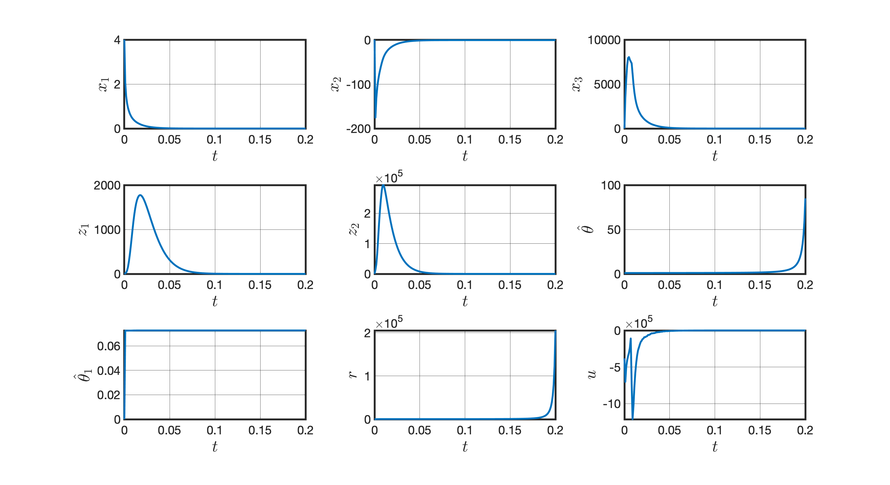
Figure 1: Simulations for closed-loop system (system (52) in closed loop with the prescribed-time stabilizing adaptive controller).

VI Conclusion

By combining a non-smooth control component ($u_{2}$ which involves the sign of $\eta^{T}P_{c}B$), time-dependent forcing functions in the definitions of both $u_{1}$ and $u_{2}$, an adaptation dynamics that incorporates temporal forcing terms, a time scale transformation $t\rightarrow\tau$, and dynamic scaling-based control design, it was shown that a prescribed-time stabilizing controller can be designed for a general class of nonlinear uncertain systems. The class of nonlinear systems considered allows several types of uncertainties including uncertain input gain and appended dynamics that effectively generate non-vanishing disturbances as well as a general structure of state-dependent uncertain terms throughout the system dynamics. While the adaptation parameter $\hat{\theta}$ and the dynamic scaling parameter $r$ grow (at most polynomially) as a function of the transformed time variable $\tau$, it was shown that the system state and input remain uniformly bounded and the system state $x$ converges to 0 in the prescribed time irrespective of the initial conditions of the system. Determining if similar control design approaches can be applied to other and more general classes of systems such as general cascade structures and non-triangular and feedforward systems as well as systems with unknown sign of the control gain remain topics for further research.

References

- [1] M. Krstić, I. Kanellakopoulos, and P. V. Kokotović, Nonlinear and Adaptive Control Design. New York: Wiley, 1995.
- [2] S. Jain and F. Khorrami, “Robust adaptive control of a class of nonlinear systems: state and output feedback,” in Proc. of the American Control Conf., Seattle, WA, June 1995, pp. 1580–1584.
- [3] A. Isidori, Nonlinear Control Systems II. London: Springer, 1999.
- [4] H. Khalil, Nonlinear Systems. Upper Saddle River, NJ: Prentice Hall, 2001.
- [5] V. Haimo, “Finite time controllers,” SIAM Journal on Control and Optimization, vol. 24, no. 4, pp. 760–770, 1986.
- [6] S. P. Bhat and D. S. Bernstein, “Finite-time stability of continuous autonomous systems,” SIAM Journal on Control and Optimization, vol. 38, no. 3, pp. 751–766, 2000.
- [7] X. Huang, W. Lin, and B. Yang, “Global finite-time stabilization of a class of uncertain nonlinear systems,” Automatica, vol. 41, no. 5, pp. 881–888, May 2005.
- [8] Y. Hong and Z. P. Jiang, “Finite-time stabilization of nonlinear systems with parametric and dynamic uncertainties,” IEEE Trans. on Automatic Control, vol. 51, no. 12, pp. 1950–1956, Dec. 2006.
- [9] S. Seo, H. Shim, and J. H. Seo, “Global finite-time stabilization of a nonlinear system using dynamic exponent scaling,” in Proc. of the IEEE Conf. on Decision and Control, Cancun, Mexico, Dec. 2008, p. 3805–3810.
- [10] E. Moulay and W. Perruquetti, “Finite time stability conditions for non-autonomous continuous systems,” Intl. Journal of Control, vol. 81, pp. 797–803, 2008.
- [11] Y. Shen and Y. Huang, “Global finite-time stabilisation for a class of nonlinear systems,” Intl. Journal of Systems Science, vol. 43, no. 1, pp. 73–78, 2012.
- [12] A. Polyakov, D. Efimov, and W. Perruquetti, “Finite-time and fixed-time stabilization: Implicit Lyapunov function approach,” Automatica, vol. 51, no. 1, pp. 332–340, Jan. 2015.
- [13] Z. Y. Sun, L. R. Xue, and K. M. Zhang, “A new approach to finite-time adaptive stabilization of high-order uncertain nonlinear system,” Automatica, vol. 58, pp. 60–66, Aug. 2015.
- [14] Z.-Y. Sun, M.-M. Yun, and T. Li, “A new approach to fast global finite-time stabilization of high-order nonlinear system,” Automatica, vol. 81, pp. 455–463, July 2017.
- [15] V. Andrieu, L. Praly, and A. Astolfi, “Homogeneous approximation, recursive observer design, and output feedback,” SIAM Journal on Control and Optimization, vol. 47, no. 4, pp. 1814–1850, 2008.
- [16] A. Polyakov, “Nonlinear feedback design for fixed-time stabilization of linear control systems,” IEEE Trans. on Automatic Control, vol. 57, no. 8, pp. 2106–2110, Aug. 2012.
- [17] A. Polyakov, D. Efimov, and W. Perruquetti, “Robust stabilization of MIMO systems in finite/fixed time,” Intl. Journal of Robust and Nonlinear Control, vol. 26, no. 1, pp. 69–90, Jan. 2016.
- [18] K. Zimenko, A. Polyakov, D. Efimov, and W. Perruquetti, “Finite-time and fixed-time stabilization for integrator chain of arbitrary order,” in Proc. of the European Control Conf., Limassol, Cyprus, June 2018, pp. 1631–1635.
- [19] K. Zimenko, A. Polyakov, D. Efimov, and W. Perruquetti, “On simple scheme of finite/fixed-time control design,” Intl. Journal of Control, Aug. 2018.
- [20] R. Aldana-López, D. Gómez-Gutiérrez, E. Jiménez-Rodríguez, J. D. Sánchez-Torres, and M. Defoort, “Enhancing the settling time estimation of a class of fixed-time stable systems,” Intl. Journal of Robust and Nonlinear Control, vol. 29, no. 12, pp. 4135–4148, Aug. 2019.
- [21] Y. Song, Y. Wang, J. Holloway, and M. Krstic, “Time-varying feedback for finite-time robust regulation of normal-form nonlinear systems,” in Proc. of the IEEE Conf. on Decision and Control, Las Vegas, NV, Dec. 2016, pp. 3837–3842.
- [22] Y. Song, Y. Wang, J. Holloway, and M. Krstic, “Time-varying feedback for regulation of normal-form nonlinear systems in prescribed finite time,” Automatica, vol. 83, pp. 243–251, Sept. 2017.
- [23] E. Jiménez-Rodríguez, J. D. Sánchez-Torres, D. Gómez-Gutiérrez, and A. G. Loukianov, “Predefined-time stabilization of high order systems,” in Proc. of the American Control Conf., Seattle, WA, May 2017, pp. 5836–5841.
- [24] E. Jiménez-Rodríguez, J. D. Sánchez-Torres, and A. G. Loukianov, “On optimal predefined-time stabilization,” Intl. Journal of Robust and Nonlinear Control, vol. 27, no. 17, pp. 3620–3642, Nov. 2017.
- [25] D. Tran, T. Yucelen, and B. Sarsilmaz, “Control of multiagent networks as systems: Finite-time algorithms, time transformation, and separation principle,” in Proc. of the IEEE Conf. on Decision and Control, Miami Beach, FL, Dec. 2018, pp. 6204–6209.
- [26] H. M. Becerra, C. R. Vázquez, G. Arechavaleta, and J. Delfin, “Predefined-time convergence control for high-order integrator systems using time base generators,” IEEE Trans. on Control Systems Technology, vol. 26, no. 5, pp. 1866–1873, Sept. 2018.
- [27] J. D. Sánchez-Torres, D. Gómez-Gutiérrez, E. López, and A. G. Loukianov, “A class of predefined-time stable dynamical systems,” IMA Journal of Mathematical Control and Information, vol. 35, no. Supplement 1, pp. i1–i29, April 2018.
- [28] Y. Song, Y. Wang, and M. Krstic, “Time-varying feedback for stabilization in prescribed finite time,” Intl. Journal of Robust and Nonlinear Control, vol. 29, no. 3, pp. 618–633, Feb. 2019.
- [29] J. D. Sánchez-Torres, M. Defoort, and A. J. Muñoz-Vázquez, “Predefined-time stabilisation of a class of nonholonomic systems,” Intl. Journal of Control, Jan. 2019.
- [30] K. Zhao, Y. Song, and Y. Wang, “Regular error feedback based adaptive practical prescribed time tracking control of normal-form nonaffine systems,” Journal of the Franklin Institute, vol. 356, no. 5, pp. 2759 – 2779, Mar. 2019.
- [31] P. Krishnamurthy, F. Khorrami, and M. Krstic, “Prescribed-time stabilization of nonlinear strict-feedback-like systems,” in Proc. of the American Control Conf., Philadelphia, PA, July 2019, pp. 3081–3086.
- [32] P. Krishnamurthy, F. Khorrami, and M. Krstic, “Robust output-feedback prescribed-time stabilization of a class of nonlinear strict-feedback-like systems,” in Proc. of the European Control Conf., Naples, Italy, June 2019, pp. 1148–1153.
- [33] P. Krishnamurthy, F. Khorrami, and M. Krstic, “Adaptive output-feedback prescribed-time stabilization of uncertain nonlinear strict-feedback-like systems,” in Proc. of the IEEE Conf. on Decision and Control, Nice, France, Dec. 2019.
- [34] P. Krishnamurthy and F. Khorrami, “Prescribed-time stabilization of nonlinear systems with uncertain input gain and non-vanishing disturbances,” in Proc. of the European Control Conference, Saint Petersburg, Russia, 2020, pp. 1859–1864.
- [35] P. Krishnamurthy and F. Khorrami, “Prescribed-time output-feedback stabilization of uncertain nonlinear systems with unknown time delays,” in Proc. of the American Control Conference, Denver, CO, USA, 2020, pp. 2705–2710.
- [36] P. Krishnamurthy and F. Khorrami, “Dynamic high-gain scaling: state and output feedback with application to systems with ISS appended dynamics driven by all states,” IEEE Trans. on Automatic Control, vol. 49, no. 12, pp. 2219–2239, Dec. 2004.
- [37] P. Krishnamurthy and F. Khorrami, “A high-gain scaling technique for adaptive output feedback control of feedforward systems,” IEEE Trans. on Automatic Control, vol. 49, no. 12, pp. 2286–2292, Dec. 2004.
- [38] P. Krishnamurthy and F. Khorrami, “Feedforward systems with ISS appended dynamics: Adaptive output-feedback stabilization and disturbance attenuation,” IEEE Trans. on Automatic Control, vol. 53, no. 1, pp. 405–412, Feb. 2008.
- [39] P. Krishnamurthy and F. Khorrami, “High-gain output-feedback control for nonlinear systems based on multiple time scaling,” Systems and Control Letters, vol. 56, no. 1, pp. 7–15, Jan. 2007.
- [40] P. Krishnamurthy and F. Khorrami, “Generalized state scaling and applications to feedback, feedforward, and non-triangular nonlinear systems,” IEEE Trans. on Automatic Control, vol. 52, no. 1, pp. 102–108, Jan. 2007.
- [41] P. Krishnamurthy and F. Khorrami, “Dual high-gain-based adaptive output-feedback control for a class of nonlinear systems,” Intl. Journal of Adaptive Control and Signal Processing, vol. 22, no. 1, pp. 23–42, Feb. 2008.
- [42] P. Krishnamurthy and F. Khorrami, “A singular perturbation based global dynamic high gain scaling control design for systems with nonlinear input uncertainties,” IEEE Trans. on Automatic Control, vol. 58, no. 10, pp. 2686–2692, Oct 2013.
- [43] P. Krishnamurthy and F. Khorrami, “A general dynamic scaling based control redesign to handle input unmodeled dynamics in uncertain nonlinear systems,” IEEE Trans. on Automatic Control, vol. 62, no. 9, pp. 4719–4726, Sep. 2017.
- [44] P. Krishnamurthy and F. Khorrami, “On uniform solvability of parameter-dependent Lyapunov inequalities and applications to various problems,” SIAM Journal of Control and Optimization, vol. 45, no. 4, pp. 1147–1164, 2006.
- [45] P. Krishnamurthy and F. Khorrami, “Conditions for uniform solvability of parameter-dependent Lyapunov equations with applications,” in Proc. of the American Control Conf., Boston, MA, July 2004, pp. 3896–3901.