Soliton resolution and asymptotic stability of $N$-soliton solutions for the defocusing mKdV equation with finite density type initial data

Abstract

We consider the Cauchy problem for the defocusing modified Korteweg-de Vries (mKdV) equation with finite density type initial data. With the $\bar{\partial}$ generalization of the nonlinear steepest descent method of Deift and Zhou, we extrapolate the leading order approximation to the solution of mKdV for large time in the solitonic space-time region $|x/t+4|<2$, and we give bounds for the error which decay as $t\rightarrow\infty$ for a general class of initial data whose difference from the non-vanishing background possesses a fixed number of finite moments. Our results provide a verification of the soliton resolution conjecture and asymptotic stability of $N$-soliton solutions for mKdV equation with finite density type initial data.
Keywords: The defocusing mKdV equation, Riemann-Hilbert problem, $\overline{\partial}$ steepest descent method, long-time asymptotics, asymptotic stability, soliton resolution.
Mathematics Subject Classification: 35Q51; 35Q15; 35C20; 37K15; 37K40.

1 Introduction

We investigate the Cauchy problem for the defocusing modified Korteweg-de Vries (mKdV) equation with finite density initial data

$$q_{t}+q_{xxx}-6q^{2}q_{x}=0,\hskip 14.22636pt(x,t)\in\mathbb{R}\times\mathbb{R}^{+},$$ (1.1)

$$q(x,0)=q_{0}(x)\rightarrow\pm 1,\hskip 14.22636ptx\rightarrow\pm\infty.$$ (1.2)

The mKdV equation arises in various of physical fields, such as acoustic wave and phonons in a certain anharmonic lattice [1, 2], Alfén wave in a cold collision-free plasma [3], meandering ocean currents [4], hyperbolic surfaces [5], and Schottky barrier transmission [6].

There is much work on the study of various mathematical properties for the mKdV equation. Here we cite only those that are closed to our consideration. In the early 1980s, the inverse scattering theory was applied to solve the mKdV equation and investigate long time asymptotics for the mKdV equation. For example, Wadati investigated the focusing mKdV equation with zero boundary conditions and derived simple-pole, double-pole and triple-pole solutions [7, 8]. Recently Zhang and Yan has studied the $N$-soliton solutions for focusing and defocusing mKdV equations with nonzero boundary conditions [9]. Segur and Ablowitz investigated the long-time behavior of solutions of the defocusing mKdV with given Schwartz initial data without consideration of solitons [10]. Deift and Zhou developed nonlinear steepest descent method and obtained the long-time asymptotic behavior of the defocusing mKdV equation with the Schwartz initial data [11]. This approach was further developed into a $\bar{\partial}$ steepest descent method by McLaughlin and Miller to analyze asymptotic of orthogonal polynomials with non-analytical weights [12, 13]. Later Dieng and McLaughin used it to study the defocusing NLS equation under essentially minimal regularity assumptions on finite mass initial data [14]. Boutet de Monvel et al. studied the initial boundary value problem of defocusing mKdV equation on the half line by using the Fokas method [15]. For the weighted Sobolev initial data, Chen and Liu et al. has studied the long-time asymptotic behavior of defocusing mKdV equation with zero boundary conditions without consideration of solitons [16]. However, for defocusing mKdV equations with nonzero boundary conditions, soliton solutions will appear due to empty discrete spectrum for finite mass initial data. It is necessary to consider affect of soliton solutions when we study long time asymptotic behavior, which naturally require a more detailed necessary description to obtain the long-time asymptotics of the defocusing mKdV equation.

Our goal in this paper is to give detailed asymptotic analysis for the defocusing mKdV equation (1.1) with finite density type initial data in different space-time solitonic regions. We investigate the asymptotic stability and soliton resolution for the mKdV equation (1.1) for the region $|x/t+4|<2$, in which there are no phase points on the real axis. For the case $|x/t+4|>2$, we will consider in our subsequent paper [24]. The soliton resolution conjecture is one of the most interesting phenomenon observed for solutions of nonlinear dispersive PDEs. It is widely believed that for many dispersive equations, solutions with generic initial data should eventually resolve into a finite number of solitons, moving at different speeds, plus a radiative term. For most dispersive evolution equations this is a wide open and active area of research [17, 18, 19]. The situation is somewhat better understood in the integrable system where the inverse scattering transform gives one much stronger control on the behavior of solutions than purely analytic techniques [20, 21, 22].

This paper is organized as follows. In Section 2, we get down to the spectral analysis on the Lax pair. For initial data $q_{0}(x)\pm 1\in L^{1,1}(\mathbb{R})$, the analyticity, symmetries and asymptotics of the Jost functions were discussed by Zhang and Yan [9]. However in our paper, to ensure reflection coefficient $r(z)\in H^{1}(\mathbb{R})$, we need $q_{0}(x)\pm 1\in H^{4,4}(\mathbb{R})$ and further show much strong properties for Jost functions and scattering data such as differentiability and Lipschitz continuity. In Section 3, we investigate the symmetries and asymptotic behaviors of the scattering data. For initial data $q_{0}(x)\pm 1\in H^{4,4}(\mathbb{R})$, we show that the reflection coefficient $r(z)\in H^{1}(\mathbb{R})$, which satisfies the additional estimates for sequential studies. It is shown that the zeros of $a(z)$ are simple and finite. In Section 4, we set up a Riemann-Hilbert (RH) problem for a sectionally meromorphic function $m(z)$ comprised by the Jost solutions and the scattering data. The reconstruction formula between $m(z)$ and the potential $q(x,t)$ of the mKdV equation (1.1) is further given. In Section 5, we use the $\bar{\partial}$ generalization of Deift-Zhou steepest descent procedure to get the long-time asymptotic of the mKdV equation (1.1) by a series of transformation. In section 5.1, we give the distributions of phase points and the signature table of $\operatorname*{Re}(2it\theta)$. In section 5.2, we introduce a set of conjugations and interpolations transformation, such that $m^{(1)}(z)$ becomes a standard RH problem. In section 5.3, according to the factorization of the jump matrix of the RH problem on the real line, we introduce some appropriate extensions to deform the jumps onto contours in the plane on which they are asymptotically small. While $\bar{\partial}$ derivatives satisfy particular bounds. In section 5.4, by ignoring the $\bar{\partial}$-component of $m^{(2)}(z)$, we get a conjugation of the RH problem corresponding to the $N$-soliton modified scattering data. In section 5.5, we consider the asymptotic behavior of $N$-soliton solutions by using a small norm theorem. In Section 5.6, we prove the existence of $m^{(3)}(z)$ and its asymptotic estimate its size according to the bounds on the $\bar{\partial}$-derivatives. Finally, in Section 6, summing up the estimates yields the proof of the main theorems.

2 Spectral analysis on the Lax pair

We denote $\mathbb{C}^{\pm}=\{z\in\mathbb{C}:\pm\operatorname*{Im}z>0\}$ and $\mathbb{R}^{+}=(0,\infty)$, and introduce the Japanese bracket $\langle x\rangle\doteq\sqrt{1+|x|^{2}}$. The normal spaces $L^{p,s}(\mathbb{R})$ is defined with $\|q\|_{L^{p,s}(\mathbb{R})}\doteq\|\langle x\rangle^{s}q\|_{L^{p,s}(\mathbb{R})}$; $W^{k,p}(\mathbb{R})$ is defined with $\|q\|_{W^{k,p}(\mathbb{R})}\doteq\sum_{j=0}^{k}\|\partial^{j}q\|_{L^{p}(\mathbb{R})}$; $H^{k}(\mathbb{R})$ is defined with $\|q\|_{H^{k}(\mathbb{R})}\doteq\|\langle x\rangle^{k}\hat{q}\|_{L^{2}(\mathbb{R})}$, where $\hat{u}$ is the Fourier transform of $u$, and $H^{k,k}(\mathbb{R})\doteq L^{2,k}(\mathbb{R})\cap H^{k}(\mathbb{R})$.

The defocusing mKdV equation (1.1) admits the following Lax pair

$$\frac{\partial\psi}{\partial x}=X\psi,\hskip 14.22636pt\frac{\partial\phi}{\partial t}=T\psi,$$ (2.1)

where $\psi=\psi(x,t;\lambda)$ is a matrix eigenfunction, $\lambda\in\mathbb{C}$ is the spectra parameter, and

$$X=X(x,t;\lambda)=i\lambda\sigma_{3}+Q;$$

$$T=T(x,t;\lambda)=4\lambda^{2}X-2i\lambda(z)\sigma_{3}(Q_{x}-Q^{2})+2Q^{3}-Q_{xx},$$

$$\sigma_{1}=\left(\begin{array}[]{cc}0&1\\ 1&0\\ \end{array}\right),\hskip 14.22636pt\sigma_{2}=\left(\begin{array}[]{cc}0&-i\\ i&0\\ \end{array}\right),\hskip 14.22636pt\sigma_{3}=\left(\begin{array}[]{cc}1&0\\ 0&-1\\ \end{array}\right).$$ (2.8)

$$Q(x,t)=\left(\begin{array}[]{cc}0&q(x,t)\\ q(x,t)&0\\ \end{array}\right).$$ (2.11)

Taking $q(x,t)=\pm 1$ in the Lax pair (2.1), we get the spectral problems

$$\frac{\partial\phi^{\pm}}{\partial x}=X_{\pm}\phi^{\pm},\hskip 14.22636pt\frac{\partial\phi^{\pm}}{\partial t}=T_{\pm}\phi^{\pm},$$ (2.12)

with

$$X_{\pm}(x,t;z)=i\lambda\sigma_{3}+Q_{\pm},\hskip 14.22636ptT_{\pm}(x,t;z)=(4\lambda^{2}+2)X_{\pm},\ \ \ Q_{\pm}=\pm\sigma_{1}.$$

The spectral problems (2.12) have a solution

$$\phi^{\pm}(z;x,t)=Y_{\pm}e^{it\theta(z;x,t)\sigma_{3}},$$ (2.13)

where

$$Y_{\pm}=I\mp\frac{1}{z}\sigma_{2},\hskip 14.22636pt\det Y_{\pm}=1-\frac{1}{z^{2}},$$

$$\theta(z;x,t)=\zeta(z)\left[\frac{x}{t}+4\lambda(z)^{2}+2\right],$$ (2.14)

and $\lambda$ and $\zeta$ are functions of uniformization variable $z$

$$\lambda=\frac{1}{2}(z+\frac{1}{z}),\hskip 14.22636pt\zeta=\frac{1}{2}(z-\frac{1}{z}).$$

We define the Jost solutions of Lax pair (2.1) with the following asymptotics

$$\psi^{\pm}(z;x,t)\sim\phi^{\pm}(z;x,t),\ \ x\rightarrow\pm\infty,$$

and making transformation

$$\mu^{\pm}(z;x,t)=\psi^{\pm}(z;x,t)e^{-it\theta(z;x,t)\sigma_{3}},$$

then $\mu^{\pm}(z;x,t)$ satisfy the Volterra integral equation

$$\mu^{\pm}(z;x,t)=\left\{\begin{aligned} &Y_{\pm}(z)+\int_{\pm\infty}^{x}Y_{\pm}(z)e^{i\zeta(z)(x-y)\hat{\sigma}_{3}}\big{[}Y_{\pm}^{-1}(z)\Delta Q_{\pm}(y,t)\mu_{\pm}(z;y,t)\big{]}dy,&&{z\neq\pm 1,}\\ &Y_{\pm}(z)+\int_{\pm\infty}^{x}\big{[}I+(x-y)(Q_{\pm}\pm i\sigma_{3})\big{]}\Delta Q_{\pm}(y,t)\mu_{\pm}(z;y,t)dy,&&{z=\pm 1,}\end{aligned}\right.$$

where $\Delta Q_{\pm}=Q-Q_{\pm}$.

Define $\mu_{1}^{\pm}(z;x,t)$ and $\mu_{2}^{\pm}(z;x,t)$ as the $1^{st}$ and $2^{nd}$ column of $\mu^{\pm}(z;x,t)$. Below we just take a quick review on the some propositions for the Jost functions $\mu_{1}^{\pm}(z;x,t)$, which can be shown in similar way to the reference [23].

Proposition 2.1.

Given $n\in\mathbb{N}_{0}$, let $q\mp 1\in$ $L^{1,n+1}(\mathbb{R})$, $q^{\prime}\in$ $W^{1,1}(\mathbb{R})$.

• For $z\in\mathbb{C}\setminus\{0\}$, $\mu_{1}^{+}(z;x,t)$ and $\mu_{2}^{-}(z;x,t)$ can be analytically extended to $\mathbb{C}^{+}$ and continuously extended to $\mathbb{C}^{+}\cup\Sigma$; $\mu_{1}^{-}(z;x,t)$ and $\mu_{2}^{+}(z;x,t)$ can be analytically extended to $\mathbb{C}^{-}$ and continuously extended to $\mathbb{C}^{-}\cup\Sigma$.

• The map $q\rightarrow$ $\frac{\partial^{n}}{\partial z^{n}}\mu^{\pm}_{i}(z)$ $(i=1,2,n\geq 0)$ are Lipschitz continuous, specifically, for any $x_{0}\in\mathbb{R}$, $\mu_{1}^{-}(z)$ and $\mu_{2}^{+}(z)$ are continuously differentiable mappings:

  $$\partial_{z}^{n}\mu_{1}^{-}:\bar{\mathbb{C}}^{-}\setminus\{0\}\rightarrow L^{\infty}_{loc}\{\bar{\mathbb{C}}^{-}\setminus\{0\},C^{1}((-\infty,x_{0}],\mathbb{C}^{2})\cap W^{1,\infty}((-\infty,x_{0}],\mathbb{C}^{2})\},$$ (2.15)

  $$\partial_{z}^{n}\mu_{2}^{+}:\bar{\mathbb{C}}^{-}\setminus\{0\}\rightarrow L^{\infty}_{loc}\{\bar{\mathbb{C}}^{-}\setminus\{0\},C^{1}([x_{0},\infty),\mathbb{C}^{2})\cap W^{1,\infty}([x_{0},\infty),\mathbb{C}^{2})\},$$ (2.16)

  $\mu_{1}^{+}(z)$ and $\mu_{2}^{-}(z)$ are continuously differentiable mappings:

  $$\partial_{z}^{n}\mu_{1}^{+}:\bar{\mathbb{C}}^{+}\setminus\{0\}\rightarrow L^{\infty}_{loc}\{\bar{\mathbb{C}}^{+}\setminus\{0\},C^{1}([x_{0},\infty),\mathbb{C}^{2})\cap W^{1,\infty}([x_{0},\infty),\mathbb{C}^{2})\},$$ (2.17)

  $$\partial_{z}^{n}\mu_{2}^{+}:\bar{\mathbb{C}}^{+}\setminus\{0\}\rightarrow L^{\infty}_{loc}\{\bar{\mathbb{C}}^{+}\setminus\{0\},C^{1}((-\infty,x_{0}],\mathbb{C}^{2})\cap W^{1,\infty}((-\infty,x_{0}],\mathbb{C}^{2})\}.$$ (2.18)

• Let $K$ be a compact neighborhood of $\{-1,1\}$ in $\bar{\mathbb{C}}^{+}\setminus\{0\}$. Set $x^{\pm}=\max\{\pm x,0\}$, then there exists a $C$ such that for $z\in K$ we have

  $$|\mu_{1}^{+}(z)-(1,z^{-1})^{T}|\leq C\langle x^{-}\rangle e^{C\int_{x}^{\infty}\langle y-x\rangle|q-1|dy}\|q-\tilde{q}\|_{L^{1,1}}(x,\infty),$$ (2.19)

  i.e., the map $z\rightarrow\mu_{1}^{+}(z)$ extends as a continuous map to the points $\pm 1$ with values in $C^{1}([x_{0},\infty),\mathbb{C})\cap W^{1,n}([x_{0},\infty),\mathbb{C})$ for any preassigned $x_{0}\in\mathbb{R}$. Moreover, the map $q\rightarrow\mu_{1}^{+}(z)$ is locally Lipschitz continuous from:

  $$L^{1,1}(\mathbb{R})\rightarrow L^{\infty}(\bar{\mathbb{C}}^{+}\setminus\{0\},C^{1}([x_{0},\infty),\mathbb{C})\cap W^{1,\infty}([x_{0},\infty),\mathbb{C}).$$ (2.20)

  Analogous statements hold for $\mu_{2}^{+}$ and for $\mu_{j}^{-}$ $(j=1,2)$. Furthermore, the maps $z\rightarrow\partial_{z}^{n}\mu_{1}^{+}(z)$ and $q\rightarrow\partial_{z}^{n}\mu_{1}^{+}(z)$ also satisfy:

  $$|\partial_{z}^{n}\mu_{1}^{+}(z)|\leq F_{n}[(1+|x|)^{n+1}\|q-1\|_{L^{1,n+1}(x,\infty)}],\hskip 14.22636ptz\in K.$$ (2.21)

The following proposition gives the asymptotic of the Jost solutions.

Proposition 2.2.

Suppose that $q\mp 1\in$ $L^{1,n+1}(\mathbb{R})$ and $q^{\prime}\in$ $W^{1,1}(\mathbb{R})$. Then as $z\rightarrow\infty$, with $\operatorname*{Im}z\geq 0$ we have

$$\mu_{1}^{+}(z)=e_{1}+\frac{1}{z}\left(\begin{array}[]{c}-i\int_{x}^{\infty}(q^{2}-1)dx\\ -iq\end{array}\right)+\mathcal{O}(z^{-2}),$$ (2.24)

$$\mu_{2}^{-}(z)=e_{2}+\frac{1}{z}\left(\begin{array}[]{c}iq\\ i\int_{x}^{\infty}(q^{2}-1)dx\end{array}\right)+\mathcal{O}(z^{-2}),$$ (2.27)

and for $\operatorname*{Im}z\leq 0$ as $z\rightarrow\infty$ we have

$$\mu_{1}^{-}(z)=e_{1}+\frac{1}{z}\left(\begin{array}[]{c}-i\int_{x}^{\infty}(q^{2}-1)dx\\ -iq\end{array}\right)+\mathcal{O}(z^{-2}),$$ (2.30)

$$\mu_{2}^{+}(z)=e_{2}+\frac{1}{z}\left(\begin{array}[]{c}iq\\ i\int_{x}^{\infty}(q^{2}-1)dx\end{array}\right)+\mathcal{O}(z^{-2}),$$ (2.33)

For $z\in\mathbb{C}^{+}$, as $z\rightarrow 0$, we have

$$\mu_{1}^{+}(z)=-\frac{i}{z}e_{2}+\mathcal{O}(1),\hskip 14.22636pt\mu_{2}^{-}(z)=-\frac{i}{z}e_{1}+\mathcal{O}(1);$$ (2.34)

for $z\in\mathbb{C}^{-}$, as $z\rightarrow 0$, we have

$$\mu_{1}^{-}(z)=\frac{i}{z}e_{2}+\mathcal{O}(1),\hskip 14.22636pt\mu_{2}^{+}(z)=\frac{i}{z}e_{1}+\mathcal{O}(1);$$ (2.35)

Proposition 2.3.

Let $q\mp 1\in$ $L^{1,n+1}(\mathbb{R})$ and $q^{\prime}\in$ $W^{1,1}(\mathbb{R})$, then

1. For $z\in\mathbb{C}\setminus\{0\}$, both of the matrix-valued functions

   $$\psi^{\pm}(z)=(\psi_{1}^{\pm}(z),\psi_{2}^{\pm}(z))=(\mu_{1}^{\pm}(z),\mu_{2}^{\pm}(z))e^{it\theta(z;x)\sigma_{3}}$$ (2.36)

   are singular solutions of (2.1) and

   $$\det\psi^{\pm}(z)=1-z^{-2}.$$ (2.37)

2. For $z\in\bar{\mathbb{C}}^{+}\setminus\{0\}$, the Jost functions $\psi_{j}^{\pm}$ $(j=1,2)$ satisfy the symmetries

   $$\psi_{1}^{\pm}(z)=\sigma_{1}\overline{\psi_{2}^{\pm}(\bar{z})},\ \ \ \psi_{2}^{\pm}(z)=\sigma_{1}\overline{\psi_{1}^{\pm}(\bar{z})}.$$ (2.38)

   $$\psi_{1}^{\pm}(z)=\overline{\psi_{1}^{\pm}(-\bar{z})},\ \ \psi_{2}^{\pm}(z)=\overline{\psi_{2}^{\pm}(-\bar{z})}.$$ (2.39)

   $$\psi_{1}^{\pm}(z)=\mp\frac{i}{z}\psi_{2}^{\pm}(\frac{1}{z}),\ \ \ \psi_{2}^{\pm}(z)=\pm\frac{i}{z}\psi_{1}^{\pm}(\frac{1}{z}).$$ (2.40)

The columns of $\psi^{+}(z;x,t)$ and $\psi^{-}(z;x,t)$ satisfy the linear relation

$$\psi^{+}(z;x,t)=\psi^{-}(z;x,t)S(z),\hskip 14.22636ptS(z)=\left(\begin{array}[]{cc}a(z)&\overline{b(\bar{z})}\\ b(z)&\overline{a(\bar{z})}\end{array}\right),\hskip 14.22636ptz\in\mathbb{R}\setminus\{\pm 1,0\}$$ (2.41)

3 The Scattering map

We use the scattering coefficients $a(z)$ and $b(z)$ to define the reflection coefficient

$$r(z)\doteq\frac{b(z)}{a(z)}.$$ (3.1)

The following proposition provides some essential properties of $a(z)$ and $b(z)$.

Proposition 3.1.

Let $q\mp 1\in$ $L^{1,n+1}(\mathbb{R})$ and $q^{\prime}\in$ $W^{1,1}(\mathbb{R})$, then

1. The scattering coefficients can be expressed by the Jost functions as

   $$a(z)=\frac{\det[\psi_{1}^{+},\psi_{2}^{-}]}{1-z^{-2}},\hskip 14.22636ptb(z)=\frac{\det[\psi_{1}^{-},\psi_{1}^{+}]}{1-z^{-2}}$$ (3.2)

   Thus it can be seen that $a(z)$ extends analytically to $z\in\mathbb{C}^{+}$ while $b(z)$ and $r(z)$ are defined only for $z\in\mathbb{R}\setminus\{\pm 1,0\}$.

2. The scattering data satisfy the following symmetries:

   $$S(z)=\overline{S(-\bar{z})};\hskip 14.22636ptS(z)=-\sigma_{2}S(z^{-1})\sigma_{2}.$$ (3.3)

3. For each $z\in\mathbb{R}\setminus\{\pm 1,0\}$,

   $$|a(z)|^{2}-|b(z)|^{2}=1.$$ (3.4)

   In particular, for $z\in\mathbb{R}\setminus\{\pm 1,0\}$, we have

   $$|r(z)|^{2}=1-\frac{1}{|a(z)|^{2}}<1.$$ (3.5)

4. The scattering data have the asymptotics

   $$\lim_{z\rightarrow\infty}(a(z)-1)z=i\int_{\mathbb{R}}(q^{2}-1)dx,\ z\in\bar{\mathbb{C}}^{+},$$ (3.6)

   $$\lim_{z\rightarrow 0}(a(z)+1)z^{-1}=i\int_{\mathbb{R}}(q^{2}-1)dx,\ z\in\bar{\mathbb{C}}^{+}$$ (3.7)

   $$|b(z)|=\mathcal{O}(|z|^{-2}),\hskip 14.22636pt\text{as }|z|\rightarrow\infty,\ \ z\in\mathbb{R}$$ (3.8)

   $$|b(z)|=\mathcal{O}(|z|^{2}),\hskip 14.22636pt\text{as }|z|\rightarrow 0,\ z\in\mathbb{R}.$$ (3.9)

   So that

   $$r(z)\sim z^{-2},\hskip 5.69046pt|z|\rightarrow\infty;\hskip 14.22636ptr(z)\sim 0,\hskip 5.69046pt|z|\rightarrow 0.$$ (3.10)

Although Proposition 3.1 gives conditions on $q$ to ensure that the Jost functions $\psi_{j}^{\pm}$ are continuous for $z\rightarrow\pm 1$, these points are still the simple poles of the scattering coefficients $a(z)$ and $b(z)$ on account of the vanishing of denominators in (3.2). Meanwhile, their residues are proportional: the symmetry (2.40) demonstrates that $\psi_{1}^{-}(\pm 1)=\pm i\psi_{2}^{-}(\pm 1)$, which in turn gives

$$a(z)=\frac{\pm a_{\pm}}{z\mp 1}+\mathcal{O}(1),\hskip 14.22636ptb(z)=\frac{ia_{\pm}}{z\mp 1}+\mathcal{O}(1),$$ (3.11)

where

$$a_{\pm}=\frac{1}{2}\det[\psi_{1}^{+}(\pm 1),\psi_{2}^{-}(\pm 1)].$$

On this occasion, the reflection coefficient is still bounded at $z=\pm 1$ and we have

$$\lim_{z\rightarrow\pm 1}r(z)=\mp i.$$ (3.12)

The next lemma shows that, given data $q_{0}$ with sufficient smoothness and decay properties, the reflection coefficients will also be smooth and decaying.

Proposition 3.2.

For given $q\mp 1\in L^{1,2}(\mathbb{R})$, $q^{\prime}\in W^{1,1}(\mathbb{R})$, we then have $r(z)\in H^{1}(\mathbb{R})$.

Proof.

Proposition 2.1 and (3.2) indicate that $a(z)$ and $b(z)$ are continuous when $z\in\mathbb{R}\setminus\{\pm 1,0\}$. Then $r(z)$ is continuous when $z\in\mathbb{R}\setminus\{\pm 1,0\}$. From (3.10) and (3.12) we know that $r(z)$ is bounded in the small neighborhood of $\{\pm 1,0\}$ and $r(z)\in L^{1}(\mathbb{R})\cap L^{2}(\mathbb{R})$. Then we just need to prove that $r^{\prime}(z)\in L^{2}(\mathbb{R})$. For $\delta_{0}>0$ sufficiently small, from Proposition 2.1, the maps

$$q\rightarrow\det[\psi_{1}^{+}(z),\psi_{2}^{-}(z)]\hskip 14.22636pt\text{and}\hskip 14.22636ptq\rightarrow\det[\psi_{1}^{-}(z),\psi_{1}^{+}(z)]$$ (3.13)

are locally Lipschitz maps from

$$\{q:q^{\prime}\in W^{1,1}(\mathbb{R})\text{ and }q\in L^{1,n+1}(\mathbb{R})\}\rightarrow W^{n,\infty}(\mathbb{R}\setminus(-\delta_{0},\delta_{0}))\text{ for }n\geq 0.$$ (3.14)

Actually, $q\rightarrow\psi_{1}^{+}(z,0)$ is, by Proposition 2.1, a locally Lipschitz map with values in $W^{n,\infty}(\bar{\mathbb{C}}^{+}\setminus D(0,\delta_{0}),\mathbb{C}^{2})$. For $q\rightarrow\psi_{2}^{-}(z,0)$ and $q\rightarrow\psi_{1}^{-}(z,0)$ the same is true. These and (3.6)-(3.9) imply that $q\rightarrow r(z)$ is a locally Lipschitz map from the domain in (3.14) into

$$W^{n,\infty}(I_{\delta_{0}})\cap H^{n}(I_{\delta_{0}}),$$ (3.15)

where $I_{\delta_{0}}\doteq\mathbb{R}\setminus((-\delta_{0},\delta_{0})\cup(1-\delta_{0},1+\delta_{0})\cup(-1-\delta_{0},-1+\delta_{0})).$ Now fix $\delta_{0}>0$ sufficiently small such that the 3 intervals dist$(z,\{\pm 1\})\leq\delta_{0}$ and $|z|\leq\delta_{0}$ have no intersection. In the complement of their union

$$|\partial_{z}^{j}r(z)|\leq C_{\delta_{0}}\langle z\rangle^{-1}\text{ for }j=0,1,$$ (3.16)

it’s analogous for the other Jost functions, and the discussion above. In the following, we will just prove the boundedness of $r(z)$ in the small neighborhood of $z=1$.

Let $|z-1|<\delta_{0}$. Then using the definition of $a_{+}$ we have

$$r(z)=\frac{b(z)}{a(z)}=\frac{\det[\psi_{1}^{-},\psi_{1}^{+}]}{\det[\psi_{1}^{+},\psi_{2}^{-}]}=\frac{\int_{1}^{z}F(s)ds-2ia_{+}}{\int_{1}^{z}G(s)ds+2a_{+}},$$ (3.17)

where

$$F(s)=\partial_{s}\det[\psi_{1}^{-}(s),\psi_{1}^{+}(s)],\hskip 14.22636ptG(s)=\partial_{s}\det[\psi_{1}^{+}(s),\psi_{1}^{-}(s)].$$ (3.18)

If $a_{+}\neq 0$ then it is clear from the above formula that $r^{\prime}(z)$ exist and is bounded near $1$.

If $a_{+}=0$, then $z=1$ is not the pole of $a(z)$ and $b(z)$, so that $a(z)$ and $b(a)$ are continuous at $z=1$, then

$$r(z)=\frac{\int_{1}^{z}F(s)ds}{\int_{1}^{z}G(s)ds}.$$ (3.19)

From (3.2) we know that

$$(z^{2}-1)a(z)=z^{2}\det[\psi_{1}^{+},\psi_{2}^{-}].$$ (3.20)

While $a_{+}=0$ implies that $\det[\psi_{1}^{+},\psi_{2}^{-}]|_{z=1}=0$, differentiating (3.20) at $z=1$ we get

$$2a(1)=\partial_{z}\det[\psi_{1}^{+},\psi_{2}^{-}]|z=1=G(1).$$ (3.21)

With $|a(1)|^{2}=1+|b(1)|^{2}\geq 1$, we have $G(1)\neq 0$. It follows that the derivative $r^{\prime}(z)$ is bounded around $1$.

The same proof holds at $z=-1$. At $z=0$ we can use the symmetry $r(z^{-1})=-\bar{r}(z)$ to infer that $r(z)$ vanished. It follows that $r^{\prime}(z)\in L^{2}(\mathbb{R})$. ∎

Remark 3.1.

The smoothness and decay properties of the reflection coefficient required in the proof of the above theorem, which depend on the hypotheses on $q_{0}$, are proved in Sec.3. Explicitly, as $q_{0}\mp 1\in H^{k,k}$ with $k=2$ we have the result that $r\in L^{2}(\mathbb{R})$ and $\|\log(1-|r|^{2})\|_{L^{p}(\mathbb{R})}<\infty$ for $p\geq 1$; as $k=3$ we have $q_{0}\mp 1\in L^{1,2}(\mathbb{R})$ which in turn shows that $r(z)\in H^{1}(\mathbb{R})$ and we can also elicit that the quantity of the discrete spectrum is finite under this assumption; while $k=4$ is demanded only when we bound the $\bar{\partial}$ derivatives of the extensions of the reflection coefficient.

We also have the following proposition, whose proof can be found in [23].

Proposition 3.3.

For any initial data $q_{0}$ such that $q_{0}\mp 1\in H^{2,2}$ the reflection coefficient satisfies

$$\|\log(1-|r|^{2})\|_{L^{p}(\mathbb{R})}<\infty\text{ for any }p\geq 1.$$ (3.22)

Now we give the discrete spectrum. Suppose that $a(z)$ has finite $N$ simple zeros $z_{k},\ k=0,\cdots,N-1$ on $D_{1}\doteq\{z\in\mathbb{C}^{+}:\operatorname*{Im}z>0,\operatorname*{Re}z\geq 0\}$, then from the symmetries (3.3) we know that the discrete spectrum can be expressed as

$$\mathcal{Z}=\{z_{k},\bar{z}_{k},-\bar{z}_{k},-z_{k}\}_{k=0}^{N-1}.$$

When $z_{k}=-\bar{z}_{k}$, the corresponding four zeros $\{z_{k},\bar{z}_{k},-\bar{z}_{k},-z_{k}\}$ degenerate into two zeros $\{-i,i\}$, which corresponds to solitons. We further classify these discrete spectrum as

$$\mathcal{Z}_{1}=\{z_{k}\}_{k=0}^{N-1},\ \ \mathcal{Z}_{2}=\{-\bar{z}_{k}\}_{0}^{N-1},\ \ \mathcal{Z}^{+}\doteq\mathcal{Z}_{1}\cup\mathcal{Z}_{2},\ \ \mathcal{Z}=\mathcal{Z}^{+}\cup\overline{\mathcal{Z}^{+}},$$

where $\overline{\mathcal{Z}^{+}}$ formed by the complex conjugates of $\mathcal{Z}^{+}$. The discrete spectrum can be seen in Figure 1.

Figure 1: Distribution of the discrete spectrum: the jump contour $\mathbb{R}$, the red dots ($\centerdot$ ) and ($\centerdot$ ) represent the poles, they are correspond to breathers and solitons respectively. The blue dots ($\centerdot$) represent singularities.

In the following we will prove that the zeros of $a(z)$ are simple, finite and all distribute on the circle $|z|=1$. From the symmetries of $\psi^{\pm}(z)$ we know that there exists a constant $\gamma_{k}\in\mathbb{C}$ such that

$$\psi_{1}^{+}(z_{k})=\gamma_{k}\psi_{2}^{-}(z_{k}),\hskip 14.22636pt\psi_{2}^{+}(z_{k})=\bar{\gamma}_{k}\psi_{1}^{-}(z_{k}),\hskip 14.22636pt\psi_{1}^{+}(z_{k})=\gamma_{k}\psi_{2}^{-}(-\bar{z}_{k}),$$ (3.23)

where $\gamma_{k}$ is called the connection coefficient associated with the discrete spectral point $z_{k}$. We can further show that

Proposition 3.4.

Let $q\mp 1\in L^{1,2}(\mathbb{R})$. Then the zeros of $a(z)$ are simple and finite.

Proof.

First we prove that the zeros of $a(z)$ in $D_{1}$ are simple and finite.

From (2.1) we can get that $X$ is self-adjoint, so that $\lambda\in\mathbb{R}$. Then

$$\operatorname*{Im}\lambda=\frac{|z|^{2}-1}{2|z|^{2}}\operatorname*{Im}z=0,$$ (3.24)

from which we can obtain $|z|^{2}=1$ directly. So that all the zeros of $a(z)$ are distribute on the real axis and the unit circle. The functions

$$f_{k}^{\theta}=|\partial_{\theta}^{k}\det[\psi_{1}^{+}(e^{i\theta}),\psi_{2}^{-}(e^{i\theta})]|,\hskip 14.22636ptk=0,1$$ (3.25)

are continuous for $\theta\in[0,\pi/2]$. If $z=1$ is an accumulation points, according to the Bolzano-Weierstrass theorem, there exist sequences $\theta_{j}^{(k)}$, $k=0,1$, with $\lim_{j\rightarrow\infty}\theta_{j}^{(k)}=0$ and $f_{k}(\theta_{j}^{(k)})=0$ for each $j$. It then follows that $a(z)=o(1)$ as $z\rightarrow 1$. This contradicts the fact that $|a(z)|^{2}\geq 1$ for $z\in\mathbb{R}\setminus\{0,\pm 1\}$. The proof when $z=-1$ is an accumulation point is the same.

From the symmetries of $\Psi^{\pm}$, we have

$$\overline{\psi_{1}^{+}(\bar{z}_{k})^{-1}}=\bar{\gamma}_{k}\overline{\psi_{2}^{-}(\bar{z}_{k}^{-1})},\ \ \sigma_{1}\psi_{2}^{+}(z_{k}^{-1})=\bar{\gamma}_{k}\sigma_{1}\psi_{1}^{-}(z_{k}^{-1}),$$

$$\psi_{1}^{+}(z_{k})=\bar{\gamma}_{k}\psi_{2}^{-}(z_{k}),$$

which show that $\gamma_{k}=\bar{\gamma}_{k}$, this is to say, $\gamma_{k}\in\mathbb{R}$. Note that $q\mp 1\in L^{1,1}(\mathbb{R})$ implies $\frac{\partial a}{\partial\lambda}$ exists and we have from (3.2)

$$\frac{\partial a}{\partial\lambda}\mid_{z=z_{k}}={\frac{\det[\partial_{\lambda}\psi_{1}^{+},\psi_{2}^{-}]+\det[\psi_{1}^{+},\partial_{\lambda}\psi_{2}^{-}]}{1-z^{-2}}}\mid_{z=z_{k}}.$$ (3.26)

Using (2.1) we find that

$$\frac{\partial}{\partial x}\det[\partial_{\lambda}\psi_{1}^{+},\psi_{2}^{-}] =\det[X_{\lambda}\psi_{1}^{+},\psi_{2}^{-}]+\det[X\partial_{\lambda}\psi_{1}^{+},\psi_{2}^{-}]+\det[\partial_{\lambda}\psi_{1}^{+},X\psi_{2}^{-}]$$

$$=i\det[\sigma_{3}\psi_{1}^{+},\psi_{2}^{-}],$$

and

$$\frac{\partial}{\partial x}\det[\lambda\psi_{1}^{+},\partial\psi_{2}^{-}] =\det[\psi_{1}^{+},X_{\lambda}\psi_{2}^{-}]+\det[X\psi_{1}^{+},\partial_{\lambda}\psi_{2}^{-}]+\det[\psi_{1}^{+},X\partial_{\lambda}\psi_{2}^{-}]$$

$$=i\det[\psi_{1}^{+},\sigma_{3}\psi_{2}^{-}]$$

where the cancellation in each equality follows from adj$X=-X$. Recalling that at each $z_{k}$ the columns are linearly dependent according to (3.23) and decay exponentially as $|x|\rightarrow\infty$.

$$\det[\partial_{\lambda}\psi_{1}^{+},\psi_{2}^{-}]=i\gamma_{k}\int_{-\infty}^{x}\det[\sigma_{3}\psi_{2}^{-}(z_{k},s),\psi_{2}^{-}(z_{k},s)]ds,$$

$$\det[\psi_{1}^{+},\partial_{\lambda}\psi_{2}^{-}]=i\gamma_{k}\int_{x}^{\infty}\det[\sigma_{3}\psi_{2}^{-}(z_{k},s),\psi_{2}^{-}(z_{k},s)]ds$$

∎

The zeros of $a(z)$ are simple, finite and restricted to the unit circle. As $a(z)$ is analytic in $\mathbb{C}^{+}$, and approaches unity for large $z$. Then we have the trace formula

$$a(z)=\prod_{n=0}^{N-1}\frac{(z-z_{n})(z+\bar{z}_{n})}{(z-\bar{z}_{n})(z+z_{n})}\exp\left(-\frac{1}{2\pi i}\int_{\mathbb{R}}\frac{\log(1-|r(s)|^{2})}{s-z}ds\right),$$ (3.27)

where as $z_{n}=i$, the item $\frac{(z-z_{n})(z+\bar{z}_{n})}{(z-\bar{z}_{n})(z+z_{n})}$ degenerate to $\frac{z-i}{z+i}$.

4 Set up of the Riemann-Hilbert problem

For $z\in\mathbb{C}\setminus\mathbb{R}$, for $q(x,t)$ the solution of (1.1), and for $\mu_{j}^{\pm}(z;x,t)$ ($j=1,2$) the Jost functions we set

$$m(z)=m(z;x,t)=\left\{\begin{aligned} &\left(\frac{\mu_{1}^{+}(z;x,t)}{a(z)},\mu_{2}^{-}(z;x,t)\right),&&z\in\mathbb{C}^{+},\\ &\left(\mu_{1}^{-}(z;x,t),\frac{\mu_{2}^{+}(z;x,t)}{\overline{a(\bar{z})}}\right),&&z\in\mathbb{C}^{-}.\end{aligned}\right.$$ (4.1)

Proposition 4.1.

We have the following symmetries for $m(z)$

$$m(z)=\sigma_{1}\overline{m(\bar{z})}\sigma_{1},\ \ m(z)=\overline{m(-\bar{z})},\ \ m(z^{-1})=zm(z)\sigma_{2}.$$ (4.2)

Proposition 4.2.

Assume $q\mp 1\in L^{1,2}(\mathbb{R})$ and $q^{\prime}(x)\in W^{1,1}(\mathbb{R})$, we have the following asymptotics of $m(z)$ as $z\rightarrow\infty$ and $z\rightarrow 0$:

$$\lim_{z\rightarrow\infty}z(m(z)-I)=\left(\begin{array}[]{cc}-i\int_{x}^{\infty}(q^{2}-1)dx&iq\\ -iq&i\int_{x}^{\infty}(q^{2}-1)dx\end{array}\right),$$ (4.5)

$$\lim_{z\rightarrow 0}(m(z)-\frac{\sigma_{2}}{z})=\left(\begin{array}[]{cc}iq&-i\int_{x}^{\infty}(q^{2}-1)dx\\ i\int_{x}^{\infty}(q^{2}-1)dx&-iq\end{array}\right).$$ (4.8)

The above propositions indicate that $m(z;x,t)$ satisfies the following Riemann-Hilbert problem.

RHP 4.1.

Find a $2\times 2$ matrix valued function $m(z;x,t)$ such that

1. $m(z)$ is meromorphic for $z\in\mathbb{C}\setminus\mathbb{R}$.

2. $m(z)$ has the following asymptotics

   $$m(z;x,t)=I+\mathcal{O}(z^{-1}),\hskip 14.22636ptz\rightarrow\infty,$$

   $$zm(z;x,t)=\sigma_{2}+\mathcal{O}(z),\hskip 14.22636ptz\rightarrow 0.$$

3. The non-tangential limits $m_{\pm}(z;x,t)=\lim_{\mathbb{C}^{\pm}\ni z^{\prime}\rightarrow z}m(z^{\prime};x,t)$ exist for any $z\in\mathbb{R}\setminus\{0\}$ and satisfy the jump relation $m_{+}(z;x,t)=m_{-}(z;x,t)V(z)$

   $$V(z)=\left(\begin{array}[]{cc}1-|r(z)|^{2}&-\overline{r(z)}e^{2it\theta(z)}\\ r(z)e^{-2it\theta(z)}&1\end{array}\right)$$ (4.9)

   where $\theta(z)=\zeta(z)\{x/t+4\lambda^{2}(z)+2\}$.

4. $m(z;x,t)$ has simple poles at points $\mathcal{Z}=\mathcal{Z}^{+}\cup\overline{\mathcal{Z}^{+}}$ with residues satisfying

   $$\begin{split}\operatorname*{Res}_{z=z_{k}}m(z;x,t)=\lim_{z\rightarrow z_{k}}m(z;x,t)\left(\begin{array}[]{cc}0&0\\ c_{k}(x,t)&0\end{array}\right),\\ \operatorname*{Res}_{z=\bar{z}_{k}}m(z;x,t)=\lim_{z\rightarrow\bar{z}_{k}}m(z;x,t)\left(\begin{array}[]{cc}0&\bar{c}_{k}(x,t)\\ 0&0\end{array}\right),\\ \operatorname*{Res}_{z=-\bar{z}_{k}}m(z;x,t)=\lim_{z\rightarrow-\bar{z}_{k}}m(z;x,t)\left(\begin{array}[]{cc}0&0\\ -\bar{c}_{k}(x,t)&0\end{array}\right),\\ \operatorname*{Res}_{z=-z_{k}}m(z;x,t)=\lim_{z\rightarrow-z_{k}}m(z;x,t)\left(\begin{array}[]{cc}0&-c_{k}(x,t)\\ 0&0\end{array}\right),\end{split}$$ (4.10)

   where

   $$\begin{split}&c_{k}(x,t)=\frac{\gamma_{k}(0)}{a^{\prime}(z_{k})}e^{-2it\theta(z_{k})}\doteq c_{k}e^{-2it\theta(z_{k})},\\ &c_{k}=\frac{\gamma_{k}(0)}{a^{\prime}(z_{k})}=\frac{2z_{k}}{\int_{\mathbb{R}}|\psi_{2}^{+}(z_{k};x,0)|^{2}dx}=z_{k}|c_{k}|.\end{split}$$ (4.11)

The potential $q(x,t)$ is found by the reconstruction formula, see Proposition 4.1,

$$q(x,t)=\lim_{z\rightarrow\infty}izm_{21}(z;x,t).$$ (4.12)

While the $N$-solitons are potentials corresponding to the case when $r(z)\equiv 0$.

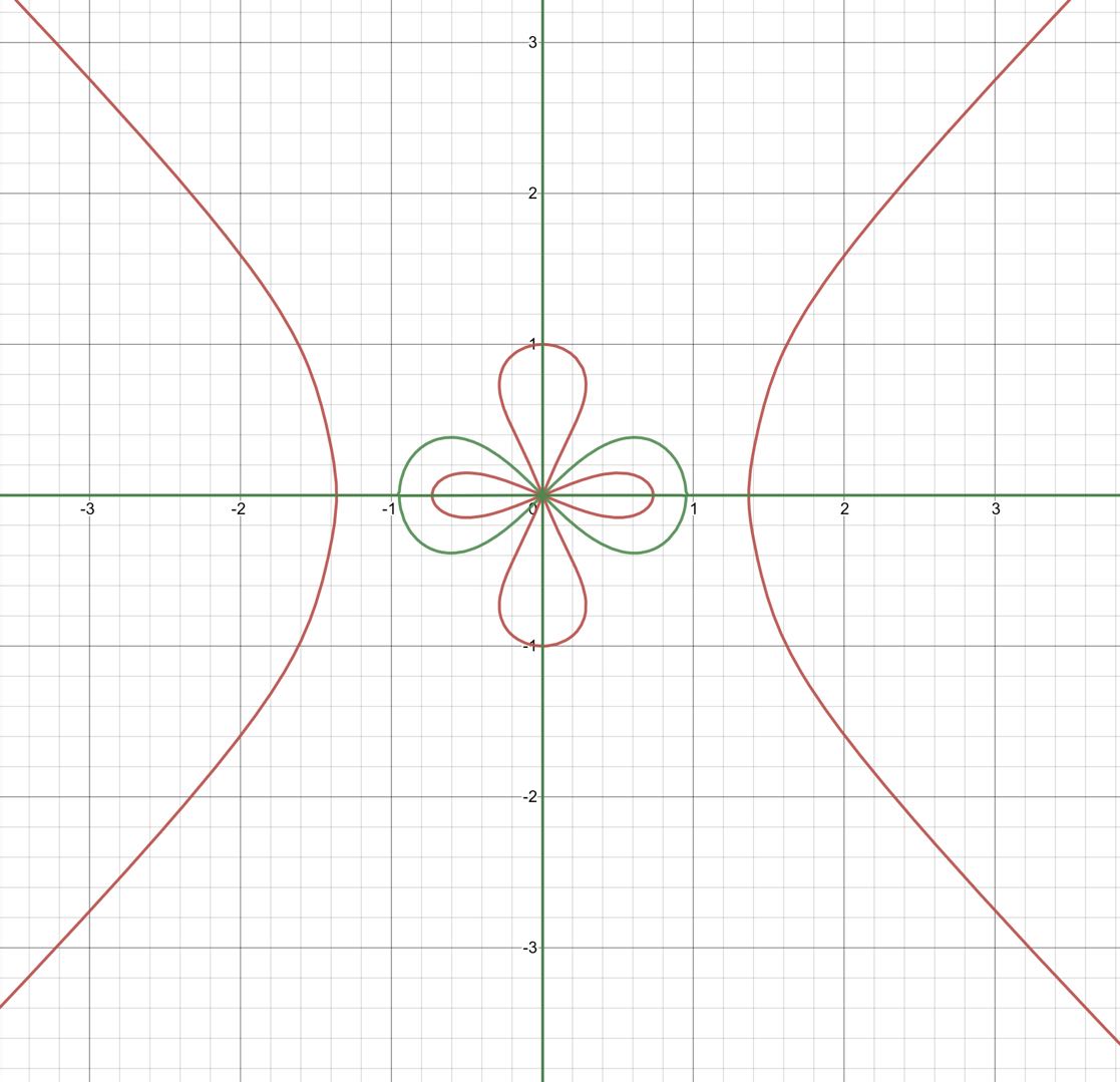
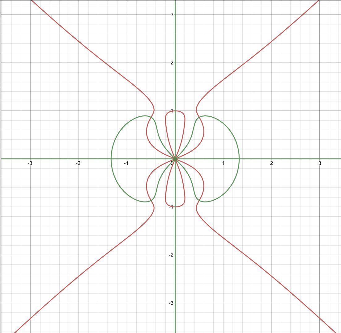
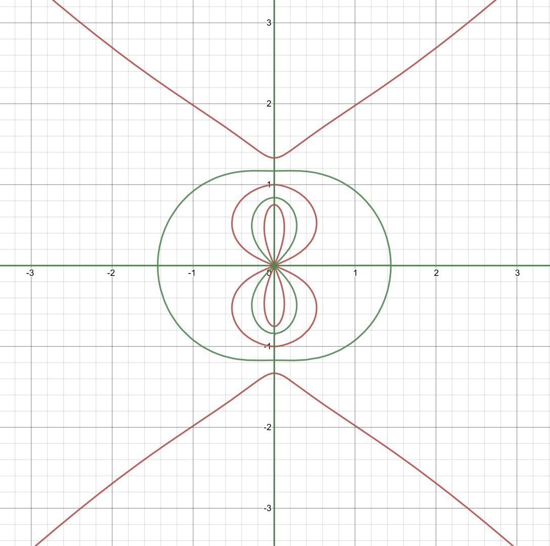
Figure 2: Plots of the distributions for phase points: (a) $\xi<-6$, (b) $-6<\xi<6$, (c) $\xi>-6$. The red curves show the ${\rm Re}\theta^{\prime}(z)=0$, and the green curves show the ${\rm Im}\theta^{\prime}(z)=0$. The intersection points are the saddle points which express $\theta^{\prime}(z)=0$.

5 The long time asymptotic analysis

In this section, we will give two important operations for the sake of using the $\bar{\partial}$ steepest method to do the long time analysis: Interpolate the poles through converting them to jumps with small closed loops enclosing each pole; The factorization of the jump matrix along the real axis is used to deform the contours onto those on which the oscillatory jump on the real axis convert to exponential decay.

5.1 Stationary phase points and decay domains

Long-time asymptotic behavior of RHP 4.1 is influenced by decay/growth of oscillatory terms $e^{\pm 2it\theta(z)}$ and phase points of $\theta(z)$. Let $\xi=x/t$, direct calculation gives

$$\theta^{\prime}(z)=\frac{3}{2}z^{2}+\frac{\xi+3}{2z^{2}}+\frac{3}{2z^{4}}+\frac{\xi+3}{2},$$

from which we can get six phase points. Except to $z=\pm i$, there are also four phase points, whose distribution is as follows.

• For the case $-6<\xi<-2$, there is no phase point on real axis $\mathbb{R}$ corresponding to Fig. 2, which will be discussed by by this paper;

• For the cases $\xi<-6$ and $\xi>-2$, four phase points are local on real axis $\mathbb{R}$ and imaginary axis $\mathbb{R}$ respectively corresponding to Fig. 2 and Fig. 2, which were discussed by our paper [24]. The distributions of stationary phase points are shown in Fig. 2.

The decay/growth of oscillatory terms $e^{\pm 2it\theta(z)}$ is determined by the sign of ${\rm Re}(2it\theta(z))$. The decaying regions of ${\rm Re}(2it\theta(z))$ are shown in Fig. 3.

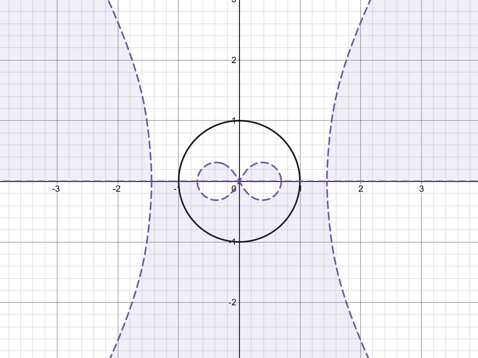
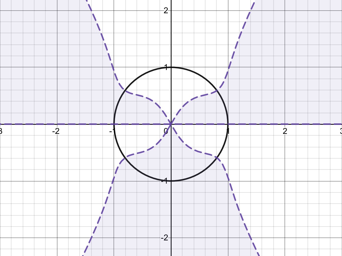
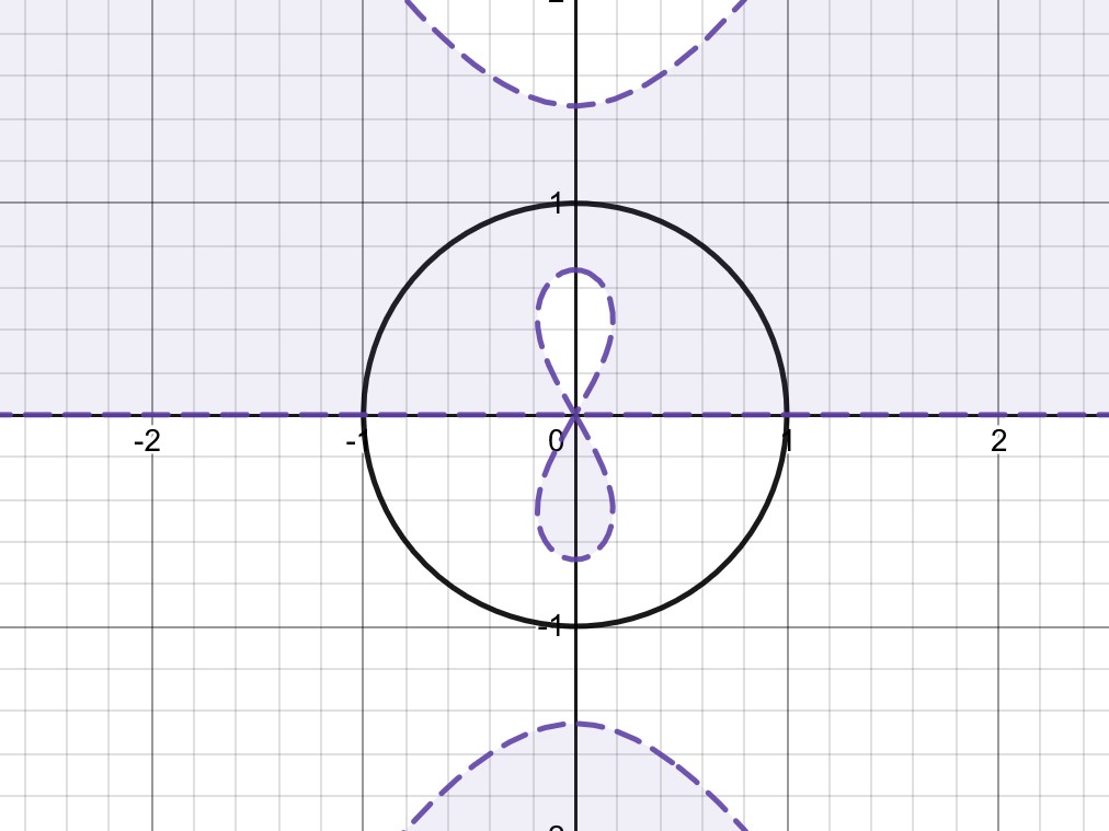
Figure 3: Signature table of ${\rm Re}(2it\theta(z))$ with different $\xi$: (a) $\xi<-6$, (b) $-6<\xi<-2$, (c) $\xi>-2$. In the purple region, $\operatorname*{Re}(2i\theta)<0$, while in the white region, $\operatorname*{Re}(2i\theta)>0$. The purple dotted lines are the critical lines.

5.2 Interpolation and conjugation

The second step is done by a well known factorization of the jump matrix $V(z)$

$$V(z)=\left(\begin{array}[]{cc}1-|r(z)|^{2}&-\overline{r(z)}e^{2it\theta(z)}\\ r(z)e^{-2it\theta(z)}&1\end{array}\right)=B(z)T_{0}(z)B(z)^{-{\dagger}},$$ (5.1)

where

$$B(z)=\left(\begin{array}[]{cc}1&0\\ \frac{r(z)}{1-|r(z)|^{2}}e^{-2it\theta}&1\end{array}\right),\hskip 5.69046ptT_{0}(z)=(1-|r|^{2})^{\sigma_{3}},\hskip 5.69046ptB(z)^{-{\dagger}}=\left(\begin{array}[]{cc}1&\frac{-\bar{r}(z)}{1-|r(z)|^{2}}e^{2it\theta}\\ 0&1\end{array}\right),$$

and $A^{{\dagger}}$ denotes the Hermitian conjugate of $A$. That is to say, the leftmost term in the factorization can be deformed into $\mathbb{C}^{-}$ and the rightmost into $\mathbb{C}^{+}$, while the middle term remains on the real axis. This deformation is helpful when the factors into regions in which the corresponding off-diagonal exponentials $e^{\pm 2it\theta}$ are decaying. We first introduce the pole interpolate.

By simple calculation, we find that on the unit circle the phase appearing in the residue conditions satisfies

$$\operatorname*{Re}(2it\theta(z))=-2t\sin\omega[\xi+2+4\cos^{2}\omega],$$ (5.2)

where $\omega$ is the argument of $z=e^{i\omega}$ on the unit circle.

For $-6<\xi<-2$, let $\xi_{0}=\sqrt{-\frac{\xi+2}{4}}$, then it follows that the poles $z_{k}\in\mathcal{Z}_{1}$ are naturally split into three sets: those for which $\operatorname*{Re}(z_{k})>\xi_{0}$, corresponding to a connection coefficient $c_{k}(x,t)=c_{k}e^{-2it\theta(z_{k})}$ which is exponentially decaying as $t\rightarrow\infty$; those for which $0\leq\operatorname*{Re}(z_{k})<\xi_{0}$, which have growing connection coefficients; and the singleton case $\operatorname*{Re}(z_{k})=\xi_{0}$ in which the connection coefficient is bounded in time (see Fig. 3 ). Given a finite set of discrete data $\mathcal{Z}=\mathcal{Z}^{+}\cup\overline{\mathcal{Z}^{+}}$, fix $\rho>0$ small enough and

$$\rho<\frac{1}{2}\min\left\{\min_{z_{j},z_{k}\in\mathcal{Z}^{+}}|\operatorname*{Re}(z_{j}-z_{k})|,\min_{z_{k}\in\mathcal{Z}^{+}}|\operatorname*{Im}(z_{k})|\right\}$$ (5.3)

We partition the subscription set $H\doteq\{0,1,\cdots,N-1\}$ into the pair of sets

$$\triangle=\left\{k:\operatorname*{Re}(z_{k})>\xi_{0}\right\},\hskip 14.22636pt\nabla=\left\{k:0\leq\operatorname*{Re}(z_{k})\leq\xi_{0}\right\}.$$ (5.4)

Besides, we define

$$\Lambda=\left\{k:|\operatorname*{Re}(z_{k})-\xi_{0}|<\rho\right\},$$ (5.5)

then the sets $|z-z_{j}|\leq\rho$ are pairwise disjoint, and $\Lambda=\varnothing$ or $\Lambda=\{j_{0}\}$ for some one $j_{0}\in H$.

Define the function

$$T(z)=T(z;\xi)=-\prod_{k\in\triangle}\frac{(z-z_{k})(z+\bar{z}_{k})}{(zz_{k}-1)(z\bar{z}_{k}+1)}\exp\left(-\frac{1}{2\pi i}\int_{\mathbb{R}}\log(1-|r(s)|^{2})(\frac{1}{s-z}-\frac{1}{2s})ds\right).$$ (5.6)

Proposition 5.1.

The function $T(z;\xi)$ is meromorphic in $\mathbb{C}\setminus\mathbb{R}$ with simple poles at $\bar{z}_{k}$ and $-z_{k}$, and simple zeros at $z_{k}$ and $-\bar{z}_{k}$ such that $\operatorname*{Re}(z_{k})>\xi_{0}$ and satisfies the following jump condition

$$T_{-}(z;\xi)=T_{+}(z;\xi)(1-|r(z)|^{2}),\hskip 14.22636ptz\in\mathbb{R}.$$ (5.7)

Additionally, the following propositions also hold:

• $T(z)$ has the following symmetries

  $$\overline{T(\bar{z};\xi)}=T^{-1}(z;\xi)=T(z^{-1};\xi)=T(-z;\xi);$$ (5.8)

• As $z\rightarrow\infty$,

  $$T(\infty;\xi)=\lim_{z\rightarrow\infty}T(z;\xi)=\prod_{k\in\triangle}\left(-|z_{k}|^{2}\right)\in\mathbb{R},$$ (5.9)

  and $|T(\infty,\xi)|=1$;

• As $z\rightarrow\infty$, we have the asymptotic expansion:

  $$T(z;\xi)=T(\infty;\xi)\left(I-\frac{1}{z}(\sum_{k\in\triangle}4i\operatorname*{Im}(z_{k})-\frac{1}{2\pi i}\int_{\mathbb{R}}\log(1-|r(s)|^{2})ds)\right);$$ (5.10)

• $\frac{a(z)}{T(z;\xi)}$ is holomorphic in $\mathbb{C}^{+}$ and there is a $C(q_{0})$ such that

  $$\left|\frac{a(z)}{T(z;\xi)}\right|<C(q_{0})\text{ for }z\in\mathbb{C}^{+}.$$ (5.11)

  Additionally, the ratio extends as a continuous function on $\mathbb{R}^{+}$, with $|\frac{a(z)}{T(z;\xi)}|=1$ for $z\in\mathbb{R}$.

Proof.

The first proposition is easy to proof, we begin from the second one. When $z\rightarrow\infty$, we have

$$\prod_{k\in\triangle}\frac{(z-z_{k})(z+\bar{z}_{k})}{(zz_{k}-1)(z\bar{z}_{k}+1)}=\prod_{k\in\triangle}\frac{1}{z_{k}}\left(\frac{z-z_{k}}{z-\bar{z}_{k}}\right)\frac{-1}{\bar{z}_{k}}\left(\frac{z+\bar{z}_{k}}{z+z_{k}}\right)\rightarrow\prod_{k\in\triangle}\left(-1\right)\in\mathbb{R}$$

with $\frac{1}{s-z}-\frac{1}{2s}\rightarrow-\frac{1}{2s}$ and $\int_{\mathbb{R}}\frac{\log(1-|r(s)|^{2})}{2s}ds=0$, we get the second proposition. The third proposition is simple computations from the second. Finally, consider the ratio $\frac{a(z)}{T(z)}$, from the trace formula (3.27) for $a(z)$ we have

$$\frac{a(z)}{T(z)}=-\prod_{k\in\nabla}\frac{(z-z_{k})(z+\bar{z}_{k})}{(z-\bar{z}_{k})(z+z_{k})}.$$ (5.12)

All the factors in the r.h.s have absolute value $\leq 1$ for $z\in\mathbb{C}^{+}$. Obviously the function (5.12) extends in a continuous way to $\mathbb{R}^{+}$ where it has absolute value $1$. ∎

Then we get down to the interpolations and conjugations introduced at the beginning of this section. We first give the interpolation function $G(z)$:

• As $j\in\triangle\setminus\Lambda$,

  $$G(z)=\left\{\begin{aligned} &\left(\begin{array}[]{cc}1&-\frac{(z-z_{j})e^{2it\theta(z_{j})}}{c_{j}}\\ 0&1\end{array}\right),&&|z-z_{j}|<\rho,\\ &\left(\begin{array}[]{cc}1&\frac{(z+\bar{z}_{j})e^{2it\theta(z_{j})}}{\bar{c}_{j}}\\ 0&1\end{array}\right),&&|z+\bar{z}_{j}|<\rho,\\ &\left(\begin{array}[]{cc}1&0\\ -\frac{(z-\bar{z}_{j})e^{-2it\theta(\bar{z}_{j})}}{\bar{c}_{j}}&1\end{array}\right),&&|z-\bar{z}_{j}|<\rho,\\ &\left(\begin{array}[]{cc}1&0\\ \frac{(z+z_{j})e^{-2it\theta(\bar{z}_{j})}}{c_{j}}&1\end{array}\right),&&|z+z_{j}|<\rho;\end{aligned}\right.$$ (5.13)

• As $j\in\nabla\setminus\Lambda$,

  $$G(z)=\left\{\begin{aligned} &\left(\begin{array}[]{cc}1&0\\ -\frac{c_{j}e^{-2it\theta(z_{j})}}{z-z_{j}}&1\end{array}\right),&&|z-z_{j}|<\rho,\\ &\left(\begin{array}[]{cc}1&0\\ \frac{\bar{c}_{j}e^{-2it\theta(z_{j})}}{z+\bar{z}_{j}}&1\end{array}\right),&&|z+\bar{z}_{j}|<\rho,\\ &\left(\begin{array}[]{cc}1&-\frac{\bar{c}_{j}e^{2it\theta(\bar{z}_{j})}}{z-\bar{z}_{j}}\\ 0&1\end{array}\right),&&|z-\bar{z}_{j}|<\rho,\\ &\left(\begin{array}[]{cc}1&\frac{c_{j}e^{2it\theta(\bar{z}_{j})}}{z+z_{j}}\\ 0&1\end{array}\right),&&|z+z_{j}|<\rho;\end{aligned}\right.$$ (5.14)

• Elsewhere, $G(z)=I$.

We introduce the following transformation which converts the poles into jumps on small contours encircling each pole

$$m^{(1)}(z)=T(\infty)^{-\sigma_{3}}m(z)G(z)T(z)^{\sigma_{3}}.$$ (5.15)

Consider the following contour,

$$\Sigma^{(1)}\doteq\mathbb{R}\cup\left\{\bigcup_{j\in H\setminus\Lambda}\left\{z\in\mathbb{C}:|z\pm z_{j}|=\rho\text{ or }|z\pm\bar{z}_{j}|=\rho\right\}\right\}.$$ (5.16)

Here, $\mathbb{R}$ is the real axis oriented from left to right and the disk boundaries are oriented counterclockwise in $\mathbb{C}^{+}$ and clockwise in $\mathbb{C}^{-}$. See Fig 4.

Figure 4: The dotted lines are $\operatorname*{Re}z=\pm\xi_{0}$. We divide the discrete spectrum in $D_{1}$ into three sets: $\triangle\setminus\Lambda$, $\nabla\setminus\Lambda$ and $\Lambda$, with the poles reserved in $\Lambda$. By the symmetries, the discrete spectrum in the second quadrant is also divided into three sets.

Proposition 5.2.

The Riemann-Hilbert problem for $m^{(1)}(z)$ resulting from (5.15) is RHP 5.1 formulated below.

RHP 5.1.

Find a $2\times 2$ matrix-valued function $m^{(1)}(z;x,t)$ such that

1. $m^{(1)}(z;x,t)$ is meromorphic in $\mathbb{C}\setminus\Sigma^{(1)}$.

2. $m^{(1)}$ has the following asymptotics

   $$m^{(1)}(z;x,t)=I+\mathcal{O}(z^{-1}),\text{ as }z\rightarrow\infty,$$ (5.17)

   $$zm^{(1)}(z;x,t)=\sigma_{2}+\mathcal{O}(z),\text{ as }z\rightarrow 0.$$ (5.18)

3. The non-tangential boundary values $m^{(1)}_{\pm}(z;x,t)$ exist for $z\in\Sigma^{(1)}$ and satisfy the jump relation $m_{+}^{(1)}(z;x,t)=m_{-}^{(1)}(z;x,t)V^{(1)}(z)$, where

   • as $z\in\mathbb{R}$,

     $$V^{(1)}(z)=\left(\begin{array}[]{cc}1&0\\ \frac{r(z)}{1-|r|^{2}}T_{-}^{-2}(z)e^{-2it\theta}&1\end{array}\right)\left(\begin{array}[]{cc}1&\frac{-\bar{r}(z)}{1-|r|^{2}}T_{+}^{-2}(z)e^{2it\theta}\\ 0&1\end{array}\right),$$ (5.19)

   • as $j\in\triangle\setminus\Lambda$,

     $$V^{(1)}(z)=\left\{\begin{aligned} &\left(\begin{array}[]{cc}1&-\frac{(z-z_{j})e^{2it\theta(z_{j})}}{c_{j}}T^{-2}(z)\\ 0&1\end{array}\right),&&|z-z_{j}|=\rho,\\ &\left(\begin{array}[]{cc}1&\frac{(z+\bar{z}_{j})e^{2it\theta(z_{j})}}{\bar{c}_{j}}T^{-2}(z)\\ 0&1\end{array}\right),&&|z+\bar{z}_{j}|=\rho,\\ &\left(\begin{array}[]{cc}1&0\\ -\frac{(z-\bar{z}_{j})e^{-2it\theta(\bar{z}_{j})}}{\bar{c}_{j}}T^{2}(z)&1\end{array}\right),&&|z-\bar{z}_{j}|=\rho,\\ &\left(\begin{array}[]{cc}1&0\\ \frac{(z+z_{j})e^{-2it\theta(\bar{z}_{j})}}{c_{j}}T^{2}(z)&1\end{array}\right),&&|z+z_{j}|=\rho,\end{aligned}\right.$$ (5.20)

   • as $j\in\nabla\setminus\Lambda$,

     $$V^{(1)}(z)=\left\{\begin{aligned} &\left(\begin{array}[]{cc}1&0\\ -\frac{c_{j}e^{-2it\theta(z_{j})}}{z-z_{j}}T^{2}(z)&1\end{array}\right),&&|z-z_{j}|=\rho,\\ &\left(\begin{array}[]{cc}1&0\\ \frac{\bar{c}_{j}e^{-2it\theta(z_{j})}}{z+\bar{z}_{j}}T^{2}(z)&1\end{array}\right),&&|z+\bar{z}_{j}|=\rho,\\ &\left(\begin{array}[]{cc}1&-\frac{\bar{c}_{j}e^{2it\theta(\bar{z}_{j})}}{z-\bar{z}_{j}}T^{-2}(z)\\ 0&1\end{array}\right),&&|z-\bar{z}_{j}|=\rho,\\ &\left(\begin{array}[]{cc}1&\frac{c_{j}e^{2it\theta(\bar{z}_{j})}}{z+z_{j}}T^{-2}(z)\\ 0&1\end{array}\right),&&|z+z_{j}|=\rho.\end{aligned}\right.$$ (5.21)

4. If $(x,t)$ are such there exist (at most one) $j_{0}\in\Lambda$, then $m^{(1)}(z;x,t)$ has simple poles at the points $\pm z_{j_{0}}$ and $\pm\bar{z}_{j_{0}}$, satisfying one of the following residue conditions:

   If $j_{0}\in\triangle\cap\Lambda$,

   $$\operatorname*{Res}_{z=z_{j_{0}}}m^{(1)}(z)=\lim_{z\rightarrow z_{j_{0}}}m^{(1)}(z)\left(\begin{array}[]{cc}0&c_{j_{0}}^{-1}e^{2it\theta(z_{j_{0}})}T^{\prime}(z_{j_{0}})^{-2}\\ 0&0\end{array}\right),$$ (5.24)

   $$\operatorname*{Res}_{z=\bar{z}_{j_{0}}}m^{(1)}(z)=\lim_{z\rightarrow\bar{z}_{j_{0}}}m^{(1)}(z)\left(\begin{array}[]{cc}0&0\\ \bar{c}_{j_{0}}^{-1}e^{2it\theta(z_{j_{0}})}\bar{T^{\prime}}(z_{j_{0}})^{-2}&0\end{array}\right)$$ (5.27)

   $$\operatorname*{Res}_{z=-\bar{z}_{j_{0}}}m^{(1)}(z)=\lim_{z\rightarrow-\bar{z}_{j_{0}}}m^{(1)}(z)\left(\begin{array}[]{cc}0&-\bar{c}_{j_{0}}^{-1}e^{2it\theta(z_{j_{0}})}\bar{T}^{\prime}(z_{j_{0}})^{-2}\\ 0&0\end{array}\right),$$ (5.30)

   $$\operatorname*{Res}_{z=-z_{j_{0}}}m^{(1)}(z)=\lim_{z\rightarrow-z_{j_{0}}}m^{(1)}(z)\left(\begin{array}[]{cc}0&0\\ -c_{j_{0}}^{-1}e^{2it\theta(z_{j_{0}})}T^{\prime}(z_{j_{0}})^{-2}&0\end{array}\right)$$ (5.33)

   If $j_{0}\in\nabla\cap\Lambda$,

   $$\operatorname*{Res}_{z=z_{j_{0}}}m^{(1)}(z)=\lim_{z\rightarrow z_{j_{0}}}m^{(1)}(z)\left(\begin{array}[]{cc}0&0\\ c_{j_{0}}e^{-2it\theta(z_{j_{0}})}T(z_{j_{0}})^{2}&0\end{array}\right),$$ (5.37)

   $$\operatorname*{Res}_{z=\bar{z}_{j_{0}}}m^{(1)}(z)=\lim_{z\rightarrow\bar{z}_{j_{0}}}m^{(1)}(z)\left(\begin{array}[]{cc}0&\bar{c}_{j_{0}}e^{-2it\theta(z_{j_{0}})}\bar{T}(z_{j_{0}})^{2}\\ 0&0\end{array}\right),$$ (5.40)

   $$\operatorname*{Res}_{z=-\bar{z}_{j_{0}}}m^{(1)}(z)=\lim_{z\rightarrow-\bar{z}_{j_{0}}}m^{(1)}(z)\left(\begin{array}[]{cc}0&0\\ -\bar{c}_{j_{0}}e^{-2it\theta(z_{j_{0}})}\bar{T}(z_{j_{0}})^{2}&0\end{array}\right),$$ (5.43)

   $$\operatorname*{Res}_{z=-z_{j_{0}}}m^{(1)}(z)=\lim_{z\rightarrow-z_{j_{0}}}m^{(1)}(z)\left(\begin{array}[]{cc}0&-c_{j_{0}}e^{-2it\theta(z_{j_{0}})}T(z_{j_{0}})^{2}\\ 0&0\end{array}\right).$$ (5.46)

   Otherwise, $m^{(1)}(z)$ is analytic in $\mathbb{C}\setminus\Sigma^{(1)}$.

5. $m^{(1)}(z)=\sigma_{1}\overline{m^{(1)}(\bar{z})}\sigma_{1}=z^{-1}m(z^{-1})\sigma_{2}=\overline{m^{(1)}(-\bar{z})}$.

Proof.

Now we prove Proposition 5.2.

Claim 1 and the first property of Claim 2 in RHP 5.1 can be obtained immediately from the corresponding ones of RHP 4.1, the second property in Claim 2 follows from

$$zm^{(1)} =T(\infty)^{-\sigma_{3}}zm(z)T(z)^{\sigma_{3}}=T(\infty)^{-\sigma_{3}}(\sigma_{2}+\mathcal{O}(z))T(z^{-1})^{-\sigma_{3}}$$

$$=T(\infty)^{-\sigma_{3}}(\sigma_{2}+\mathcal{O}(z))(T(\infty)+\mathcal{O}(z))^{-\sigma_{3}}=\sigma_{2}+\mathcal{O}(z),$$

where we used the symmetry (5.8) and the expansion (5.10). We skip the proof of Claim 3 because this is just the direct inference of (5.2) and of Claim 3 in RHP 4.1. Now we calculate the residue conditions, as $j_{0}\in\nabla\cap\Lambda$,

$$\operatorname*{Res}_{z=z_{j_{0}}}m^{(1)} =\operatorname*{Res}_{z=z_{j_{0}}}T(\infty)^{-\sigma_{3}}m(z)T(z)^{\sigma_{3}}$$

$$=\lim_{z\rightarrow z_{j_{0}}}T(\infty)^{-\sigma_{3}}m(z)T(z)^{\sigma_{3}}T(z)^{-\sigma_{3}}\left(\begin{array}[]{cc}0&0\\ c_{j}e^{-2it\theta(z_{j_{0}})}&0\end{array}\right)T(z)^{\sigma_{3}}$$

$$=\lim_{z\rightarrow z_{j_{0}}}m^{(1)}(z)\left(\begin{array}[]{cc}0&0\\ c_{j_{0}}e^{-2it\theta(z_{j_{0}})}T(z_{j_{0}})^{2}&0\end{array}\right).$$

As $j_{0}\in\triangle\cap\Lambda$, we have

$$\operatorname*{Res}_{z=z_{j_{0}}}m^{(1)} =\lim_{z\rightarrow z_{j_{0}}}(z-z_{j_{0}})T(\infty)^{-\sigma_{3}}\left(\frac{m_{1}^{+}(z)T(z)}{a(z)},\frac{m_{2}^{-}(z)}{T(z)}\right)=T(\infty)^{-\sigma_{3}}\left(0,\frac{m_{2}^{-}(z_{j_{0}})}{T^{\prime}(z_{j_{0}})}\right)$$

$$=\lim_{z\rightarrow z_{j_{0}}}T(\infty)^{-\sigma_{3}}\left(\frac{m_{1}^{+}(z)T(z)}{a(z)},\frac{m_{2}^{-}(z)}{T(z)}\right)\left(\begin{array}[]{cc}0&c_{j_{0}}^{-1}e^{2it\theta(z_{j_{0}})}T^{\prime}(z_{j_{0}})^{-2}\\ 0&0\end{array}\right),$$

using the fact that

$$m_{1}^{(1)}(z_{j_{0}}) =T(\infty)^{-\sigma_{3}}\lim_{z\rightarrow z_{j_{0}}}m_{1}(z)T(z)=T(\infty)^{-\sigma_{3}}\lim_{z\rightarrow z_{j_{0}}}[m_{1}(z)(z-z_{j_{0}})]\frac{T(z)-T(z_{j_{0}})}{z-z_{j_{0}}}$$

$$=T(\infty)^{-\sigma_{3}}\operatorname*{Res}_{z=z_{j_{0}}}m_{1}(z)T^{\prime}(z_{j_{0}})=T(\infty)^{-\sigma_{3}}c_{j_{0}}e^{-2it\theta(z_{j_{0}})}m_{2}(z_{j_{0}})T^{\prime}(z_{j_{0}}).$$

The others can be obtained by the symmetries. At last we prove the symmetries.

$$\overline{m^{(1)}(\bar{z})}=\bar{T}(\infty)^{-\sigma_{3}}\overline{m}(\bar{z})\overline{T}(\bar{z})^{\sigma_{3}}=\bar{T}(\infty)^{-\sigma_{3}}\sigma_{1}m(z)\sigma_{1}T(z)^{\sigma_{3}}=\sigma_{1}m^{(1)}(z)\sigma_{1};$$

$$m^{(1)}(z^{-1})=T(\infty)^{-\sigma_{3}}m(z^{-1})T(z^{-1})^{\sigma_{3}}=zT(\infty)^{-\sigma_{3}}m(z)\sigma_{2}T(z)^{-\sigma_{3}}=zm^{(1)}(z)\sigma_{2},$$

$$\overline{m^{(1)}(-\bar{z})}=\overline{T(\infty)}^{-\sigma_{3}}\overline{m(-\bar{z})}\overline{T(-\bar{z})}^{\sigma_{3}}=T(\infty)^{-\sigma_{3}}m(z)T(z)^{\sigma_{3}}=m^{(1)}(z).$$

So we have done the proof. ∎

5.3 Opening $\bar{\partial}$ lenses

We intend to remove the jump from the real axis in such a way that the new problem makes use of the decay/growth of $e^{-2it\theta}$ for $z\notin\mathbb{R}$. Furthermore we plan to open the lens in such a way that the lenses are bounded away from the disks introduced previously to remove the poles from the problem.

First we are going to show that there’s no phase point in the real axis when $-6<\xi<-2$.

Proposition 5.3.

When $|\xi+4|<2$, there’s no phase point in the real axis.

Proof.

From (2.14), we have

$$\theta^{\prime}(z)=\frac{1}{2}\left\{3(z^{2}+\frac{1}{z^{4}})+(\xi+3)(\frac{1}{z^{2}}+1)\right\}.$$ (5.47)

Assume that $\theta^{\prime}(z)$ has zeros in the real axis, then

$$3(z^{3}+\frac{1}{z^{3}})+(\xi+3)(\frac{1}{z}+z)=0.$$

Let $s=z+1/z\in\mathbb{R}$, then $s\in(-\infty,-2]\cup[2,\infty)$ and the above equation becomes $s^{3}+(\xi/3-2)s=0$, which means that $s=0$ or $s^{2}=2-\xi/3$. While $s^{2}\in(4/3,4)$ as $\xi\in(-6,-2)$, which contradicts the fact that $s^{2}\geq 4$. So that there’s no phase point in the real axis. ∎

Remark 5.1.

Actually, the above proof implies that the range for $\xi$ in which there’s no phase point in the axes can be extended to ($-6,6$). But as $\xi\in(-2,6)$, $\Gamma$ will always be an empty set, so that we just investigate the case as $\xi\in(-6,2)$.

To open the lens, then we fix an angle $\theta_{0}>0$ sufficiently small such that the set $\left\{z\in\mathbb{C}:\right.$ $\left.|\frac{\operatorname*{Re}z}{z}|>\cos\theta_{0}\right\}$ does not intersect any of the disks $|z-z_{k}|\leq\rho$. For any $\xi\in(-6,-2)$, let

$$\phi(\xi)=\min\left\{\theta_{0},\frac{1}{2}\arccos\frac{-4-6\xi-|\xi+4|}{12}\right\},$$ (5.48)

and define $\Omega=\bigcup_{k=1}^{4}\Omega_{k}$, where

$$\Omega_{1}=\{z:\arg z\in(0,\phi(\xi))\},\hskip 14.22636pt\Omega_{2}=\{z:\arg z\in(\pi-\phi(\xi),\pi)\},$$

$$\Omega_{3}=\{z:\arg z\in(-\pi,-\pi+\phi(\xi))\},\hskip 14.22636pt\Omega_{4}=\{z:\arg z\in(-\phi(\xi),0)\}.$$

Finally, denote by

$$\Sigma_{1}=e^{i\phi(\xi)}\mathbb{R}_{+},\hskip 14.22636pt\Sigma_{2}=e^{i(\pi-\phi(\xi))}\mathbb{R}_{+},$$

$$\Sigma_{3}=e^{-i(\pi-\phi(\xi))}\mathbb{R}_{+},\hskip 14.22636pt\Sigma_{4}=e^{-i\phi(\xi)}\mathbb{R}_{+}$$

the left-to-right oriented boundaries of $\Omega$.

Proposition 5.4.

Set $\xi\doteq\frac{x}{t}$ and let $-6<\xi<-2$. Then for $z=|z|e^{i\omega}=u+iv$ and $F(s)=s+s^{-1}$, so that the phase function $\theta(z;x,t)$ defined in (2.14) satisfies:

$$\operatorname*{Re}[2it\theta(z;x,t)]\leq-\frac{1}{6}F(|z|)^{2}t|\sin\omega|(2-|\xi+4|),\hskip 14.22636ptz\in\Omega_{1}\cup\Omega_{2};$$ (5.49)

$$\operatorname*{Re}[2it\theta(z;x,t)]\geq\frac{1}{6}F(|z|)^{2}t|\sin\omega|(2-|\xi+4|),\hskip 14.22636ptz\in\Omega_{3}\cup\Omega_{4}.$$ (5.50)

Proof.

We just prove when $z\in\Omega_{1}$. We can calculate from (2.14), for $z=|z|e^{i\omega}$,

$$\operatorname*{Re}(2i\theta)=-F(|z|)\sin\omega[\xi+(F(|z|)^{2}-2)(1+2\cos 2\omega)].$$

Then observing that $F(|z|)\geq 2$, we have

$$\operatorname*{Re}(2i\theta) \leq-F(|z|)|\sin\omega|\left[\xi+(F(|z|)^{2}-2)\frac{F(|z|)(2-|\xi+4|)-6\xi}{6(F(|z|)^{2}-2)}\right]$$

$$=-\frac{1}{6}F(|z|)^{2}|\sin\omega|(2-|\xi+4|).$$

∎

Proposition 5.5.

Let $q_{0}\mp 1\in L^{1,3}(\mathbb{R})$ and $q_{0}^{\prime}\in W^{1,1}(\mathbb{R})$. Then it is possible to define functions $R_{j}:\overline{\Omega}_{j}\cup\overline{\Omega}_{j+1}\rightarrow\mathbb{C}$, $j=1,2$, continuous on $\overline{\Omega}_{j}\cup\overline{\Omega}_{j+1}$, with continuous first partial derivative on $\Omega_{j}\cup\Omega_{j+1}$, and boundary values,

$$\left\{\begin{aligned} &R_{1}(z)=\frac{\bar{r}(z)}{1-|r(z)|^{2}}T_{+}^{-2}(z),&&z\in\mathbb{R};\\ &R_{1}(z)=0,&&z\in\Sigma_{1}\cup\Sigma_{2};\end{aligned}\right.\hskip 14.22636pt\left\{\begin{aligned} &R_{2}(z)=\frac{r(z)}{1-|r(z)|^{2}}T_{-}^{2}(z),&&z\in\mathbb{R};\\ &R_{2}(z)=0,&&z\in\Sigma_{3}\cup\Sigma_{4}.\end{aligned}\right.$$

Fixed constant $c_{1}=c_{1}(q_{0})$ and a fixed cutoff function $\varphi\in C_{0}^{\infty}(\mathbb{R},[0,1])$ with small support near $1$, we have

$$|\bar{\partial}R_{j}(z)|\leq c_{1}|z|^{-1/2}+c_{1}|r^{\prime}(|z|)|+c_{1}\phi(|z|),\hskip 14.22636ptz\in\Omega_{i},\hskip 14.22636pti=1,2,3,4,j=1,2;$$ (5.51)

$$|\bar{\partial}R_{j}(z)|\leq c_{1}|z-1|,\hskip 14.22636ptz\in\Omega_{1},\Omega_{4};$$ (5.52)

$$|\bar{\partial}R_{j}(z)|\leq c_{1}|z+1|,\hskip 14.22636ptz\in\Omega_{2},\Omega_{3}.$$ (5.53)

Figure 5: Find a $\phi(\xi)$ sufficiently small so that there is no pole in the cone and the four rays $\Sigma_{k},k=1,2,3,4$ can’t intersect with any disks $|z\pm z_{k}|\leq\rho$ or $|z\pm\bar{z}_{k}|\leq\rho$.

Setting $R:\Omega\rightarrow\mathbb{C}$ by $R(z)|_{z\in\Omega_{j}\cup\Omega_{j+1}}=R_{j}(z)$, the extension can preserve the symmetry $R(z)=-\overline{R(\bar{z}^{-1})}$.

Proof.

We just give the details of the proof for $R_{1}$ in $\overline{\Omega}_{1}$. The estimates for the $\bar{\partial}$-derivative for $j=2$ are nearly identical to the case $j=1$.

From (3.11) and (3.12), $a(z)$ and $b(z)$ are singular at $z=\pm 1$, and $r(z)\rightarrow\pm i$ as $z\rightarrow\pm 1$. This implies that $R_{1}(z)$ is singular at $z=1$. However, the singular behavior is exactly balanced by the factor $T(z)^{-2}$, from (3.5) and (5.7) we have

$$\frac{\bar{r}(z)}{1-|r(z)|^{2}}T_{+}(z)^{-2}=\overline{\frac{b(z)}{a(z)}}\left(\frac{a(z)}{T_{+}(z)}\right)^{2}\doteq\overline{\frac{J_{b}(z)}{J_{a}(z)}}\left(\frac{a(z)}{T_{+}(z)}\right)^{2}$$ (5.54)

where

$$J_{b}(z)=\det[\psi_{1}^{-}(z;x,t),\psi_{1}^{+}(z;x,t)]\hskip 14.22636ptJ_{a}(z)=\det[\psi_{1}^{+}(z;x,t),\psi_{2}^{-}(z;x,t)].$$ (5.55)

Using Tr$\mathcal{L}=0$ we have that the determinants of the Jost functions $\psi_{j}^{\pm}(z;x,t)$, $j=1,2$, are independent on $x$. Then according to Proposition 2.1 and 5.1, the denominator of each factor in the r.h.s. of (5.54) is nonzero and analytic in $\Omega_{1}$, with a well defined nonzero limit on $\partial\Omega_{1}$. It is also worth noting that in $\Omega_{1}$ away from the point $z=1$ the factors in the l.h.s of (5.54) are well behaved.

We then introduce the cutoff functions $\chi_{0}$, $\chi_{1}$ $\in C_{0}^{\infty}(\mathbb{R},[0,1])$ with small support near $0$ and $1$ respectively, such that for any sufficiently small real $s$, $\chi_{0}(s)=1=\chi_{1}(s+1)$. Moreover, we let $\chi_{1}(s)=\chi(s^{-1})$ to preserve symmetry. So we can rewrite the function $R_{1}(z)$ in $\mathbb{R}_{+}$ as $R_{1}(z)=R_{11}(z)+R_{12}(z)$ with

$$R_{11}(z)=(1-\chi_{1}(z))\frac{\bar{r}(z)}{1-|r(z)|^{2}}T_{+}(z)^{-2},\hskip 14.22636ptR_{12}(z)=\chi_{1}(z)\overline{\frac{J_{b}(z)}{J_{a}(z)}}\left(\frac{a(z)}{T_{+}(z)}\right)^{2}.$$ (5.56)

(5.56) is aimed at neutralize the effect of the singularity at $1$ because of $|r(1)|=1$. Fix a small $\delta_{0}>0$. Then extend the function $R_{11}(z)$ and $R_{12}(z)$ in $\Omega_{1}$ by

$$R_{11}(z)=(1-\chi_{1}(|z|))\frac{\bar{r}(|z|)}{1-|r(|z|)|^{2}}T_{+}(z)^{-2}\cos(k\arg z),$$ (5.57)

$$R_{12}(z)=f(|z|)g(z)\cos(k\arg z)+\frac{i|z|}{k}\chi_{0}(\frac{\arg z}{\delta_{0}})f^{\prime}(|z|)g(z)\sin(k\arg z),$$ (5.58)

where $f^{\prime}(s)$ is the derivative of $f(s)$ and

$$k\doteq\frac{\pi}{2\theta_{0}},\hskip 14.22636ptg(z)\doteq\left(\frac{a(z)}{T(z)}\right)^{2},\hskip 14.22636ptf(s)\doteq\chi_{1}(s)\overline{\frac{J_{b}(s)}{J_{a}(s)}}.$$ (5.59)

Observe that the definition of $R_{1}$ above own the symmetry $R_{1}(s)=-\overline{R_{1}(\bar{s}^{-1})}$.

We now bound the $\bar{\partial}$ derivatives of (5.57)-(5.58). We have

$$\bar{\partial}R_{11}(z)=-\frac{\bar{\partial}\chi_{1}(|z|)}{T(z)^{2}}\frac{\overline{r(|z|)}\cos(k\arg z)}{1-|r(|z|)|^{2}}+\frac{1-\chi_{1}(|z|)}{T(z)^{2}}\bar{\partial}\left(\frac{\overline{r(|z|)}\cos(k\arg z)}{1-|r(|z|)|^{2}}\right).$$ (5.60)

Observe that $1-|r(z)|^{2}>c>0$ as $z\in$ supp$(1-\chi_{1}(|z|))$ and $|T(z)^{-2}|\leq C$ as $z\in\Omega_{1}\cap$ supp$(1-\chi_{1}(|z|))$ for some fixed constants $c$ and $C$. For $z=u+iv=\rho e^{i\alpha}$, we have $\bar{\partial}=\frac{1}{2}(\partial_{u}+i\partial_{v})=\frac{e^{i\alpha}}{2}(\partial_{\rho}+\frac{i}{\rho}\partial_{\alpha})$. As $T(z)$ and $g(z)$ are analytic in $\Omega_{1}$, we have

$$\left|\frac{\bar{\partial}\chi_{1}(|z|)}{T(z)^{2}}\frac{\overline{r(|z|)}\cos(k\arg z)}{1-|r(|z|)|^{2}}\right|=\left|\frac{\frac{1}{2}e^{i\alpha}\chi_{1}^{\prime}\bar{r}\cos(k\alpha)}{T(z)^{2}(1-|r(|z|)|^{2})}\right|\leq c_{1}\varphi(|z|)$$ (5.61)

for a appropriate $\varphi\in C_{0}^{\infty}(\mathbb{R},[0,1])$ with a small support near $1$ and with $\varphi=1$ on supp$\chi_{1}$. As $r(0)=0$ and $r(z)\in H^{1}(\mathbb{R})$ it follows that $|r(|z|)|\leq|z|^{1/2}\|r^{\prime}\|_{L^{2}(\mathbb{R})}$, then for some fixed constants $C_{2}$ and $C_{3}$, we have

$$\left|\frac{1-\chi_{1}(|z|)}{T(z)^{2}}\bar{\partial}\left(\frac{\overline{r(|z|)}\cos(k\arg z)}{1-|r(|z|)|^{2}}\right)\right|$$

$$=\left|\frac{1-\chi_{1}(|z|)}{T(z)^{2}(1-|r(|z|)|^{2})}\right|\left|\frac{1}{2}e^{i\alpha}(\bar{r}^{\prime}\cos(k\alpha)-ik\bar{r}|z|^{-1}\sin(k\alpha))(1-|r(|z|)|^{2})\right.$$

$$\left.+\frac{1}{2}e^{i\alpha}(r^{\prime}\bar{r}+\bar{r}^{\prime}r)\bar{r}\cos(k\alpha)\right|$$

$$\leq C_{2}|r^{\prime}(z)|+C_{3}\frac{|r(z)|}{|z|}\leq C_{2}|r^{\prime}(z)|+C_{3}|z|^{-1/2}.$$

So that we have

$$|\bar{\partial}R_{11}(z)|\leq c_{1}\varphi(|z|)+c_{2}|r^{\prime}(z)|+c_{3}|z|^{-1/2}.$$

Now we estimate $|\bar{\partial}R_{12}(z)|$. We have

$$\bar{\partial}R_{12}(z) =\frac{1}{2}e^{i\alpha}g(z)\left[f^{\prime}cos(k\alpha)(1-\chi_{0}(\frac{\alpha}{\delta_{0}}))-\frac{ikf(\rho)}{\rho}\sin(k\alpha)\right.$$

$$\left.+\frac{i}{k}(\rho f^{\prime}(\rho))^{\prime}\sin(k\alpha)\chi_{0}(\frac{\alpha}{\delta_{0}})+\frac{i}{k\delta_{0}}f^{\prime}(\rho)\sin(k\alpha)\chi_{0}^{\prime}(\frac{\alpha}{\delta_{0}})\right]$$

in which $g(z)$ is bounded, $q\in L^{1,2}(\mathbb{R})$ and $q^{\prime}(z)\in W^{1,1}(\mathbb{R})$. So we can claim $|\bar{\partial}R_{12}(z)|\leq c_{4}\varphi(|z|)$ for a $\varphi\in C_{0}^{\infty}[\mathbb{R},[0,1]]$ supported near 1, thus yielding (5.51).

Finally, for $z\sim 1$, we have

$$|\bar{\partial}R_{12}(z)|\leq[\sin(k\alpha)+(1-\chi_{0}(\alpha/\delta_{0}))]=\mathcal{O}(\alpha),$$

from which (5.52) follows immediately. ∎

We now define the modified versions of the factorizations (5.1) which extend into the lenses $\Omega_{j}$. We have on the real axis

$$V^{(1)}(z)=\widehat{B}(z)\widehat{B}^{-{\dagger}}(z),$$

where

$$\widehat{B}(z)=\left(\begin{array}[]{cc}1&0\\ R_{2}e^{-2it\theta}&1\end{array}\right),\hskip 14.22636pt\widehat{B}^{{\dagger}}(z)=\left(\begin{array}[]{cc}1&R_{1}e^{2it\theta}\\ 0&1\end{array}\right).$$

We use these to define a new unknown

$$m^{(2)}(z)=\left\{\begin{aligned} &m^{(1)}(z)\widehat{B}^{{\dagger}}(z),&&z\in\Omega_{1}\cup\Omega_{2};\\ &m^{(1)}(z)\widehat{B}(z),&&z\in\Omega_{3}\cup\Omega_{4};\\ &m^{(1)}(z),&&z\in\mathbb{C}\setminus\bar{\Omega}.\end{aligned}\right.$$ (5.62)

Let

$$\Sigma^{(2)}=\bigcup_{j\in H\setminus\Lambda}\left\{z\in\mathbb{C}:|z\pm z_{j}|=\rho\text{ or }|z\pm\bar{z}_{j}|=\rho\right\}$$ (5.63)

be the union of the circular boundaries of each interpolation disk oriented as in $\Sigma^{(1)}$. Then $m^{(2)}$ satisfies the following $\bar{\partial}$-Riemann-Hilbert problem.

RHP 5.2.

Find a $2\times 2$ matrix-valued function $m^{(2)}(z;x,t)$ such that

1. $m^{(2)}$ is continuous in $\mathbb{C}\setminus\Sigma^{(2)}$ and takes continuous boundary values $m^{(2)}_{+}(z;x,t)$ (respectively $m^{(2)}_{-}(z;x,t)$) on $\Sigma^{(2)}$ from the left (respectively right).

2. $m^{(2)}(z;x,t)=I+\mathcal{O}(z^{-1})$, as $z\rightarrow\infty$.
   $zm^{(2)}(z;x,t)=\sigma_{2}+\mathcal{O}(z)$, as $z\rightarrow 0$.

3. The boundary values are connected by the jump relation $m^{(2)}_{+}(z;x,t)=m^{(2)}_{-}(z;x,t)V^{(2)}(z)$, where

   • as $j\in\triangle\setminus\Lambda$,

     $$V^{(2)}(z)=\left\{\begin{aligned} &\left(\begin{array}[]{cc}1&-\frac{(z-z_{j})e^{2it\theta(z_{j})}}{c_{j}}T^{-2}(z)\\ 0&1\end{array}\right),&&|z-z_{j}|=\rho,\\ &\left(\begin{array}[]{cc}1&\frac{(z+\bar{z}_{j})e^{2it\theta(z_{j})}}{\bar{c}_{j}}T^{-2}(z)\\ 0&1\end{array}\right),&&|z+\bar{z}_{j}|=\rho,\\ &\left(\begin{array}[]{cc}1&0\\ -\frac{(z-\bar{z}_{j})e^{-2it\theta(\bar{z}_{j})}}{\bar{c}_{j}}T^{2}(z)&1\end{array}\right),&&|z-\bar{z}_{j}|=\rho,\\ &\left(\begin{array}[]{cc}1&0\\ \frac{(z+z_{j})e^{-2it\theta(\bar{z}_{j})}}{c_{j}}T^{2}(z)&1\end{array}\right),&&|z+z_{j}|=\rho,\end{aligned}\right.$$ (5.64)

   • as $j\in\nabla\setminus\Lambda$,

     $$V^{(2)}(z)=\left\{\begin{aligned} &\left(\begin{array}[]{cc}1&0\\ -\frac{c_{j}e^{-2it\theta(z_{j})}}{z-z_{j}}T^{2}(z)&1\end{array}\right),&&|z-z_{j}|=\rho,\\ &\left(\begin{array}[]{cc}1&0\\ \frac{\bar{c}_{j}e^{-2it\theta(z_{j})}}{z+\bar{z}_{j}}T^{2}(z)&1\end{array}\right),&&|z+\bar{z}_{j}|=\rho,\\ &\left(\begin{array}[]{cc}1&-\frac{\bar{c}_{j}e^{2it\theta(\bar{z}_{j})}}{z-\bar{z}_{j}}T^{-2}(z)\\ 0&1\end{array}\right),&&|z-\bar{z}_{j}|=\rho,\\ &\left(\begin{array}[]{cc}1&\frac{c_{j}e^{2it\theta(\bar{z}_{j})}}{z+z_{j}}T^{-2}(z)\\ 0&1\end{array}\right),&&|z+z_{j}|=\rho.\end{aligned}\right.$$ (5.65)

4. For $z\in\mathbb{C}$, we have:

   $$\bar{\partial}m^{(2)}(z;x,t)=m^{(2)}(z;x,t)W(z),$$ (5.66)

   where

   $$W(z)=\left\{\begin{aligned} &\bar{\partial}\widehat{B}^{{\dagger}}(z)=\left(\begin{array}[]{cc}0&\bar{\partial}R_{1}e^{2it\theta}\\ 0&0\end{array}\right)&&z\in\Omega_{1}\cup\Omega_{2}\\ &\bar{\partial}\widehat{B}(z)=\left(\begin{array}[]{cc}0&0\\ \bar{\partial}R_{2}e^{-2it\theta}&0\end{array}\right)&&z\in\Omega_{3}\cup\Omega_{4}\\ &0&&\text{elsewhere}.\end{aligned}\right.$$ (5.67)

5. $m^{(2)}(z;x,t)$ is analytic in the region $\mathbb{C}\setminus(\bar{\Omega}\cup\Sigma^{(2)})$ if $\Lambda=\emptyset$. If $(x,t)$ are such that there exists $j_{0}\in\{0,1,...,N-1\}$ such that $|\operatorname*{Re}z_{j_{0}}-\xi_{0}|\leq\rho$, then $m^{(2)}(z;x,t)$ is meromorphic in $\mathbb{C}\setminus(\overline{\Omega}\cup\Sigma^{(2)})$ with exactly four poles which are simple, at the points $\pm z_{j_{0}}$, $\pm\bar{z}_{j_{0}}$ satisfying one of the following cases:

   1. If $j_{0}\in\triangle$, Letting $C_{j_{0}}=c_{j_{0}}^{-1}T^{\prime}(\eta_{j_{0}})^{-2}$, we have

      $$\begin{split}&\operatorname*{Res}_{z=z_{j_{0}}}m^{(2)}(z)=\lim_{z\rightarrow\eta_{j_{0}}}m^{(2)}(z)\left(\begin{array}[]{cc}0&C_{j_{0}}e^{2it\theta(z_{j_{0}})}\\ 0&0\end{array}\right),\\ &\operatorname*{Res}_{z=\bar{z}_{j_{0}}}m^{(2)}(z)=\lim_{z\rightarrow\bar{z}_{j_{0}}}m^{(2)}(z)\left(\begin{array}[]{cc}0&0\\ \bar{C}_{j_{0}}e^{2it\theta(z_{j_{0}})}&0\end{array}\right),\\ &\operatorname*{Res}_{z=-\bar{z}_{j_{0}}}m^{(2)}(z)=\lim_{z\rightarrow-\bar{z}_{j_{0}}}m^{(2)}(z)\left(\begin{array}[]{cc}0&-\bar{C}_{j_{0}}e^{2it\theta(z_{j_{0}})}\\ 0&0\end{array}\right),\\ &\operatorname*{Res}_{z=-z_{j_{0}}}m^{(2)}(z)=\lim_{z\rightarrow-z_{j_{0}}}m^{(2)}(z)\left(\begin{array}[]{cc}0&0\\ -C_{j_{0}}e^{2it\theta(z_{j_{0}})}&0\end{array}\right).\end{split}$$ (5.68)

   2. If $j_{0}\in\nabla$, letting $C_{j_{0}}=c_{j_{0}}T(z_{j_{0}})^{2}$, we have

      $$\begin{split}&\operatorname*{Res}_{z=z_{j_{0}}}m^{(2)}(z)=\lim_{z\rightarrow z_{j_{0}}}m^{(2)}(z)\left(\begin{array}[]{cc}0&0\\ C_{j_{0}}e^{-2it\theta(z_{j_{0}})}&0\end{array}\right),\\ &\operatorname*{Res}_{z=\bar{z}_{j_{0}}}m^{(2)}(z)=\lim_{z\rightarrow\bar{z}_{j_{0}}}m^{(2)}(z)\left(\begin{array}[]{cc}0&\bar{C}_{j_{0}}e^{-2it\theta(z_{j_{0}})}\\ 0&0\end{array}\right),\\ &\operatorname*{Res}_{z=-\bar{z}_{j_{0}}}m^{(2)}(z)=\lim_{z\rightarrow-\bar{z}_{j_{0}}}m^{(2)}(z)\left(\begin{array}[]{cc}0&0\\ -\bar{C}_{j_{0}}e^{-2it\theta(z_{j_{0}})}&0\end{array}\right),\\ &\operatorname*{Res}_{z=-z_{j_{0}}}m^{(2)}(z)=\lim_{z\rightarrow-z_{j_{0}}}m^{(2)}(z)\left(\begin{array}[]{cc}0&-C_{j_{0}}e^{-2it\theta(z_{j_{0}})}\\ 0&0\end{array}\right).\end{split}$$ (5.69)

5.4 Asymptotic of $N$-soliton solution

The next step is to remove the Riemann-Hilbert component of the solution, then the rest is a new unknown with nonzero $\bar{\partial}$-derivatives in $\Omega$, and is otherwise bounded and approaching identity as $|z|\rightarrow\infty$. After that, the remaining problem is analyzed with the "small norm" theory for the solid Cauchy operator.

Proposition 5.6.

Let $m^{(sol)}$ denotes the solution of the Riemann-Hilbert problem which is given by ignoring the $\bar{\partial}$ component of RHP 5.2, specifically, let

$$m^{(sol)}(z)\text{ solves }\bar{\partial}-\text{RHP }\ref{m2}\text{ with }W\equiv 0.$$ (5.70)

For any admissible scattering data $\left\{r(z),\{z_{j},c_{j}\}_{j=0}^{N-1}\right\}$ in RHP 5.2, the solution $m^{(sol)}(z)$ of this modified problem exists, and is equivalent, through an explicit transformation, to a reflectionless solution of the original Riemann Hilbert problem, RHP 4.1, with the modified scattering data $\{0,\{z_{j},\tilde{c}_{j}\}_{j=0}^{N-1}\}$ where, the modified connection coefficients $\tilde{c}_{j}$ are given by

$$\tilde{c}_{j}=c_{j}(x,t)\exp\left(-\frac{1}{i\pi}\int_{\mathbb{R}}\log(1-|r(s)|^{2})(\frac{1}{s-z_{j}}-\frac{1}{2s})ds\right)$$ (5.71)

where $r(z)$ is the reflection coefficient, generated by the initial datum $q_{0}(x)$, given in RHP 5.2.

Proof.

With $W\equiv 0$, the $\bar{\partial}$-RHP for $m^{(sol)}$ reduces to a Riemann-Hilbert problem for a sectionally meromorphic function with jump discontinuities on the union of circles $\Sigma^{(2)}$. The following transformation contracts each of the circular jumps so that the result $\tilde{m}(z)$ has simple poles at each $\pm z_{k}$ or $\pm\bar{z}_{k}$, and reverses the triangularity effected by (5.6) and (5.15):

$$\tilde{m}(z)=\left[\prod_{k\in\triangle}\left(-|z_{k}|^{2}\right)\right]^{\sigma_{3}}m^{(sol)}(z)F(z)\left[\prod_{k\in\triangle}\frac{(z-z_{k})(z+\bar{z}_{k})}{(zz_{k}-1)(z\bar{z}_{k}+1)}\right],$$ (5.72)

where

• as $j\in\triangle\setminus\Lambda$,

  $$F(z)=\left\{\begin{aligned} &\left(\begin{array}[]{cc}1&\frac{(z-z_{j})e^{2it\theta(z_{j})}}{c_{j}}T^{-2}(z)\\ 0&1\end{array}\right),&&|z-z_{j}|<\rho,\\ &\left(\begin{array}[]{cc}1&-\frac{(z+\bar{z}_{j})e^{2it\theta(z_{j})}}{\bar{c}_{j}}T^{-2}(z)\\ 0&1\end{array}\right),&&|z+\bar{z}_{j}|<\rho,\\ &\left(\begin{array}[]{cc}1&0\\ \frac{(z-\bar{z}_{j})e^{-2it\theta(\bar{z}_{j})}}{\bar{c}_{j}}T^{2}(z)&1\end{array}\right),&&|z-\bar{z}_{j}|<\rho,\\ &\left(\begin{array}[]{cc}1&0\\ -\frac{(z+z_{j})e^{-2it\theta(\bar{z}_{j})}}{c_{j}}T^{2}(z)&1\end{array}\right),&&|z+z_{j}|<\rho,\end{aligned}\right.$$ (5.73)

• as $j\in\nabla\setminus\Lambda$,

  $$F(z)=\left\{\begin{aligned} &\left(\begin{array}[]{cc}1&0\\ \frac{c_{j}e^{-2it\theta(z_{j})}}{z-z_{j}}T^{2}(z)&1\end{array}\right),&&|z-z_{j}|<\rho,\\ &\left(\begin{array}[]{cc}1&0\\ -\frac{\bar{c}_{j}e^{-2it\theta(z_{j})}}{z+\bar{z}_{j}}T^{2}(z)&1\end{array}\right),&&|z+\bar{z}_{j}|<\rho,\\ &\left(\begin{array}[]{cc}1&\frac{\bar{c}_{j}e^{2it\theta(\bar{z}_{j})}}{z-\bar{z}_{j}}T^{-2}(z)\\ 0&1\end{array}\right),&&|z-\bar{z}_{j}|<\rho,\\ &\left(\begin{array}[]{cc}1&-\frac{c_{j}e^{2it\theta(\bar{z}_{j})}}{z+z_{j}}T^{-2}(z)\\ 0&1\end{array}\right),&&|z+z_{j}|<\rho.\end{aligned}\right.$$ (5.74)

• Elsewhere, $F(z)=I$.

Obviously, this transformation has the following effects: $\widetilde{m}$ preserves the normalization conditions at the origin and infinity; the new unknown $\widetilde{m}$ has no jump; $\widetilde{m}$ has simple poles at each of the points in $\mathcal{Z}$, (which is the discrete spectrum of the original RH problem, RHP 4.1); a direct computation shows that the residues satisfy (4.10), but with $\widetilde{c}_{j}$. So that $\widetilde{m}$ is exactly the solution of RHP 4.1 with scattering data $\{\{z_{k},c_{k}\}_{k=0}^{N-1},r\equiv 0\}$. The symmetry $r(s^{-1})=-\overline{r(s)}$, $s\in\mathbb{R}$, implies that the argument of the exponential in (5.71) is purely real so that the perturbed connection coefficients maintain the condition $\tilde{c}_{j}=z_{j}|\tilde{c}_{j}|$. Thus, $m^{(sol)}$ is the solution of RHP (4.1) corresponding to a $N$-soliton, reflectionless, potential $\tilde{q}(x,t)$ which generates the same discrete spectrum $\mathcal{Z}$ as our initial data, but whose connection coefficients (5.71) are perturbations of those for the original initial data by an amount related to the reflection coefficient of the initial data. ∎

Proposition 5.7.

Let $\xi=\frac{x}{t}$ and let $j_{0}=j_{0}(\xi)\in\{-1,0,1,...,N-1\}$, suppose

$$m^{\Lambda}(z)\text{ solves RHP }\ref{m2}\text{ with }W(z)\equiv 0\text{ and }V^{(2)}\equiv I.$$ (5.75)

Then, for any (x,t) such that $-6<\frac{x}{t}<-2$ and $t\gg 1$, uniformly for $z\in\mathbb{C}$ we have

$$m^{(sol)}(z)=m^{\Lambda}(z)\left[I+\mathcal{O}(e^{-2\rho^{2}t})\right],$$ (5.76)

and in particular, for large $z$ we have

$$m^{(sol)}(z)=m^{\Lambda}(z)\left[I+z^{-1}\mathcal{O}(e^{-2\rho^{2}t})+\mathcal{O}(z^{-2})\right].$$ (5.77)

Moreover, the unique solution $m^{\Lambda}(z)$ to the above RHP is as follows:

• if $j_{0}(\xi)=-1$, which means $\Lambda=\emptyset$, then all the $\pm z_{j}$ are away from the critical lines,

  $$m^{\Lambda}(z)=I+\frac{\sigma_{2}}{z};$$ (5.78)

• if $j_{0}(\xi)\in\nabla$, then

  $$m^{\Lambda}(z)=I+\frac{\sigma_{2}}{z}+\left(\begin{array}[]{cc}\frac{\alpha_{j_{0}}^{\nabla}(x,t)}{z-z_{j_{0}}}-\frac{\sigma\bar{\alpha}_{j_{0}}^{\nabla}(x,t)}{z+\bar{z}_{j_{0}}}&\frac{\bar{\beta}_{j_{0}}^{\nabla}(x,t)}{z-\bar{z}_{j_{0}}}-\frac{\sigma\beta_{j_{0}}^{\nabla}(x,t)}{z+z_{j_{0}}}\\ \frac{\beta_{j_{0}}^{\nabla}(x,t)}{z-z_{j_{0}}}-\frac{\sigma\bar{\beta}_{j_{0}}^{\nabla}(x,t)}{z+\bar{z}_{j_{0}}}&\frac{\bar{\alpha}_{j_{0}}^{\nabla}(x,t)}{z-\bar{z}_{j_{0}}}-\frac{\sigma\alpha_{j_{0}}^{\nabla}(x,t)}{z+z_{j_{0}}}\\ \end{array}\right)$$ (5.81)

  $$\alpha_{j_{0}}^{\nabla}(x,t)=-iz_{j_{0}}\bar{\beta}_{j_{0}}^{\nabla},$$ (5.82)

  $$\beta_{j_{0}}^{\nabla}(x,t)=\left\{\begin{aligned} &\frac{\sin\theta_{j_{0}}(1+\tanh\varphi_{j_{0}})(z_{j_{0}}\operatorname{sech}\varphi_{j_{0}}-\frac{1}{2}\cos\theta_{j_{0}}(1+\tanh\varphi_{j_{0}}))}{\left(\frac{1}{2}(1+\tanh\varphi_{j_{0}})\cos\theta_{j_{0}}-\sec\theta_{j_{0}}\operatorname{sech}\varphi_{j_{0}}\right)^{2}+\tan^{2}\theta_{j_{0}}\operatorname{sech}^{2}\varphi_{j_{0}}},&&\sigma=0\\ &\frac{i(1+\tanh\varphi_{j_{0}})}{\operatorname{sech}\varphi_{j_{0}}-2(1+\tanh\varphi_{j_{0}})},&&\sigma=1\end{aligned}\right.$$ (5.83)

  where $\theta_{j_{0}}=\arg z_{j_{0}}$ and when $\sigma=1$, $z_{j_{0}}\neq i$ and when $\sigma=0$, $z_{j_{0}}=i$.

• if $j_{0}(\xi)\in\triangle$, then

  $$m^{\Lambda}(z)=I+\frac{\sigma_{2}}{z}+\left(\begin{array}[]{cc}\frac{\alpha_{j_{0}}^{\triangle}(x,t)}{z-\bar{z}_{j_{0}}}-\frac{\bar{\alpha}_{j_{0}}^{\triangle}(x,t)}{z+z_{j_{0}}}&\frac{\bar{\beta}_{j_{0}}^{\triangle}(x,t)}{z-z_{j_{0}}}-\frac{\beta_{j_{0}}^{\triangle}(x,t)}{z+\bar{z}_{j_{0}}}\\ \frac{\beta_{j_{0}}^{\triangle}(x,t)}{z-\bar{z}_{j_{0}}}-\frac{\bar{\beta}_{j_{0}}^{\triangle}(x,t)}{z+z_{j_{0}}}&\frac{\bar{\alpha}_{j_{0}}^{\triangle}(x,t)}{z-z_{j_{0}}}-\frac{\alpha_{j_{0}}^{\triangle}(x,t)}{z+\bar{z}_{j_{0}}}\\ \end{array}\right)$$ (5.86)

  $$\alpha_{j_{0}}^{\triangle}(x,t)=i\bar{z}_{j_{0}}\bar{\beta}_{j_{0}},$$ (5.87)

  $$\beta_{j_{0}}^{\triangle}(x,t)=\frac{\sin\theta_{j_{0}}(1-\tanh\varphi_{j_{0}})(\bar{z}_{j_{0}}\operatorname{sech}\varphi_{j_{0}}-\frac{1}{2}\cos\theta_{j_{0}}(1-\tanh\varphi_{j_{0}}))}{\left(\frac{1}{2}(1-\tanh\varphi_{j_{0}})\cos\theta_{j_{0}}-\sec\theta_{j_{0}}\operatorname{sech}\varphi_{j_{0}}\right)^{2}+\tan^{2}\theta_{j_{0}}\operatorname{sech}^{2}\varphi_{j_{0}}}.$$ (5.88)

In case $2$ and $3$, the real phase $\varphi_{j_{0}}$ is given by

$$\varphi_{j_{0}}=2\operatorname*{Im}z_{j_{0}}(x+(4(\operatorname*{Re}z_{j_{0}})^{2}+2)t+x_{j_{0}}),$$ (5.89)

$$x_{j_{0}}=\frac{1}{2\operatorname*{Im}z_{j_{0}}}\left\{\log\left(\frac{|c_{j_{0}}|}{\operatorname*{Im}z_{j_{0}}}\prod_{k\in\triangle,k\neq j_{0}}\left|\frac{(z_{j_{0}}-z_{k})(z_{j_{0}}+\bar{z}_{k})}{(z_{j_{0}}z_{k}-1)(z_{j_{0}}\bar{z}_{k}+1)}\right|\right)-\frac{\operatorname*{Im}z_{j_{0}}}{\pi}\int_{\mathbb{R}}\frac{\log(1-|r(s)|^{2})}{|s-z_{j_{0}}|^{2}}ds\right\}$$ (5.90)

Moreover, as $z\rightarrow\infty$, we have the following asymptotics for $m^{\Lambda}(z)$

$$m^{\Lambda}(z)=I+\frac{1}{z}\left(\begin{array}[]{cc}\alpha_{j_{0}}-\sigma\bar{\alpha}_{j_{0}}&-i+\bar{\beta}_{j_{0}}-\sigma\beta_{j_{0}}\\ i+\beta_{j_{0}}-\sigma\bar{\beta}_{j_{0}}&\bar{\alpha}_{j_{0}}-\sigma\alpha_{j_{0}}\end{array}\right)+\mathcal{O}(z^{-2}),$$ (5.91)

from which we can get the soliton solution that

$$\begin{split}&sol(z_{j_{0}},x-x_{j_{0}},t)=\lim_{z\rightarrow\infty}izm_{21}^{\Lambda}(z)=-1+i(\beta_{j_{0}}-\sigma\bar{\beta}_{j_{0}})\\ &=\left\{\begin{aligned} &-1-\frac{2\sin^{2}\theta_{j_{0}}\operatorname{sech}\varphi_{j_{0}}(1+\tanh\varphi_{j_{0}})}{\left(\frac{1}{2}(1-\tanh\varphi_{j_{0}})\cos\theta_{j_{0}}-\sec\theta_{j_{0}}\operatorname{sech}\varphi_{j_{0}}\right)^{2}+\tan^{2}\theta_{j_{0}}\operatorname{sech}^{2}\varphi_{j_{0}}}&\text{ as }j_{0}\in\nabla\\ &-1-\frac{1+\tanh\varphi_{j_{0}}}{\operatorname{sech}\varphi_{j_{0}}-2(1+\tanh\varphi_{j_{0}})}&\text{ as }\sigma=1\\ &-1+\frac{2\sin^{2}\theta_{j_{0}}sech\varphi_{j_{0}}(1-\tanh\varphi_{j_{0}})}{\left(\frac{1}{2}(1-\tanh\varphi_{j_{0}})\cos\theta_{j_{0}}-\sec\theta_{j_{0}}\operatorname{sech}\varphi_{j_{0}}\right)^{2}+\tan^{2}\theta_{j_{0}}\operatorname{sech}^{2}\varphi_{j_{0}}}&\text{ as }j_{0}\in\triangle.\end{aligned}\right.\end{split}$$ (5.92)

Proof.

The assumption that $V\equiv I$ and $W\equiv 0$ implies that $m^{\Lambda}(z)$ is meromorphic with simple poles at $z=0$ and, if $j_{0}\neq-1$, at $\pm z_{j_{0}}$ and $\pm\bar{z}_{j_{0}}$. If $j_{0}=-1$, then (5.78) is an immediate consequence of the condition $2$ in RHP 5.2 and Liouville’s theorem. For $j\neq-1$, observe that $C_{0}=c_{j_{0}}T(z_{j_{0}})^{2}$ satisfies $C_{0}=z_{j_{0}}|C_{0}|$ since $c_{j_{0}}=z_{j_{0}}|c_{j_{0}}|$. For $j_{0}\in\nabla$, this means that the RH problem for $m^{\Lambda}(z)$ is equivalent to the reflectionless, i.e., $r=0$, version of RHP 4.1 with poles at the origin and at the points $\pm z_{j_{0}}$ and $\pm\bar{z}_{j_{0}}$ with associated connection coefficient $C_{0}$. Then the symmetries (4.2) inherited by $m^{\Lambda}$ and (5.69) imply that $\alpha_{j_{0}}^{\nabla}=-iz_{j_{0}}\bar{\beta}_{j_{0}}^{\nabla}$ and

$$m^{\Lambda}(z)=I+\frac{\sigma_{2}}{z}+\left(\begin{array}[]{cc}\frac{\alpha_{j_{0}}}{z-z_{j_{0}}}&\frac{\bar{\beta}_{j_{0}}}{z-\bar{z}_{j_{0}}}\\ \frac{\beta_{j_{0}}}{z-z_{j_{0}}}&\frac{\bar{\alpha}_{j_{0}}}{z-\bar{z}_{j_{0}}}\end{array}\right)+\left(\begin{array}[]{cc}\frac{-\bar{\alpha}_{j_{0}}}{z+\bar{z}_{j_{0}}}&\frac{-\beta_{j_{0}}}{z+z_{j_{0}}}\\ \frac{-\bar{\beta}_{j_{0}}}{z+\bar{z}_{j_{0}}}&\frac{-\alpha_{j_{0}}}{z+z_{j_{0}}}\end{array}\right)$$

The residue condition (5.69) then yield a linear equation for $\beta_{j_{0}}^{\nabla}$, which gives (5.83) upon setting $e^{\varphi_{j_{0}}}=\frac{|c_{j_{0}}|}{\operatorname*{Im}z_{j_{0}}}e^{2\operatorname*{Im}z_{j_{0}}(x+(4(\operatorname*{Re}z_{j_{0}})^{2}+2)t)}$. For $j\in\triangle$, the computation is similar, but the new pole condition (5.68) exchanges the columns, we have $\alpha_{j_{0}}^{\triangle}=i\bar{z}_{j_{0}}\bar{\beta}_{j_{0}}^{\triangle}$ and

$$m^{\Lambda}(z)=I+\frac{\sigma_{2}}{z}+\left(\begin{array}[]{cc}\frac{\alpha_{j_{0}}}{z-\bar{z}_{j_{0}}}&\frac{\bar{\beta}_{j_{0}}}{z-z_{j_{0}}}\\ \frac{\beta_{j_{0}}}{z-\bar{z}_{j_{0}}}&\frac{\bar{\alpha}_{j_{0}}}{z-z_{j_{0}}}\end{array}\right)+\left(\begin{array}[]{cc}\frac{-\bar{\alpha}_{j_{0}}}{z+z_{j_{0}}}&\frac{-\beta_{j_{0}}}{z+\bar{z}_{j_{0}}}\\ \frac{-\bar{\beta}_{j_{0}}}{z+z_{j_{0}}}&\frac{-\alpha_{j_{0}}}{z+\bar{z}_{j_{0}}}\end{array}\right).$$

The residue condition (5.68) leads to one linearly equation which can be solved trivially yielding (5.88). ∎

5.5 Small norm RH problem and estimate of errors

Proposition 5.8.

The jump matrix $V^{(2)}(z)$ has the following estimate

$$\|V^{(2)}(z)-I\|_{L^{p}(\Sigma^{(2)})}\leq ce^{-2t\rho^{2}}.$$ (5.93)

Proof.

As $|z-z_{j}|=\rho$, $j\in\nabla\setminus\Lambda$,

$$\begin{split}\|V^{(2)}(z)-I\|_{L^{\infty}(\Sigma^{(2)})}&=\left|-\frac{c_{j}}{z-z_{j}}T(z)^{2}e^{-2it\theta(z_{j})}\right|\\ &\leq ce^{2t\operatorname*{Im}z_{j}(\xi+4(\operatorname*{Re}z_{j})^{2}+2)}\leq ce^{-2t\rho^{2}}.\end{split}$$ (5.94)

The others can be obtained by the same way. ∎

Define

$$m^{err}(z)=m^{(sol)}(z)m^{\Lambda}(z)^{-1},$$ (5.95)

then $m^{err}(z)$ satisfies the following RHP

RHP 5.3.

Find a $2\times 2$ matrix-valued function $m^{err}(z)$ such that

1. $m^{err}(z)$ are analytic in $\mathbb{C}\setminus\Sigma^{(2)}$.

2. $m^{err}(z)\rightarrow I$, as $z\rightarrow\infty$.

3. $m^{err}_{+}(z)=m^{err}_{-}(z)V^{err}(z)$, as $z\in\Sigma^{(2)}$, where the jump matrix

   $$V^{err}(z)=m^{\Lambda}(z)V^{(2)}(z)m^{\Lambda}(z)^{-1}.$$ (5.96)

Proposition 5.9.

The jump matrix $V^{err}(z)$ satisfies

$$\|V^{err}(z)-I\|_{L^{p}(\Sigma^{(2)})}\leq ce^{-2\rho^{2}t},\hskip 14.22636pt1\leq p\leq\infty.$$ (5.97)

And the solution of RHP 5.3 exits.

Proof.

As $z\in\Sigma^{(2)}$, we have

$$|V^{err}(z)-I|=|m^{\Lambda}(z)(V^{err}(z)-I)m^{\Lambda}(z)^{-1}|\leq c|V^{(2)}-I|\leq ce^{-2\rho^{2}t}.$$ (5.98)

According to the Beals-Coifman Theory, we consider the trivial decomposition of the jump matrix $V^{err}(z)$

$$V^{err}(z)=(b_{-})^{-1}b_{-},\hskip 14.22636ptb_{-}=I,\hskip 14.22636ptb_{+}=V^{err}(z),$$ (5.99)

so that we have

$$(w_{e})_{-}=I-b_{-}=0,\hskip 14.22636pt(w_{e})_{+}=b_{+}-I=V^{err}-I,\hskip 14.22636ptw_{e}=(w_{e})_{+}+(w_{e})_{-}=V^{err}-I,$$ (5.100)

and

$$C_{w_{e}}f=C_{-}(f(w_{e})_{+})+C_{+}(f(w_{e})_{-})=C_{-}(f(V^{err}-I)),$$ (5.101)

where $C_{-}$ is the Cauchy projection operator:

$$C_{-}f(z)=\lim_{z^{\prime}\rightarrow z\in\Sigma^{(2)}}\frac{1}{2\pi i}\int_{\Sigma^{(2)}}\frac{f(s)}{s-z^{\prime}}ds,$$

and $\|C_{-}\|_{L^{2}}$ is bounded. Then the solution of RHP 5.3 can be expressed as

$$m^{err}(z)=I+\frac{1}{2\pi i}\int_{\Sigma^{(2)}}\frac{\mu_{e}(s)(V^{err}(s)-I)}{s-z}ds,$$ (5.102)

where $\mu_{e}(z)\in L^{2}(\Sigma^{(2)})$ satisfies $(1-C_{w_{e}})\mu_{e}(z)=I$. Using (5.98) and (5.101), we can obtain that

$$\|C_{w_{e}}\|_{L^{2}(\Sigma^{(2)})}\leq\|C_{-}\|_{L^{2}(\Sigma^{(2)})}\|V^{err}(z)-I\|_{L^{\infty}(\Sigma^{(2)})}\leq ce^{-2\rho^{2}t}.$$ (5.103)

Hence, the resolvent operator $(1-C_{w_{e}})^{-1}$ exists, so that $\mu_{e}$ and the solution of RHP 5.3 $m^{err}(z)$ exist. ∎

Proposition 5.10.

Let $\xi=\frac{x}{t}$, then for any $(x,t)$ in $\left\{(x,t):-6<\frac{x}{t}<-2\right\}$, as $t\gg 1$, for $z\in\mathbb{C}$ we have the estimation

$$m^{(sol)}(z)=m^{\Lambda}(z)[I+\mathcal{O}(e^{-2\rho^{2}t})].$$ (5.104)

Specially, for $z$ large enough, we have the asymptotic extension

$$m^{(sol)}(z)=m^{\Lambda}(z)[I+z^{-1}\mathcal{O}(e^{-2\rho^{2}t})+\mathcal{O}(z^{-2})].$$ (5.105)

So that we have

$$q^{(sol),N}(x,t)=q^{\Lambda}(x,t)+\mathcal{O}(e^{-2\rho^{2}t})=sol(z_{j_{0}},x-x_{j_{0}},t)+1+\mathcal{O}(e^{-2\rho^{2}t}),$$ (5.106)

where

$$q^{(sol),N}(x,t)=\lim_{z\rightarrow\infty}izm^{(sol)}_{21}(z),\hskip 14.22636ptq^{\Lambda}(x,t)=\lim_{z\rightarrow\infty}izm^{\Lambda}_{21}(z).$$ (5.107)

Proof.

From (5.102), we have

$$m^{err}(z)-I=\frac{1}{2\pi i}\int_{\Sigma^{(2)}}\frac{V^{err}(s)-I}{s-z}ds+\frac{1}{2\pi i}\int_{\Sigma^{(2)}}\frac{(\mu_{e}(s)-I)(V^{err}(s)-I)}{s-z}ds,$$ (5.108)

so that

$$\begin{split}|m^{err}(z)-I|&\leq\|V^{err}(s)-I\|_{L^{2}(\Sigma^{(2)})}\|\frac{1}{s-z}\|_{L^{2}(\Sigma^{(2)})}\\ &+\|V^{err}(s)-I\|_{L^{\infty}(\Sigma^{(2)})}\|\mu_{e}(s)-I\|_{L^{2}(\Sigma^{(2)})}\|\frac{1}{s-z}\|_{L^{2}(\Sigma^{(2)})}\\ &\leq ce^{-2\rho^{2}t}.\end{split}$$ (5.109)

Therefore, we have the estimation

$$m^{(sol)}(z)=m^{\Lambda}(z)\left[I+\frac{1}{2\pi i}\int_{\Sigma^{(2)}}\frac{\mu_{e}(s)(V^{err}(s)-I)}{s-z}ds\right]=m^{\Lambda}(z)\left[I+\mathcal{O}(e^{-2\rho^{2}t})\right].$$

As $z\rightarrow\infty$, $m^{err}(z)$ has the following asymptotic extension

$$m^{err}(z)=I+\frac{m^{err}_{1}}{z}+\mathcal{O}(z^{-1}),$$ (5.110)

where

$$\begin{split}m^{err}_{1}&=-\frac{1}{2\pi i}\int_{\Sigma^{(2)}}\mu_{e}(s)(V^{err}(s)-I)ds\\ &=-\frac{1}{2\pi i}\int_{\Sigma^{(2)}}(V^{err}(s)-I)ds-\frac{1}{2\pi i}\int_{\Sigma^{(2)}}(\mu_{e}(s)-I)(V^{err}(s)-I)ds,\end{split}$$ (5.111)

from which we have the following estimation

$$m^{err}_{1}(z)\leq\|V^{err}(z)-I\|_{L^{1}}+\|\mu_{e}(z)-I\|_{L^{2}}\|V^{err}(z)-I\|_{L^{2}}\leq ce^{-2\rho^{2}t}.$$

∎

Now we complete the original goal of this section by using $m^{(sol)}(z)$ to reduce $m^{(2)}(z)$ to a pure $\bar{\partial}$-problem which will analyzed in the following section.

5.6 Analysis on a pure $\bar{\partial}$-problem

Define the function

$$m^{(3)}(z)=m^{(2)}(z)\left(m^{(sol)}(z)\right)^{-1},$$ (5.112)

then $m^{(3)}$ satisfies the following $\bar{\partial}$-problem.

RHP 5.4.

Find a $2\times 2$ matrix-valued function $m^{(3)}(z)$ such that

1. $m^{(3)}(z)$ is continuous in $\mathbb{C}$, and analytic in $\mathbb{C}\setminus\overline{\Omega}$.

2. $m^{(3)}(z)=I+\mathcal{O}(z^{-1})$ as $z\rightarrow\infty$.

3. For $z\in\mathbb{C}$ we have

   $$\bar{\partial}m^{(3)}(z)=m^{(3)}(z)W^{(3)}(z),$$ (5.113)

   where $W^{(3)}(z)=m^{(sol)}(z)W(z)\left(m^{(sol)}(z)\right)^{-1}$ with $W(z)$ defined in (5.67) is supported in $\Omega$.

Proof.

From (5.112) we can get that $m^{(3)}(z)$ has no jump on the disk boundaries $|z\pm z_{j}|=\rho$ nor $|z\pm\bar{z}_{j}|=\rho$ since

$$\left(m^{(3)}_{-}(z)\right)^{-1}m^{(3)}_{+}(z)=m^{(sol)}_{-}(z)V^{(2)}(z)\left(m_{+}^{(sol)}(z)\right)^{-1}=I.$$

The normalization condition and $\bar{\partial}$ derivative of $m^{(3)}(z)$ follow immediately from the properties of $m^{(2)}(z)$ and $m^{(sol)}(z)$. It remains to show that the ratio also has no isolated singularities. At the origin we have $\left(m^{(sol)}(z)\right)^{-1}=(1-z^{-2})^{-1}\left(m^{(sol)}(z)\right)^{T}$, so that

$$\lim_{z\rightarrow 0}m^{(3)}(z)=\lim_{z\rightarrow 0}\frac{\left(zm^{(2)}(z)\right)z\left(m^{(sol)}(z)\right)^{T}}{z^{2}-1}=I,$$ (5.114)

so $m^{(3)}(z)$ is regular at the origin. Because $\det m^{(sol)}(z)=1-z^{-2}$ we must check that the ratio is bounded at $z=\pm 1$. This follows from observing that the symmetries (2.40) applied to the local expansion of $m^{(2)}$ and $m^{(sol)}$ imply that

$$m^{(2)}(z)=\left(\begin{array}[]{cc}c&\mp ic\\ \pm i\bar{c}&\bar{c}\end{array}\right)\left(m^{(sol)}(z)\right)^{-1}=\frac{\pm 1}{2(z\mp 1)}\left(\begin{array}[]{cc}\gamma&\pm i\bar{\gamma}\\ \mp i\gamma&\bar{\gamma}\end{array}\right)^{T}+\mathcal{O}(1),$$ (5.115)

for some constants $c$ and $\gamma$. Then we have

$$\lim_{z\rightarrow\pm 1}m^{(3)}(z)=\mathcal{O}(1).$$ (5.116)

So that $m^{(3)}(z)$ has no singularity at $z=\pm 1$. If $m^{(2)}$ has poles at $z_{j_{0}}$ on the unit circle, when $j_{0}\in\nabla\cap\Lambda$, then we have the residue condition

$$\operatorname*{Res}_{z=z_{j_{0}}}m^{(2)}(z)=\lim_{z\rightarrow z_{j_{0}}}m^{(2)}(z)\mathcal{N}_{j_{0}},$$

where

$$\mathcal{N}_{j_{0}}=\left(\begin{array}[]{cc}0&0\\ C_{j_{0}}e^{2it\theta(z_{j_{0}})}&0\end{array}\right),$$

so that $m^{(2)}$ has the Laurent expansion

$$m^{(2)}(z)=\frac{\operatorname*{Res}_{z=z_{j_{0}}}m^{(2)}}{z-z_{j_{0}}}+c(z_{j_{0}})+\mathcal{O}(z-z_{j_{0}}),$$

where $c(z_{j_{0}})$ is a constant matrix. It follows immediately that

$$\operatorname*{Res}_{z=z_{j_{0}}}m^{(2)}(z)=c(z_{j_{0}})\mathcal{N}_{j_{0}},$$

so that

$$m^{(2)}(z)=c(z_{j_{0}})\left[I+\frac{\mathcal{N}_{j_{0}}}{z-z_{j_{0}}}\right]+\mathcal{O}(z-z_{j_{0}}).$$ (5.117)

While $m^{(sol)}$ and $m^{(2)}$ have the same residue conditions, with $\det m^{(2)}(z)=\det m^{(sol)}(z)=1-z^{-2}$, we have

$$\left(m^{(sol)}(z_{j_{0}})\right)^{-1}=\frac{z_{j_{0}}^{2}}{z_{j_{0}}^{2}-1}\left[I-\frac{\mathcal{N}_{j_{0}}}{z-z_{j_{0}}}\right]c(z_{j_{0}})^{T}+\mathcal{O}(z-z_{j_{0}})$$ (5.118)

Taking the product gives

$$m^{(3)}(z)=\frac{z_{j_{0}}^{2}}{z_{j_{0}}^{2}-1}c(z_{j_{0}})\left[I+\frac{\mathcal{N}_{j_{0}}}{z-z_{j_{0}}}\right]\left[I-\frac{\mathcal{N}_{j_{0}}}{z-z_{j_{0}}}\right]c(z_{j_{0}})^{T}+\mathcal{O}(1),$$ (5.119)

which shows that $m^{(3)}(z)$ is bounded locally and the pole is removable. From the definition of $m^{(3)}(z)$ we have that

$$\bar{\partial}m^{(3)}(z) =\bar{\partial}m^{(2)}\left(m^{(sol)}(z)\right)^{-1}=m^{(2)}(z)\bar{\partial}R^{(2)}\left(m^{(sol)}(z)\right)^{-1}$$

$$\left[m^{(2)}(z)\left(m^{(sol)}(z)\right)^{-1}\right]\left[m^{(sol)}(z)\bar{\partial}R^{(2)}\left(m^{(sol)}(z)\right)^{-1}\right]=m^{(3)}(z)W^{(3)}.$$

where $W^{(3)}(z)=m^{(sol)}(z)W(z)\left(m^{(sol)}(z)\right)^{-1}$. ∎

The solution of pure $\bar{\partial}$ problem can be expressed as

$$m^{(3)}(z)=I-\frac{1}{\pi}\int\int_{\mathbb{C}}\frac{m^{(3)}(s)W^{(3)}(s)}{s-z}dA(s)$$ (5.120)

where $dA(s)$ is the Lebesgue measure in $\mathbb{R}$. And it can also be expressed by operator equation

$$(I-J)m^{(3)}(z)=I\Longleftrightarrow m^{(3)}(z)=I+Jm^{(3)}(z),$$ (5.121)

where $J$ is the Cauchy operator

$$Jf(z)=-\frac{1}{\pi}\iint_{\mathbb{C}}\frac{f(s)W^{(3)}(s)}{s-z}dA(s)=\frac{1}{\pi z}*f(z)W^{(3)}(z).$$ (5.122)

Then we will show that $J$ is small-norm as $t$ large enough.

Proposition 5.11.

We have $J$: $L^{\infty}(\mathbb{C})\rightarrow L^{\infty}(\mathbb{C})\cap C^{0}(\mathbb{C})$ and for any fixed $\xi_{0}\in(0,2)$ there exists a $C=C(q_{0},\xi_{0})$, such that for all $t\gg 1$ and for all $|\xi+4|\leq\xi_{0}$,

$$\|J\|_{L^{\infty}(\mathbb{C})\rightarrow L^{\infty}(\mathbb{C})}\leq Ct^{-1/2}.$$ (5.123)

Proof.

It is not restrictive to consider only the proof of $\|Jf\|_{L^{\infty}(\mathbb{C})}\leq Ct^{-1/2}\|f\|_{L^{\infty}(\mathbb{C})}$. We just consider when $f(z)\in\Omega_{1}$. From (5.122), we have

$$|JF(z)|\leq c\|f\|_{L^{\infty}(\mathbb{C})}\iint_{\mathbb{C}}\frac{|W^{(3)}(s)|}{|s-z|}dA(s),$$ (5.124)

where

$$|W^{(3)}(s)|\leq|m^{(sol)}(s)|^{2}|1-s^{-2}|^{-1}|W(s)|.$$

As $z\in\Omega_{1}$, there exists a fixed constant $C_{1}$ such that the matrix norm

$$|m^{(sol)}|\leq C_{1}(1+|s|^{-1})=C_{1}|s|^{-1}\langle s\rangle.$$ (5.125)

Since $\frac{\langle s\rangle}{|1+s|}=\mathcal{O}(1)$ in $\Omega_{1}$, for fixed constant $c_{1}$ we have

$$|W^{(3)}(s)|\leq c_{1}\langle s\rangle|s-1|^{-1}|\bar{\partial}R_{1}(s)|e^{\operatorname*{Re}(2it\theta(s))},$$ (5.126)

so that

$$|Jf(z)|\leq c_{1}\iint_{\Omega_{1}}\frac{\langle s\rangle|\bar{\partial}R_{1}(s)|e^{\operatorname*{Re}(2it\theta(s))}}{|s-z||s-1|}dA(s)\doteq c_{1}(I_{1}+I_{2}+I_{3}),$$ (5.127)

where

$$I_{1}=\iint_{\Omega_{1}}\frac{\langle s\rangle|\bar{\partial}R_{1}(s)|e^{\operatorname*{Re}(2it\theta(s))}\chi_{[0,1)}}{|s-z||s-1|}dA(s),$$

$$I_{2}=\iint_{\Omega_{1}}\frac{\langle s\rangle|\bar{\partial}R_{1}(s)|e^{\operatorname*{Re}(2it\theta(s))}\chi_{[1,2)}}{|s-z||s-1|}dA(s),$$

$$I_{3}=\iint_{\Omega_{1}}\frac{\langle s\rangle|\bar{\partial}R_{1}(s)|e^{\operatorname*{Re}(2it\theta(s))}\chi_{[2,\infty)}}{|s-z||s-1|}dA(s),$$

where $\chi_{[0,1)}(|s|)+\chi_{[1,2)}(|s|)+\chi_{[2,\infty)}(|s|)$ is the partition of unity.

We first estimate $I_{3}$. Since $\langle s\rangle|s-1|^{-1}\leq\kappa$ for $|s|\geq 2$, for a fixed $\kappa$, we just need to prove that

$$I_{3}\leq\kappa\iint_{\Omega_{1}}\frac{(c_{2}|s|^{-1/2}+c_{2}|r^{\prime}(s)|+c_{2}\varphi(|s|))e^{\operatorname*{Re}(2it\theta)}\chi_{[1,\infty)}(|s|)}{|s-z|}dA(s)\leq ct^{1/2},$$ (5.128)

for some fixed $c_{2}$ and $c$. Let $s=u+iv$, since $|\xi+4|\leq\xi_{0}$ for $\xi_{0}\in(0,2)$, we have

$$\operatorname*{Re}(2it\theta(s))\leq-c^{\prime}tv.$$ (5.129)

Let $z=z_{R}+iz_{I}$, $1/q+1/p=1$ and $p>2$. For the integrals in (5.128) which involve $f(|s|)=|r^{\prime}(s)|$ or $f(|s|)=\varphi(|s|)$, we can define

$$I_{31}\doteq\int_{0}^{\infty}e^{-c^{\prime}tv}dv\int_{v}^{\infty}\frac{f(|s|)\chi_{[1,\infty)}(|s|)}{|s-z|}du\leq\int_{0}^{\infty}e^{-c^{\prime}tv}\|f(|s|)\|_{L^{2}(v,\infty)}\left\|\frac{\chi_{[1,\infty)}(|s|)}{s-z}\right\|_{L^{2}(v,\infty)}dv.$$ (5.130)

While

$$\begin{split}\left\|\frac{\chi_{[1,\infty)}(|s|)}{s-z}\right\|^{2}_{L^{2}(v,\infty)}&\leq\int_{v}^{\infty}\frac{1}{|s-z|^{2}}du\leq\int_{-\infty}^{+\infty}\frac{1}{(u-z_{R})^{2}+(v-z_{I})^{2}}du\\ &\xlongequal{y=\frac{u-z_{R}}{v-z_{I}}}\frac{1}{|v-z_{I}|}\int_{-\infty}^{+\infty}\frac{1}{1+y^{2}}dy=\frac{\pi}{|v-z_{I}|},\end{split}$$ (5.131)

and

$$\begin{split}\|f(|s|)\|^{2}_{L^{2}(v,\infty)}&=\int_{v}^{\infty}|f(\sqrt{u^{2}+v^{2}})|^{2}du\xlongequal{\tau=\sqrt{u^{2}+v^{2}}}\int_{\sqrt{2}v}^{\infty}|f(\tau)|^{2}\frac{\sqrt{u^{2}+v^{2}}}{u}d\tau\\ &\leq\sqrt{2}\int_{\sqrt{2}v}^{\infty}|f(\tau)|^{2}d\tau\leq\|f(s)\|^{2}_{L^{2}(\mathbb{R})}.\end{split}$$ (5.132)

Put the above two estimations into (5.130), we have

$$I_{31}\leq c\|f\|^{2}_{L^{2}(\mathbb{R})}\left[\int_{0}^{z_{I}}\frac{e^{-c^{\prime}tv}}{\sqrt{z_{I}-v}}dv+\int_{z_{I}}^{\infty}\frac{e^{-c^{\prime}tv}}{\sqrt{v-z_{I}}}dv\right],$$ (5.133)

Using the inequality $\sqrt{z_{I}}e^{-c^{\prime}tz_{I}w}\leq ct^{-1/2}w^{-1/2}$, we have

$$\int_{0}^{z_{I}}\frac{e^{-c^{\prime}tv}}{\sqrt{z_{I}-v}}dv\xlongequal{w=\frac{v}{z_{I}}}\int_{0}^{1}\frac{\sqrt{z_{I}}e^{-c^{\prime}tz_{I}w}}{\sqrt{1-w}}dw\leq ct^{-1/2}\int_{0}^{1}\frac{1}{\sqrt{w(1-w)}}dw\leq ct^{-1/2},$$ (5.134)

and

$$\int_{z_{I}}^{\infty}\frac{e^{-c^{\prime}tv}}{\sqrt{v-z_{I}}}dv\leq\int_{0}^{\infty}\frac{e^{-c^{\prime}tw}}{\sqrt{w}}dw=t^{-1/2}\int_{0}^{\infty}\frac{e^{-c^{\prime}t\lambda}}{\sqrt{\lambda}}d\lambda\leq ct^{-1/2}.$$ (5.135)

Putting the above two estimations into (5.133), we have

$$I_{31}\leq ct^{-1/2}\|f\|_{L^{2}(\mathbb{R})}.$$ (5.136)

Then we estimate the terms in (5.128) involving $f(|s|)=|s|^{-1}$. Define

$$I_{32}\doteq\int_{0}^{\infty}e^{-c^{\prime}tv}dv\int_{0}^{\infty}\frac{\chi_{[1,\infty)}(|s|)|s|^{-1/2}}{|s-z|}du\leq\int_{0}^{\infty}e^{-c^{\prime}tv}\||s|^{-1/2}\|_{L^{p}(v,\infty)}\||s-z|^{-1}\|_{L^{q}(v,\infty)}dv.$$ (5.137)

Then we have the following estimations, for $p>2$,

$$\||s|^{-1/2}\|_{L^{p}(v,\infty)}=v^{1/p-1/2}(\int_{1}^{\infty}\frac{1}{(1+x)^{p/4}}dx)^{1/p}\leq cv^{1/p-1/2},$$ (5.138)

similarly, we have

$$\||s-z|^{-1}\|_{L^{q}(v,\infty)}\leq c|v-z_{I}|^{1/q-1},\text{ where }\frac{1}{q}+\frac{1}{p}=1.$$ (5.139)

Putting the above two estimations into (5.137) we have

$$I_{32}\leq c\left[\int_{0}^{z_{I}}e^{-c^{\prime}tv}v^{1/p-1/2}|v-z_{I}|^{1/q-1}dv+\int_{z_{I}}^{\infty}e^{-c^{\prime}tv}v^{1/p-1/2}|v-z_{I}|^{1/q-1}dv\right].$$ (5.140)

Then we have the following two inequalities

$$\int_{0}^{z_{I}}e^{-c^{\prime}tv}v^{1/p-1/2}|v-z_{I}|^{1/q-1}dv\xlongequal{w=v/z_{I}}\int_{0}^{1}\sqrt{z_{I}}e^{-c^{\prime}tz_{I}w}w^{1/p-1/2}|1-w|^{1/q-1}dw\leq ct^{-1/2},$$ (5.141)

and

$$\begin{split}&\int_{z_{I}}^{\infty}e^{-c^{\prime}tv}v^{1/p-1/2}|v-z_{i}|^{1/q-1}dv\xlongequal{v=z_{I}+w}\int_{0}^{\infty}e^{-c^{\prime}t(z_{I}+w)}(z_{I}+w)^{1/p-1/2}w^{1/q-1}dw\\ &\leq_{0}^{\infty}e^{-c^{\prime}tw}w^{-1/2}dw=t^{-1/2}\int_{0}^{\infty}y^{-1/2}e^{-y}dy\leq ct^{-1/2}.\end{split}$$ (5.142)

Putting the above two estimations into (5.140), we have

$$I_{32}\leq ct^{-1/2}.$$ (5.143)

So far we have proved (5.128). Then we estimate $I_{2}$. According to (5.52), for $|s|\leq 2$, we have $|\bar{\partial}R_{j}(s)|\leq c_{1}|s-1|$ and $\langle s\rangle<\sqrt{5}$. So that

$$I_{2}\leq\sqrt{5}c_{1}\iint_{\Omega_{1}}\frac{e^{-\operatorname*{Re}(2it\theta)}\chi_{[1,2)}(|s|)}{|s-z|}dA(s).$$ (5.144)

According to the estimations of $I_{3}$, it can be obtained immediately that $I_{2}\leq ct^{-1/2}$. Finally, we give the estimation of $I_{1}$. Let $w=1/\bar{z}$ and $\tau=1/\bar{s}$, then we have

$$\begin{split}I_{1}&=\iint_{\Omega_{1}}\frac{|\partial_{\tau}\bar{R}_{1}|e^{\operatorname*{Re}(2it\theta(|\tau|))}\chi_{[1,\infty)}(|\tau|)}{|\tau^{-1}-w^{-1}||\tau^{-1}-1||\tau|^{4}}\left|\frac{\partial\tau}{\partial\bar{s}}\right|dA(\tau)\\ &=|w|\iint_{\Omega_{1}}\frac{|\bar{\partial}R_{1}|e^{\operatorname*{Re}(2it\theta(|\tau|))}\chi_{[1,\infty)}(|\tau|)}{|\tau-w||\tau-1|}dA(\tau).\end{split}$$ (5.145)

If $|w|\leq 3$, it is obvious that the estimation of $I_{1}$ becomes that of $I_{2}$. While if $|w|\geq 3$, then we have

$$I_{1}\leq 3\iint_{|\tau|\geq\frac{|w|}{2}}\frac{|\bar{\partial}R_{1}|e^{\operatorname*{Re}(2it\theta(|\tau|))}\chi_{[1,\infty)}(|\tau|)}{|\tau-w|}dA(\tau)+2\iint_{1\leq|\tau|\leq\frac{|w|}{2}}\frac{|\bar{\partial}R_{1}|e^{\operatorname*{Re}(2it\theta(|\tau|))}\chi_{[1,\infty)}(|\tau|)}{|\tau-1|}dA(\tau)$$ (5.146)

It can be estimated by the same method as before, so that $I_{1}\leq ct^{-1/2}$. Then we have proved (5.123). ∎

We show that the equation

$$m^{(3)}=I+Jm^{(3)}$$

holds in the distributional sense. In fact, for test function $\phi\in C_{0}^{\infty}(\mathbb{C},\mathbb{C})$, the equation

$$\bar{\partial}\phi(z)=f(z),$$ (5.147)

admits a solution

$$\phi(z)=\frac{1}{\pi z}*f(z)=\frac{1}{\pi}\iint_{\mathbb{C}}\frac{f(w)}{z-w}dA(w).$$

Using (5.113) and (5.122), we have

$$\begin{split}\iint_{\mathbb{C}}\bar{\partial}m^{(3)}(w)\phi(w)dA(w)&=\iint_{\mathbb{C}}m^{(3)}(w)W^{(3)}(w)\left[\frac{1}{\pi}\iint_{\mathbb{C}}\frac{\bar{\partial}\phi(z)}{z-w}dA(z)\right]dA(w)\\ &=-\iint_{\mathbb{C}}Jm^{(3)}(z)\bar{\partial}\phi(z)dA(z)=\iint_{\mathbb{C}}\bar{\partial}[Jm^{(3)}(z)]\phi(z)dA(z),\end{split}$$

where we exploit the fact, proved in the course of Lemma 5.11, that $\frac{m^{(3)}(w)W^{(3)}(w)\bar{\partial}\phi(z)}{w-z}\in L^{1}(\mathbb{C})$, so that the order of integration can be exchanged. Since Lemma 5.11 implies that $Jm^{(3)}(z)$ is a continuous function in $z$ uniformly bounded in $\mathbb{C}$, we conclude that $\bar{\partial}[m^{(3)}-Jm^{(3)}]=0$ in the distributional sense, which means that $m^{(3)}(w)=I+Jm^{(3)}(z)$.

$m^{(3)}(z;x,t)$ has the following expansion

$$m^{(3)}(z;x,t)=I+\frac{m_{1}^{(3)}(x,t)}{z}+\mathcal{O}(z^{-1}),$$ (5.148)

where

$$m_{1}^{(3)}(x,t)=\frac{1}{\pi}\iint_{\mathbb{C}}m^{(3)}(s)W^{(3)}(s)dA(s).$$ (5.149)

Proposition 5.12.

For $-6<\xi<-2$, there exist constants $t_{1}$ and $c$ such that the $z$-independent coefficient $m_{1}^{(3)}(x,t)$ satisfies:

$$|m_{1}^{(3)}(x,t)|\leq ct^{-1}\text{ for }|x/t+4|<2\text{ and }t\geq t_{1}.$$ (5.150)

Proof.

Lemma 5.11 implies that as $t\gg 1$, for $|\xi+4|<\xi_{0}$, we have $\|m^{(3)}\|_{L^{\infty}}\leq c$. Using (5.126) and (5.149), we have

$$|m_{1}^{(3)}(x,t)|\leq c\iint_{\Omega_{1}}\frac{\langle s\rangle|\bar{\partial}R_{1}|e^{\operatorname*{Re}(2it\theta)}}{s-1}dA(s)\leq c(I_{1}+I_{2}+I_{3}),$$ (5.151)

where

$$I_{1}=\iint_{\Omega_{1}}\frac{\langle s\rangle|\bar{\partial}R_{1}|e^{\operatorname*{Re}(2it\theta)}\chi_{[0,1)}(|s|)}{s-1}dA(s)$$

$$I_{2}=\iint_{\Omega_{1}}\frac{\langle s\rangle|\bar{\partial}R_{1}|e^{\operatorname*{Re}(2it\theta)}\chi_{[1,2)}(|s|)}{s-1}dA(s)$$

$$I_{3}=\iint_{\Omega_{1}}\frac{\langle s\rangle|\bar{\partial}R_{1}|e^{\operatorname*{Re}(2it\theta)}\chi_{[2,\infty)}(|s|)}{s-1}dA(s)$$

For the term with $\chi_{[2,\infty)}(|s|)$ the factor $\langle s\rangle|s-1|^{-1}=\mathcal{O}(1)$, and fixing a $p>2$, $q\in(1,2)$ we get the upper bound

$$I_{3} \leq c\iint_{\Omega_{1}}[|r^{\prime}(|z|)|+\varphi(|s|)+|z|^{-1/2}]e^{\operatorname*{Re}(2it\theta)}\chi_{[1,\infty)}(|s|)dA(s)$$

$$\leq c\int_{0}^{\infty}\|e^{-c^{\prime}tv}\|_{L^{2}(\max\{v,\frac{1}{\sqrt{2}}\},\infty)}dv+c\int_{0}^{\infty}\|e^{-c^{\prime}tv}\|_{L^{2}(\max\{v,\frac{1}{\sqrt{2}}\},\infty)}\||z|^{-1/2}\|_{L^{q}(v,\infty)}dv$$

$$\leq c\int_{0}^{\infty}e^{-c^{\prime}tv}(t^{-1/2}v^{-1/2}+t^{-1/p}v^{-1/p+1/q-1/2})dv\leq ct^{-1}.$$

For $s\in[0,2]$, $\langle s\rangle\leq\sqrt{5}$ so it will be omitted from the remaining estimates. For the term with $\chi_{[1,2]}(|s|)$, according to Lemma 5.11, it can be immediately obtained that $I_{2}\leq ct^{-1}$. For the term with $\chi_{[0,1]}(|s|)$, the changes of variables $w=\bar{z}^{-1}$ and $r=\bar{s}^{-1}$ give that

$$I_{1}=\iint_{\Omega_{1}}e^{\operatorname*{Re}(2it\theta(w))}|\bar{\partial}R_{1}||w-1|^{-1}\chi_{[1,\infty)}(|w|)|w|^{-1}dA(s)\leq ct^{-1}.$$

So that we get the desired estimate. ∎

6 Main Results

Theorem 6.1.

Consider initial data $q_{0}\mp 1\in H^{4,4}$ with associated scattering data $\left\{r(z),\{z_{j},c_{j}\}_{j=0}^{N-1}\right\}$. Order $z_{j}$ such that

$$\operatorname*{Re}z_{0}>\operatorname*{Re}z_{1}>...>\operatorname*{Re}z_{N-1}\geq 0,$$ (6.1)

For fixed $\xi_{0}\in(0,2)$, there exist $t_{0}=t_{0}(q_{0},\xi_{0})$ and $C=C(q_{0},\xi_{0})$ such that the solution $q(x,t)$ of $(\ref{lax0})$ satisfies

$$|q(x,t)-q^{(sol),N}(x,t)|\leq ct^{-1}\text{ for all }t>t_{0}\text{ and }|\xi+4|\leq\xi_{0}.$$ (6.2)

Here $q^{(sol),N}(x,t)$ is the $N$-soliton solution with associated scattering data $\{\tilde{r}\equiv 0,\{z_{j},\tilde{c}_{j}\}_{j=0}^{N-1}\}$ where

$$\tilde{c}_{j}=c_{j}\exp\left(-\frac{1}{i\pi}\int_{\mathbb{R}}\log(1-|r(s)|^{2})(\frac{1}{s-z_{j}}-\frac{1}{2s})ds\right).$$ (6.3)

Moreover, for $t>t_{0}$ and $|\xi+4|<\xi_{0}$, the $N$-soliton solution separates in the sense that

$$q(x,t)=-1+\sum_{j=0}^{N-1}[sol(z_{j};x-x_{j},t)+1]+\mathcal{O}(t^{-1}),$$ (6.4)

where $sol(z;x,t)$ is the one soliton defined by (5.92), and

$$x_{j}=\frac{1}{2\operatorname*{Im}z_{j}}\left\{\log\left(\frac{|c_{j}|}{\operatorname*{Im}z_{j}}\prod_{k\in\triangle,k\neq j}\left|\frac{(z_{j}-z_{k})(z_{j}+\bar{z}_{k})}{(z_{j}z_{k}-1)(z_{j}\bar{z}_{k}+1)}\right|\right)-\frac{\operatorname*{Im}z_{j}}{\pi}\int_{\mathbb{R}}\frac{\log(1-|r(s)|^{2})}{|s-z_{j}|^{2}}ds\right\}$$ (6.5)

Proof.

For $z\in\mathbb{C}\setminus\overline{\Omega}$, and $z$ large, we have

$$m(z)=T(\infty)^{\sigma_{3}}m^{(3)}(z)m^{(sol)}(z)T(\infty)^{-\sigma_{3}}\left[I-\frac{1}{z}T_{1}^{-\sigma_{3}}+\mathcal{O}(z^{-2})\right],$$ (6.6)

where

$$T_{1}=\sum_{k\in\triangle}4i\operatorname*{Im}z_{k}+\frac{1}{2\pi i}\int_{\mathbb{R}}\log(1-|r(s)|^{2})ds.$$

1. If $\Lambda=\emptyset$, from (5.78), (5.105) and (5.148), we have

   $$m(z)=I+\frac{1}{z}T(\infty)^{\sigma_{3}}\left[\sigma_{2}+m_{1}^{(3)}(x,t)-T_{1}^{-\sigma_{3}}+\mathcal{O}(e^{-2\rho^{2}t})\right]T(\infty)^{-\sigma_{3}},$$ (6.7)

   using the reconstruction formula, we have the following asymptotics for $q(x,t)$

   $$q(x,t)=-1+\mathcal{O}(t^{-1}).$$ (6.8)

2. If $\Lambda\neq\emptyset$, we have

   $$m^{(sol)}(z)=I+\frac{m_{1}^{(sol)}(x,t)}{z}+\mathcal{O}(z^{-2}).$$ (6.9)

   Putting the above and (5.148) into (6.6), we have

   $$m(z)=I+\frac{1}{z}T(\infty)^{\sigma_{3}}[m_{1}^{(3)}(x,t)+m_{1}^{(sol)}(x,t)-T_{1}^{\sigma_{3}}]T(\infty)^{-\sigma_{3}},$$ (6.10)

   using the reconstruction formula, we then have

   $$q(x,t)=\lim_{z\rightarrow\infty}izm_{21}(z)=T(\infty)^{-2}q^{(sol),N}(x,t)+\mathcal{O}(t^{-1}).$$ (6.11)

   Noting that $|z_{k}|=1$, $\bar{z}_{k}^{-1}=z_{k}$, from (5.9) we have $T(\infty)^{-2}=1$, so that we have asymptotic stability

   $$|q(x,t)-q^{(sol),N}(x,t)|\leq ct^{-1}.$$ (6.12)

Next we show that the $N$-Soliton solutions for the mKdV equation admit the property of soliton resolution. Consider serial order (6.1)

$$\operatorname*{Re}z_{0}>\operatorname*{Re}z_{1}>...>\operatorname*{Re}z_{j_{0}}>...>\operatorname*{Re}z_{N-1}.$$ (6.13)

then

$$\nabla=\{j:j\geq j_{0}\},\ \ \triangle=\{j:j<j_{0}\},\ \ \Lambda=\emptyset\ {\rm or}\ \{j_{0}\}.$$

According to (5.106), then we obtain

$$q^{(sol),N}(x,t))=q^{\Lambda}(x,t)+\mathcal{O}(e^{-2\rho^{2}t}).$$

which combining with (6.12) gives

$$q(x,t)-q^{\Lambda}(x,t)=(q(x,t)-q^{(sol),N}(x,t))+(q^{(sol),N}(x,t)-q^{\Lambda}(x,t))=\mathcal{O}(t^{-1}).$$

Again by using (5.106), we have

$$q(x,t)=[sol(z_{j},x-x_{j},t)+1]+\mathcal{O}(t^{-1}),\ \ j=0,\cdots,N-1.$$ (6.14)

By (6.8) and (6.14), we get soliton resolution of the defocusing mKdV equation

$$q(x,t)=-1+\sum_{j=0}^{N-1}[sol(z_{j},x-x_{j},t)+1]+\mathcal{O}(t^{-1}).$$ (6.15)

∎

Theorem 6.2.

Consider an $M$-soliton $q^{(sol),M}(x,t)$ satisfying both boundary conditions in (1.2) and let $\{0,\{z_{j},c_{j}\}_{j=0}^{M-1}\}$ denote its reflectionless scattering data. There exist $\varepsilon_{0}$ and $C>0$ such that for any initial datum $q_{0}$ of problem (1.1)-(1.2) with

$$\epsilon\doteq\|q_{0}-q^{(sol),M}(x,0)\|_{\Sigma_{4}}<\varepsilon$$ (6.16)

the initial data $q_{0}$ generates scattering data $\{r^{\prime},\{z_{j}^{\prime},c^{\prime}_{j}\}_{j=0}^{N-1}\}$ for some finite $N\geq M$ (for both sets of discrete data we use the convention that $j<k$ implies $\operatorname*{Re}z_{j}>\operatorname*{Re}z_{k}$ and $\operatorname*{Re}z_{j}^{\prime}>\operatorname*{Re}z_{k}^{\prime}$). Of the discrete data of $q_{0}$, exactly $M$ poles are close to discrete data of $q^{(sol),M}$. Any additional poles (as $N\geq M$) are close to either $-1$ or $1$. Specifically, there exists an $L\in\{0,...,N-1\}$ satisfying $L+M\leq N-1$ for which we have

$$\max_{0\leq j\leq M-1}(|z_{j}-z_{j+L}^{\prime}|+|c_{j}-c_{j+L}^{\prime}|)+\max_{j>M+L}|1+z_{j}^{\prime}|+\max_{j<L}|1-z_{j}^{\prime}|<C\epsilon.$$ (6.17)

Furthermore, $q_{0}$ has reflection coefficient $r^{\prime}\in H^{1}(\mathbb{R})\cap W^{2,\infty}(\mathbb{R}\setminus(-\delta_{0},\delta_{0}))$ for any $\delta_{0}>0$.

Set $\xi=x/t$ and fix $\xi_{0}\in(0,2)$ such that $\{\operatorname*{Re}z_{j}\}_{j=0}^{M-1}\subset[0,\frac{\xi_{0}}{2})$. Then there exist $t_{0}(q_{0},\xi_{0})>0$, $C=C(q_{0},\xi_{0})>0$ and $\{x_{k+L}\}_{k=0}^{M-1}\subset\mathbb{R}$ such that for $t>t_{0}(q_{0},\xi_{0})$, $|\xi+4|<\xi_{0}$ , the following inequality holds:

$$\left|q(x,t)-\left[-1+\sum_{j=0}^{M-1}[sol(z_{j+L}^{\prime};x-x_{j+L},t)+1]\right]\right|\leq Ct^{-1}.$$ (6.18)

Proof.

Given $q_{0}$ close to the $M$-soliton $q^{(sol),M}(x,0)$ we have the information on the poles and coupling constants in (6.17) by the Lipschitz continuity of map such (2.15)-(2.17) in Proposition 2.1. Moreover, we can apply Proposition 3.2 to $q_{0}$. Hence we can apply Theorem 6.1 to $q_{0}$ obtaining (6.4). By elementary calculation (6.4) yields (6.18). ∎

Acknowledgements

This work is supported by the National Science Foundation of China (Grant No. 11671095, 51879045).

References

- [1] M. J. Ablowitz and H. Segur, Solitons and the Inverse Scattering Transform. SIAM, Philadelphia, 1981.
- [2] N. Zabusky, Proceedings of the Symposium on Nonlinear Partial Differential Equations. Academic Press Inc., New York, 1967.
- [3] T. Kakutani, H. Ono, Weak non-linear hydromagnetic waves in a cold collision-free plasma. J. Phys. Soc. Jpn., 26 (1969), 1305-1318.
- [4] E. Ralph, L. Pratt, Predicting eddy detachment for an equivalent barotropic thin jet. J. Nonlinear Sci., 4 (1994), 355-374.
- [5] W. Schief, An infinite hierarchy of symmetries associated with hyperbolic surfaces. Nonlinearity, 8 (1994), 1-9.
- [6] V. Ziegler, J. Dinkel, C. Setzer, K. E. Lonngren, On the propagation of nonlinear solitary waves in a distributed schottky barrier diode transmission line. Chaos, Solitons & Fractals, 12 (2001), 1719-1728.
- [7] M. Wadati, The modified Korteweg-de Vries equation. J. Phys. Soc. Jpn., 34 (1973), 1289-1296.
- [8] M. Wadati, K. Ohkuma, Multiple-pole solutions of the modified Korteweg-de Vries equation. J. Phys. Soc.Jpn., 51 (1982), 2029-2035.
- [9] G. Zhang, Z. Yan, Focusing and defocusing mKdV equations with nonzero boundary conditions: Inverse scattering transforms and soliton interactions. Pys. D, 410(2020), 132521, 22pp.
- [10] H. Segur, M. Ablowitz, Asymptotic solutions of non-linear evolution-equations and a Painleve transcendent. Pys. D, 3(1981), 165-184.
- [11] P. Deift, X. Zhou, A steepest descent method for oscillatory Riemann-Hilbert problems. Asymptotics forthe MKdV equation. Ann. of Math., 137 (1993), 295-368.
- [12] K. T. R. McLaughlin, P. D. Miller, The steepest descent method and the asymptotic behavior of polynomials orthogonal on the unit circle with fixed and exponentially varying non-analytic weights, Int. Math. Res. Not., (2006), Art. ID 48673.
- [13] K. T. R. McLaughlin, P. D. Miller, The steepest descent method for orthogonal polynomials on the real line with varying weights, Int. Math. Res. Not., (2008), Art. ID 075.
- [14] M. Dieng, K. D. T. McLaughlin, Dispersive asymptotics for linear and integrable equations by the Dbar steepest descent method, Nonlinear dispersive partial differential equations and inverse scattering, 253-291, Fields Inst. Commun., 83, Springer, New York, 2019
- [15] A. Boutet de Monvel, D. Shepelsky, Initial boundary value problem for the mKdV equation on a finite interval. Ann. Inst. Fourier,54 (2004), 1477-1495.
- [16] G. Chen, J. Q. Liu, Long-time asymptotics of the modified KdV equation in weighted Sobolev spaces. arXiv:1903.03855v2.
- [17] S. Cuccagna, M. Maeda, On weak interaction between a ground state and a non-trapping potential. J. Differ. Equ., 256(2014), 1395-1466.
- [18] Y. Martel, Linear problems related to asymptotic stability of solitons of the generalized KdV equations. SIAM J. Math. Anal., 38(2006), 759-781.
- [19] Y. Martel, F. Merle, Asymptotic stability of solitons of the gKdV equations with general nonlinearity. Math. Ann., 341(2008), 391-427.
- [20] S. Cuccagna, P. Pelinovsky, The asymptotic stability of solitons in the cubic NLS equation on the line. Applicable Anal., 93(2014), 791-822.
- [21] P. Deift, S. Kamvissis, T. Kriecherbauer, X. Zhou, The Toda rarefaction problem. Commun. Pure Appl. Math. 49(1)(1996), 35-83.
- [22] P. Deift, J. Park, Long-time asymptotics for solutions of the NLS equation with a delta potential and even initial data. Int. Math. Res. Not. , 24(2011), 5505-5624.
- [23] S. Cuccagna, R. Jenkins, On the asymptotic stability of -soliton solutions of the defocusing nonlinear Schrödinger equation. Comm. Math. Phys., 343(2016), 921-969.
- [24] T. Y. Xu, Z. C. Zhang and E. G. Fan, Long time asymptotics for the defocusing mKdV equation with finite density initial data in different solitonic regions. arXiv:2108.06284v2.