Anchor-free 3D Single Stage Detector with Mask-Guided Attention for Point Cloud

Abstract.

Most of the existing single-stage and two-stage 3D object detectors are anchor-based methods, while the efficient but challenging anchor-free single-stage 3D object detection is not well investigated. Recent studies on 2D object detection show that the anchor-free methods also are of great potential. However, the unordered and sparse properties of point clouds prevent us from directly leveraging the advanced 2D methods on 3D point clouds. We overcome this by converting the voxel-based sparse 3D feature volumes into the sparse 2D feature maps. We propose an attentive module to fit the sparse feature maps to dense mostly on the object regions through the deformable convolution tower and the supervised mask-guided attention. By directly regressing the 3D bounding box from the enhanced and dense feature maps, we construct a novel single-stage 3D detector for point clouds in an anchor-free manner. We propose an IoU-based detection confidence re-calibration scheme to improve the correlation between the detection confidence score and the accuracy of the bounding box regression. Our code is publicly available at https://github.com/jialeli1/MGAF-3DSSD.

1. Introduction

Ongoing development of various applications such as autonomous driving (Geiger et al., 2012; Luo et al., 2020; Dai et al., 2020) and robotics (Saputra et al., 2019) has led to the increasing demand for 3D object detectors that predict the class label, 3D bounding box and detection confidence score for each instance in a given 3D scene. In recent years, the 2D object detection methods have made great breakthroughs (He et al., 2017; Dai et al., 2017; Tian et al., 2019; Law and Deng, 2018; Yang et al., 2019a; Wu et al., 2020b), far ahead of the 3D object detection methods, in particular, the anchor-free detection methods. As one of the vital media for 3D space modeling and 3D visual processing, point clouds have received increasing attention from the multimedia community (Hsu, 2019; Wen et al., 2020; Wu et al., 2019; Feng et al., 2020). The non-uniform and sparse points in the point cloud are much different from the pixels uniformly and regularly distributed in the image. So it is difficult to directly leverage the advanced 2D object detection methods for 3D object detection. Although we can convert the point cloud into an image-like 2D data structure at the input level (Chen et al., 2017; Ku et al., 2018; Qin et al., 2020; Sun et al., 2020b), this causes the issue of losing important information such as the 3D shape of the object in the data transformation. Thus, we propose a lossless feature-level 3D-to-2D transformation. The voxel-based methods (Zhou and Tuzel, 2018; Yan et al., 2018) are a family of methods that apply the sparse 3D convolution on the voxelized point cloud in 3D space to learn the structured 3D feature volumes, which explicitly explore the 3D shape information. Since there is no perspective distortion and overlaps among objects in the Bird’s Eye View (BEV) (Chen et al., 2017; Ku et al., 2018), we can losslessly convert the structured sparse 3D feature volumes into the sparse 2D feature maps by flatting the features in the height dimension into the channel dimension (He et al., 2020; Shi et al., 2020a).

Figure 1. Top: the RGB image and the occupancy grids of the sparse 3D feature volume in the BEV. The grid with the black pixel is empty and the red dot represents the center point of an object. Object instances with the empty central areas are highlighted by yellow boxes. Bottom: the input feature map, the output feature map of the ADFA module and the predicted mask-guided attention map. Note that the output feature map of the ADFA is much denser.

Although the sparse 2D feature maps can be generated by voxel-based feature learning, it is still far away from regressing the bounding box without anchors (Tian et al., 2019; Zhou et al., 2019b). Only the partial surface of the object is captured in the point cloud acquisition process, and most regions in the point cloud are empty. Thus, the central area of the object is also empty in the sparse 2D feature maps, as shown in Fig. 1. However, the 2D approaches (Zhang et al., 2020; Zhou et al., 2019b; Tian et al., 2019) demonstrate that the central area of the object is very important in locating the object without anchors. To overcome this, we propose an Attentive Deformable Feature Adaptation (ADFA) module to make the sparse 2D feature maps fit to dense, especially in the object regions. The ADFA module incorporates the feature maps on three scales with the small receptive fields on the high-resolution features and the large receptive fields on the low-resolution features. At each scale, we employ the deformable convolution to adaptively adjust the receptive fields so that the center of the object can better perceive the entire shape information of the object. The multi-scale feature maps are further penalized with supervised mask-guided attention for highlighting the object from the complex background.

Different from most of the existing 3D detectors (Yan et al., 2018; Yang et al., 2019b; Shi et al., 2020a), we propose a simple and effective voxel-based 3D single-stage object detector in an anchor-free manner, which detects 3D objects as the centers of the objects in the BEV. The anchor-based 3D detectors are very popular. To handle the variable objects, they tile numerous anchor boxes of predefined locations, sizes, and even orientations in 3D space. The large searching space and the numerous anchor box attributes magnify the issues caused by the imbalance of positive and negative samples. And the anchor box attributes need to be defined manually. However, only a few methods focus on the challenging anchor-free 3D object detection (Chen et al., 2020).

The classification score from the detection head is usually used as the detection confidence assigned to the best prediction results. However, the classification score is not positively related to the location accuracy of the predicted bounding boxes (Jiang et al., 2018). Thus, we propose a novel detection confidence re-calibration scheme to improve the correlation. Since the 3D Intersection-over-Union (IoU) reflects the location accuracy, a confidence estimation head is designed in parallel with other detection heads using the 3D IoUs of the predicted bounding boxes as the training target. In the inference, the predicted IoU is used to re-calibrate the classification score based detection confidence. The experimental results show that the re-calibrated confidence improves the correlation between the detection confidence and the location accuracy, and significantly enhances the 3D object detection performance.

2. Related Work

Anchor-based detector. As predefined anchors ease the detection process, both the 2D (Ren et al., 2017; He et al., 2017) and 3D (Luo et al., 2021; Yang et al., 2019b; Shi and Rajkumar, 2020; He et al., 2020; Shi et al., 2020a) detectors are dominated by anchor-based methods. They first evenly place numerous predefined anchors on the detection space as all potential candidates. Then, they detect objects by predicting the classes and refining the positions of anchors in one (Liu et al., 2016; Lin et al., 2020; Zhou and Tuzel, 2018) or several (Lin et al., 2017; Cai and Vasconcelos, 2018; Shi et al., 2020b) times. The complex anchor boxes with different attributes need to be manually designed and tuned according to the dataset.

Figure 2. The voxelized point cloud first goes through the ResVoxelNet to produce structured sparse 3D feature volume. Next, the sparse 3D feature volume is reshaped to the sparse 2D feature map in the BEV and adapted to dense by the ADFA module. Finally, three detection heads perform the center point classification, the 3D bounding box regression, and the IoU-based detection confidence estimation, respectively. The “Obj” is short for “Object” and the feature channels are not shown in this figure for clarity. Each stage can be clearly distinguished in different series of colors.

Anchor-free detector. The 2D anchor-free approaches can be grouped into two categories. One way is to represent the object as the center point or central area. In (Zhou et al., 2019b; Redmon et al., 2016), only the grid cell that contains the object center is responsible for detecting this object. With the center sampling strategy (Zhang et al., 2020), FCOS (Tian et al., 2019) can be improved by regressing the box from the central area instead of the entire area inside the object bounding box, which indicates that the central area of the object can produce better predictions. The other way is to generate an axis-aligned 2D bounding box by grouping multiple defined keypoints (Law and Deng, 2018; Duan et al., 2019) or self-learned points (Zhou et al., 2019c; Yang et al., 2019a). However, it is not feasible to transform multiple keypoints into a rotated 3D bounding box without other constraints. Recently, the anchor-free 3D detector HotSpotNet (Chen et al., 2020) defines hotspots as the non-empty voxels that only lie on the surface of the object. The locations of the non-empty voxels usually vary due to the perspective issues and lack consistency compared with the centers of the objects.

Structured representations. Many methods convert unstructured point clouds to regular grids. MV3D (Chen et al., 2017) and AVOD (Ku et al., 2018) project point clouds as the 2D images in the BEV or Front View (FV). The projected 2D images can be applied to 2D convolutional networks at the cost of information loss in the projection process. VoxelNet (Zhou and Tuzel, 2018) evenly divides a point cloud into small 3D voxels in XYZ directions for 3D convolutional processing. PointPillars (Lang et al., 2019) roughly generate pillars along the height direction and the following works (Ye et al., 2020; Liu et al., 2020; Li et al., 2021) develop better strategies for expressive feature learning. Considering that most of the voxels are empty, SECOND (Yan et al., 2018) introduces the sparse 3D convolution (Graham, 2015; Graham et al., 2018) for efficient voxel processing. With sparse 3D convolution, these voxel-based methods (Shi et al., 2020b, a; He et al., 2020) are efficient for accurate 3D object detection using the structured point cloud features.

Unstructured representations. The PointNet (Qi et al., 2017a) and PointNet++ (Qi et al., 2017b) introduce a new way of learning point-wise features directly on the point cloud without any representational transforms. F-PointNet (Qi et al., 2018) first employs (Qi et al., 2017b) to extract the local point cloud features in the frustum proposals generated by the image. To avoid perspective distortion and object occlusion in the image, PointRCNN (Shi et al., 2019) and STD (Yang et al., 2019b) directly generate a 3D object proposal on each point of the entire point cloud (Li et al., 2020a). However, the grouping of points on a large scale leads to computational costs. 3DSSD (Yang et al., 2020) limited the proposals in a sampled point set, but objects may not be retained in the uneven down-sampling process. PV-RCNN (Shi et al., 2020a) proposes a Voxel Set Abstraction operation to aggregate the voxel-wise features in some sampled keypoints. The two-stage methods STD and PV-RCNN both learn the IoUs of the proposal boxes to guided the NMS with detection performance improvements. Besides, Point-GNN (Shi and Rajkumar, 2020) directly builds a graph on the entire point cloud, and designs a graph neural network (GNN) (Wu et al., 2020a) to learn vertex-wise features with local relationships, and conducts 3D object detection on vertexes. The flexible point cloud feature learning based on the points and graphs still does not change the unordered and sparse properties of point clouds.

3. Method

The overall architecture is presented in Fig. 2, including three main components: 1) ResVoxelNet backbone that efficiently encodes the point cloud into the spare 3D feature volume; 2) ADFA module that conducts feature enhancement on the reshaped 2D feature map; 3) our anchor-free detection head.

3.1. ResVoxelNet: 3D Convolutional Backbone

Following (Shi et al., 2020a; Yan et al., 2018; He et al., 2020), a point cloud is uniformly divided into 3D voxels with spatial resolution of $(L_{0},W_{0},H_{0})$ by a quantization step $d=(d_{x},d_{y},d_{z})$. The feature of each non-empty voxel is initialized to the mean of the commonly used point-wise features (e.g., 3D coordinates and reflection intensity) of the points inside. The ResVoxelNet is used for the hierarchical voxel-based feature extraction, which is the refined VoxelNet (Zhou and Tuzel, 2018) with residual blocks (He et al., 2016). The network employs a series of $3\times 3\times 3$ 3D sparse convolutional blocks to gradually convert the point clouds into feature volumes with $1\times$, $2\times$, $4\times$, $8\times$ downsampled sizes. The first layer of each block downsamples the feature volumes implemented by a normal sparse convolution (Graham, 2015), followed by a sequence of sparse residual blocks. The sparse residual block contains an identity connection and a parallel residual connection, which operates on the sparse tensors. The residual connection is composed of two $3\times 3\times 3$ submanifold sparse convolutions (Graham et al., 2018) with stride 1 for learning the residual features.

Figure 3. Illustration of the deformable convolutional tower.

3.2. Attentive Deformable Feature Adaptation

Feature-level 3D-to-2D transformation. From ResVoxelNet, we can generate 3D feature volume in a shape as $(C_{1},L,W,H)$. It takes too much computational cost when it is processed further or directly followed by a detection head. Considering that the object still maintains its original physical size without distortion and overlaps when it is projected into the BEV, the 3D feature volume can be stacked on the height dimension to form a 2D projection in the BEV following (Yan et al., 2018; He et al., 2020; Shi et al., 2020a). Thus, the 3D feature volume can be reshaped as $(C_{1}*H,L,W)$. Since the features of the height dimension are merged into the channel dimension, the height information is still retained. Then, we can employ the 2D convolutional operations to handle the feature embeddings.

Deformable convolutional tower. The deformable convolutional tower aggregates the features at different scales and adaptively adjusts the receptive fields with the deformable convolution (Zhu et al., 2019). As shown in Fig. 3, the convolutional tower contains three levels that share the same structure. The first layer of each level applies a $3\times 3$ convolutional layer with stride $s_{i}$ to downsample the feature map, followed by several $3\times 3$ convolutional layers with the stride of 1. We then use a $3\times 3$ deformable convolutional layer to adaptively adjust the receptive fields at each position on the feature map. Next, the feature maps from the three branches are upsampled to the desired resolution and then concatenated together. Before using another deformable convolutional layer to further enhance the feature learning, we employ another $3\times 3$ convolutional layer with the stride of 1 to reduce the channels for computational efficiency. Each convolutional layer is followed by the BatchNorm and ReLU operations. We set the three-level down-sampling stride $s_{i}$ to 1, 2, 2, and employ three transpose convolutions with strides of 1, 2, 4 to upsample the features.

Learning with mask-guided attention. The point cloud object detection is sensitive to noise (Liu et al., 2020). Since noise is inevitable in the real world, it is necessary to introduce attention to strengthen the clues from objects and weaken the clues from non-objects for robust feature learning. We introduce a supervised mask-guided attention mechanism to highlight the object pixels from the complex background. As shown in Fig. 4, the feature map $F$ is fed into a sub-network ${\phi}_{s}$ with the sigmoid function $\sigma$ to predict a class agnostic segmentation mask distributed between values of 0 and 1, which can serve as the attention map $S\in{[0,1]}^{1\times L\times W}$. The foreground pixels on the objects and the background pixels are expected to have a value close to 1 and 0, respectively. Hence, the objects can be highlighted from the background as

(1) $$S=\sigma{\phi_{s}}(F),\quad G=(1+S)F.$$

An identity connection is applied in Eq. (1) by adding $F$, which aims to preserve the background context information.

The sub-network $\phi_{s}$ is composed of a $3\times 3$ convolutional layer followed by the BatchNorm and ReLU operations for feature embedding and a $1\times 1$ convolutional layer for the output. During training, a target segmentation mask can be generated from the provided ground truth boxes by checking whether the pixel is in the ground truth box in the BEV. The focal loss (Lin et al., 2020) with default settings is employed to handle the unbalanced number of the foreground and background pixels with the loss term $L_{sem}$.

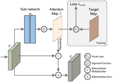
Figure 4. The supervised mask-guided attention network.

3.3. Anchor-free Detection Head

The proposed model can learn a dense mask-guided 2D feature map $G$ in $C_{2}\times L\times W$ dimension from the point cloud. The height information is retained in the 2D feature map by flatting the features from the height dimension into the channel dimension. Inspired by (Zhou et al., 2019b), we construct a new single-stage anchor-free 3D detection head. The $K$-class object detection task is decomposed into three sub-tasks: $K$-class center point classification in the BEV, 3D bounding box regression based on the center points, and estimation of the IoU-based detection confidence. The third part of Fig. 2 shows three parallel heads in a structure similar to the sub-network $\phi_{s}$.

Center point classification. The center point classification head treats the objects as center points. Given the 2D feature map $G\in\mathbb{R}^{C_{2}\times L\times W}$ in the BEV, a heatmap $\hat{P}\in{\left[0,1\right]}^{K\times L\times W}$ is predicted to represent the probability of the center point of each object. The local peaks of the $k$-th channel can be detected as the center points representing the objects of class $k$. And the center point can be directly decoded as the object’s center coordinates $(x,y)$ in the BEV.

The target heatmap $P\in{\left[0,1\right]}^{K\times L\times W}$ can be generated following (Law and Deng, 2018; Zhou et al., 2019b). For each ground truth bounding box of class $k$, the pixel index $\tilde{p}\in\mathbb{R}^{2}$ of the center point $p\in\mathbb{R}^{2}$ on the feature map can be calculated as $\tilde{p}=\lfloor\frac{p}{R}\rfloor$, where $R$ is the output stride. Then a 2D Gaussian exp$(-\frac{(x-\tilde{p_{x}})^{2}+(y-\tilde{p_{y}})^{2}}{2\sigma_{p}^{2}})$ is placed around $\tilde{p}$ to form the target heatmap, where $\sigma_{p}$ is a box-size adaptive standard deviation (Law and Deng, 2018). Only the pixels $\tilde{p}$ at center points are positive, and all other pixels are negative. We use a variant of focal loss to supervise the center classification task as:

(2) $$L_{\text{cls}}=\frac{-1}{N}\sum_{i}\left\{\begin{array}[]{ll}\left(1-\hat{P}_{i}\right)^{\alpha}\log\left(\hat{P}_{i}\right)&\text{ if }{P}_{i}=1,\\ \left(1-{P}_{i}\right)^{\beta}\hat{P}_{i}^{\alpha}\log\left(1-\hat{P}_{i}\right)&\text{ otherwise, }\end{array}\right.$$

where $i$ indexes the pixel location on the heatmap, $N$ is the number of objects, and the hyperparameters $\alpha$ and $\beta$ are selected as $\alpha=2$ and $\beta=4$ (Law and Deng, 2018). Please refer to Fig. 7.(h) - (j) for a clear visualization.

3D Bounding box regression. The 3D object detection locates an object as $(x,y,z,l,w,h,\theta)$, where $(x,y,z)$, $(l,w,h)$, and $\theta$ are denoted as the 3D position coordinates, 3D bounding box size, and the rotation angle of the object.

Although the $(x,y)$ can be decoded from the integer coordinates of the detected center point from the 2D feature map, we can predict an offset $({\Delta x},{\Delta y})$ to compensate for the difference between the actual floating-point coordinates and the integer coordinates of the center point. Since the height information is still retained in the 2D feature map, the coordinate $z$ and the size $(l,w,h)$ are directly regressed. The predictions of the offset $({\Delta x},{\Delta y})$, the coordinate $z$ and the size $(l,w,h)$ are all trained with the L1 loss:

(3) $$L_{\text{l1}}=\frac{1}{N}\sum_{\tilde{p}}\left|\hat{A}_{\tilde{p}}-A_{\tilde{p}}\right|,$$

where only the center point locations $\tilde{p}$ on the prediction map $\hat{A}$ and that on the target map $A$ are computed for the loss. All other locations are ignored.

To ease the regression of the rotation angle without any predefined oriented anchors, we divide $(0,2\pi)$ into $b$ bins and use the bin-res loss (Shi et al., 2019) to conduct the supervision. The model first roughly classifies which bin the $\theta$ is in, and then finely regresses the residuals in this bin. For each center point location $\tilde{p}$, the rotation angle loss $L_{\text{rot},\tilde{p}}$ can be composed of the bin classification loss $L^{\text{bin}}_{\text{rot}}$ and the residual regression loss $L^{\text{res}}_{\text{rot}}$ as

(4) $$L_{\text{rot},\tilde{p}}=L^{bin}_{\text{rot}}(\hat{R}^{\text{bin}}_{\tilde{p}},R^{\text{bin}}_{\tilde{p}})+L^{\text{res}}_{\text{rot}}(\hat{R}^{\text{res}}_{\tilde{p}},R^{\text{res}}_{\tilde{p}}),$$

where $\hat{R}^{\text{bin}}$ and $\hat{R}^{\text{res}}$ are predicted bin classes and residuals while $R^{\text{bin}}$ and $R^{\text{res}}$ are their targets. The total rotation angle loss of $N$ objects can be formulated as

(5) $$L_{\text{rot}}=\frac{1}{N}\sum_{\tilde{p}}L_{\text{rot},\tilde{p}}.$$

Moreover, a corner loss is used to supervise all items related to the 3D bounding box as a whole. The corner loss $L_{\text{corner}}$ is defined as the L2 distance between the eight corners of the predicted bounding box and the assigned ground truth as

(6) $$L_{\text{corner}}=\frac{1}{N}\sum_{\tilde{p}}(\sum_{k=1}^{8}\left\|\hat{B}_{\tilde{p},k}-B_{\tilde{p},k}\right\|),$$

where $\tilde{p}$ indicates that the $L_{\text{corner}}$ only considers the bounding boxes regressed from the center point locations. Therefore, the bounding box prediction is supervised by

(7) $$L_{\text{box}}=\gamma_{1}L_{\text{offset}}+\gamma_{2}L_{\text{z-coord}}+\gamma_{3}L_{\text{size}}+\gamma_{4}L_{\text{rot}}+\gamma_{5}L_{\text{corner}},$$

where $\gamma_{1}\sim\gamma_{5}$ are the constant coefficients to balance each loss.

IoU-based detection confidence recalibration. To detect an object with a confidence score, we can directly use the local peak value on the center point classification heatmap as detection confidence of the object (Zhou et al., 2019b). The model can achieve better detection performance when the detection confidence is positively correlated with the IoU of the predicted bounding box (Jiang et al., 2018; Li et al., 2020b). However, the local peak values on the classification heatmap are all close to 1 and have a low positive correlation with the actual IoUs of the predicted bounding boxes. To improve the correlation, a parallel confidence estimation head is designed to predict IoU-based confidence. The detection confidence is re-calibrated from the classification score to the IoU-based confidence.

The training samples and targets for the confidence estimation head are obtained automatically during the training of the network. The top $M$ local peaks on the predicted classification heatmap are utilized to select the corresponding $M$ predicted bounding boxes as the confidence training samples. $M$ is a hyperparameter we chose to balance the training samples with IoUs greater than zero and equal to zero. For the $m$-th bounding box, we calculate the 3D IoUs between the $m$-th bounding box and all ground truth bounding boxes, and then assign the largest one as its actual IoU denoted as $IoU_{m}$. We follow (Shi et al., 2020a) to normalize each confidence training target $c_{m}$ between $\left[0,1\right]$ as:

(8) $$c_{m}=\text{min}(1,\text{max}(0,2IoU_{m}-0.5)).$$

The confidence estimation head is then trained to minimize the cross-entropy loss computed from the predicted confidence $\hat{c}_{m}$ and its target $c_{m}$ as:

(9) $$L_{\text{iou}}=\frac{-1}{M}\sum_{m}(c_{m}\text{log}(\hat{c}_{m})+(1-c_{m})\text{log}(1-\hat{c}_{m})).$$

In the inference stage, the confidence $\hat{c}$ predicted by the network can be directly assigned to the corresponding predicted bounding box as the detection confidence score.

The two-stage methods PV-RCNN (Shi et al., 2020a) and STD (Yang et al., 2019b) also learn the IoUs of the proposal boxes to guide the NMS. Note that there are two main differences in our method: 1) PV-RCNN and STD require the actual IoUs of the proposal boxes as the training target for their confidence branches in the second stage. However, there are no proposal boxes or anchor boxes in our one-stage anchor-free methods. Instead, we use IoUs of the predicted boxes as training targets for IoU prediction in a parallel regression head. 2) PV-RCNN and STD use the predicted IoUs for refined boxes de-redundancy in NMS, while we only re-calibrate the detection confidence using the predicted IoUs without NMS.

Training loss. Our network is trained end-to-end with a multi-task loss $L_{\text{total}}$ as Eq.(10), which is equally contributed by the center point classification loss $L_{\text{cls}}$, the 3D bounding box regression loss $L_{\text{box}}$, the IoU-based confidence training loss $L_{\text{iou}}$, and the mask-guided attention training loss $L_{\text{sem}}$.

(10) $$L_{\text{total}}=L_{\text{cls}}+L_{\text{box}}+L_{\text{iou}}+L_{\text{sem}}.$$

4. Experiment

4.1. Datasets

KITTI Dataset. KITTI 3D object detection benchmark (KITTI, 2021) is widely used for 3D object detection evaluation. The KITTI dataset (Geiger et al., 2012) provides 7481 training samples and 7518 testing samples with objects of three classes: car, pedestrian, and cyclist. The training samples are generally divided into the train split set (3712 samples) and the val split set (3769 samples) for experiments (Chen et al., 2017; Zhou and Tuzel, 2018; Shi et al., 2019). For each class, the detection performance is evaluated as the Average Precision (AP) based on three difficulty levels: easy, moderate, and hard. Following the official evaluation protocol, we calculate the $\text{AP}_{\text{3D}}$ with 40 recall positions as the evaluation metric.

Waymo Open Dataset. The newly released Waymo Open Dataset (Sun et al., 2020a) is the currently largest public dataset for autonomous driving. Waymo contains $\sim$158K point cloud training samples and $\sim$40K point cloud validation samples. The objects in Waymo are divided into two levels: LEVEL_1 for boxes with more than five LiDAR points, and LEVEL_2 for boxes with at least one LiDAR point. The official evaluation tool provides metrics of $\text{AP}_{\text{3D}}$ and $\text{AP}_{\text{BEV}}$ for the 3D and BEV detection.

4.2. Implement Details

Network architecture. Since the objects in KITTI are only annotated in the camera Field of Vision (FOV), the quantization step $d$ is set as $(0.05,0.05,0.1)$ meters to voxelize the KITTI point clouds within the range of $\left[0,70.4\right]\times\left[-40,40\right]\times\left[-3,1\right]$ meters along the $X$, $Y$, $Z$ axis, resulting in an initial spatial resolution $(L_{0},W_{0},H_{0})$ of $(1408,1600,40)$. For the full $360\mathrm{°}$-field detection in Waymo, we voxelize the Waymo point clouds within the range of $\left[-75.2,75.2\right]\times\left[-75.2,75.2\right]\times\left[-2,4\right]$ meters with the quantization step $d$ as $(0.1,0.1,0.15)$ along the $X$, $Y$, $Z$ axis, resulting in an initial spatial resolution $(L_{0},W_{0},H_{0})$ of $(1504,1504,40)$. The ResVoxelNet downsamples the feature volumes with $1\times$, $2\times$ $4\times$, $8\times$ while increases the feature dimension as 16, 32, 64, 128. The ADFA module maintains the $8\times$ downsampled resolution $(L,W)$ of (176, 200) or (188, 188) with a feature dimension $C_{2}$ of 256 for KITTI and Waymo models. Each head is implemented by two convolutions with stride of 1: a $3\times 3$ convolution with 128 channels, and a $1\times 1$ convolution with different numbers of channels for different output values.

Training details. Our model is trained from scratch in an end-to-end manner with the AdamW (Loshchilov and Hutter, 2017) optimizer and one-cycle policy (Smith and Topin, 2019) with LR max 0.01, division factor 10, momentum ranges from 0.95 to 0.85, weight decay 0.01. For KITTI, the model is trained for 50 epochs with batch size 8 on a Tesla V100 GPU. For Waymo, the model is trained for 36 epochs with batch size 36 on 4 Tesla V100 GPUs. To avoid overfitting during the training process, four commonly used data augmentation strategies are used to avoid overfitting: ground truth sampling (Yan et al., 2018), random flipping along the $X$ axis, global scaling with a random scaling factor in $[0.95,1.05]$, global rotation around the $Z$ axis with a random angle in $[-\frac{\pi}{4},\frac{\pi}{4}]$.

Inference details. For the inference, the Non-maximum suppression (NMS) post-processing process is no longer needed (Zhou et al., 2019b). A $3\times 3$ max-pooling operation is applied to extract the local peaks on each channel of the center point classification heatmap. The detection results at the top 50 or 200 local peaks are kept as candidates for KITTI and Waymo since the Waymo point cloud contains more object instances than KITTI. A threshold $\mu_{cls}$ of 0.5 is then applied to filter the negative detection results.

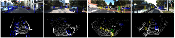
Figure 5. Qualitative results of our method on the KITTI test set. We show the predicted 3D bounding boxes of cars (blue), cyclists (green) and pedestrians (yellow) on both the image and the point cloud. Best viewed with color and zooming in.

Table 1. Performance comparison on car class of the KITTI test set. Methods are divided into two types: two-stage and single-stage. Blue numbers are results for the best detection performance. Bold numbers denote the top-2 results for single-stage point cloud detectors.

Method	Sensor	Anchor	$\text{AP}_{\text{3D}}$
			Easy	Mod.	Hard
MV3D(Chen et al., 2017)	LiDAR + RGB	$\surd$	74.97	63.63	54.00
F-PointNet(Qi et al., 2018)	LiDAR + RGB	$\surd$	82.19	69.79	60.59
PointPainting(Vora et al., 2020)	LiDAR + RGB	$\surd$	82.11	71.70	67.08
AVOD(Ku et al., 2018)	LiDAR + RGB	$\surd$	83.07	71.76	65.73
PI-RCNN(Xie et al., 2020)	LiDAR + RGB	$\surd$	84.37	74.82	70.03
CLOCs_PointCas(Pang et al., 2020)	LiDAR + RGB	$\surd$	87.50	76.68	71.20
MMF(Liang et al., 2019)	LiDAR + RGB	$\surd$	88.40	77.43	70.22
PointRCNN(Shi et al., 2019)	LiDAR only	$\surd$	86.96	75.64	70.70
Fast PointRCNN(Chen et al., 2019)	LiDAR only	$\surd$	85.29	77.40	70.24
STD(Yang et al., 2019b)	LiDAR only	$\surd$	87.95	79.71	75.09
Part-A2(Shi et al., 2020b)	LiDAR only	$\surd$	87.81	78.49	73.51
PV-RCNN(Shi et al., 2020a)	LiDAR only	$\surd$	90.25	81.43	76.82
VoxelNet(Zhou and Tuzel, 2018)	LiDAR only	$\surd$	78.82	64.17	57.51
SECOND(Yan et al., 2018)	LiDAR only	$\surd$	83.34	72.55	65.82
PointPillars(Lang et al., 2019)	LiDAR only	$\surd$	82.58	74.31	68.99
SCNet(Wang et al., 2019)	LiDAR only	$\surd$	83.34	73.17	67.93
TANet(Liu et al., 2020)	LiDAR only	$\surd$	84.39	75.94	68.82
Associate-3Ddet(Du et al., 2020)	LiDAR only	$\surd$	85.99	77.40	70.53
Point-GNN(Shi and Rajkumar, 2020)	LiDAR only	$\surd$	88.33	79.47	72.29
HotSpotNet(Chen et al., 2020)	LiDAR only	$\times$	87.60	78.31	73.34
Ours	LiDAR only	$\times$	88.16	79.68	72.39

Table 2. $\text{AP}_{\text{3D}}$ comparison on cyclist and pedestrian classes of the KITTI test set. Methods are divided into two types: two-stage and single-stage. Blue numbers are results for the best detection performance. Bold numbers denote the top-2 results for single-stage point cloud detectors.

Method	Anchor	Cyclist			Pedestrian
		Easy	Mod.	Hard	Easy	Mod.	Hard
AVOD-FPN(Ku et al., 2018)	$\surd$	63.76	50.55	44.93	50.46	42.27	39.04
F-PointNet(Qi et al., 2018)	$\surd$	72.27	56.12	49.01	50.53	42.15	38.08
STD(Yang et al., 2019b)	$\surd$	78.69	61.59	55.30	53.29	42.47	38.35
PointPainting(Vora et al., 2020)	$\surd$	77.63	63.78	55.89	50.32	40.97	37.87
PV-RCNN(Shi et al., 2020a)	$\surd$	78.60	63.71	57.65	N/A	N/A	N/A
SCNet(Wang et al., 2019)	$\surd$	67.98	50.79	45.15	47.83	38.66	35.70
PointPillars(Lang et al., 2019)	$\surd$	77.10	58.65	51.92	51.45	41.92	38.89
SemanticVoxels(Fei et al., 2020)	$\surd$	N/A	N/A	N/A	50.90	42.19	39.52
TANet(Liu et al., 2020)	$\surd$	75.70	59.44	52.53	53.72	44.34	40.49
Ours	$\times$	80.64	63.43	55.15	50.65	43.09	39.65

Figure 6. Latency comparison: $\text{AP}_{\text{3D}}$ on moderate car class of KITTI test set (top consideration in KITTI) vs. inference time in milliseconds.

4.3. Results on KITTI Dataset

Fig. 5 shows the qualitative results of our method on the KITTI test set. Tab. 1 and Tab. 2 present the performance comparison between our anchor-free single-stage method and the most existing state-of-the-art methods on the KITTI test set. For the main considered car class shown in Tab. 1, our method makes $\text{AP}_{\text{3D}}$ margins of 0.56%, 1.37% on the easy and moderate levels compared with the latest anchor-free method HotSpotNet (Chen et al., 2020), which shows that the object center is more robust than the various hotspots lying on the object surface. For $\text{AP}_{\text{3D}}$ on the three levels, our method outperforms the state-of-the-art anchor-based single-stage point cloud detectors. Our method still outperforms the most two-stage methods, and achieves better performance with the STD (Yang et al., 2019b) and Part-A2 (Shi et al., 2020b) on the easy level. Our method also has significant improvement when compared to MV3D (Chen et al., 2017) and AVOD (Ku et al., 2018), indicating that the feature level 3D-to-2D transformation effectively avoids the information loss caused by the 3D-to-2D data conversion at the input level.

In addition, our method performs well on small objects like cyclists and pedestrians, as shown in Tab. 2. Most methods do not provide results for cyclists and pedestrians, due to the difficulty of detecting small objects. For cyclists, our method not only outperforms the single-stage detectors, but also achieves better performance against the two-stage anchor-based PV-RCNN (Shi et al., 2020a) on the easy level. The results show the effectiveness of our method.

Latency comparison. Fig. 6 demonstrates the latency comparison that is performed on the same machine with the same settings. Since most methods do not report the inference time, we have re-implemented the methods with official codes publicly available. Our method saves almost half of the inference time, while it achieves comparable performance with PV-RCNN (Shi et al., 2020a) and it is even better than other two-stage methods Part-A2 (Shi et al., 2020b) and PointRCNN (Shi et al., 2019).

4.4. Results on Waymo Open Dataset

We evaluate the performance on the Waymo Open Dataset for both LEVEL_1 and LEVEL_2, and compare the $\text{AP}_{\text{3D}}$ and $\text{AP}_{\text{BEV}}$ with the top-performing methods. Tab. 3 shows that we achieve better performance than the existing methods with 71.98% $\text{AP}_{\text{3D}}$ and 87.15% $\text{AP}_{\text{BEV}}$ on the most commonly used LEVEL_1. Besides, our method outperforms PV-RCNN on the BEV of LEVEL_2. The improvements on the $\text{AP}_{\text{BEV}}$ demonstrate the effectiveness of our method for detecting the objects as the center points in the BEV.

Table 3. Performance comparison on the Waymo validation for vehicle detection. The top-1 results are in bold.

Difficulty	Method	Stage	Overall	[0, 30)m	[30, 50)m	[50, Inf)m
LEVEL_1			$\text{AP}_{\text{3D}}$
	PV-RCNN(Shi et al., 2020a)	2	70.30	91.92	69.21	42.17
	PointPillars(Lang et al., 2019)	1	56.62	81.01	51.75	27.94
	MVF(Zhou et al., 2019a)	1	62.93	86.30	60.02	36.02
	Pillar-OD(Wang et al., 2020)	1	69.80	88.53	66.50	42.93
	Ours	1	71.98	91.85	70.58	48.04
			$\text{AP}_{\text{BEV}}$
	PV-RCNN(Shi et al., 2020a)	2	82.96	97.35	82.99	64.97
	PointPillars(Lang et al., 2019)	1	75.57	92.10	74.06	55.47
	MVF(Zhou et al., 2019a)	1	80.40	93.59	79.21	63.09
	Pillar-OD(Wang et al., 2020)	1	87.11	95.78	84.74	72.12
	Ours	1	87.15	97.42	86.80	73.92
LEVEL_2			$\text{AP}_{\text{3D}}$
	PV-RCNN(Shi et al., 2020a)	2	65.36	91.58	65.13	36.46
	Ours	1	64.78	88.85	64.64	36.17
			$\text{AP}_{\text{BEV}}$
	PV-RCNN(Shi et al., 2020a)	2	77.45	94.64	80.39	55.39
	Ours	1	77.85	94.39	80.87	59.16

4.5. Ablation Study

Extensive ablation experiments are conducted to analyze each individual component of our methods. Following the existing works (Shi et al., 2020a; Shi and Rajkumar, 2020; Yan et al., 2018; Yang et al., 2019b; Shi et al., 2019; Xie et al., 2020), we train the models on the KITTI trian split set with the same training settings and adopt the $\text{AP}_{\text{3D}}$ on the car class of KITTI val split set as the performance evaluation metric. Besides, we also perform each ablation experiment on the Waymo vehicle detection and report the $\text{AP}_{\text{3D}}$ on the Waymo validation for stability. In each table, the best performance is marked in bold.

ADFA module. Our ADFA module consists of two main components: the mask-guided attention and the deformable convolutional tower that can be assembled with or without the deformable convolutions. As shown in Tab. 4, the performance drops significantly when we remove the entire ADFA module, indicating the importance of the ADFA module. When adding a vanilla convolutional tower combined with multiple receptive fields, the performance becomes better, especially for the moderate and hard levels on KITTI. After the receptive fields are adaptively adjusted by the deformable convolutions and the feature maps are enhanced by the mask-guided attention, the performance becomes better on both KITTI and Waymo. Compared with the input feature map in Fig. 7.(c), the output feature map in Fig. 7.(d) becomes much denser and more focused on the entire object. With the dense mask-guided feature map provided by the ADFA module, our model achieves the best performance as shown in the last row of Tab. 4.

Table 4. Effectiveness ($\text{AP}_{\text{3D}}$) of each individual component in the ADFA module. “Conv.”, “DCN”, and “Att.” denote 2D convolutional tower, deformable convolution, and mask-guided attention, respectively.

Conv.	DCN	Att.	KITTI			Waymo
			Easy	Mod.	Hard	LEVEL_1	LEVEL_2
$\times$	$\times$	$\times$	89.87	78.55	75.92	70.29	61.20
$\surd$	$\times$	$\times$	89.81	80.97	78.23	71.17	62.13
$\surd$	$\surd$	$\times$	90.27	81.14	78.40	71.42	64.24
$\surd$	$\surd$	$\surd$	91.86	83.29	78.51	71.98	64.78

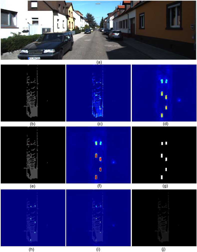
Figure 7. Visualization of the ADFA module and center point classification. (a) RGB image. (b) Occupancy grids of the sparse 3D feature volume in the BEV. (c) Input feature map of ADFA module. (d) Output feature map of ADFA module. (e) Occupancy grids with red points of object centers. (f) Predicted mask-guided attention map. (g) Binary segmentation mask. (h) Target and (i) predicted heatmap of center point classification. (j) The local peaks from the predicted heatmap and the target heatmap are colored in blue and red, and become purple if they overlap.

Table 5. Effectiveness of supervised mask-guided attention.

Supervision	Reweighting	KITTI			Waymo
		Easy	Mod.	Hard	LEVEL_1	LEVEL_2
$\times$	$\times$	90.27	81.14	78.40	71.42	64.24
$\surd$	$\times$	90.52	83.09	78.22	71.57	64.39
$\surd$	$\surd$	91.86	83.29	78.51	71.98	64.78

Supervised mask-guided attention. Tab. 5 validates the effectiveness of supervised mask-guided attention. In multi-task learning, the related auxiliary tasks usually facilitate the learning of the main task. As shown in the second row of Tab. 5, the mask-guided supervision contributes to the improvement on KITTI and Waymo. When we further use the mask-guided attention map to penalize the feature map, our method achieves much higher $\text{AP}_{\text{3D}}$. Fig. 7.(f) illustrates the predicted mask-guided attention map.

Detection confidence recalibration. We investigate the importance of the IoU-based detection confidence recalibration in three models with different settings shown in Tab. 6 and Tab. 7. From model A to model B, the joint learning of the auxiliary IoU-based confidence estimation task brings the slight improvements of 0.72%, 0.61%, 0.45% $\text{AP}_{\text{3D}}$ on KITTI and 0.56%, 0.53% $\text{AP}_{\text{3D}}$ on Waymo. The comparison between the model B and C with the same trained network demonstrates that the proposed IoU-based detection confidence recalibration scheme significantly improves the model B with 2.90%, 2.17%, 1.50% $\text{AP}_{\text{3D}}$ on KITTI and 1.94%, 1.71% $\text{AP}_{\text{3D}}$ on Waymo, respectively. Moreover, we calculate the correlation between the confidence of the detection results and their actual 3D IoUs to analyze how the confidence recalibration mechanism works. The highest Pearson Linear Correlation Coefficient (PLCC) and Spearman Rank-order Correlation Coefficient (SRCC) in the third rows of Tab. 6 and Tab. 7 indicates that the recalibrated confidence becomes more relevant to the detection accuracy.

Table 6. Effectiveness of detection confidence recalibration on KITTI. “Head${}_{\text{iou}}$” and “Recalib.” denote IoU-based detection confidence estimation head and recalibration.

	Setting		PLCC	SRCC	KITTI
	Head${}_{\text{iou}}$	Recalib.			Easy	Mod.	Hard
A	$\times$	$\times$	0.478	0.552	88.24	80.51	76.56
B	$\surd$	$\times$	0.485	0.556	88.96	81.12	77.01
C	$\surd$	$\surd$	0.547	0.649	91.86	83.29	78.51

Table 7. Effectiveness of detection confidence recalibration on Waymo.

	Setting		PLCC	SRCC	Waymo
	Headiou	Recalib.			LEVEL_1	LEVEL_2
A	$\times$	$\times$	0.337	0.339	69.48	62.54
B	$\surd$	$\times$	0.340	0.342	70.04	63.07
C	$\surd$	$\surd$	0.579	0.689	71.98	64.78

Table 8. Detection performance $\text{AP}_{\text{3D}}$ with different number ($M$) of training samples of $\text{Head}_{\text{iou}}$ on KITTI.

M	KITTI			Mean
	Easy	Mod.	Hard
4	90.22	80.74	78.10	83.02
8	90.33	83.10	78.56	83.99
16	92.03	83.16	78.42	84.53
24	91.86	83.29	78.51	84.55
32	90.35	83.24	78.45	84.01
40	90.37	83.22	78.36	83.98
48	90.39	81.42	78.50	83.43

Table 9. Detection performance $\text{AP}_{\text{3D}}$ with different number ($M$) of training samples of $\text{Head}_{\text{iou}}$ on Waymo.

M	Waymo		Mean
	LEVEL_1	LEVEL_2
32	71.39	62.32	66.35
56	71.54	64.36	67.95
80	71.90	64.70	68.30
104	71.98	64.78	68.38
128	71.94	64.74	68.34
152	71.67	64.48	68.09
176	71.12	62.07	66.60

Hyperparameter $M$. As shown in Tab. 4.5, the performance is relatively stable with the $M$ around 24 on KITTI but drops as the $M$ becomes larger or smaller. Generally, each scene of the KITTI dataset does not contain many object instances. A large $M$ may include too many negative detection results with IoUs of zero, which causes that the IoU training loss on the positive detection results is overwhelmed by that on the negative detection results. A small $M$ may include many training samples with positive IoUs, which is not conducive to the IoU-based confidence estimation head for distinguishing the false positives with IoUs of zero during the inference. According to the highest mean $\text{AP}_{\text{3D}}$ shown in Tab. 4.5 and Tab. 4.5, we choose $M$ as 24 and 104 for KITTI and Waymo, respectively. The reason why the $M$ on Waymo is larger than KITTI is that the full $360\mathrm{°}$-field scene in Waymo contains more object instances than the camera FOV in KITTI.

5. Conclusion

In this work, we propose a novel anchor-free single-stage 3D detection framework. The proposed ADFA module enables the center of the object to better perceive the whole object with the adaptive receptive fields and the supervised mask-guided attention. We design an anchor-free 3D detection head to get rid of hand-crafted anchors and NMS for box de-redundancy without sacrificing the detection accuracy. We propose an IoU-based detection confidence re-calibration scheme to improve the correlation between the detection confidence and the detection accuracy, which significantly improves the 3D object detection performance. Experimental results on the widely used KITTI dataset and the newly released large-scale Waymo Open Dataset demonstrate that our method achieves better performance than the anchor-based 3D object detectors, and each individual component in our method is effective with significant performance gains.

- (1)
- Cai and Vasconcelos (2018) Zhaowei Cai and Nuno Vasconcelos. 2018. Cascade R-CNN: Delving Into High Quality Object Detection. In 2018 IEEE/CVF Conference on Computer Vision and Pattern Recognition (CVPR). 6154–6162.
- Chen et al. (2020) Qi Chen, Lin Sun, Zhixin Wang, Kui Jia, and Alan Yuille. 2020. Object as Hotspots: An Anchor-Free 3D Object Detection Approach via Firing of Hotspots. In European Conference on Computer Vision (ECCV). 68–84.
- Chen et al. (2017) Xiaozhi Chen, Huimin Ma, Ji Wan, Bo Li, and Tian Xia. 2017. Multi-view 3D Object Detection Network for Autonomous Driving. In 2017 IEEE Conference on Computer Vision and Pattern Recognition (CVPR). 6526–6534.
- Chen et al. (2019) Yilun Chen, Shu Liu, Xiaoyong Shen, and Jiaya Jia. 2019. Fast Point R-CNN. In 2019 IEEE/CVF International Conference on Computer Vision (ICCV). 9775–9784.
- Dai et al. (2020) Hang Dai, Shujie Luo, Yong Ding, and Ling Shao. 2020. Commands for autonomous vehicles by progressively stacking visual-linguistic representations. In European Conference on Computer Vision (ECCV). Springer, 27–32.
- Dai et al. (2017) Jifeng Dai, Haozhi Qi, Yuwen Xiong, Yi Li, Guodong Zhang, Han Hu, and Yichen Wei. 2017. Deformable Convolutional Networks. In 2017 IEEE International Conference on Computer Vision (ICCV). 764–773.
- Du et al. (2020) Liang Du, Xiaoqing Ye, Xiao Tan, Jianfeng Feng, Zhenbo Xu, Errui Ding, and Shilei Wen. 2020. Associate-3Ddet: Perceptual-to-Conceptual Association for 3D Point Cloud Object Detection. In 2020 IEEE/CVF Conference on Computer Vision and Pattern Recognition (CVPR). 13326–13335.
- Duan et al. (2019) Kaiwen Duan, Song Bai, Lingxi Xie, Honggang Qi, Qingming Huang, and Qi Tian. 2019. CenterNet: Keypoint Triplets for Object Detection. In 2019 IEEE/CVF International Conference on Computer Vision (ICCV). 6568–6577.
- Fei et al. (2020) Juncong Fei, Wenbo Chen, Philipp Heidenreich, Sascha Wirges, and Christoph Stiller. 2020. SemanticVoxels: Sequential Fusion for 3D Pedestrian Detection using LiDAR Point Cloud and Semantic Segmentation. In IEEE International Conference on Multisensor Fusion and Integration for Intelligent Systems. IEEE, 185–190.
- Feng et al. (2020) Tuo Feng, Licheng Jiao, Hao Zhu, and Long Sun. 2020. A Novel Object Re-Track Framework for 3D Point Clouds. In MM ’20: The 28th ACM International Conference on Multimedia. ACM, 3118–3126.
- Geiger et al. (2012) Andreas Geiger, Philip Lenz, and Raquel Urtasun. 2012. Are We Ready for Autonomous Driving? The KITTI Vision Benchmark Suite. In 2012 IEEE Conference on Computer Vision and Pattern Recognition (CVPR). 3354–3361.
- Graham (2015) Ben Graham. 2015. Sparse 3D Convolutional Neural Networks. In 2015 British Machine Vision Conference (BMVC). 150.1–150.9.
- Graham et al. (2018) Benjamin Graham, Martin Engelcke, and Laurens van der Maaten. 2018. 3D Semantic Segmentation With Submanifold Sparse Convolutional Networks. In 2018 IEEE/CVF Conference on Computer Vision and Pattern Recognition (CVPR). 9224–9232.
- He et al. (2020) Chenhang He, Hui Zeng, Jianqiang Huang, Xian-Sheng Hua, and Lei Zhang. 2020. Structure Aware Single-Stage 3D Object Detection From Point Cloud. In 2020 IEEE/CVF Conference on Computer Vision and Pattern Recognition (CVPR). 11870–11879.
- He et al. (2017) Kaiming He, Georgia Gkioxari, Piotr Dollár, and Ross B. Girshick. 2017. Mask R-CNN. In 2017 IEEE International Conference on Computer Vision (ICCV). 2980–2988.
- He et al. (2016) Kaiming He, Xiangyu Zhang, Shaoqing Ren, and Jian Sun. 2016. Deep Residual Learning for Image Recognition. In 2016 IEEE Conference on Computer Vision and Pattern Recognition (CVPR). 770–778.
- Hsu (2019) Winston H. Hsu. 2019. Learning from 3D (Point Cloud) Data. In MM ’19: The 27th ACM International Conference on Multimedia. ACM, 2697–2698.
- Jiang et al. (2018) Borui Jiang, Ruixuan Luo, Jiayuan Mao, Tete Xiao, and Yuning Jiang. 2018. Acquisition of Localization Confidence for Accurate Object Detection. In European Conference on Computer Vision (ECCV). 784–799.
- KITTI (2021) KITTI. 2021. KITTI Leaderboard of 3D Object Detection Benchmark. http://www.cvlibs.net/datasets/kitti/eval_object.php?obj_benchmark=3d
- Ku et al. (2018) Jason Ku, Melissa Mozifian, Jungwook Lee, Ali Harakeh, and Steven L. Waslander. 2018. Joint 3D Proposal Generation and Object Detection from View Aggregation. In 2018 IEEE/RSJ International Conference on Intelligent Robots and Systems (IROS). 1–8.
- Lang et al. (2019) Alex H. Lang, Sourabh Vora, Holger Caesar, Lubing Zhou, Jiong Yang, and Oscar Beijbom. 2019. PointPillars: Fast Encoders for Object Detection From Point Clouds. In 2019 IEEE/CVF Conference on Computer Vision and Pattern Recognition (CVPR). 12689–12697.
- Law and Deng (2018) Hei Law and Jia Deng. 2018. CornerNet: Detecting Objects as Paired Keypoints. In European Conference on Computer Vision (ECCV), Vol. 11218. 765–781.
- Li et al. (2020a) Jiale Li, Shujie Luo, Ziqi Zhu, Hang Dai, Andrey S Krylov, Yong Ding, and Ling Shao. 2020a. 3D IoU-Net: IoU guided 3D object detector for point clouds. arXiv preprint arXiv:2004.04962 (2020).
- Li et al. (2021) Jiale Li, Yu Sun, Shujie Luo, Ziqi Zhu, Hang Dai, Andrey S Krylov, Yong Ding, and Ling Shao. 2021. P2V-RCNN: Point to Voxel Feature Learning for 3D Object Detection from Point Clouds. IEEE Access (2021).
- Li et al. (2020b) Xiang Li, Wenhai Wang, Lijun Wu, Shuo Chen, Xiaolin Hu, Jun Li, Jinhui Tang, and Jian Yang. 2020b. Generalized Focal Loss: Learning Qualified and Distributed Bounding Boxes for Dense Object Detection. In Conference on Neural Information Processing Systems (NeurIPS).
- Liang et al. (2019) Ming Liang, Bin Yang, Yun Chen, Rui Hu, and Raquel Urtasun. 2019. Multi-Task Multi-Sensor Fusion for 3D Object Detection. In 2019 IEEE/CVF Conference on Computer Vision and Pattern Recognition (CVPR). 7337–7345.
- Lin et al. (2017) Tsung-Yi Lin, Piotr Dollár, Ross B. Girshick, Kaiming He, Bharath Hariharan, and Serge J. Belongie. 2017. Feature Pyramid Networks for Object Detection. In 2017 IEEE Conference on Computer Vision and Pattern Recognition (CVPR). 936–944.
- Lin et al. (2020) Tsung-Yi Lin, Priya Goyal, Ross B. Girshick, Kaiming He, and Piotr Dollár. 2020. Focal Loss for Dense Object Detection. IEEE Transactions on Pattern Analysis and Machine Intelligence 42, 2 (2020), 318–327.
- Liu et al. (2016) Wei Liu, Dragomir Anguelov, Dumitru Erhan, Christian Szegedy, Scott E. Reed, Cheng-Yang Fu, and Alexander C. Berg. 2016. SSD: Single Shot Multibox Detector. In European Conference on Computer Vision (ECCV). Springer, 21–37.
- Liu et al. (2020) Zhe Liu, Xin Zhao, Tengteng Huang, Ruolan Hu, Yu Zhou, and Xiang Bai. 2020. TANet: Robust 3D Object Detection from Point Clouds with Triple Attention. In 2020 AAAI Conference on Artificial Intelligence (AAAI). 11677–11684.
- Loshchilov and Hutter (2017) Ilya Loshchilov and Frank Hutter. 2017. Fixing Weight Decay Regularization in Adam. CoRR abs/1711.05101 (2017). arXiv:1711.05101
- Luo et al. (2020) Shujie Luo, Hang Dai, Ling Shao, and Yong Ding. 2020. C4AV: Learning Cross-Modal Representations from Transformers. In European Conference on Computer Vision (ECCV). Springer, 33–38.
- Luo et al. (2021) Shujie Luo, Hang Dai, Ling Shao, and Yong Ding. 2021. M3DSSD: Monocular 3D single stage object detector. In IEEE/CVF Conference on Computer Vision and Pattern Recognition (CVPR). 6145–6154.
- Pang et al. (2020) Su Pang, Daniel D. Morris, and Hayder Radha. 2020. CLOCs: Camera-LiDAR Object Candidates Fusion for 3D Object Detection. In IEEE/RSJ International Conference on Intelligent Robots and Systems (IROS). 10386–10393.
- Qi et al. (2018) Charles R. Qi, Wei Liu, Chenxia Wu, Hao Su, and Leonidas J. Guibas. 2018. Frustum PointNets for 3D Object Detection from RGB-D Data. In 2018 IEEE/CVF Conference on Computer Vision and Pattern Recognition (CVPR). 918–927.
- Qi et al. (2017a) Charles Ruizhongtai Qi, Hao Su, Kaichun Mo, and Leonidas J. Guibas. 2017a. PointNet: Deep Learning on Point Sets for 3D Classification and Segmentation. In 2017 IEEE Conference on Computer Vision and Pattern Recognition (CVPR). 77–85.
- Qi et al. (2017b) Charles Ruizhongtai Qi, Li Yi, Hao Su, and Leonidas J. Guibas. 2017b. PointNet++: Deep Hierarchical Feature Learning on Point Sets in a Metric Space. In Conference on Neural Information Processing Systems (NeurIPS). 5099–5108.
- Qin et al. (2020) Zengyi Qin, Jinglu Wang, and Yan Lu. 2020. Weakly Supervised 3D Object Detection from Point Clouds. In MM ’20: The 28th ACM International Conference on Multimedia. ACM, 4144–4152.
- Redmon et al. (2016) Joseph Redmon, Santosh Kumar Divvala, Ross B. Girshick, and Ali Farhadi. 2016. You Only Look Once: Unified, Real-Time Object Detection. In 2016 IEEE Conference on Computer Vision and Pattern Recognition (CVPR). 779–788.
- Ren et al. (2017) Shaoqing Ren, Kaiming He, Ross B. Girshick, and Jian Sun. 2017. Faster R-CNN: Towards Real-Time Object Detection with Region Proposal Networks. IEEE Transactions on Pattern Analysis and Machine Intelligence 39, 6 (2017), 1137–1149.
- Saputra et al. (2019) Roni Permana Saputra, Nemanja Rakicevic, and Petar Kormushev. 2019. Sim-to-Real Learning for Casualty Detection from Ground Projected Point Cloud Data. In 2019 IEEE/RSJ International Conference on Intelligent Robots and Systems (IROS). 3918–3925.
- Shi et al. (2020a) Shaoshuai Shi, Chaoxu Guo, Li Jiang, Zhe Wang, Jianping Shi, Xiaogang Wang, and Hongsheng Li. 2020a. PV-RCNN: Point-Voxel Feature Set Abstraction for 3D Object Detection. In 2020 IEEE/CVF Conference on Computer Vision and Pattern Recognition (CVPR). 10526–10535.
- Shi et al. (2019) Shaoshuai Shi, Xiaogang Wang, and Hongsheng Li. 2019. PointRCNN: 3D Object Proposal Generation and Detection From Point Cloud. In 2019 IEEE/CVF Conference on Computer Vision and Pattern Recognition (CVPR). 770–779.
- Shi et al. (2020b) Shaoshuai Shi, Zhe Wang, Jianping Shi, Xiaogang Wang, and Hongsheng Li. 2020b. From Points to Parts: 3D Object Detection from Point Cloud with Part-aware and Part-aggregation Network. IEEE Transactions on Pattern Analysis and Machine Intelligence (2020), 1–1.
- Shi and Rajkumar (2020) Weijing Shi and Raj Rajkumar. 2020. Point-GNN: Graph Neural Network for 3D Object Detection in a Point Cloud. In 2020 IEEE/CVF Conference on Computer Vision and Pattern Recognition (CVPR). 1708–1716.
- Smith and Topin (2019) Leslie N. Smith and Nicholay Topin. 2019. Super-convergence: Very Fast Training of Neural Networks Using Large Learning Rates. In Artificial Intelligence and Machine Learning for Multi-Domain Operations Applications, Vol. 11006. 1100612.
- Sun et al. (2020a) Pei Sun, Henrik Kretzschmar, Xerxes Dotiwalla, Aurelien Chouard, Vijaysai Patnaik, Paul Tsui, James Guo, Yin Zhou, Yuning Chai, Benjamin Caine, Vijay Vasudevan, Wei Han, Jiquan Ngiam, Hang Zhao, Aleksei Timofeev, Scott Ettinger, Maxim Krivokon, Amy Gao, Aditya Joshi, Yu Zhang, Jonathon Shlens, Zhifeng Chen, and Dragomir Anguelov. 2020a. Scalability in Perception for Autonomous Driving: Waymo Open Dataset. In 2020 IEEE/CVF Conference on Computer Vision and Pattern Recognition (CVPR). 2443–2451.
- Sun et al. (2020b) Xuebin Sun, Sukai Wang, Miaohui Wang, Shing Shin Cheng, and Ming Liu. 2020b. An Advanced LiDAR Point Cloud Sequence Coding Scheme for Autonomous Driving. In MM ’20: The 28th ACM International Conference on Multimedia. ACM, 2793–2801.
- Tian et al. (2019) Zhi Tian, Chunhua Shen, Hao Chen, and Tong He. 2019. FCOS: Fully Convolutional One-Stage Object Detection. In 2019 IEEE/CVF International Conference on Computer Vision (ICCV). 9626–9635.
- Vora et al. (2020) Sourabh Vora, Alex H. Lang, Bassam Helou, and Oscar Beijbom. 2020. PointPainting: Sequential Fusion for 3D Object Detection. In 2020 IEEE/CVF Conference on Computer Vision and Pattern Recognition (CVPR). 4603–4611.
- Wang et al. (2020) Yue Wang, Alireza Fathi, Abhijit Kundu, David A. Ross, Caroline Pantofaru, Thomas A. Funkhouser, and Justin Solomon. 2020. Pillar-Based Object Detection for Autonomous Driving. In European Conference on Computer Vision (ECCV), Vol. 12367. 18–34.
- Wang et al. (2019) Zhiyu Wang, Hao Fu, Li Wang, Liang Xiao, and Bin Dai. 2019. SCNet: Subdivision Coding Network for Object Detection Based on 3D Point Cloud. IEEE Access 7 (2019), 120449–120462.
- Wen et al. (2020) Xin Wen, Zhizhong Han, Geunhyuk Youk, and Yu-Shen Liu. 2020. CF-SIS: Semantic-Instance Segmentation of 3D Point Clouds by Context Fusion with Self-Attention. In MM ’20: The 28th ACM International Conference on Multimedia. ACM, 1661–1669.
- Wu et al. (2019) Jian Wu, Jianbo Jiao, Qingxiong Yang, Zheng-Jun Zha, and Xuejin Chen. 2019. Ground-Aware Point Cloud Semantic Segmentation for Autonomous Driving. In MM ’19: The 27th ACM International Conference on Multimedia. ACM, 971–979.
- Wu et al. (2020b) Xiongwei Wu, Doyen Sahoo, and Steven C. H. Hoi. 2020b. Meta-RCNN: Meta Learning for Few-Shot Object Detection. In MM ’20: The 28th ACM International Conference on Multimedia. ACM, 1679–1687.
- Wu et al. (2020a) Zonghan Wu, Shirui Pan, Fengwen Chen, Guodong Long, Chengqi Zhang, and Philip S. Yu. 2020a. A Comprehensive Survey on Graph Neural Networks. IEEE Transactions on Neural Networks and Learning Systems (2020), 1–21.
- Xie et al. (2020) L. Xie, C. Xiang, Z. Yu, G. Xu, Z. Yang, D. Cai, and X. He. 2020. PI-RCNN: An Efficient Multi-Sensor 3D Object Detector with Point-Based Attentive Cont-Conv Fusion Module. In 2020 AAAI Conference on Artificial Intelligence (AAAI). 12460–12467.
- Yan et al. (2018) Yan Yan, Yuxing Mao, and Bo Li. 2018. SECOND: Sparsely Embedded Convolutional Detection. Sensors 18, 10 (2018), 3337–3354.
- Yang et al. (2019a) Ze Yang, Shaohui Liu, Han Hu, Liwei Wang, and Stephen Lin. 2019a. RepPoints: Point Set Representation for Object Detection. In 2019 IEEE/CVF International Conference on Computer Vision (ICCV). 9656–9665.
- Yang et al. (2020) Zetong Yang, Yanan Sun, Shu Liu, and Jiaya Jia. 2020. 3DSSD: Point-Based 3D Single Stage Object Detector. In 2020 IEEE/CVF Conference on Computer Vision and Pattern Recognition (CVPR). 11037–11045.
- Yang et al. (2019b) Zetong Yang, Yanan Sun, Shu Liu, Xiaoyong Shen, and Jiaya Jia. 2019b. STD: Sparse-to-Dense 3D Object Detector for Point Cloud. In 2019 IEEE/CVF International Conference on Computer Vision (ICCV). 1951–1960.
- Ye et al. (2020) Maosheng Ye, Shuangjie Xu, and Tongyi Cao. 2020. HVNet: Hybrid Voxel Network for LiDAR Based 3D Object Detection. In 2020 IEEE/CVF Conference on Computer Vision and Pattern Recognition (CVPR). 1628–1637.
- Zhang et al. (2020) Shifeng Zhang, Cheng Chi, Yongqiang Yao, Zhen Lei, and Stan Z. Li. 2020. Bridging the Gap Between Anchor-Based and Anchor-Free Detection via Adaptive Training Sample Selection. In 2020 IEEE/CVF Conference on Computer Vision and Pattern Recognition (CVPR). 9756–9765.
- Zhou et al. (2019b) Xingyi Zhou, Dequan Wang, and Philipp Krähenbühl. 2019b. Objects as Points. CoRR abs/1904.07850 (2019). arXiv:1904.07850
- Zhou et al. (2019c) Xingyi Zhou, Jiacheng Zhuo, and Philipp Krähenbühl. 2019c. Bottom-Up Object Detection by Grouping Extreme and Center Points. In 2019 IEEE/CVF Conference on Computer Vision and Pattern Recognition (CVPR). 850–859.
- Zhou et al. (2019a) Yin Zhou, Pei Sun, Yu Zhang, Dragomir Anguelov, Jiyang Gao, Tom Ouyang, James Guo, Jiquan Ngiam, and Vijay Vasudevan. 2019a. End-to-End Multi-View Fusion for 3D Object Detection in LiDAR Point Clouds. In 2019 Annual Conference on Robot Learning (CoRL), Vol. 100. PMLR, 923–932.
- Zhou and Tuzel (2018) Yin Zhou and Oncel Tuzel. 2018. VoxelNet: End-to-End Learning for Point Cloud Based 3D Object Detection. In 2018 IEEE/CVF Conference on Computer Vision and Pattern Recognition (CVPR). 4490–4499.
- Zhu et al. (2019) Xizhou Zhu, Han Hu, Stephen Lin, and Jifeng Dai. 2019. Deformable ConvNets V2: More Deformable, Better Results. In 2019 IEEE/CVF Conference on Computer Vision and Pattern Recognition (CVPR). 9300–9308.