An EM Framework for Online Incremental Learning of
Semantic Segmentation

Abstract.

Incremental learning of semantic segmentation has emerged as a promising strategy for visual scene interpretation in the open-world setting. However, it remains challenging to acquire novel classes in an online fashion for the segmentation task, mainly due to its continuously-evolving semantic label space, partial pixelwise ground-truth annotations, and constrained data availability. To address this, we propose an incremental learning strategy that can fast adapt deep segmentation models without catastrophic forgetting, using a streaming input data with pixel annotations on the novel classes only. To this end, we develop a unified learning strategy based on the Expectation-Maximization (EM) framework, which integrates an iterative relabeling strategy that fills in the missing labels and a rehearsal-based incremental learning step that balances the stability-plasticity of the model. Moreover, our EM algorithm adopts an adaptive sampling method to select informative training data and a class-balancing training strategy in the incremental model updates, both improving the efficacy of model learning. We validate our approach on the PASCAL VOC 2012 and ADE20K datasets, and the results demonstrate its superior performance over the existing incremental methods.

1. Introduction

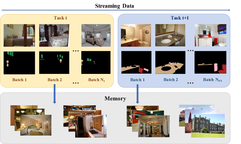
Figure 1. Overview of our online incremental semantic segmentation setting. Each incremental task adds images with annotations of new classes only for model adaptation, and a small set of data is saved for subsequent learning. We adopt the single-pass setting in which the data come as a stream of batches and can only be used once to update the model parameters. After each task, the model aims to segment all the semantic classes seen so far.

Semantic segmentation of visual scenes has recently witnessed tremendous progress thanks to pixel-level representation learning based on deep convolutional networks. Most existing works, however, assume a close-world setting, in which all the semantic classes of interest are given when a deep segmentation network is learned. This assumption, while simplifying the task formulation, can be restrictive in real-world applications, such as medical image analysis, robot sensing, and personalized mobile Apps (Li et al., 2019), where novel visual concepts need to be incorporated later on or continuously in deployment. To address this, a promising strategy is to incrementally learn semantic segmentation models (Michieli and Zanuttigh, 2019; Cermelli et al., 2020).

In this work, we focus on the problem of incrementally learning semantic segmentation model from a data stream (Aljundi et al., 2019a; Aljundi et al., 2019b). In contrast to the offline learning, our online learning task is bounded by the run-time and only allows single-pass through the data. Here we assume that, to reduce expensive labeling cost for semantic segmentation, we only receive annotations for the pixels of novel classes at their arrival as in (Cermelli et al., 2020). During training, we also assume that the system is able to save a subset of previously-seen training data as memory for rehearsal. This enables us to adapt the learned segmentation model to new label spaces with low annotation and training cost, and to cope with the scenarios that only limited legacy data resource can be stored due to privacy issue or data memory limitation. Fig. 1 illustrates the typical problem setting of this incremental semantic segmentation task. We note that most prior attempts on the incremental learning for semantic segmentation either adopt the offline learning setting without considering memory, or only focus on domain-specific tasks (Ozdemir et al., 2018; Tasar et al., 2019; Cermelli et al., 2020). By contrast, we aim to address the online incremental semantic segmentation with limited memory, which is more practical for many real-world scenarios.

There are several challenges in this online class incremental semantic segmentation problem given limited memory resource. First, continuous learning of novel visual concepts typically involves the so-called stability-plasticity dilemma, in which a model needs to quickly learn new concepts and meanwhile overcome catastrophic forgetting on learned visual knowledge (Rebuffi et al., 2017). In addition, the segmentation models have to cope with background concept drift as the background class changes due to the introduction of novel semantic classes, which further increases the difficulty of fast model adaption. Moreover, there also exists severe class-imbalanced problem due to varying co-occurrence of semantic classes in the data stream and small-sized memory.

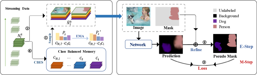
Figure 2. Overview of our framework. Each incremental step begins with a new training batch $\mathcal{N}_{t}^{k}$. Our method first samples a batch with the same size as the new batch from a class-balancing memory with a class probability $P_{s}$, which is dynamically updated at every step according to the prediction confidence of each class. The sampled batch is combined with the incoming data to build the training batch. We then update our model based on the EM learning framework: We fill in the missing annotations using confident predictions of the trained model, which produces the pseudo-masks for the training batch at E-step. At M-step, we train the model by optimizing the composite loss between the model predictions and the pseudo masks with cosine normalization. At the end of this incremental step, we use class-balanced exemplar selection to update the memory.

Our goal is to tackle all three aforementioned challenges in the online incremental learning of segmentation, aiming to achieve high learning efficiency with robustness towards catastrophic forgetting and concept drift. To this end, we propose a novel rehearsal-based deep learning strategy for building a segmentation network in an incremental manner. Our key idea is to train a deep network by utilizing incoming data batches at each incremental step with a dynamic sampling policy, which concentrates on informative samples from previous steps. This allows us to alleviate the catastrophic forgetting problem with low training cost. In addition, to improve the data efficiency and overcome the background drift, we introduce a re-labeling strategy in each incremental step, which fills in the missing annotations and updates the background class using confident predictions of the trained model. Furthermore, we integrate two class-balancing strategies, the cosine normalization and class-balanced exemplar selection, into the network training in each step to cope with unbalanced data.

Formally, we develop a unified learning approach that integrates the above strategies into an Expectation-Maximization (EM) based learning framework. Our method starts with a deep network trained on a set of base categories, and sequentially learns novel visual classes over incremental steps. In each step, our EM learning iterates through three stages: a) sampling a small set of training data, b) filling in missing labels of pixels, and c) updating the segmentation network using the dataset with mixed true and pseudo labels. After the parameter update, we adopt a class-balanced reservoir sampling strategy to update the exemplar set in the memory, which is then used for the next incremental step.

We evaluate our model on two challenging benchmarks, including PASCAL VOC 2012 and ADE20K datasets. Our empirical results and ablation study show that the proposed model achieves superior performance over prior incremental approaches, demonstrating the efficacy of our method. To summarize, the main contributions of our work are three-fold:

• We introduce a new online incremental learning problem for semantic segmentation, and our approach achieves the state-of-the-art results on two challenging benchmarks.

• We develop a unified EM framework that integrates a re-labeling step and a rehearsal-based training with dynamic sampling, promoting fast adaptation to novel classes and better alleviating catastrophic forgetting.

• To cope with imbalanced data in the online setting, we introduce cosine normalization and class-balanced reservoir sampling for incremental training of the segmentation networks.

2. Related Work

Semantic Segmentation

Recent research has made great progress in semantic segmentation based on deep convolutional network (Long et al., 2015; Ronneberger et al., 2015; Zhao et al., 2017; Chen et al., 2018). However, existing literature typically assumes that the semantic classes of interest and their annotated data are given in advance, which may not be feasible in practical open-world scenarios. To address this limitation, several recent works start to explore the problem of class-incremental semantic segmentation (Ozdemir et al., 2018; Cermelli et al., 2020; Michieli and Zanuttigh, 2019; Tasar et al., 2019). In particular, ILT (Michieli and Zanuttigh, 2019) uses annotations of both novel and old classes for each incremental task and adopts knowledge distillation to alleviate forgetting. MiB (Cermelli et al., 2020) revises the cross-entropy loss and knowledge distillation loss (Hinton et al., 2015) for solving forgetting and the bias caused by the background shift problem. Notably, MiB introduces a more natural setting requiring only the pixel annotations of novel classes, which is also adopted by our work.

It is worth noting that most existing approaches focus on tackling the incremental semantic segmentation with no memory of historical training data and in an offline manner (Michieli and Zanuttigh, 2019; Cermelli et al., 2020). The only exception is the work CoRiSeg (Ozdemir et al., 2018) for 3D medical image segmentation, which mainly addresses catastrophic forgetting with a distillation-based learning strategy on memory. In detail, it adopts a confidence-based strategy to select stored exemplars for rehearsal in the future. In this work, we also consider the more practical setting as in most of incremental classification works (Rebuffi et al., 2017; Wu et al., 2019; Yan et al., 2021) that provides a limited storage for past data. Nevertheless, our work do not focus on the offline training for each incremental task, and aims to continuously learn the segmentation model from a non-stationary data stream in an online manner. This enables many applications deployed on mobile devices to fast learn new concepts.

Class Incremental Learning

Class incremental learning aims to learn novel concepts continuously. There are mainly three kinds of methods in literature to solve the class incremental learning, which are regularization-based methods, distillation-based methods and structure-based methods. Regularization-based methods (Kirkpatrick et al., 2017; Zenke et al., 2017) penalizes the change of learned parameters which are important for previously observed classes. Distillation-based methods (Castro et al., 2018; Rebuffi et al., 2017; Wu et al., 2019; Douillard et al., 2020) retains learned knowledge via preserving the network output on the saved exemplars with knowledge distillation. Structured-based methods(Rajasegaran et al., 2019; Yan et al., 2021; Abati et al., 2020) separates parameters learned at different steps from each other to avoid undesirable overlapping in representations. For the online incremental learning setting, most existing methods rely on the rehearsal strategy and focus on better utilization of the memory. Specifically, AGEM (Chaudhry et al., 2019a), which is an efficient version of GEM (Lopez-Paz and Ranzato, 2017), projects the gradients computed on the new data to the direction that cannot increase the loss on the data sampled from memory. MIR (Aljundi et al., 2019a) proposes a sampling strategy selecting the maximally interfered data from memory to be learned with new data. GSS (Aljundi et al., 2019b) focuses on the construction of memory, which aims at maximizing the sample diversity based on their gradient directions. CBRS (Chrysakis and Moens, 2020) develops an class-balancing sampling strategy to deal with class-imbalanced stream of images. However, CBRS is designed for image classification and cannot be directly applied to semantic segmentation, which typically has instances from multiple classes in each image. In this work, we propose a new class-balancing strategy to handle this problem.

Re-labeling Strategy

Re-labeling, also known as self-training (Yarowsky, 1995; Papandreou et al., 2015; Hung et al., 2018), is a strategy to learn from partially labeled or unlabeled data. It takes the most probable predictions on unlabeled data as pseudo labels for subsequent model training. In this work, we incorporate the idea of re-labeling into a unified EM framework in order to accommodate the background concept drift and fill in missing labels of pixels in incoming data.

3. Our approach

In this section, we introduce our online incremental learning strategy for semantic segmentation, which aims to continuously learn novel visual concepts for pixel-wise semantic labeling of images. In particular, given a sequence of semantic classes, we consider the problem of building a segmentation model in multiple incremental tasks, each of which expands semantic label space with new arriving classes and needs to update the model with only limited data memory of previous tasks. In this limited-memory setting, our goal is to achieve efficient adaptation of the segmentation model without catastrophic forgetting of previously learned semantic classes.

To this end, we develop an Expectation-Maximization (EM) framework for incrementally learning a deep segmentation network. Our EM learning method incorporates a re-labeling strategy for augmenting annotations and an efficient rehearsal-based model adaptation with dynamic data sampling within a single framework. In addition, we introduce a robust training procedure for adapting the segmentation model based on cosine normalization and class-balanced memory. Such an integrated framework enables us to cope with the challenges of stability-plasticity dilemma, background concept drift and class-imbalance simultaneously in a principled manner. Below we start with an introduction of our problem setting in Sec. 3.1, followed by a formal description of our model architecture in Sec. 3.2. Then we present our EM-based incremental learning approach in Sec. 3.3. Finally, we show our class-balancing strategies in Sec. 3.4.

3.1. Problem Setup

The online incremental learning of semantic segmentation typically starts from a segmentation model $\mathcal{S}_{0}$, which is trained on a base task $\mathcal{T}_{0}=\{\mathcal{D}^{tr}_{0},\mathcal{Y}_{0}\}$ where $\mathcal{D}^{tr}_{0}$ is the training dataset, and $\mathcal{Y}_{0}$ are the base semantic classes. We denote the background class of $\mathcal{T}_{0}$ as $U_{0}$, which includes all the irrelevant classes not in $\mathcal{Y}_{0}$, and $\tilde{\mathcal{Y}}_{0}=\mathcal{Y}_{0}\cup\{U_{0}\}$ are the categories including background class at the initial task. The initial training set $\mathcal{D}^{tr}_{0}=\{(\mathbf{x}^{0}_{i},\mathbf{y}^{0}_{i})\}_{i=1}^{|\mathcal{D}^{tr}_{0}|}$, where $\mathbf{x}_{i}^{0}\in\mathbb{R}^{H\times W\times 3}$ and $\mathbf{y}_{i}^{0}\in\tilde{\mathcal{Y}}_{0}^{H\times W}$ are the $i$-th image and its fully-labeled annotation, respectively.

During the incremental learning stage, the initial segmentation model receives a stream of new semantic class groups $\{\mathcal{C}_{t}\}_{t\geq 1}$ and their corresponding training data $\{\mathcal{D}^{tr}_{t}\}_{t\geq 1}$ where $t$ indicates incremental steps. In each incremental step $t$, the training data also comes as a stream of mini-batches $\mathcal{N}^{k}_{t}\subset\mathcal{D}^{tr}_{t}$ where $k=1,\cdots,K$ and K is the number of min-batches. As in (Aljundi et al., 2019a; Chaudhry et al., 2018), our online learning setting only allows the model to perform one-step parameter update using the incoming batch $\mathcal{N}^{k}_{t}$. Here we assume that only pixels from the novel classes are labeled, which may be caused by lacking previous labeling expertise and/or limited annotation budget. Specifically, the incoming training data $\mathcal{N}^{k}_{t}$ has a form of $\{(\mathbf{x}^{t}_{i},\mathbf{y}^{t}_{i},\mathcal{R}_{i}^{t})\}_{i=1}^{|\mathcal{N}^{k}_{t}|}$ at step $t$, in which $\mathbf{y}^{t}_{i}$ is the partial annotation, and $\mathcal{R}^{t}_{i}$ is derived from $\mathbf{y}^{t}_{i}$ and indicates the labeled region in the image $\mathbf{x}^{t}_{i}$. For each pixel $j\in\mathcal{R}^{t}_{i}$, we have its label $\mathbf{y}^{t}_{i,j}\in\mathcal{C}_{t}$ and otherwise $\mathbf{y}^{t}_{i,j}$ is unlabeled.

Moreover, we assume a small set of exemplars $\mathcal{M}_{t}$ from previous steps can be stored in an external memory, and the allowable size of the memory is up to $\mathcal{B}_{\mathcal{M}}$. Typically, samples are drawn from memory, concatenated with the incoming batch and then used for training the segmentation model $\mathcal{S}_{t}$. Our goal is to learn an updated segmentation model $\mathcal{S}_{t}$ to incorporate the novel semantic classes in $\mathcal{C}_{t}$, and to achieve strong performance on a test data $\mathcal{D}^{ts}_{t}$. Below we refer to the model learning at each incremental step as a task. We note that $\mathcal{D}^{ts}_{t}$ includes all the semantic classes up to the $t$-th incremental step, denoted as $\mathcal{Y}_{t}=\mathcal{Y}_{0}\cup\left(\cup_{\tau=1}^{t}\mathcal{C}_{\tau}\right)$, and the corresponding background class $U_{t}$.

Algorithm 1 The Method Overview.

Initialize: Model $\mathcal{S}_{0}$; Memory $\mathcal{M}=\emptyset$

for $(\mathbf{x}_{i},\mathbf{y}_{i},\mathcal{R}_{i})\in\mathcal{D}^{tr}_{0}$ do

     CBES($\mathcal{M}$, $\mathbf{x}_{i}$, $\mathbf{y}_{i}$, $\mathcal{R}_{i}$)

end for

for $t=1,2,3...$ do

     while Batch $\mathcal{N}^{k}_{t}$ comes do

         $\tilde{\mathcal{N}}^{k}_{t}=\mathcal{N}_{t}^{k}$

         for $j=1,2,3...,|\mathcal{N}_{t}^{k}|$ do

              Sample the class $c_{k}$ according to $P_{s}(c)$ (Eq. 5)

              Denote $D_{s}\!=\!\{(\mathbf{x}_{l},\mathbf{y}_{l},\mathcal{R}_{l})\in\mathcal{M}_{t}|\,\exists j\in\mathcal{R}_{l},\,\mathbf{y}_{l,j}=c_{k}\}$

              Uniformly sample $(\mathbf{x}_{i},\mathbf{y}_{i},\mathcal{R}_{i})$ from $D_{s}$

              $\tilde{\mathcal{N}}^{k}_{t}=\tilde{\mathcal{N}}^{k}_{t}\cup\{\mathbf{x}_{i},\mathbf{y}_{i},\mathcal{R}_{i})\}$

         end for

         Refine label $\mathbf{y}_{i}$ in batch $\tilde{\mathcal{N}}_{t}^{k}$ by relabeling (Eq. 6)

         Update model $\mathcal{S}$ with the loss $\mathcal{L}$ (Eq. 7)

         Update class sampling probability $P_{s}(c)$ (Eq. 5)

         $\mathcal{M}^{k+1}_{t}\leftarrow\mathcal{M}^{k}_{t}$ // Update memory

         for $(\mathbf{x}_{i},\mathbf{y}_{i},\mathcal{R}_{i})\in\mathcal{N}^{k}_{t}$ do

              $\mathcal{M}^{k+1}_{t}$$=$$\text{CBES}(\mathcal{M}^{k+1}_{t},\mathbf{x}_{i},\mathbf{y}_{i},\mathcal{R}_{i})$

         end for

     end while

     $\mathcal{M}_{t+1}^{1}=\mathcal{M}_{t}^{k+1}$

end for

Algorithm 2 Class-balanced Exemplar Selection(CBES).

Input: Memory $\mathcal{M}_{t}$, data $(\mathbf{x}_{i},\mathbf{y}_{i},\mathcal{R}_{i})$

Category Set $Y_{i}=\text{Unique}(\mathbf{y}_{i})-\{U_{t}\}$

$c_{\text{min}}=\arg\min_{c\in Y_{i}}|\mathcal{M}^{c}_{t}|$

if  $|\mathcal{M}^{c_{\text{min}}}_{t}|<\mathcal{B}_{\mathcal{M}}/|\mathcal{Y}_{t}|$ or $|\mathcal{M}_{t}|<\mathcal{B}_{\mathcal{M}}$ then

     if  $|\mathcal{M}_{t}|==\mathcal{B}_{\mathcal{M}}$ then

         $c_{\text{max}}=\arg\max_{c\in\mathcal{Y}_{t}}|\mathcal{M}^{c}_{t}|$

         Randomly remove an image from $\mathcal{M}^{c_{\text{max}}}_{t}$

     end if

     Add $(\mathbf{x}_{i},\mathbf{y}_{i},\mathcal{R}_{i})$ into the memory $\mathcal{M}^{c_{\text{min}}}_{t}$

else

     for $c$ in $Y_{i}$ do

         $m_{c}$ $\leftarrow$ the number of saved images of class $c$

         $n_{c}$ $\leftarrow$ the number of seen images of class $c$

         Sample $p\sim Uniform(0,1)$

         if $p\leq m_{c}/n_{c}$ then

              Randomly remove an image from $\mathcal{M}^{c}_{t}$

              Add $(\mathbf{x}_{i},\mathbf{y}_{i},\mathcal{R}_{i})$ into $\mathcal{M}^{c}_{t}$

              Break

         end if

     end for

end if

3.2. Model Architecture

At each incremental step $t$, we assume a typical semantic segmentation network architecture, which consists of an encoder-decoder backbone network $\mathcal{F}_{t}$ extracting a dense feature map and a convolution head $\mathcal{H}_{t}$ that produces the segmentation score map. Concretely, given the image $\mathbf{x}_{i}$, the segmentation network first computes the convolutional feature map $\mathbf{F}_{i}\in\mathbb{R}^{H\times W\times D}$ using the backbone network, where $D$ is the number of channels. $\mathbf{F}_{i}$ is then fed into the $1\times 1$ convolution head $\mathcal{H}_{t}$, which has a form of linear classifier at each pixel location. Denote the parameters of the backbone network as $\mathbf{W}$, and the parameters of head as $\mathbf{\Psi}\in\mathbb{R}^{D\times(|\mathcal{Y}_{t}|+1)}$, our network generates its output $\mathbf{\hat{y}}_{i}$ as follows,

(1) $$\mathbf{F}_{i}=\mathcal{F}_{t}(\mathbf{x}_{i};\mathbf{W}),$$

(2) $$p(\mathbf{\hat{y}}_{i}|\mathbf{x}_{i})=\text{\small{Softmax}}(\mathcal{H}_{t}(\mathbf{F}_{i}))=\prod_{j\in\Omega_{i}}p(\mathbf{\hat{y}}_{ij}|\mathbf{F}_{ij};\mathbf{\Psi})$$

where $\Omega_{i}$ represents the 2D image plane and $\mathbf{F}_{ij}\in\mathbb{R}^{D}$ for the pixel $j$. Note that our method is agnostic to specific network designs.

3.3. Incremental Learning with EM

We now develop an EM learning framework to efficiently train the model $\mathcal{S}_{t}$ with a limited memory $\mathcal{M}_{t}$ in an online fashion. To tackle the stability-plasticity dilemma, our strategy integrates dynamic sampling and pixel relabeling, which enables us to efficiently re-use the training data for fast model adaptation and cope with background drift caused by the partial annotation.

Specifically, we formulate the online learning at each step as a problem of learning with latent variables and develop a stochastic EM algorithm to iteratively update the model parameters. In each step $t$, our learning procedure sequentially takes incoming mini-batch $\mathcal{N}_{t}^{k}$ and updates the model (denoted as $\mathcal{S}^{k}_{t}$) as well as the memory (denoted as $\mathcal{M}_{t}^{k}$). For each mini-batch, our EM algorithm iterates through three stages: 1) dynamic sampling of training data; 2) an E-step that relabels pixels with missing or background annotations, and 3) an M-step that updates the model parameters with one step of SGD. Below we denote the model parameter at min-batch $k$ in step $t$ as $\bm{\theta}^{k}_{t}=\{\mathbf{W}_{t}^{k},\mathbf{\Psi}_{t}^{k}\}$ and describe the details of the three stages in each EM iteration. A complete overview of our algorithm is shown in Algorithm 1.

Dynamic sampling

We first use a rehearsal strategy (Chaudhry et al., 2019b) to retrieve a sample of data from the memory, which has the same size as $\mathcal{N}_{t}^{k}$, and add them into the current mini-batch to build the training batch $\tilde{\mathcal{N}}_{t}^{k}$ for the subsequent EM update. Our goal is to achieve efficient model update that learns the new classes and also to retain old ones. To this end, we develop a dynamic sampling strategy to select informative samples from the memory.

Specifically, we devise a category-level sampling strategy that attempts to balance the training samples from the novel classes to be learned and the old ones prone to model forgetting. To achieve this, our method maintains a class sampling probability $P_{s}(c)$ for $\forall c\in\mathcal{Y}_{t}$, which will be described below. In order to sample a training image, we first sample a class label $c$ according to $P_{s}$, and then uniformly sample an image $\mathbf{x}_{i}$ that has pixels labeled with $c$. Such a sampling process allows the model to visit the data of certain classes more frequently and to improve the learning of those classes.

Our key design is to dynamically update the class probability $P_{s}$ according to the prediction confidence in the outputs of current model $\mathcal{S}^{k}_{t}$. To this end, we first compute an estimate of class confidences, denoted as $\{E(c),c\in\mathcal{Y}_{t}\}$, at every iteration of EM. Concretely, we use a moving average to collect the statistics from batches $\tilde{\mathcal{N}}_{t}^{k}$ as follows,

(3) $$E(c) =\mu E_{{old}}(c)+(1-\mu)E_{mb}(c),\quad$$

(4) $$E_{mb}(c) =\underset{{i\in\tilde{\mathcal{N}}^{k}_{t},\mathbf{{y}}_{i,j}=c}}{\text{Mean}}\{p(\mathbf{\hat{y}}_{i,j}=c|\mathbf{x}_{i};\bm{\theta}_{t}^{k-1})\}$$

where $E_{old}$ and $E_{mb}$ denotes the confidence estimate from last step and current mini-batch, respectively. Here $\mu$ is the momentum coefficient, and $\bm{\theta}_{t}^{k-1}$ is the model parameters after the update of last step. At the beginning of a new task $t$, we initialize $E(c)$ as $0$ for classes in $\mathcal{C}_{t}$.

Given the class confidences, we define the sampling probability $P_{s}$ with a Gibbs distribution, which assigns higher sampling probability to the classes with lower confidence:

(5) $$P_{s}(c)=\frac{e^{-\eta E(c)}}{\sum_{j=1}^{|\mathcal{Y}_{t}|}e^{-\eta E(j)}}\quad\forall c\in\mathcal{Y}_{t}$$

where $\eta$ is the hyperparameter to control the peakiness of the distribution.

E-step

In E-step, we tackle the problem of background concept drift due to the expansion of semantic label space $\mathcal{Y}_{t}$, and exploit the unlabeled regions in the training data of incremental steps for model adaption. To this end, we treat the labels of the background pixels in $\{\mathcal{D}^{tr}_{0}\}$ and the unlabeled pixels in $\{\mathcal{D}^{tr}_{t}\}_{t\geq 1}$ as hidden variables, and use the current model to infer their posterior distribution given the images and semantic annotations. We then use the posterior to fill in the missing annotations for the subsequent model learning in the M-step. By augmenting the training data with those pseudo labels, we aim to further improve the training efficiency and alleviate the problem of inconsistent background annotation.

Specifically, given a training pair $(\mathbf{x}^{\tau}_{i},\mathbf{y}^{\tau}_{i},\mathcal{R}_{i}^{\tau})\in\tilde{\mathcal{N}}_{t}^{k}$, we first compute an approximate posterior of the latent part of $\mathbf{y}^{\tau}_{i}$. Here $\tau\in\{0,\cdots,t\}$ indicates the incremental step it comes from. Denote the region with latent labels as $\bar{\mathcal{R}}_{i}^{\tau}$, the posterior of its $j$-th pixel can be estimated as $p(\mathbf{\hat{y}}_{i,j}|\mathbf{x}^{\tau}_{i};\bm{\theta}_{t}^{k-1})$ based on the current network. We then generate pseudo labels for those pixels by choosing the most likely label predictions as follows,

(6) $$\mathbf{{y}}^{\tau}_{i,j}=\underset{\mathbf{\hat{y}}_{i,j}\in\mathcal{\tilde{Y}}_{t}-\mathcal{C}_{\tau}}{\arg\max}p(\mathbf{\hat{y}}_{i,j}|\mathbf{x}^{\tau}_{i};\bm{\theta}_{t}^{k-1}),\quad j\in\bar{\mathcal{R}}^{i}_{\tau}$$

where $\mathcal{C}_{\tau}$ is the class group from step $\tau$. To filter out unreliable estimation, we only keep the pseudo labels of those pixels with confidence higher than a threshold $\delta$, i.e., $p(\mathbf{{y}}^{\tau}_{i,j}|\mathbf{x}^{\tau}_{i};\bm{\theta}_{t}^{k-1})>\delta$. We adopt this hard EM to update our model in the next stage.

M-step

Our M-step employs the mini-batch training data with augmented annotations to update the model parameters. In order to fully utilize the image annotations, we propose a composite loss consisting of two loss terms as follows,

(7) $$\mathcal{L}=-\sum_{i=1}^{|\tilde{\mathcal{N}}^{k}_{t}|}\left(\sum_{j=1}^{|\mathbf{{y}}^{\tau}_{i}|}\log p(\mathbf{{y}}^{\tau}_{i,j}|\mathbf{x}_{i}^{\tau};\bm{\theta}_{t}^{k})+\gamma\sum_{j=1}^{|\bar{\mathcal{R}}^{\tau}_{i}|}\log\sum_{z\in\tilde{\mathcal{Y}}_{t}\backslash\mathcal{C}_{\tau}}p(z|\mathbf{x}_{i}^{\tau};\bm{\theta}_{t}^{k})\right)$$

where $p(\cdot)$ is defined as in Equation (2) and $\gamma$ is a weighting coefficient. The first term is the standard cross-entropy loss on every pixel with real annotation or pseudo labels, while the second term penalizes the model on classifying the unlabeled pixels at step $\tau$ into label space $\mathcal{C}_{\tau}$, which encourages the labeling consistent with the partial groundtruth annotations.

3.4. Class Balancing Strategies

The online incremental learning of semantic segmentation typically has to face severe class imbalance in each step, which is caused by the limited mini-batch size and the data sampling. To address this issue, we introduce two strategies into the training of the segmentation network, which are detailed below.

Cosine Normalization

The model output at each pixel $j$ is represented as a probability vector $p(\mathbf{\hat{y}}_{ij}|\mathbf{F}_{ij};\mathbf{\Psi}^{k}_{t})$ with dimension $|\tilde{\mathcal{Y}}_{t}|$. Here the $m$-th element of the probability is defined as follows

(8) $$p(\mathbf{\hat{y}}^{m}_{ij}|\mathbf{F}_{ij};\mathbf{\Psi}^{k}_{t})=\frac{e^{\tau d(\mathbf{u}_{m},\mathbf{F}_{ij})}}{\sum_{c=1}^{|\tilde{\mathcal{Y}}_{t}|}e^{\tau d(\mathbf{u}_{c},\mathbf{F}_{ij})}}$$

where $\tau$ is the temperature used to control the sharpness of the softmax distribution, $\mathbf{u}_{m}\in\mathbb{R}^{D}$ is the m-th column of classifier weight $\mathbf{\Psi}^{k}_{t}$, and $d$ denotes the cosine distance. This enables us to alleviate the influence of biased norm due to class imbalance and produces more balanced scores across categories. It is worth noting that we are the first to adopt cosine normalization in the online class incremental learning problem, even though it has been used in other problems (Luo et al., 2018; Qi et al., 2018; Zhang et al., 2021).

Class-balanced Exemplar Selection

We then extend the class-balanced reservoir sampling (CBRS) (Chrysakis and Moens, 2020) to the incremental learning of semantic segmentation by taking into account the multiple classes in each image. Specifically, at the step $t$, we represent the memory for class $c$ as $\mathcal{M}_{t}^{c}=\{(\mathbf{x}_{i},\mathbf{y}_{i},\mathcal{R}_{i})|c\in\text{Unique}(\mathbf{y}_{i})\backslash\{U_{t}\}\}$. Here we ignore the mini-batch index $k$ for notation clarity. We build a class-balanced memory by maximizing the minimum size of $\mathcal{M}_{t}^{c}$, denoted as $\mathcal{M}_{t}^{c_{\text{min}}}$. Concretely, we save an image with the class $c_{\text{min}}$ into the memory if $|\mathcal{M}_{t}|<\mathcal{B}_{\mathcal{M}}$ or $\mathcal{M}_{t}^{c_{\text{min}}}$ is below the average size, i.e., $\mathcal{M}^{c_{\text{min}}}_{t}$ is smaller than $\mathcal{B}_{\mathcal{M}}/|\mathcal{Y}_{t}|$. Otherwise, we perform reservoir sampling for all the classes in $\mathbf{y}^{t}_{i}$ until an image is selected. Algorithm 2 describes the details of exemplar selection strategy.

4. Experiments

We evaluate our method on two online incremental learning benchmarks of semantic segmentation, which are built on the PASCAL VOC 2012 (Everingham et al., 2015) and ADE20K (Zhou et al., 2017) datasets, respectively. Below we first introduce our experimental setup in Sec. 4.1, followed by reporting our results and analysis on the PASCAL VOC 2012 benchmark in Sec. 4.2 and ADE20K in Sec. 4.3. Finally, we conduct an ablation study on the ADE20K dataset to analyze the contribution of our method components in Sec. 4.4.

4.1. Experiment Setup

We now describe the setup of our experimental evaluation from three aspects, including the learning protocol of deep segmentation networks, baseline methods for comparison and evaluation metrics.

Table 1. Mean IoU on the Pascal-VOC 2012 dataset for different incremental semantic segmentation splits. $*$ means the original method does not use an exemplar set and we apply the method on both incoming data and memory. The experiments are conducted under memory size $\mathcal{B}_{\mathcal{M}}=$100.

Methods	19-1						15-5						15-1
	Disjoint			Overlapped			Disjoint			Overlapped			Disjoint			Overlapped
	0-19	20	all	0-19	20	all	0-15	16-20	all	0-15	16-20	all	0-15	16-20	all	0-15	16-20	all
ER (Chaudhry et al., 2019b)	$71.04$	$23.36$	$68.77$	$71.02$	$15.96$	$68.39$	$65.20$	$28.94$	$56.57$	$65.37$	$27.84$	$56.44$	$66.6$	$24.98$	$56.69$	$68.64$	$15.37$	$55.95$
LwF.MC* (Rebuffi et al., 2017)	$72.65$	$27.56$	$70.51$	$72.12$	$24.46$	$69.85$	$69.89$	$36.55$	$61.95$	$71.85$	$36.26$	$63.38$	$68.68$	$30.81$	$59.66$	$69.73$	$30.19$	$60.32$
iCaRL (Rebuffi et al., 2017)	$58.81$	$8.73$	$56.44$	$60.38$	$7.63$	$57.87$	$60.06$	$19.71$	$50.45$	$59.39$	$24.97$	$51.19$	$61.48$	$3.23$	$47.61$	$63.78$	$7.35$	$50.35$
AGEM (Chaudhry et al., 2018)	$71.44$	$10.17$	$68.52$	$72.19$	$9.11$	$69.19$	$64.09$	$16.83$	$52.83$	$65.74$	$16.91$	$54.12$	$66.90$	$19.67$	$55.66$	$65.83$	$20.18$	$54.96$
MIR (Aljundi et al., 2019a)	$68.01$	$17.57$	$65.61$	$67.80$	$13.68$	$65.22$	$64.57$	$29.00$	$56.10$	$64.31$	$28.28$	$55.73$	$64.46$	$3.36$	$52.41$	$67.94$	$4.67$	$52.87$
MiB* (Cermelli et al., 2020)	$68.01$	$27.69$	$69.92$	$71.97$	$21.89$	$69.59$	$69.62$	$34.87$	$61.35$	$70.25$	$32.77$	$61.33$	$69.37$	$29.1$	$59.78$	$69.45$	$29.45$	$59.92$
CoRiSeg (Ozdemir et al., 2018)	$72.19$	$24.10$	$69.90$	$72.90$	$23.16$	$70.53$	$70.49$	$37.43$	$62.62$	$73.93$	$44.37$	$66.89$	$70.73$	$13.35$	$57.07$	$72.56$	$13.32$	$58.45$
Ours	$\bm{73.43}$	$\bm{39.10}$	$\bm{71.80}$	$\bm{73.76}$	$\bm{43.42}$	$\bm{72.32}$	$\bm{73.45}$	$\bm{47.89}$	$\bm{67.36}$	$\bm{75.56}$	$\bm{49.89}$	$\bm{69.45}$	$\bm{73.88}$	$\bm{37.15}$	$\bm{65.14}$	$\bm{75.77}$	$\bm{40.34}$	$\bm{67.33}$

Table 2. The performance of various methods with the fixed memory size $\mathcal{B}_{\mathcal{M}}\in\{20,50,100\}$, respectively. The experiments are conducted on the 15-1 disjoint split of PASCAL VOC 2012 dataset. $*$ means the original method does not use an exemplar set and we apply the method on both incoming data and memory

Methods	$\mathcal{B}_{\mathcal{M}}=20$		$\mathcal{B}_{\mathcal{M}}=50$		$\mathcal{B}_{\mathcal{M}}=100$
	imIoU	Final mIoU	imIoU	Final mIoU	imIoU	Final mIoU
ER (Chaudhry et al., 2019b)	$44.75$	$34.57$	$55.30$	$49.45$	$61.70$	$56.69$
LwF.MC* (Rebuffi et al., 2017)	$54.46$	$45.91$	$60.20$	$53.25$	$63.74$	$59.66$
iCaRL (Rebuffi et al., 2017)	$37.93$	$30.43$	$49.07$	$42.74$	$52.96$	$47.61$
AGEM (Chaudhry et al., 2018)	$50.84$	$43.89$	$52.80$	$46.98$	$54.15$	$51.01$
MIR (Aljundi et al., 2019a)	$47.07$	$37.46$	$54.83$	$47.14$	$61.81$	$52.41$
MiB* (Cermelli et al., 2020)	$56.98$	$48.90$	$61.93$	$54.34$	$64.41$	$59.78$
CoRiSeg (Ozdemir et al., 2018)	$54.50$	$45.42$	$60.73$	$52.06$	$64.59$	$57.07$
Ours	$\bm{64.64}$	$\bm{60.49}$	$\bm{65.57}$	$\bm{60.14}$	$\bm{68.06}$	$\bm{65.14}$

Online class-incremental Learning Protocol

To evaluate the performance of online incremental learning methods on fast adaptation and catastrophic forgetting, we adopt the following training protocol. Following the dataset split proposed in (Cermelli et al., 2020), we start from an initial model trained on a set of base classes and divide the remaining classes into different groups, which defines the incremental tasks to be learned sequentially. The word ”online” means data are coming in streaming form, i.e., each data batch can be seen only once. In addition, it is allowed to save limited history data in a memory buffer of fixed size.

Comparison Methods

To demonstrate the efficacy of our framework, we choose a set of typical incremental learning methods as our comparisons. Experience replay (ER) (Chaudhry et al., 2019b) is used as a basic continual learning strategy. LWF (Li and Hoiem, 2017) and ICARL (Rebuffi et al., 2017) are two widely adopted methods designed for the offline class-incremental classification. AGEM (Chaudhry et al., 2019a) and MIR (Aljundi et al., 2019a) are the methods for the online class-incremental classification. MIB (Cermelli et al., 2020) and CoRiSeg (Ozdemir et al., 2018) are two offline incremental learning methods for semantic segmentation but only the latter considers utilizing memory data.

Evaluation Metrics

We evaluate the model performance at the end of each incremental task. For each task, we use the mean of class-wise intersection over union (mIoU) as our metric, which includes the background class at each task. In addition, we take the incremental mean IoU (imIoU), which is computed as the average of the mIoU over different tasks, to measure the overall performance of the model over time.

Table 3. Mean IoU on the ADE20K dataset for different class incremental learning scenarios. $*$ means the original method does not use an exemplar set and we apply the method on both incoming data and memory.

Methods	100-50			100-10							50-50
	0-100	101-150	all	0-100	100-110	110-120	120-130	130-140	140-150	all	0-50	51-100	101-150	all
ER (Chaudhry et al., 2019b)	$33.02$	$2.71$	$22.98$	$32.59$	$3.48$	$4.17$	$0.01$	$\bm{1.61}$	$0.08$	$22.42$	$31.70$	$7.57$	$3.22$	$14.28$
LwF.MC* (Rebuffi et al., 2017)	$34.71$	$3.69$	$24.44$	$33.09$	$4.65$	$4.14$	$0.13$	$1.60$	$\bm{0.20}$	$22.84$	$34.99$	$9.07$	$4.14$	$16.19$
iCaRL (Rebuffi et al., 2017)	$21.63$	$0.00$	$14.46$	$22.77$	$0.00$	$0.00$	$0.00$	$0.00$	$0.01$	$15.22$	$28.13$	$0.00$	$0.00$	$9.50$
AGEM (Chaudhry et al., 2018)	$32.68$	$0.05$	$21.88$	$31.50$	$0.20$	$1.35$	$0.00$	$0.14$	$0.00$	$21.18$	$31.15$	$2.16$	$0.00$	$11.23$
MIR (Aljundi et al., 2019a)	$35.61$	$0.00$	$23.82$	$35.31$	$0.00$	$0.00$	$0.00$	$0.00$	$0.00$	$23.62$	$37.18$	$0.91$	$0.00$	$12.86$
MiB* (Cermelli et al., 2020)	$34.01$	$3.22$	$23.81$	$32.11$	$\bm{5.12}$	$3.71$	$0.01$	$1.41$	$0.13$	$22.17$	$33.55$	$8.61$	$3.58$	$15.37$
CoRiSeg (Ozdemir et al., 2018)	$36.58$	$0.36$	$24.58$	$32.41$	$0.00$	$0.21$	$0.00$	$0.00$	$0.00$	$21.69$	$40.20$	$1.25$	$0.31$	$14.10$
Ours	$\bm{36.80}$	$\bm{5.33}$	$\bm{26.38}$	$\bm{36.66}$	$4.83$	$\bm{12.87}$	$\bm{1.25}$	$0.42$	$0.06$	$\bm{25.81}$	$34.44$	$\bm{15.22}$	$\bm{7.15}$	$\bm{19.04}$

4.2. PASCAL VOC 2012

Dataset

The PASCAL VOC 2012 dataset (Everingham et al., 2015) consists of 10582 images in the training split and 1449 images in the validation split with a total of 21 different classes, including a background class given by the dataset. We use the validation split as our test set as the original test set is not publicly available. Following MiB(Cermelli et al., 2020), we also evaluate our method on both disjoint and overlapped setup where disjoint setup means that the images of each task is disjoint, and overlapped means there exist overlapped images between tasks. Moreover, we test our method on three different splits on both disjoint and overlapped setups. We begin with a model trained on 15 foreground classes, and the novel classes come incrementally in two streaming patterns, including 5 classes added at once (15-5) and sequentially, 1 at a time (15-1). Besides, we also start from a model trained on 19 foreground classes and one class is added at once (19-1). For the evaluation, we build a test set by taking all the images that contains known classes from the validation split.

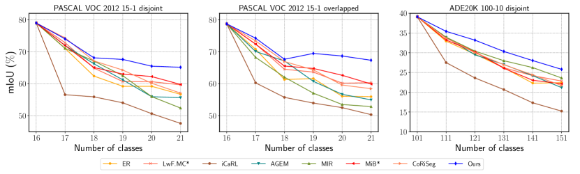
Figure 3. The mIoU of various methods with the Deeplab-v3 at different incremental tasks. The left two figures are the experiments on the VOC 2012 benchmark and the right two figures are on the ADE20K benchmark.

Implementation Details

We conduct our experiments based on DeepLab-v3 (Chen et al., 2017) with the ResNet101 (He et al., 2016) as the backbone. Following the protocol used in online incremental classification (Aljundi et al., 2019a), we hold out a validation set from the original training data to tune the hyper-parameters. The hyper-parameters of our method are $\delta=0.8,\gamma=0.5,\eta=1,\mu=0.9,\tau=12$. At the initial step, we start with the model pretrained on ImageNet and train the model for 60 epochs and adopt the SGD optimizer with batch size 24, momentum 0.9, weight decay 1e-4. The learning rate decays following the polynomial decay rule with power $0.9$. For the incremental stage, the incoming data comes as mini-batches with batch size 4. We concatenate the incoming batch with a same-sized batch(size=4) sampled from memory to form our mini-batch(size=8) for updating the model. We adopt SGD optimizer with learning rate 0.001 and momentum 0.9.

Quantitative Results

Tab. 1 summarizes the comparison results on PASCAL VOC 2012 benchmark. We can see that our method consistently outperforms other methods by a sizable margin at different incremental splits. Moreover, our method achieves better performance both on the old classes and the novel classes, which demonstrates that our strategy achieves faster adaptation on the streaming setting and is more robust towards catastrophic forgetting. Specifically, under the disjoint split of 15-1 setting, compared with the best baseline MiB*, we improve the final mIoU from 59.78 to 65.14(+5.36). We also plot the curves of mIoU at each incremental task for different methods in Fig. 3. We can see that the gap between our method and baselines increases over time.

Effects of Memory Size

We also conduct extensive experiments on the 15-1 disjoint split to explore the effect of memory size. The memory size(i.e. number of saved exemplars) ranges from 20 to 100, which is equivalently 1 to 5 exemplars per class on average, indicating different difficulty of the scenario. As shown in Tab. 2, our method consistently outperforms other methods on three memory sizes, for example, surpassing MiB by $7.66$ imIoU when $\mathcal{B}_{\mathcal{M}}=20$.

Table 4. Ablation Study on 50-50 split of ADE20K dataset. D.S.: dynamic sampling, C.R.: composite loss with relabeling, C.N.: cosine normalization, CBES: class-balanced exemplar selection.

Components				imIoU(%)
CBES	C.R.	C.N.	D.S.
✗	✗	✗	✗	$17.94$
✓	✗	✗	✗	$18.63$
✓	✓	✗	✗	$19.32$
✓	✓	✓	✗	$21.18$
✓	✓	✓	✓	$22.85$

4.3. ADE20K

Dataset

ADE20K (Zhou et al., 2017) is a large dataset for scene segmentation with 151 classes, including a background class given by the dataset. The dataset contains around 20K training, 2K validation and 3K test images. We evaluate our algorithm on the validation set as the test set has not been released. Like MiB (Cermelli et al., 2020), we adopt disjoint setup for ADE20K by spliting training images into disjoint image sets. Specifically, we begin with a model pretrained on 100 foreground classes and incrementally add the remaining 50 classes at once(100-50), or sequentially, 10 at a time(100-10). We also start from a model pretrained on 50 foreground classes and then add the remaining 100 classes sequentially, 50 at a time, denoted as 50-50. Besides, we also start from a model pretrained on 50 foreground classes and fifty classes are added sequentially, denoted as 50-50. The evaluation is consistent with PASCAL VOC 2012 benchmark, which builds the test set at task $t$ by selecting all images of known classes from validation set.

Implementation Details

At step 0, we start with the model pretrained on the ImageNet Dataset and train the model for 60 epochs and adopt the SGD optimizer with batch size 24, momentum 0.9, weight decay 1e-4. The learning rate starts with 1e-2 and decays following the polynomial decay rule with power 0.9. The hyper-parameters of our method are $\delta=0.8,\gamma=0.1,\eta=10,\mu=0.9,\tau=12$. For each incremental task, we start with constant learning rate 1e-3 , where the batch size is 8, weight decay 0.0001. Specifically, both the size of incoming mini-batch and the mini-batch retrieved from memory are 4. The other configurations are kept same as the ones in the experiments of PASCAL VOC 2012.

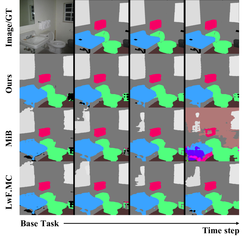
Figure 4. Visualization of our method, MiB and LwF.MC on ADE20K dataset. Top row shows the image and the change of actual ground truth over steps. The bottom three rows present the prediction of our method, MiB and LwF.MC at different tasks.

Quantitative Results

In Tab. 3, we compare our method with previous methods on ADE dataset. It is evident that our approach still consistently surpasses other methods with a large margin. Specifically, we outperform LWF.MC* with $2.85\%$ mIoU on the 50-50 split. As shown in Fig. 3, our method achieves more than 3$\%$ imIoU improvement at final task.

Qualitative Comparison

Fig. 4 shows visualization of the results of our method and two other methods. We can see that our method are more robust towards catastrophic forgetting compared with other methods.

4.4. Ablation Study

In Tab. 4, we conduct a series of ablation studies on ADE20K to evaluate the effect of our model components. We can see that each component plays a significant role in improving the final performance. In particular, class-balanced exemplar selection strategy outperforms the baseline ER by $0.69$ on imIoU. After adding the composite loss, the performance is improved from $18.63$ to $19.32$. Moreover, the cosine normalization further brings up the imIoU by $1.55$. In the end, the dynamic sampling strategy boosts the method from $21.18$ to $22.85(+\bm{1.67})$.

5. Conclusion

In this paper, we have introduced an online incremental learning problem for semantic segmentation, which is more practical for real-world applications. Our problem setting assume that a limited memory is available for model learning while the data comes in a streaming manner and the model updates its parameters only once for each incoming batch. To address this challenging problem, we develop a unified EM learning framework that integrates a re-labeling strategy for missing pixel annotations and an efficient rehearsal-based incremental learning step with dynamical sampling. Moreover, we also introduce cosine normalization and class-balanced memory to solve the class-imbalanced problem.Extensive experimental results on the PASCAL VOC 2012 and the ADE20K dataset demonstrate the advantages of our methods.

References

- (1)
- Abati et al. (2020) Davide Abati, Jakub Tomczak, Tijmen Blankevoort, Simone Calderara, Rita Cucchiara, and Babak Ehteshami Bejnordi. 2020. Conditional channel gated networks for task-aware continual learning. In Proceedings of the IEEE/CVF Conference on Computer Vision and Pattern Recognition(CVPR).
- Aljundi et al. (2019a) Rahaf Aljundi, Lucas Caccia, Eugene Belilovsky, Massimo Caccia, Min Lin, Laurent Charlin, and Tinne Tuytelaars. 2019a. Online continual learning with maximally interfered retrieval. In Advances in Neural Information Processing Systems(NeurIPS).
- Aljundi et al. (2019b) Rahaf Aljundi, Min Lin, Baptiste Goujaud, and Yoshua Bengio. 2019b. Gradient based sample selection for online continual learning. In Advances in Neural Information Processing Systems(NeurIPS).
- Castro et al. (2018) Francisco M Castro, Manuel J Marín-Jiménez, Nicolás Guil, Cordelia Schmid, and Karteek Alahari. 2018. End-to-end incremental learning. In Proceedings of the European Conference on Computer Vision (ECCV).
- Cermelli et al. (2020) Fabio Cermelli, Massimiliano Mancini, Samuel Rota Bulò, Elisa Ricci, and Barbara Caputo. 2020. Modeling the Background for Incremental Learning in Semantic Segmentation. In Proceedings of the IEEE Conference on Computer Vision and Pattern Recognition(CVPR).
- Chaudhry et al. (2018) Arslan Chaudhry, Marc’Aurelio Ranzato, Marcus Rohrbach, and Mohamed Elhoseiny. 2018. Efficient Lifelong Learning with A-GEM. In International Conference on Learning Representations(ICLR).
- Chaudhry et al. (2019a) Arslan Chaudhry, Marc’Aurelio Ranzato, Marcus Rohrbach, and Mohamed Elhoseiny. 2019a. Efficient Lifelong Learning with A-GEM. In International Conference on Learning Representations(ICLR).
- Chaudhry et al. (2019b) Arslan Chaudhry, Marcus Rohrbach, Mohamed Elhoseiny, Thalaiyasingam Ajanthan, Puneet K Dokania, Philip HS Torr, and Marc’Aurelio Ranzato. 2019b. On tiny episodic memories in continual learning. (2019).
- Chen et al. (2018) Liang-Chieh Chen, George Papandreou, Iasonas Kokkinos, Kevin Murphy, and Alan L. Yuille. 2018. DeepLab: Semantic Image Segmentation with Deep Convolutional Nets, Atrous Convolution, and Fully Connected CRFs. IEEE Transactions on Pattern Analysis and Machine Intelligence(TPAMI) (2018).
- Chen et al. (2017) Liang-Chieh Chen, George Papandreou, Florian Schroff, and Hartwig Adam. 2017. Rethinking atrous convolution for semantic image segmentation. arXiv preprint arXiv:1706.05587 (2017).
- Chrysakis and Moens (2020) Aristotelis Chrysakis and Marie-Francine Moens. 2020. Online Continual Learning from Imbalanced Data. In International Conference on Machine Learning(ICML).
- Douillard et al. (2020) Arthur Douillard, Matthieu Cord, Charles Ollion, Thomas Robert, and Eduardo Valle. 2020. Podnet: Pooled outputs distillation for small-tasks incremental learning. In Proceedings of the European Conference on Computer Vision (ECCV).
- Everingham et al. (2015) Mark Everingham, SM Ali Eslami, Luc Van Gool, Christopher KI Williams, John Winn, and Andrew Zisserman. 2015. The pascal visual object classes challenge: A retrospective. International Journal of Computer Vision(IJCV) (2015). http://host.robots.ox.ac.uk/pascal/VOC/voc2012.
- He et al. (2016) Kaiming He, Xiangyu Zhang, Shaoqing Ren, and Jian Sun. 2016. Deep residual learning for image recognition. In Proceedings of the IEEE Conference on Computer Vision and Pattern Recognition(CVPR).
- Hinton et al. (2015) Geoffrey Hinton, Oriol Vinyals, and Jeffrey Dean. 2015. Distilling the Knowledge in a Neural Network. In NeurIPS Deep Learning and Representation Learning Workshop.
- Hung et al. (2018) Wei-Chih Hung, Yi-Hsuan Tsai, Yan-Ting Liou, Yen-Yu Lin, and Ming-Hsuan Yang. 2018. Adversarial learning for semi-supervised semantic segmentation. In British Machine Vision Conference(BMVC).
- Kirkpatrick et al. (2017) James Kirkpatrick, Razvan Pascanu, Neil Rabinowitz, Joel Veness, Guillaume Desjardins, Andrei A Rusu, Kieran Milan, John Quan, Tiago Ramalho, Agnieszka Grabska-Barwinska, et al. 2017. Overcoming catastrophic forgetting in neural networks. Proceedings of the National Academy of Sciences(PNAS) (2017).
- Li et al. (2019) Dawei Li, Serafettin Tasci, Shalini Ghosh, Jingwen Zhu, Junting Zhang, and Larry P Heck. 2019. RILOD: near real-time incremental learning for object detection at the edge. In Proceedings of the 4th ACM/IEEE Symposium on Edge Computing(SEC).
- Li and Hoiem (2017) Zhizhong Li and Derek Hoiem. 2017. Learning without forgetting. IEEE Transactions on Pattern Analysis and Machine Intelligence(TPAMI) (2017).
- Long et al. (2015) Jonathan Long, Evan Shelhamer, and Trevor Darrell. 2015. Fully convolutional networks for semantic segmentation. In Proceedings of the IEEE Conference on Computer Vision and Pattern Recognition(CVPR).
- Lopez-Paz and Ranzato (2017) David Lopez-Paz and Marc’Aurelio Ranzato. 2017. Gradient episodic memory for continual learning. In Advances in Neural Information Processing Systems(NeurIPS).
- Luo et al. (2018) Chunjie Luo, Jianfeng Zhan, Xiaohe Xue, Lei Wang, Rui Ren, and Qiang Yang. 2018. Cosine normalization: Using cosine similarity instead of dot product in neural networks. In International Conference on Artificial Neural Networks.
- Michieli and Zanuttigh (2019) Umberto Michieli and Pietro Zanuttigh. 2019. Incremental learning techniques for semantic segmentation. In Proceedings of the IEEE International Conference on Computer Vision Workshops(ICCVW).
- Ozdemir et al. (2018) Firat Ozdemir, Philipp Fuernstahl, and Orcun Goksel. 2018. Learn the new, keep the old: Extending pretrained models with new anatomy and images. In International Conference on Medical Image Computing and Computer-Assisted Intervention(MICCAI).
- Papandreou et al. (2015) George Papandreou, Liang-Chieh Chen, Kevin P Murphy, and Alan L Yuille. 2015. Weakly-and semi-supervised learning of a deep convolutional network for semantic image segmentation. In Proceedings of the IEEE International Conference on Computer Vision(ICCV).
- Qi et al. (2018) Hang Qi, Matthew Brown, and David G Lowe. 2018. Low-shot learning with imprinted weights. In Proceedings of the IEEE conference on computer vision and pattern recognition(CVPR).
- Rajasegaran et al. (2019) Jathushan Rajasegaran, Munawar Hayat, Salman H. Khan, Fahad Shahbaz Khan, and Ling Shao. 2019. Random Path Selection for Continual Learning. In Advances in Neural Information Processing Systems(NeurIPS).
- Rebuffi et al. (2017) Sylvestre-Alvise Rebuffi, Alexander Kolesnikov, Georg Sperl, and Christoph H Lampert. 2017. icarl: Incremental classifier and representation learning. In Proceedings of the IEEE Conference on Computer Vision and Pattern Recognition(CVPR).
- Ronneberger et al. (2015) Olaf Ronneberger, Philipp Fischer, and Thomas Brox. 2015. U-net: Convolutional networks for biomedical image segmentation. In International Conference on Medical Image Computing and Computer-Assisted Intervention(MICCAI).
- Tasar et al. (2019) Onur Tasar, Yuliya Tarabalka, and Pierre Alliez. 2019. Incremental learning for semantic segmentation of large-scale remote sensing data. IEEE Journal of Selected Topics in Applied Earth Observations and Remote Sensing(JSTARS) (2019).
- Wu et al. (2019) Yue Wu, Yinpeng Chen, Lijuan Wang, Yuancheng Ye, Zicheng Liu, Yandong Guo, and Yun Fu. 2019. Large scale incremental learning. In Proceedings of the IEEE Conference on Computer Vision and Pattern Recognition(CVPR).
- Yan et al. (2021) Shipeng Yan, Jiangwei Xie, and Xuming He. 2021. DER: Dynamically Expandable Representation for Class Incremental Learning. In Proceedings of the IEEE/CVF Conference on Computer Vision and Pattern Recognition(CVPR).
- Yarowsky (1995) David Yarowsky. 1995. Unsupervised Word Sense Disambiguation Rivaling Supervised Methods. In 33rd Annual Meeting of the Association for Computational Linguistics(ACL).
- Zenke et al. (2017) Friedemann Zenke, Ben Poole, and Surya Ganguli. 2017. Continual learning through synaptic intelligence. In International Conference on Machine Learning(ICML).
- Zhang et al. (2021) Songyang Zhang, Zeming Li, Shipeng Yan, Xuming He, and Jian Sun. 2021. Distribution Alignment: A Unified Framework for Long-tail Visual Recognition. In Proceedings of the IEEE/CVF Conference on Computer Vision and Pattern Recognition(CVPR).
- Zhao et al. (2017) Hengshuang Zhao, Jianping Shi, Xiaojuan Qi, Xiaogang Wang, and Jiaya Jia. 2017. Pyramid scene parsing network. In Proceedings of the IEEE Conference on Computer Vision and Pattern Recognition(CVPR).
- Zhou et al. (2017) Bolei Zhou, Hang Zhao, Xavier Puig, Sanja Fidler, Adela Barriuso, and Antonio Torralba. 2017. Scene Parsing through ADE20K Dataset. In Proceedings of the IEEE Conference on Computer Vision and Pattern Recognition(CVPR).