Solution Enumeration by Optimality in Answer Set Programming

Abstract

Given a combinatorial search problem, it may be highly useful to enumerate its (all) solutions besides just finding one solution, or showing that none exists. The same can be stated about optimal solutions if an objective function is provided. This work goes beyond the bare enumeration of optimal solutions and addresses the computational task of solution enumeration by optimality (SEO). This task is studied in the context of Answer Set Programming (ASP) where (optimal) solutions of a problem are captured with the answer sets of a logic program encoding the problem. Existing answer-set solvers already support the enumeration of all (optimal) answer sets. However, in this work, we generalize the enumeration of optimal answer sets beyond strictly optimal ones, giving rise to the idea of answer set enumeration in the order of optimality (ASEO). This approach is applicable up to the best $k$ answer sets or in an unlimited setting, which amounts to a process of sorting answer sets based on the objective function. As the main contribution of this work, we present the first general algorithms for the aforementioned tasks of answer set enumeration. Moreover, we illustrate the potential use cases of ASEO. First, we study how efficiently access to the next-best solutions can be achieved in a number of optimization problems that have been formalized and solved in ASP. Second, we show that ASEO provides us with an effective sampling technique for Bayesian networks. This article is under consideration for acceptance in TPLP.

1 Introduction

In this paper, we address combinatorial problem solving where some solution components are combined to meet problem specific requirements. Such problems are frequent in computer science and computationally hard to solve since the number of solution candidates is usually exponential in the length of a problem instance [Karp (1972)]. Besides finding solutions for an instance, it is also possible to seek solutions that are optimal as defined by an objective function $f$ mapping solutions to numbers. In fact, combinatorial optimization problems described, e.g., by Korte and Vygen (?) tend to be computationally harder to solve, since the proof for optimality presumes the exclusion of yet better solutions. However, optimal solutions are not necessarily unique, suggesting the search and enumeration of all optimal solutions, e.g., for the sake of generating alternatives or better understanding the true nature of the objective function $f$. Besides enumeration, Murty (?) was interested in the ranking of solutions based on their cost, taking systematically into consideration sub-optimal solutions. While this idea is general by nature, it is applied to a specific problem where cost-optimal assignments are sought based on a cost matrix. If, in addition, a bound $k$ on the number of solutions is introduced, we arrive at the identification of the best $k$ solutions as in the case of the shortest path problem studied by Lawler (?).

In this work, we adopt the ideas discussed above and concentrate on the enumeration of optimal solutions but also take recursively into consideration sub-optimal but next-best solutions according to $f$. This gives rise to a systematic procedure that we coin as solution enumeration by optimality (SEO) which can also be understood as sorting solutions by their values obtained from the objective function. Since the underlying solution space is usually worst-case exponential, it is immediate that SEO poses computational challenges in general. For simplicity, we confine our attention to problems and solving paradigms yielding finite solution spaces in this work.

Besides tailoring native search algorithms, one viable way to solve combinatorial (optimization) problems is to describe their solutions in terms of constraints and to use existing solver technology for the search of actual solutions. To this end, well-known approaches are (maximum) Boolean satisfiability (SAT/MaxSAT) [Biere et al. (2009)], integer linear programming (ILP), constraint programming (CP) [Rossi et al. (2006)], and answer set programming (ASP) [Brewka et al. (2011)] with optimization [Simons et al. (2002), Brewka et al. (2003)]. While the number of solutions is generally unbounded in ILP, MaxSAT, CP, and ASP yield finite solution spaces in their standard use cases, hence enabling the exhaustive enumeration of all solutions in finite time.

As regards systematic solution enumeration, ASP offers somewhat better premises, since a typical ASP encoding aims at a one-to-one correspondence between solutions and answer sets. Gebser et al. (?) present dedicated algorithms for answer set enumeration (ASE) that are able to operate in polynomial space and to project answer sets with respect to a user-defined signature. Furthermore, in the presence of an objective function, the enumeration of optimal answer sets (ASO) is similarly feasible, once the respective optimum value of the objective function has been determined. In contrast, the enumeration features of contemporary SAT/MaxSAT solvers are quite limited although the algorithmic ideas are described by Gebser et al. (?). For this reason, we concentrate on ASP solvers that natively support solution enumeration (SE) and the enumeration of optimal solutions (SO) as discussed above, but not SEO in any systematic way.

Our main goal is to combine both answer set enumeration (ASE) and the enumeration of optimal answer sets (ASO) as the task of enumerating answer sets in the order of optimality as determined by an objective function $f$. In ASP, such functions are usually pseudo-Boolean expressions that assign integer weights to literals. The outcome, i.e., answer set enumeration by optimality (ASEO) realizes SEO under the view that answer sets bijectively capture the solutions of a problem being solved. In the sequel, we will explore ways to extend ASO procedures such that after enumerating all optimal solutions the search is continued to enumerate next-best solutions, and so on. Basically, this is achieved by performing ASO recursively but a careless implementation of this strategy may jeopardize the desired (polynomial) consumption of space.

When it comes to the enumeration of answer sets $S$ as guided by an objective function $f(S)$, we will explore two mainstream approaches. The first aims at enumerating all answer sets unless the enumeration procedure is interrupted by the user. The second presumes a parameter $k$ that gives the number of answer sets to be enumerated and, thereafter, the best $k$ answer sets $S$ are sought given $f(S)$. The latter approach opens up new possibilities for organizing ASEO when $k$ is small enough for storing intermediate solutions in memory. To realize these two approaches, we will deploy existing enumeration and optimization algorithms of Gebser et al. (?) and their implementations in the Clingo system. The main contributions of our work are:

1. The concept of answer set enumeration by optimality (ASEO) as a process where answer sets $S$ are produced in an order determined by an objective function $f(S)$.

2. Relating ASE, ASO, and ASEO from the perspective of computational complexity.

3. The development of basic algorithms that implement ASEO either in limited settings (the best $k$ answer sets) or without limitation (sorting answer sets subject to $f$).

4. An experimental evaluation of algorithms using ASP encodings of optimization problems.

5. Demonstrating the potential of ASEO in sampling guided by objective functions $f$.

It should be stressed that the main ideas of the paper can be generalized for other problem solving paradigms supporting optimization as long as the solution spaces are finite.

This paper is organized as follows. First, we briefly recall some concepts of answer set programming (ASP) and optimization in Section 2, and assess the computational complexity of solution enumeration by optimality (SEO) in the context of ASP (ASEO) in Section 3. Given these premises, we present our mixed algorithms for ASEO in Section 4. The efficiency of the novel ASEO algorithms is then studied in Section 5 by using optimization problems from ASP competitions as benchmarks. Yet further application is established in Section 6: it is shown and experimentally verified that our ASEO algorithms provide a potentially effective method for sampling and approximate inference on Bayesian networks. Section 7 concludes the paper.

2 Preliminaries

The basic syntax of answer set programming (ASP) [Brewka et al. (2011)] is based on rules

$${\and{h}_{1}}{\texttt{{|}}\,}\ldots{\texttt{{|}}\,}{\and{h}_{l}}\mathbin{\texttt{{:-}}\,}{\and{b}_{1}}{\texttt{{,}}\,}\ldots{\texttt{{,}}\,}{\and{b}_{n}}\texttt{{,}}\,{\texttt{{not}}\,\,\and{c}_{1}}{\texttt{{,}}\,}\ldots{\texttt{{,}}\,}{\texttt{{not}}\,\,\and{c}_{m}}\texttt{{.}}$$ (1)

where $\and{h}_{i}$:s, $\and{b}_{i}$:s, and $\and{c}_{i}$:s are atoms. A constraint is a rule (1) with an empty head ($l=0$). A logic program $P$ is a finite set of rules (1). The program $P$ is called normal if $l\leq 1$ holds for every rule (1) and disjunctive, otherwise. Given a set of atoms $A$, the reduct ${P}^{A}$ of $P$ with respect to $A$ contains a positive rule ${\and{h}_{1}}{\texttt{{|}}\,}\ldots{\texttt{{|}}\,}{\and{h}_{l}}\mathbin{\texttt{{:-}}\,}{\and{b}_{1}}{\texttt{{,}}\,}\ldots{\texttt{{,}}\,}{\and{b}_{n}}$ for each rule (1) of $P$ such that $l>0$ and no negated atom $\and{c}_{i}$ is in $A$. Given a logic program $P$, let $\mathrm{At}(P)$ be the signature of $P$, i.e., the set of atoms that occur in $P$. An answer set $A\subseteq\mathrm{At}(P)$ of $P$ (i) violates no constraint of $P$ and (ii) is a subset-minimal set closed under ${P}^{A}$, i.e., if ${\and{b}_{1}\in A}{,}\ldots{,}{\and{b}_{n}\in A}$ for some rule ${\and{h}_{1}}{\texttt{{|}}\,}\ldots{\texttt{{|}}\,}{\and{h}_{l}}\mathbin{\texttt{{:-}}\,}{\and{b}_{1}}{\texttt{{,}}\,}\ldots{\texttt{{,}}\,}{\and{b}_{n}}$ of ${P}^{A}$, then at least one $\and{h}_{i}$ is in $A$. Each program $P$ induces set of answer sets, denoted $\mathrm{AS}(P)$, usually capturing the solutions of a search problem encoded by $P$.

The syntax of ASP has been generalized in various ways as proposed, e.g., by Simons et al. (?), but many extensions can be translated back into rules of the form (1) using transformations of Bomanson et al. (?) and Alviano et al. (?). To cater for optimization problems within ASP, it is possible to introduce objective functions to identify optimal answer sets. For the purposes of this work, an objective function $f(A)$ is defined as a pseudo-Boolean expression

$${w_{1}\times l_{1}~{}}{+}\ldots{+}{~{}w_{n}\times l_{n}}=\sum_{i=1}^{n}(w_{i}\times l_{i})$$ (2)

where each $w_{i}$ is a non-negative integer weight and each $l_{i}$ is a literal, i.e., either an atom ‘$\and{a}$’ or its negation ‘$\texttt{{not}}\,\,\and{a}$’. If desired, negative weights can also be tolerated but typically reduced back to non-negative ones. Given an answer set $A\in\mathrm{AS}(P)$, the value $f(A)$ of (2) at $A$ is

$$\mathrm{eval}_{A}(\sum_{i=1}^{n}(w_{i}\times l_{i}))=\sum\{{w_{i}}\mid{1\leq i\leq n,~{}A\models l_{i}}\}$$ (3)

where $\models$ denotes the (standard) satisfaction of a literal $l_{i}$ in $A$: (i) $A\models\and{a}$ iff $\and{a}\in A$, and (ii) $A\models\texttt{{not}}\,\,\and{a}$ iff $\and{a}\not\in A$. An answer set $A\in\mathrm{AS}(P)$ is optimal (in the sense of minimization) if $f(A^{\prime})<f(A)$ for no $A^{\prime}\in\mathrm{AS}(P)$. Maximization can also be supported by transforming $f$ into $f^{\prime}$ suitable for minimization [Simons et al. (2002)]. Certain applications call for several objective functions $f_{i}$ (2) indexed by a priority level $1\leq i\leq p$. The resulting values (3) are interpreted lexicographically, i.e., $f_{1}(A)$ is the most important, then $f_{2}(A)$, etc. So, given an answer set (candidate) $A$, its (prioritized) objective value $f(A)$ is essentially a tuple $\langle{{f_{1}(A)}{,}\ldots{,}{f_{p}(A)}}\rangle$.

3 Complexity Landscape

In the following, we assume some familiarity with basic notions of computational complexity; see, e.g., the book of Papadimitriou (?) for an account. As regards decision problems, checking the existence of an answer set for a normal (resp. disjunctive) ground logic program given as input is $\mathbf{NP}$-complete (resp. $\Sigma^{\mathrm{p}}_{2}$-complete) as respectively shown by Marek and Truszczyński (?) and Eiter and Gottlob (?). However, the task of computing an optimal answer set $A$ for a normal logic program subject to an objective function $f$ forms an $\mathrm{FP}^{\mathbf{NP}}$-complete function problem as established by Simons et al. (?). This means that only polynomially many calls to an NP-oracle are required in the worst case. Indeed, the last call is typically the most demanding one since it excludes the existence of yet better answer sets. Once an optimal answer set $A$ has been determined, the respective optimum value $f(A)$ is naturally also known.

Let us then address the computational complexity of enumerating solutions in an order determined by an objective function $f$. Our first result concerns solution enumeration in general, i.e., the tasks SE, SO, and SEO, identified earlier. It is assumed that a search problem instance $P$ has some finite representation, ultimately encoded as a string, based on which solutions $S$ can be sought and enumerated, and the value $f(S)$ of the objective function $f$ is computable.

Proposition 1

Given a search problem instance $P$ and an objective function $f$, (i) the task SE is (constant-time) reducible to SO and SEO and (ii) the task SEO is not reducible to SE nor to SO in general.

Proof 3.1.

(i) The instance $P$ can be reduced to an instance $\langle{P,f}\rangle$ of SO and SEO by setting a constant value $f(S)=c$ for every solution $S$ of $P$. Then, both SO and SEO implement SE since the order of solutions is irrelevant and all solutions get enumerated in the end.

(ii) Suppose that the instance $\langle{P,f}\rangle$ of SEO were reducible to an instance $P^{\prime}$ of SE without an objective function. To enumerate the solutions of $P$, the instance $P^{\prime}$ must possess the same set of solutions. However, since there is no objective function for $P^{\prime}$ under SE, these solutions can be enumerated in any order, not necessarily compatible with $f$.

Quite similarly, suppose that the instance $\langle{P,f}\rangle$ of SEO is reducible to an instance $\langle{P^{\prime},f^{\prime}}\rangle$ of SO. Since the latter must yield all solutions to $P$, the instance $P^{\prime}$ must have the same solutions as $P$ and, in addition, each solution $S$ to $P^{\prime}$ must be optimal given $f^{\prime}$, i.e., $f^{\prime}(S)$ is constant. Thus, the (optimal) solutions to $P^{\prime}$ can be enumerated in any order, not necessarily compatible with $f$.

To conclude, reductions are not feasible in general, regardless of computational resources.

On the other hand, if only the enumeration of the best $k$ solutions is of interest, the respective enumeration task may become easier than SEO: fewer solutions have to be enumerated. For sufficiently small values of $k$, the task may be even easier than SO but harder than SO if $k$ exceeds the number of best solutions. However, the number of optimal solutions is not known in advance, which makes SEO an attractive option for the user. Typical answer set solvers perform SO with $k=1$ by default when optimizing answer sets. Next we concentrate on the enumeration of answer sets only and gather evidence that ASEO can be more demanding than ASE or ASO in general. One way to implement ASEO is to use ASO repeatedly as a subroutine and to exclude the solutions already enumerated by a constraint. It is established below that the intermediate instances of ASO remain equally hard enumeration problems in the worst case.

Theorem 3.2.

Given a normal logic program $P$ subject to an objective function $f$ of the form (2) and a non-negative integer lower bound $b$ for $f$, the task of computing the next-best answer set $A$ subject to $f(A)\geq b$ is $\mathrm{FP}^{\mathbf{NP}}$-complete.

Proof 3.3.

The bound $b$ and the objective function $f(A)$ for a candidate answer set $A$ can be incorporated by using a single weight rule $r$ [Simons et al. (2002)] that effectively expresses $f(A)\geq b$ and by translating that rule into normal rules [Bomanson et al. (2014)]. The translation $N(r)$ is feasible in polynomial time and $P\cup N(r)$ subject to $f$ is an (unbounded) instance of answer-set optimization and, thus, a member in $\mathrm{FP}^{\mathbf{NP}}$ as shown by Simons et al. (?). Hardness for $\mathrm{FP}^{\mathbf{NP}}$ is implied by the bound $b=0$ and the original (unbounded) complexity result of Simons et al. (?).

Proposition 1 does not cover the reducibility of an instance $\langle{P,f}\rangle$ of ASO with respect to ASE and ASEO. Interestingly, if the objective value $f(A)=b$ for a best answer set $A$ were known, reductions would become feasible. By expressing the condition $f(A)\leq b$ with a weight rule $r$ rewritten as a set $N(r)$ of normal rules (cf. the proof of Theorem 3.2), the instance $P\cup N(r)$ of ASE, or the instance $\langle{P\cup N(r),f}\rangle$ of ASEO, would capture the original ASO problem. The key observation is that such a bound $b$ on $f$ cannot be determined in general in polynomial time.

Proposition 3.4.

The problem ASO is not polytime reducible to ASE nor to ASEO unless $\mathbf{P}=\mathbf{coNP}$.

Proof 3.5.

Let $P$ be a normal program forming an instance of deciding if $\mathrm{AS}(P)=\emptyset$ or not. In general, this problem was shown $\mathbf{coNP}$-complete by Marek and Truszczyński (?). Let us construct a program $Q$ by introducing new atoms $\and{a}$ and $\and{b}$ as well as rules “$\and{a}\mathbin{\texttt{{:-}}\,}\texttt{{not}}\,\,\and{b}\texttt{{.}}$”, “$\and{b}\mathbin{\texttt{{:-}}\,}\texttt{{not}}\,\,\and{a}\texttt{{.}}$”, and the rules of $P$ conditioned by the atom $\and{b}$. Then $\{\and{a}\}\in\mathrm{AS}(Q)$ and, if $A\in\mathrm{AS}(P)$, then $A\cup\{\and{b}\}\in\mathrm{AS}(Q)$. By setting an objective function $f(A)=2\times\and{a}+1\times\and{b}$, the answer set $\{\and{a}\}$ is optimal only if answer sets of the latter kind do not exist. Towards our goal, let us assume that $R$ is the polytime reduction of $\langle{Q,f}\rangle$ into an ASE problem. We can check in polynomial time if $\{\and{a}\}\in\mathrm{AS}(R)$ (i.e., whether it should be enumerated by ASE), iff $\mathrm{AS}(P)=\emptyset$.

Similarly, let $\langle{R,g}\rangle$ be a polytime reduction of $\langle{Q,f}\rangle$ into an ASEO problem. Again, we can test if $\{a\}\in\mathrm{AS}(R)$ in polynomial time, giving rise to two cases. (i) If $\{\and{a}\}\not\in\mathrm{AS}(R)$, then $Q$ has answer sets of the form $A\cup\{\and{b}\}$, all to be enumerated by ASEO and equally admitted by $g$, i.e., $f(A\cup\{\and{b}\})=b$ is constant. Thus $\mathrm{AS}(P)\neq\emptyset$. (ii) If $\{\and{a}\}\in\mathrm{AS}(R)$, two subcases arise:

1. If $g(\{\and{a}\})$ is not minimal, then $R$ must have an answer set $B\neq\{\and{a}\}$ such that $g(B)<g(\{\and{a}\})$. Without loss of generality, assume that $g(B)$ is minimal. Then $B$ is to be enumerated by ASEO but also $\{a\}$, since ASEO will enumerate the inferior answer sets as well. Then both $B$ and $\{a\}$ should enumerated by ASO on the input $\langle{Q,f}\rangle$, a contradiction.

2. Thus $g(\{\and{a}\})$ is minimal and $\{\and{a}\}$ is to be enumerated by ASEO. Then it must be enumerated by ASO given $\langle{Q,f}\rangle$ excluding all other answer sets. Thus $\mathrm{AS}(P)=\emptyset$.

Thus we obtained a (hypothetical) polynomial-time test whether $\mathrm{AS}(P)=\emptyset$.

Proposition 3.6.

In the worst case, a (normal) logic program $P$ subject to an objective function $f$ may possess exponentially many answer sets $A$ with different objective values $f(A)$.

Proof 3.7.

For an illustration, let us consider a concrete normal program $P_{n}$ based on atoms ${\and{a}_{1}}{,}\ldots{,}{\and{a}_{n}}$ and ${\and{b}_{1}}{,}\ldots{,}{\and{b}_{n}}$ parameterized by $n$. The intended objective function $f({\and{a}_{1}}{,}\ldots{,}{\and{a}_{n}})=\sum_{i=1}^{n}2^{i-1}\times\and{a}_{i}$. Thus assignments to ${\and{a}_{1}}{,}\ldots{,}{\and{a}_{n}}$ encode distinct values in the range ${0}{,}\ldots{,}{2^{n}-1}$ in binary. Using complementary atoms $\overline{\and{a}}$ for the atoms $\and{a}$ involved, the rules of $P_{n}$ are for all $i={1}{,}\ldots{,}{n}$:

$\and{a}_{i}\mathbin{\texttt{{:-}}\,}\texttt{{not}}\,\,\overline{\and{a}}_{i}\texttt{{.}}$	$\overline{\and{a}}_{i}\mathbin{\texttt{{:-}}\,}\texttt{{not}}\,\,\and{a}_{i}\texttt{{.}}$	$\and{b}_{i}\mathbin{\texttt{{:-}}\,}\texttt{{not}}\,\,\overline{\and{b}}_{i}\texttt{{.}}$	$\overline{\and{b}}_{i}\mathbin{\texttt{{:-}}\,}\texttt{{not}}\,\,\and{b}_{i}\texttt{{.}}$
$\and{lt}_{i}\mathbin{\texttt{{:-}}\,}\overline{\and{a}}_{i}\texttt{{,}}\,\and{b}_{i}\texttt{{.}}$	$\and{lt}_{i}\mathbin{\texttt{{:-}}\,}\and{a}_{i}\texttt{{,}}\,\and{b}_{i}\texttt{{,}}\,\and{lt}_{(i+1)}\texttt{{,}}\,(i<n)\texttt{{.}}$		$\and{lt}_{i}\mathbin{\texttt{{:-}}\,}\overline{\and{a}}_{i}\texttt{{,}}\,\overline{\and{b}}_{i}\texttt{{,}}\,\and{lt}_{(i+1)}\texttt{{,}}\,(i<n)\texttt{{.}}$
$\mathbin{\texttt{{:-}}\,}\and{b}_{1}\texttt{{,}}\,\and{lt}_{2}\texttt{{.}}$	$\mathbin{\texttt{{:-}}\,}\overline{\and{b}}_{1}\texttt{{,}}\,\texttt{{not}}\,\,\and{lt}_{2}\texttt{{.}}$

The rules of $P_{n}$ serve the following purposes. The rules of the first line simply choose truth values for $\and{a}_{i}$:s and $\and{b}_{i}$:s. The rules in the second line check whether the value represented by $\and{a}_{i}$:s is lower than the value represented by $\and{b}_{i}$:s such that $\and{lt}_{i}$ takes bits ${i}{,}\ldots{,}{n}$ into account. Regarding constraints in the third line, they accept only one half of possible values for $\and{b}_{i}$:s given some fixed values of $\and{a}_{i}$:s. Thus $P_{n}$ has $2^{n-1}$ answer sets $A$ corresponding to each (fixed) assignment to the atoms ${\and{a}_{1}}{,}\ldots{,}{\and{a}_{n}}$ and, in total, $2^{n}\times 2^{n-1}=2^{2n-1}$ answer sets.

Given an answer set $A$ of $P_{n}$, the objective value $f(A)$ is $f({\and{a}_{1}}{,}\ldots{,}{\and{a}_{n}})=\sum_{i=1}^{n}2^{i-1}\times\and{a}_{i}$ based on the truth values of ${\and{a_{1}}}{,}\ldots{,}{\and{a}_{n}}$ in $A$. Given $P_{n}$ and $f$, any ASEO algorithm must enumerate all answer sets $A$ with value $f(A)=0$ first, all answer sets with value $f(A)=1$ next, and so on, until (finally) all answer sets with value $f(A)=2^{n}-1$ get enumerated. Each subtask in this sequence can be viewed as an ordinary ASO task yielding $2^{n-1}$ assignments for $\and{b}_{i}$:s and those assignments are different for each assignment of $\and{a}_{i}$:s. This is to prevent the learning of nogoods for systematically excluding certain values of $\and{b}_{i}$:s. In this way, $P_{n}$ maximally exercises the underlying enumeration procedure, although finding a single answer set is yet easy.

4 Algorithms for Answer Set Enumeration by Optimality

Propositions 1–3.6 support the view that ASEO can be strictly more demanding task than ASE and ASO. This, however, does not prevent us from using ASE and ASO as subroutines when realizing ASEO in practice. Therefore, we implement our ASEO algorithms on top of a state-of-the-art ASP solver Clingo [Gebser et al. (2008)] treated as a black box for running ASO and ASE subtasks for systematic answer set enumeration. Clingo implements an efficient search for answer sets, as witnessed by ASP competitions (see, e.g., the report of Calimeri et al. (?)), deploying conflict-driven nogood learning (CDNL) algorithms devised by Gebser et al. (?). However, sub-optimal answer sets cannot be readily enumerated, thus motivating the goals of our work. A way to implement ASEO is to use Clingo’s Python API that extends the functionality of the underlying solver. While the API enables quite straightforward implementation of ASEO algorithms detailed in the sequel, it excludes certain options available for native implementations.

We call our first approach to ASEO the naive algorithm. The algorithm simply enumerates all answer sets one by one with the help of Clingo API during which pairs $\langle{A,f(A)}\rangle$ of answer sets $A$ and the respective objective values $f(A)=\langle{{f_{1}(A)}{,}\ldots{,}{f_{p}(A)}}\rangle$ for priority levels are recorded for an input program $P$. Once the ordinary ASE task is completed, the pairs recorded are sorted lexicographically based on their objective values. Then the output consists of all answer sets of the program in the sorted order. While our naive algorithm for ASEO is easy to implement, its obvious weakness is its consumption of space. However, it may perform surprisingly well in cases where the number of answer sets is low. Therefore, it makes a reasonable baseline algorithm for our purposes as well as a basis for comparisons against more sophisticated algorithms.

Algorithm 1 Weight Enumeration

Input:	Program: $P$, Integer: $k$
	Objective functions: $(1,(l^{1}_{1},w^{1}_{1}),\dots,(l^{1}_{n_{1}},w^{1}_{n_{1}})),\dots,(p,(l^{p}_{1},w^{p}_{1}),\dots,(l^{p}_{n_{p}},w^{p}_{n_{p}})$
Output:	Sorted answer sets: $S$

1:  $S\leftarrow\{\}$;   $p^{\prime}\leftarrow p$;   $P^{\prime}\leftarrow P$

2:  while $p^{\prime}\geq 1$ do

3:     $A$ $\leftarrow$ ASP-Optimize($P^{\prime}$)

4:     if UNSAT($P^{\prime}$) and $p^{\prime}>1$ then

5:        if $|S|=0$ then

6:           return $S$

7:        end if

8:        $p^{\prime}\leftarrow p^{\prime}-1$;   $P^{\prime}\leftarrow P$

9:        for $i$ from $1$ to $p^{\prime}-1$ do

10:           $P^{\prime}\leftarrow P^{\prime}\cup\{\mathrm{EQ}_{i}(C[i])\}$

11:        end for

12:        $P^{\prime}\leftarrow P^{\prime}\cup\{\mathrm{GT}_{l}(C[p^{\prime}])\}$

13:     else

14:        $P^{\prime}\leftarrow P$;   $C\leftarrow[~{}]$

15:        for $i$ from $1$ to $p$ do

16:           $C[i]\leftarrow\mathrm{eval}_{A}(\sum_{j=1}^{n_{i}}(w_{j}^{i}\times l_{j}^{i}))$;   $P^{\prime}\leftarrow P^{\prime}\cup\{\mathrm{EQ}_{i}(C[i])\}$

17:        end for

18:        for $A^{\prime}\leftarrow$ ASP-Solve($P^{\prime}$) do

19:           $S\leftarrow S\cup\{A^{\prime}\}$

20:           if $|S|=k$ then

21:              return $S$

22:           end if

23:        end for

24:        $p^{\prime}\leftarrow p$;   $P^{\prime}\leftarrow P$

25:        for $i$ from $1$ to $p^{\prime}-1$ do

26:           $P^{\prime}\leftarrow P^{\prime}\cup\{\mathrm{EQ}_{i}(C[i])\}$

27:        end for

28:        $P^{\prime}\leftarrow P^{\prime}\cup\{\mathrm{GT}_{l}(C[p^{\prime}])\}$

29:     end if

30:  end while

31:  return $S$

In contrast with the naive algorithm, the ASEO task can be alternatively implemented without enumerating all answer sets first. Such a procedure is obtained by first (i) performing ASO followed by (ii) the introduction of constraints that exclude solutions enumerated so far. Finally, (iii) the ASO task is performed on increasingly constrained problem instances until the desired number of answer sets have been found. The constraints have to be introduced with extra care so that the (polynomial) space consumption of the underlying ASEO task is not jeopardized. Algorithm 1 is such a constraining algorithm that augments the input program $P$ between subsequent enumeration tasks. Once all currently optimal answer sets have been enumerated, it appends constraints that make subsequent answer sets strictly worse than those enumerated so far. We know by Theorem 3.2 that this does not necessarily make the remaining computational task any easier, i.e., the subsequent computation of next-best solutions can still be challenging. For a cost $C=\mathrm{eval}_{A}(\sum_{j=1}^{n_{i}}(w_{j}^{i}\times l_{j}^{i}))$ associated with an answer set $A$ and a priority level $1\leq i\leq p$, a rule-based constraint $\mathrm{GT}_{i}(C)$, mimicking the ASP core standard [Calimeri et al. (2020)], is:

$$\mathbin{\texttt{{:-}}\,}~{}\texttt{{\#sum\{}}{w^{i}_{1}~{}\texttt{{:}}~{}l^{i}_{1}}{\texttt{{;}}\,}\ldots{\texttt{{;}}\,}{w^{i}_{n_{i}}~{}\texttt{{:}}~{}l^{i}_{n_{i}}}\texttt{{\}}}~{}\texttt{{<=}}~{}C\texttt{{.}}$$ (4)

The objective value at the priority level $1\leq i\leq p$ is fixed with a similar constraint $\mathrm{EQ}_{i}(C)$:

$$\mathbin{\texttt{{:-}}\,}\texttt{{\#sum\{}}{w^{i}_{1}~{}\texttt{{:}}~{}l^{i}_{1}}{\texttt{{;}}\,}\ldots{\texttt{{;}}\,}{w^{i}_{n_{i}}~{}\texttt{{:}}~{}l^{i}_{n_{i}}}\texttt{{\}}}~{}\texttt{{!=}}~{}C\texttt{{.}}$$ (5)

The weight enumeration algorithm starts in Line 2 by discovering an optimal answer set $A$ using Clingo’s optimization algorithm. The call ASP-Optimize$(P^{\prime})$ returns an optimal answer set, if such an answer set $A$ exists. Lines 5–7 cover programs having no answer sets. Lines 14–23 calculate objective values ${f_{1}(A)}{,}\ldots{,}{f_{p}(A)}$ for priority levels and introduce constraints (5) to enumerate all equally good answer sets. Enumeration is done by Clingo’s answer set enumeration algorithm designed by Gebser et al. (?): it performs branch-and-bound search based on literals in the input program and conflicts that occur during the enumeration. In Line (18), the call ASP-Solve$(P^{\prime})$ receives all answer sets of $P^{\prime}$, one at a time. Once these get enumerated, Lines 24–29 deploy constraints (5) for levels $i={1}{}\ldots{}{p^{\prime}-1}$ and a constraint (4) for level $p^{\prime}$ to find next-best answer sets. Lines 4–12 are used to virtually relax all constraints in the augmented program $P^{\prime}$ so that next-best answer sets from the following priority level can be enumerated.

Example 4.8.

Consider an optimization program $P$ with three answer sets $A_{1}$, $A_{2}$, and $A_{3}$ with objective values $f(A_{1})=\langle{1,4,1}\rangle$, $f(A_{2})=\langle{1,4,7}\rangle$, and $f(A_{3})=\langle{1,7,4}\rangle$. Algorithm 1 starts by discovering the (only) optimal answer set $A_{1}$ and constrains the answer sets $A$ of $P$ by $f_{1}(A)=1$, $f_{2}(A)=4$, and $f_{3}(A)>1$. These make $A_{2}$ optimal and once found, the last is revised to $f_{3}(A)>7$. As a result, no answer sets exist, the constraints for $f_{2}$ and $f_{3}$ are superseded by $f_{2}(A)>4$. When $A_{3}$ is found, the constraints are revised to $f_{1}(A)=1$, $f_{2}(A)=7$, and $f_{3}(A)>4$. From this point onward, no answer sets are met, the level $p^{\prime}$ is decreased down to $1$, and Algorithm 1 terminates.

Few observations about Algorithm 1 are worthwhile. First, it is designed to find the best $k$ answer sets as determined by the given objective functions ${f_{1}}{,}\ldots{,}{f_{p}}$. If the full ASEO is rather desired, the parameter $k$ should be set to $\infty$, enforcing the algorithm to loop over all answer sets in an order compatible with ${f_{1}}{,}\ldots{,}{f_{p}}$. Second, the algorithm uses an (ordered) set $S$ as an intermediate storage for answer sets. Instead of storing found answer sets in $S$, an option is to process them immediately, e.g., by printing them for the user. This saves the space taken by $S$.

Proposition 4.9.

Algorithm 1 can be implemented so that it runs in space polynomial in $|\mathrm{At}(P)|$.

Proof 4.10.

The ASE and ASO tasks are feasible in polynomial space, see the CNDL-ENUM-ASP algorithm of Gebser et al. (?) for details. Using this algorithm via the Clingo API, Algorithm 1 is able to enumerate optimal as well as sub-optimal answer sets. Lines 4 and 12 therein relax constraints used to exclude optimal answer sets enumerated during previous solver calls by forgetting them and by adding tightened ones. Thus the size of $P$ does not increase indefinitely and Algorithm 1 operates in space comparable to CNDL-ENUM-ASP regardless the value of $k$.

Due to our black-box implementation, Algorithm 1 may suffer from restarts after enumerating all answer sets pertaining to a particular objective value. The underlying solver could benefit from previously learned conflicts and there is even further potential expected from keeping track of seen non-optimal answer sets that could be reused in subsequent runs. However, such functionalities call for a native enumeration algorithm and/or modifications to the underlying solver.

Algorithm 2 Smart Enumeration

Input:	Program: $P$, Integer: $k$
	Objective functions: $(1,(l^{1}_{1},w^{1}_{1}),\dots,(l^{1}_{n_{1}},w^{1}_{n_{1}})),\dots,(p,(l^{p}_{1},w^{p}_{1}),\dots,(l^{p}_{n_{p}},w^{p}_{n_{p}})$
Output:	Sorted answer sets: $S$

1:  $S\leftarrow[]$;   $t\leftarrow\langle{\infty,\ldots,\infty}\rangle$;   $L\leftarrow\{\}$;   $A\leftarrow\{\}$

2:  for $L$ $\leftarrow$ ASP-Enumerate($P$) do

3:     $C\leftarrow[]$

4:     for $i$ from $1$ to $p$ do

5:        $C[i]\leftarrow\mathrm{eval}_{L}(\sum_{j=1}^{n_{i}}(w_{j}^{i}\times l_{j}^{i}))$

6:     end for

7:     if $L$ is complete then

8:        $S\mathrm{.insert}(\langle{L^{+},C}\rangle)$

9:        if $|S|>k$ then

10:           $S\mathrm{.remove}(k+1)$

11:           $\langle{A,t}\rangle\leftarrow S[k]$

12:        end if

13:     else if $C>t$ then

14:        $P\leftarrow P\cup\{\mathbin{\texttt{{:-}}\,}L\texttt{{.}}\}$

15:     end if

16:  end for

17:  return $S$

Algorithm 2 realizes a window-based approach where answer sets are computed using an ASE process while keeping the best $k$ answer sets ${A_{1}}{,}\ldots{,}{A_{k}}$ in memory. In addition, the objective value $f(A_{k})$ of the $k$:th best answer set is used as a threshold $t$ to discard found (partial) answer sets that are worse than $A_{k}$ and thus not contributing to the top $k$ answer sets. Our implementation of Algorithm 2 relies much on Clingo API as it needs to keep track of assigned literals as well as to introduce new nogoods for excluding answer sets. As regards storing answer sets, the space requirement of Algorithm 2 is $k\times|\mathrm{At}(P)|$. If the underlying ASE algorithm were completely used a black box, the actual enumeration of answer sets is feasible in space polynomial in $|\mathrm{At}(P)|$, but for sufficiently large values of $k$, this is dominated by $k\times|\mathrm{At}(P)|$. However, since Algorithm 2 adds nogoods explicitly and for a different purpose than the underlying ASE algorithm, their number may become exponential in $|\mathrm{At}(P)|$ in contrast with Algorithm 1 (cf. Proposition 4.9). This issue can be best approached in terms of either native algorithms or an enhanced API that is able to keep track and manipulate nogoods used for different purposes.

The main loop of smart enumeration in Lines 2–16 start with a call to ASP-Enumerate$(P)$ that is based on the standard ASE algorithm of Gebser et al. (?). The call provides a new partial assignment $L$, i.e., a set of literals for the input program $P$. For each iteration of the loop, $L$ is extended by some chosen literal $l$ and further literals may be derived using propagation. The underlying enumeration algorithm is also responsible for backtracking if $L$ becomes inconsistent. Note that since $L$ is partial, (3) is revised to $\mathrm{eval}_{L}(\sum_{i=1}^{n}(w_{i}\times l_{i}))=\sum\{w_{i}\mid 1\leq i\leq n,l_{i}\in L\}$. If $L$ is complete (covers all of $\mathrm{At}(P)$), Lines 8–12 append the respective answer set $L^{+}=\{{\and{a}\in L}\mid{\and{a}\in\mathrm{At}(P)}\}$ and the corresponding cost(s) $C$ to the list $S$ of best $k$ solutions so far. Moreover, the threshold value $t$ for excluding future answer sets is updated. Line 8 implements insertion sort and places $\langle{L^{+},C}\rangle$ in the list $S$ based on its cost(s) $C$. However, if $L$ is not yet complete and its cost vector $f(L)$ is greater than the current threshold value $t$, the program $P$ can be extended by a nogood for excluding all supersets of $L$ as done in Lines 13–15. The algorithm terminates once the whole search space limited by the nogoods is exhausted.

Example 4.11.

Consider a single objective function $f$ as defined by $(l_{1},5)$, $(l_{2},1)$, $(l_{3},2)$, $(l_{4},2)$, $(l_{5},6)$ and all possible answer sets $A_{1}=\{l_{1},l_{2},l_{3}\}$, $A_{2}=\{l_{1},l_{3},l_{5}\}$, $A_{3}=\{l_{2},l_{3},l_{5}\}$, $A_{4}=\{l_{1},l_{2},l_{4}\}$, $A_{5}=\{l_{1},l_{4},l_{5}\}$ of a program $P$ for which the best $k=2$ answer sets are sought. Suppose that $f(A_{4})=8$ and $f(A_{3})=9$ are the currently known top $k=2$ answer sets which gives threshold $t=9$. If $L=\{l_{1}\}$ is the current partial answer set and the search heuristic picks $l_{5}$ as the next literal to branch on, we end up with $L^{\prime}=\{l_{1},l_{5}\}$ with cost $f(L^{\prime})=11$. Since $11>t$, any extensions of $L^{\prime}$ are eliminated by a nogood $\mathbin{\texttt{{:-}}\,}l_{1},l_{5}\texttt{{.}}$ Thus the underlying ASP solver will skip $A_{2}$ and $A_{5}$ altogether as it cannot construct the corresponding partial assignments anymore.

Algorithms 1 and 2 work quite differently. For the program $P_{n}$ from the proof of Proposition 3.6, there exist exponentially many answer sets while finding and enumerating optimal values is easy. Using Algorithm 1 on this problem instance is fast due to easy enumeration while Algorithm 2 slows down as it needs to find objective values among an exponential number of possibilities.

5 Benchmarking: Optimization Problems

Table 1: Experimental results for ASEO algorithms

Instance					Target Answer Sets $k$
Problem	#Instances	Naive	Alg	$10$	$100$	$10^{3}$	$10^{4}$	#TO
BayesianNL	$30$	$1800s$ $(30)$	Alg 1	$\boldsymbol{41s}$	$\boldsymbol{67s}$	$\boldsymbol{171s}$	$\boldsymbol{460s}$	$\boldsymbol{2}$
			Alg 2	$919s$	$991s$	$1083s$	$1379s$	$64$
MarkovNL	$30$	$1800s$ $(30)$	Alg 1	$\boldsymbol{185s}$	$\boldsymbol{311s}$	$\boldsymbol{757s}$	$\boldsymbol{1499s}$	$\boldsymbol{28}$
			Alg 2	$1800s$	$1800s$	$1800s$	$1800s$	$110$
Supertree	$35$	$1099s$ $(10)$	Alg 1	$457s$	$591s$	$696s$	$855s$	$32$
			Alg 2	$\boldsymbol{391s}$	$\boldsymbol{417s}$	$\boldsymbol{507s}$	$\boldsymbol{830s}$	$\boldsymbol{29}$
Connected	$20$	$301s$ $(0)$	Alg 1	$\boldsymbol{1613s}$	$1713s$	$1771s$	$1800s$	$73$
			Alg 2	$1685s$	$\boldsymbol{1684s}$	$\boldsymbol{1702s}$	$\boldsymbol{1760s}$	$\boldsymbol{72}$
MaxSAT	$10$	$1800s$ $(10)$	Alg 1	$\boldsymbol{21s}$	$\boldsymbol{721s}$	$\boldsymbol{902s}$	$\boldsymbol{919s}$	$\boldsymbol{14}$
			Alg 2	$1098s$	$1368s$	$1790s$	$1800s$	$32$
FastFood	$20$	$212s$ $(1)$	Alg 1	$\boldsymbol{1s}$	$\boldsymbol{1s}$	$\boldsymbol{7s}$	$500s$	$\boldsymbol{0}$
			Alg 2	$10s$	$9s$	$31s$	$\boldsymbol{185s}$	$1$
Hamilton	$45$	$46s$ $(0)$	Alg 1	$\boldsymbol{126s}$	$350s$	$797s$	$1243s$	$32$
			Alg 2	$187s$	$\boldsymbol{216s}$	$\boldsymbol{261s}$	$\boldsymbol{394s}$	$\boldsymbol{18}$

The performance of our ASEO algorithms is evaluated on several optimization problems adopted from ASP competitions, as reported by Calimeri et al. (?). The criterion for choosing problems was solvability by Clingo in a reasonable time. For each benchmark problem, the difficulty of instances increases and the numbers of answer sets are problem-specific. In the experiments, we measure runtime subject to a timeout of $1\,800\,s$. All experiments are conducted using an Intel(R) Xeon(R) CPU (E5-1650 v4 @ 3.60GHz), with 32GB RAM, and Ubuntu OS.

Table 1 collects the results obtained for optimization problems. The rows of the table detail runs on different problems while columns denote different runs of our algorithms. The second column shows average time for the naive algorithm as well as number of timeouts in parentheses. The last column shows the collective number of timeouts (#TO) for an enumeration algorithm. A single cell reports the average runtimes for all instances of the benchmark problem in question, and for Algorithms 1 and 2. For each target of enumeration, the better algorithm is indicated in boldface. The average runtimes suggest that the weight enumeration algorithm tends to perform better than smart enumeration. Even when smart enumeration gives faster results, the runtime of weight enumeration is not too far off. Average runtimes obtained for BayesianNL and MaxSAT highlight how much faster weight enumeration can be while Hamilton is the only benchmark with a reverse effect. Yet it is important to note that for certain benchmarks, namely Connected and Hamilton, the naive algorithm that enumerates all answer sets first works faster than others.

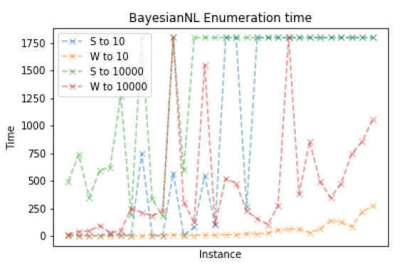
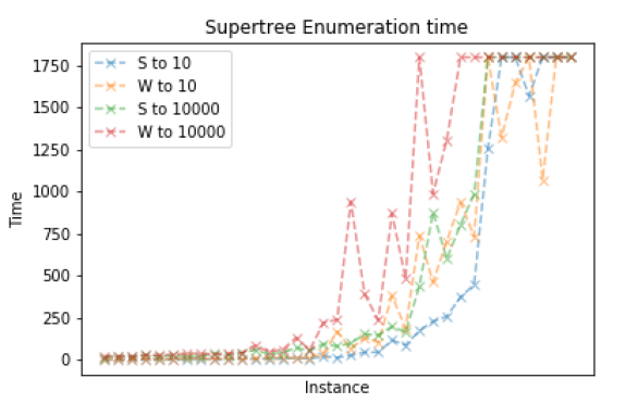
(a) Runtimes on BayesianNL	(b) Runtimes on Supertree

Figure 1: Cactus plots for selected experiments

Fig. 1 reflects how enumeration algorithms scale differently. Fig. 1(a) reveals that BayesianNL is relatively easy for weight enumeration (W). The switch from enumerating $10$ answer sets to $10^{4}$ answer sets seems to increase the runtime of weight enumeration somewhat linearly. Meanwhile, the performance of smart enumeration (S) algorithm degrades rabidly to the timeout. In the same vein, we observe from Fig. 1(b) that the two enumeration algorithms scale quite similarly in the Supertree benchmark problem. Their runtimes start to increase simultaneously but the increase is more drastic for weight enumeration than it is for smart enumeration, and the latter algorithm runs always slightly faster than the former. It is evident that the algorithms behave differently across the instances and relative to each other. Algorithm 1 works considerably better than others when finding an optimal objective value and enumerating optimal values is easy as, for example, in the case of the logic program introduced in the proof of Proposition 3.6. However, enumeration based algorithms work better when the number of answer sets is reasonably low such that they can be enumerated in comparable time. Algorithm 2 seems to perform especially well when the objective values ${f(A_{1})}{\leq}\ldots{\leq}{f(A_{k})}$ for the best $k$ answer sets ${A_{1}}{,}\ldots{,}{A_{k}}$ vary a lot and it is easier to locate the threshold value $t=f(A_{k})$ for ruling out worse answer sets.

To summarize the experiments reported in this section, Algorithm 1 (weight enumeration) works reasonably well for a majority of the problem instances. It seems to be able to discover next-best answer sets with ease similar to the previous ones and our best experimental results indicate linear increase in time with respect to the desired number of answer sets $k$. Meanwhile, Algorithm 2 (smart enumeration) does not perform as well on average and it fails on problem instances that are easy for weight enumeration. However, we are able to demonstrate that there exist problems for which the smart enumeration algorithm can be faster and thus beneficial.

6 Practical Application: Bayesian Sampling

Figure 2: ASEO-based approximation of probabilities

Table 2: Bayesian networks used in the experiments

Network Features					Algorithm Features
Network	Nodes	Arcs	Avg. Degree	$k$
Boe 92	23	36	3.13	$200$
Win-95	76	112	2.95	$500$
Andes	223	338	3.03	$2000$

For a practical application of ASEO, let us consider probabilistic inference in the context of Bayesian networks (BNs) with Boolean random variables and an approach similar to weighted model counting [Chavira and Darwiche (2008)]. The goal is to approximate queries by computing Maximum a Posteriori (MAP) assignments using an ASP encoding of the respective abduction problem devised by Beaver and Niemelä (?). The optimal solutions of the problem satisfy

$$c_{\mathrm{MAP}}=\operatorname*{arg\,max}_{C}\left(p(C|e)\right),$$ (6)

i.e., $c_{\mathrm{MAP}}$ is an assignment to random variables $C$ in a network $N$ that makes the observed evidence $e$ in $N$ most probable. Given a (Boolean) query variable $q$, the same ASP encoding and the ASEO algorithms proposed in this work can be used to enumerate assignments in a decreasing order of significance, i.e., starting from MAP assignments but continuing with next probable assignments, and so on. This leads to a goal directed sampling method as follows. Given a query $q$ and some evidence $e$, we find out the $k$ most probable assignments ${c_{1}}{,}\ldots{,}{c_{k}}$ (resp. ${d_{1}}{,}\ldots{,}{d_{k}}$) that satisfy $q$ (resp. $\neg q$) and are compatible with $e$. Thus, we obtain an estimate

$$P(q|e)\approx\frac{\sum_{i=1}^{k}P(q,c_{i}\mid e)}{\sum_{i=1}^{k}P(q,c_{i}\mid e)+\sum_{i=1}^{k}P(\neg q,d_{i}\mid e)}.$$ (7)

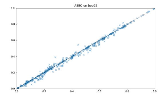
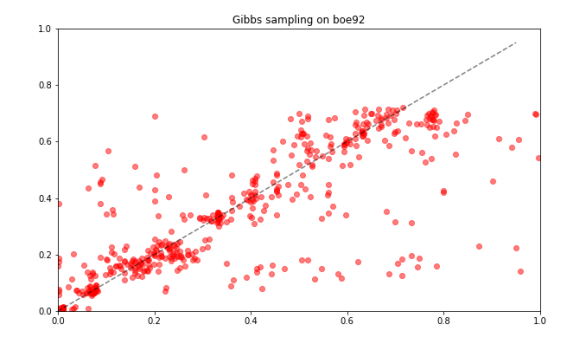
(a) ASEO on Boe 92	(b) Gibbs on Boe 92
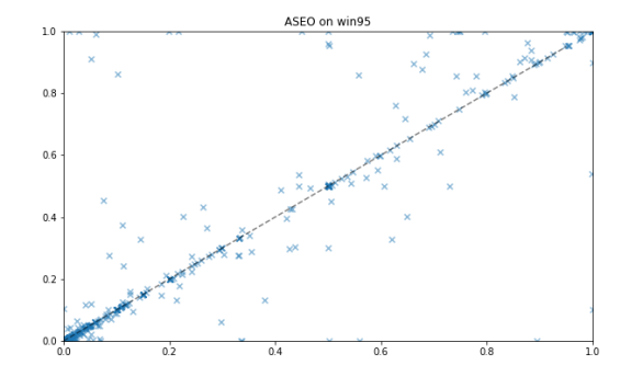
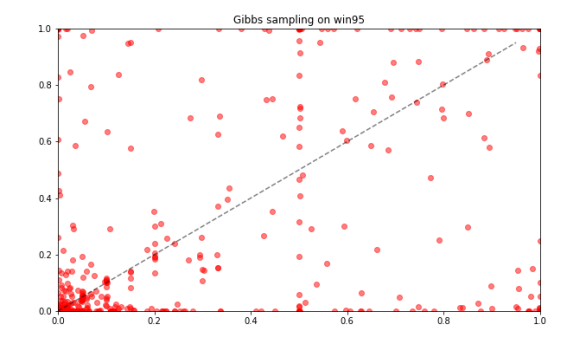
(c) ASEO on Win-95	(d) Gibbs on Win-95
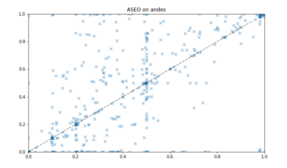
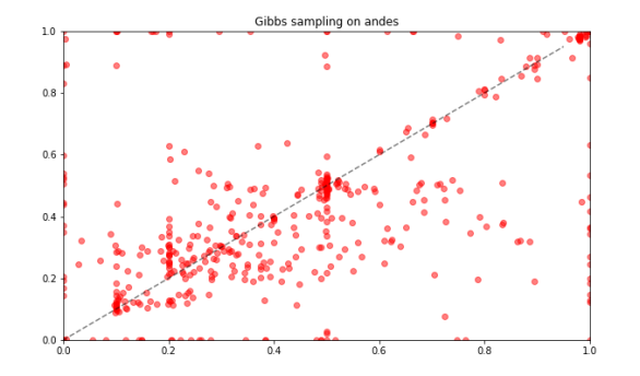
(e) ASEO on Andes	(f) Gibbs on Andes

Figure 3: Results of approximation algorithms compared to true probabilities in the networks

Figure 2 illustrates the full procedure for approximating the query $q$ given the evidence $e$. First, for the sake of fair comparison with other sampling methods, the network is simplified using d-separation following Geiger et al. (?). Second, the input network is transformed into an ASP encoding for solving the respective MAP problem. Then, based on the given evidence $e$, the query $q$, and its negation $\neg q$, up to $k$ most probable assignments are computed in order to approximate the probability $p(q|e)$ in the sense of (7). Then, we evaluate our ASEO-based sampling method using few publicly available BNs whose size varies from small to large (cf. Table 2). The experiments are conducted by randomly picking a query variable and a set of evidence variables that represent $1$ to $50\%$ of the variables in the network in total. In what follows, we compare our sampling results to those obtained with a well-known native algorithm, viz. Gibbs sampler as provided in the pyAgrum library of Gonzales et al. (?). In this implementation, the sampler stops by determining the convergence of the approximation with $\epsilon=0.01$.

Table 3: Measured errors of approximations

Average distance
Algorithm	Boe 92	Win-95	Andes
ASEO	$0.03$	$0.04$	$0.16$
Gibbs sampler	$0.07$	$0.11$	$0.15$
Maximum error
Algorithm	Boe 92	Win-95	Andes
ASEO	$0.11$	$0.98$	$0.99$
Gibbs sampler	$0.81$	$0.99$	$0.99$

In Fig. 3, the sampling results for the input networks are presented. To obtain the results we use Algorithm 1 to conduct ASEO where the choice of the enumeration algorithm was based on better overall performance. In each image, true probabilities are mapped on the $x$-axis while the respective estimates are represented on the $y$-axis. Hence, the closer to the diagonal points are, the better approximations have been obtained. When looking at distributions, we observe that the ASEO-based approximations tend to be better on smaller networks while this is no longer obvious for the largest network Andes. As far as we can see, this is due to the fact that with larger networks there exists increasing number of assignments with an equal objective value (i.e., the same probability) and individual assignments having very low probability values. As a consequence, we do not get a good overview of the distribution of probabilities and the probabilities are far from the expected true ones as for the Andes network.

Table 3 presents further qualitative results over approximations where distances to true probabilities are measured. The results of the table illustrate that ASEO-based sampling can be competitive even with known methods such as Gibbs sampler. However, when considering approximate reasoning task like Bayesian sampling, one should remember that there are highly optimized exact methods, such as that of Madsen and Jensen (?), to determine true probabilities fast.

7 Discussion and Conclusion

In this work, we address solution enumeration in the context of combinatorial optimization problems, the goal of which is to generate all optimal solutions to a given problem instance. As a novelty, we take also sub-optimal solutions into consideration and propose algorithms that are able to recursively enumerate next-best solutions until (i) all solutions or, alternatively, (ii) the best $k$ solutions have been enumerated. Such a procedure realizes our concept of solution enumeration by optimality (SEO). Besides screening the computational cost of SEO, we present dedicated SEO algorithms geared toward answer set programming (ASP) where solutions are captured with answer sets. The resulting ASEO algorithms are implemented in Python [Pajunen (2020)] using the API of the Clingo solver and are put to the test in experiments. These algorithms generalize the ASO reasoning mode of Clingo. Moreover, we mention that the computation of $k$ best solutions was considered in an experimental track of MaxSAT Evaluation run by Bacchus et al. (?), but the solutions enumerated were supposed to assign different values to literals involved in the objective function. Thus, such an enumeration differs from SEO up to $k$ solutions.

The experimental evaluation comprises of two parts. First, we evaluate our ASEO algorithms on a number of optimization problems that have been used in ASP competitions. The results indicate the feasibility of ASEO in practice, enabling the exploitation of next-best solutions when solving optimization problems. This is good news from the perspective of Theorem 3.2 which indicates that the remaining computational complexity does not necessarily decrease when excluding answer sets already enumerated. Second, we illustrate the potential of ASEO in approximating Bayesian inference. There is some resemblance to the approach of Chavira and Darwiche (?) based on weighted model counting. The difference is that the objective function derived from conditional probability tables guides the search toward the most relevant assignments for query evaluation. Ermon et al. (?) deploy optimization oracles for similar inference but in the presence of further constraints for uniformly distributing samples over the space of assignments. It is worth noting that Bayesian inference has been well studied and there are further good alternatives to ASEO. Our main objective is to demonstrate the new way of utilizing objective functions, effectively SEO, as means to reach the most significant solutions first.

As discussed in Section 4, our proof-of-concept implementations of ASEO are still sub-optimal as they are essentially based on successive calls to ASO/ASE algorithms via an API. This prevents, e.g., the direct exploitation of nogoods learned during the subsequent invocations of the underlying enumeration algorithm. This observation suggests an obvious goal for future work: a native implementation of an ASEO reasoning mode in some state-of-the-art answer-set solver. To this end, we hope that our results make this goal attractive for developers.

Acknowledgments.

The second author has been partially supported by the Academy of Finland projects ETAIROS (327352) and AI-ROT (335718).

References

- Alviano et al. (2015) Alviano, M., Faber, W., and Gebser, M. 2015. Rewriting recursive aggregates in answer set programming: back to monotonicity. Theory Pract. Log. Program. 15, 4-5, 559–573.
- Bacchus et al. (2020) Bacchus, F., Berg, J., Järvisalo, M., and Martins, R. 2020. MaxSAT evaluation. https://maxsat-evaluations.github.io/2020/topk.html.
- Beaver and Niemelä (1999) Beaver, H. and Niemelä, I. 1999. Finding MAPs for belief networks using rule-based constraint programming. Arpakannus.
- Biere et al. (2009) Biere, A., Heule, M., van Maaren, H., and Walsh, T. 2009. Handbook of Satisfiability. Frontiers in Artificial Intelligence and Applications, vol. 185. IOS Press.
- Bomanson et al. (2014) Bomanson, J., Gebser, M., and Janhunen, T. 2014. Improving the normalization of weight rules in answer set programs. In Proc. of JELIA’14. Springer, 166–180.
- Brewka et al. (2011) Brewka, G., Eiter, T., and Truszczyński, M. 2011. Answer set programming at a glance. Communications of the ACM 54, 12, 92–103.
- Brewka et al. (2003) Brewka, G., Niemelä, I., and Truszczynski, M. 2003. Answer set optimization. In Proc. of IJCAI’03. Vol. 3. Morgan Kaufmann, 867–872.
- Calimeri et al. (2020) Calimeri, F., Faber, W., Gebser, M., Ianni, G., Kaminski, R., Krennwallner, T., Leone, N., Maratea, M., Ricca, F., and Schaub, T. 2020. Asp-core-2 input language format. TPLP 20, 2, 294–309.
- Calimeri et al. (2016) Calimeri, F., Gebser, M., Maratea, M., and Ricca, F. 2016. Design and results of the fifth answer set programming competition. Artificial Intelligence 231, 151–181.
- Chavira and Darwiche (2008) Chavira, M. and Darwiche, A. 2008. On probabilistic inference by weighted model counting. Artif. Intell. 172, 6-7, 772–799.
- Eiter and Gottlob (1995) Eiter, T. and Gottlob, G. 1995. On the computational cost of disjunctive logic programming: Propositional case. Annals of Mathematics and Artificial Intelligence 15, 3–4, 289–323.
- Ermon et al. (2013) Ermon, S., Gomes, C. P., Sabharwal, A., and Selman, B. 2013. Taming the curse of dimensionality: Discrete integration by hashing and optimization. In Proc. of ICML’13. JMLR.org, 334–342.
- Gebser et al. (2008) Gebser, M., Kaminski, R., Kaufmann, B., Ostrowski, M., Schaub, T., and Thiele, S. 2008. A User’s Guide to Gringo, Clasp, Clingo, and iClingo.
- Gebser et al. (2007a) Gebser, M., Kaufmann, B., Neumann, A., and Schaub, T. 2007a. Conflict-driven answer set enumeration. In Proc. of LPNMR’07. Springer, 136–148.
- Gebser et al. (2007b) Gebser, M., Kaufmann, B., Neumann, A., and Schaub, T. 2007b. Conflict-driven answer set solving. In Proc. of IJCAI’07. Vol. 7. IJCAI.org, 386–392.
- Gebser et al. (2009) Gebser, M., Kaufmann, B., and Schaub, T. 2009. Solution enumeration for projected Boolean search problems. In Proc. of CPAIOR’09. Springer, 71–86.
- Geiger et al. (1989) Geiger, D., Verma, T., and Pearl, J. 1989. d-separation: From theorems to algorithms. In Proc. of UAI’89. North-Holland, 139–148.
- Gonzales et al. (2017) Gonzales, C., Torti, L., and Wuillemin, P.-H. 2017. aGrUM: a graphical universal model framework. In Proc. of the 30th International Conference on Industrial Engineering, Other Applications of Applied Intelligent Systems. Springer, 171–177.
- Karp (1972) Karp, R. M. 1972. Reducibility among combinatorial problems. In Complexity of computer computations. Springer, 85–103.
- Korte and Vygen (2006) Korte, B. and Vygen, J. 2006. Combinatorial Optimization. Springer.
- Lawler (1972) Lawler, E. 1972. A procedure for computing the k best solutions to discrete optimization problems and its application to the shortest path problem. Management Science 18, 7, 401–405.
- Madsen and Jensen (1999) Madsen, A. and Jensen, F. 1999. LAZY propagation: A junction tree inference algorithm based on lazy evaluation. Artificial Intelligence 113, 1-2, 203–245.
- Marek and Truszczynski (1991) Marek, V. and Truszczynski, M. 1991. Autoepistemic logic. J. ACM 38, 3, 588–619.
- Murty (1968) Murty, K. 1968. An algorithm for ranking all the assignments in icreasing order of cost. Operations Research 16, 682–687.
- Pajunen (2020) Pajunen, J. 2020. Optimization strategies in answer set programming, enumerating answer sets by optimality. M.S. thesis, Aalto University, School of Science.
- Papadimitriou (1994) Papadimitriou, C. H. 1994. Computational complexity. Addison-Wesley.
- Rossi et al. (2006) Rossi, F., van Beek, P., and Walsh, T. 2006. Handbook of Constraint Programming. Foundations of Artificial Intelligence, vol. 2. Elsevier.
- Simons et al. (2002) Simons, P., Niemelä, I., and Soininen, T. 2002. Extending and implementing the stable model semantics. Artificial Intelligence 138, 1-2, 181–234.