Bayesian regression
Abstract
It is well known that bridge regression enjoys superior theoretical properties than traditional LASSO. However, the current latent variable representation of its Bayesian counterpart, based on the exponential power prior, is computationally expensive in higher dimensions. In this paper, we show that the exponential power prior has a closed-form scale mixture of normal decomposition for . We develop a partially collapsed Gibbs sampling scheme, which outperforms existing Markov chain Monte Carlo strategies, we also study theoretical properties under this prior when . In addition, we introduce a non-separable bridge penalty function inspired by the fully Bayesian formulation and a novel, efficient, coordinate-descent algorithm. We prove the algorithm’s convergence and show that the local minimizer from our optimization algorithm has an oracle property. Finally, simulation studies were carried out to illustrate the performance of the new algorithms.
Keywords: Bridge shrinkage; High dimensional regression; MCMC; Sparse optimization.
1 Introduction
Consider the linear regression problem
| (1) |
where is an n-dimensional response vector, assumed to have been centered to 0 to avoid the need for an intercept. is an design matrix consisting of standardised covariate measurements. is a vector of unknown coefficients, is a vector of i.i.d noise with mean and variance 1, and is the error standard deviation. The bridge estimator (Frank and Friedman,, 1993) is the solution to the objective function of the form
with . When , the bridge estimator is the same as the LASSO (whose Bayesian counterpart is also known as laplace or double exponential prior) (Park and Casella,, 2008). The bridge estimator produces a sparser solution than the LASSO penalty (), while the case of is the NP-hard problem of subset selection.
Several papers have studied statistical properties of bridge regression estimators and their optimization strategies from a frequentist point of view (Knight et al.,, 2000; Huang et al.,, 2008; Zou and Li,, 2008). From a Bayesian perspective, the bridge penalty induces the exponential power prior distribution for of the form
This prior can be expressed as a scale mixture of normals (Polson et al.,, 2014; Armagan,, 2009; West,, 1987)
where is the density for scale parameter . However, there is no closed form expression for . Polson et al., (2014) proposed to work with the conditional distribution of in their MCMC strategy:
which is an exponentially-tilted stable distribution. They suggested the use of the double rejection sampling algorithm of Devroye, (2009) to sample this conditional distribution. However, the approach is very complicated and not easy to scale to high dimensions.
A second approach proposed by Polson et al., (2014), is based on a scale mixture of triangular (SMT) representation. More recently, an alternative uniform-gamma representation was introduced by Mallick and Yi, (2018). When the design matrix is orthogonal, both the scale mixture of triangles (Polson et al.,, 2014) and the scale mixture of uniforms (Mallick and Yi,, 2018) work well, but both of them suffer from poor mixing when the design matrix is strongly collinear. This is because both sampling schemes need to generate from truncated multivariate normal distributions, which are still difficult to sample from efficiently in higher dimensions.
In this paper, we propose a new data-augmentation strategy, which provides us with a laplace-gamma mixture representation of the bridge penalty at , or prior for , which is further decomposed into a normal-exponential-gamma mixture. This procedure can be generalised to for any . This closed form representation introduces extra latent variables, allowing us to circumvent sampling difficult conditional distribution directly. We further leverage the conjugacy structure in our model by removing certain conditional components in the Gibbs sampler without disturbing the stationary distribution. This is done by using the partially collapsed Gibbs sampling strategy (Park and Van Dyk,, 2009; Van Dyk and Park,, 2008; Van Dyk and Jiao,, 2015). Thus improving the speed of convergence of the Markov chain Monte Carlo (MCMC) algorithm.
While continuous shrinkage priors have obvious computational advantages over spike-and-slab priors (which generally involve a combinatorial search over all possible models), their resulting posterior inference from MCMC does not automatically provide a sparse solution of the coefficients, requiring extra and ad hoc steps for variable selection. On the other hand, it is well known that the penalized likelihood estimators have a Bayesian interpretation as posterior modes under the corresponding prior. Thus, it is possible to construct very flexible sparse penalty functions from a Bayesian perspective, whose solution is the generalized thresholding rule (Ročková and George,, 2016). We consider a full Bayesian formulation of the exponential power prior, which introduces a non separable bridge (NSB) penalty
with the hyper-parameter being integrated out with respect to some suitable choice of hyper-prior. Polson and Scott, (2012); Song and Liang, (2017) showed that if the global-local shrinkage prior has a heavy and flat tail, and allocates a sufficiently large probability mass in a very small neighborhood of zero, then its posterior properties are as good as those of the spike-and-slab prior. However these properties often lead to unbounded derivatives for the penalty function at zero. In particular, our non-separable bridge penalty is a non-convex, non-separable and non-lipschitz function, posing a very challenging problem for optimization. For the second main innovation of this paper, we propose a simple CD algorithm which is capable of producing sparse solutions. We further show that the convergence of the algorithm to the local minima is guaranteed theoretically.
The paper is structured as follows: In Section 2, we present the normal exponential gamma mixture representation for prior for and its generalization to . We also discuss the full Bayesian approach for hyper-parameter selection. In Section 3, we produce theoretical conditions for posterior consistency and contraction rates. In Section 4, we propose a efficient posterior sampling scheme based on the partially collapsed Gibbs sampler.In Section 5, we develop a coordinate dsecent optimization algorithm for variable selection and study its oracle property. In Section 6, we provide some numerical results from simulation studies. Finally in Section 7, we conclude with some discussions.
2 The prior
In this section, we begin with the decomposition of the exponential power prior with . We first present results for the case , and then generalise the decompositions to . Throughout this work we refer to the prior as the prior for simplicity.
2.1 The Laplace mixture representation
The scale mixture of representation was first found by West, (1987), who showed that a function is completely monotone if and only if it can be represented as a Laplace transform of some function :
To represent the exponential power prior with as a gaussian mixture, we let ,
where is the the Laplace transform of evaluated at (Polson and Scott,, 2012; Polson et al.,, 2014). Unfortunately, there is no general closed form expression for . However, for the special case where is any positive integer, we can construct a data augmentation scheme to represent . We begin with special case in Lemma 2.1.
Lemma 2.1.
The exponential power distribution with , of the form can be decomposed as , mixture or equivalently, , mixture.
Here denotes a laplace (also known as double exponential distribution with mean 0 and variance . Since the Laplace distribution can be represented by the normal-exponential mixture (Andrews and Mallows,, 1974), we therefore obtain the normal-exponential-gamma mixture representation for the exponential power prior with . Lemma 2.2 provides a recursive relation for the more general case.
Lemma 2.2.
The exponential power distribution with , (, is positive integer) of the form can be represented as the mixture of the exponential power distribution with and Gamma distribution. More specifically, we have
or equivalently
Applying Lemmas 2.1 and 2.2, the main Theorem 2.3 provides the analytic expressions under the scale mixture of normal representation for the exponential power prior.
Theorem 2.3.
The exponential power prior with , ( and is positive integer) can be represented as laplace mixture with ,
which can further be represented as global-local shrinkage prior:
| (2) | |||||
where , is the local shrinkage parameter and is the global shrinkage parameter. The proof can be found in section 1 of supplementary materials.
As we can see, the marginal distribution for the local shrinkage parameter has no closed form expression, leading to computational difficulties in existing MCMC schemes (Polson et al.,, 2014; Mallick and Yi,, 2018). However, we show that for the cases , introducing latent variables leads to a computationally efficient decomposition. The augmented representation now makes it easier to create efficient computational algorithms such as MCMC or the EM algorithm for finding posterior modes.
2.2 Choice of hyper-prior
The hyper-parameter controls global shrinkage, and is critical to the success of the prior. It is possible to fix by selecting a value for it via an empirical Bayes approach, e.g., marginal maximum likelihood (Casella,, 2001). However, in extremely sparse cases, the empirical Bayes estimate of the global shrinkage parameter might collapse to 0 ( Scott and Berger, (2010); Datta et al., (2013)). Assigning a hyper-prior to allows the model to achieve a level of self-adaptivity and can boost performance(Scott and Berger,, 2010; Ročková and George,, 2018). Here we propose to assign a half Cauchy prior to . That is
which has the following scale mixture representation:
| (3) |
This allows us to keep the conjugate structure of our Gibbs sampling scheme later.
The main motivation for using this prior is that the density of the global shrinkage parameter approaches infinity at the origin. This prior yields a proper posterior, allowing for strong shrinkage, while its thick tail can accommodate a wide range of values. This can be seen by the simple calculation:
where . Thus and .
3 Posterior consistency and contraction rate
We focus on the high-dimensional case where the number of predictors is much larger than the number of observations () and most of the coefficients in the parameter vector are zero. We consider the exponential power prior with on under the following set up,
Mallick and Yi, (2018) showed strong consistency of the posterior under exponential power prior in the case . When , the non-invertibility of the design matrix complicates analysis. In the following, we show that under the local invertibility assumption of the Gram matrix , the contraction rates for the posterior of are nearly optimal and no worse than the convergence rates achieved by spike-and-slab prior (Castillo et al.,, 2015). Therefore,there is no estimation performance loss due to switching from spike-and-slab prior to the prior.
In what follows, we rewrite the dimension of the model by to indicate that the number of predictors can increase with the sample size , and similarly we rewrite by . We use and to indicate true regression coefficients and the true standard deviation. Let be the set containing the indices of the true nonzero coefficients, where , then denote the size of the true model. We use to emphasis that the prior distribution is sample size dependent. We now state our main theorem on the posterior contraction
rates for the exponential power prior based on the following assumptions:
A1. The dimensional is high and .
A2. The true number of nonzero satisfies .
A3. All the covariates are uniformly bounded. In other words, there exists a constant such that for some .
A4. There exist constants and an integer satisfying and , so that for any model of size .
A5. and E is some positive number independent of
Theorem 3.1.
(Posterior contraction rates). Let and suppose that assumptions A1-A5 hold. Under the linear regression model with unknown Gaussian noise, we endow with the exponential power prior , where and and . Then
where denote the posterior distribution under the prior .
Theorem 3.2.
(Dimensionality). We define the generalized dimension as
where and .Then under the assumptions A1-A5, for sufficient large , we have
.
4 MCMC for Bayesian regression
For the linear model with gaussian error of the form (1), together with the global-local shrinkage prior of the form (2), and the hyper-prior (3), the full conditional posterior distributions are given by
where . Here the full conditional distributions for and do not follow any standard distributions, so would require additional sampling strategies, such as the Metropolised-Gibbs sampler or adaptive rejection sampling (Gilks and Wild,, 1992). The partially collapsed Gibbs sampler (PCG) (Park and Van Dyk,, 2009) speeds up convergence by reducing the conditioning in some or all of the component draws of its parent Gibbs sampler, which also provides a closed-form conditional posterior in our case. In this section, we develop a partially collapsed Gibbs sampler based on the approach of (Park and Van Dyk,, 2009), first for the case with , then separately for the case with .
4.1 Case 1: prior with
Van Dyk and Park, (2008) showed that, by applying three basic steps: marginalize, permute and trim, one can construct the PCG sampler which maintain the target joint posterior distribution as the stationary distribution.
Following the prescription in Van Dyk and Park, (2008), the first step of the PCG sampler is marginalisation, where we sample the and ’s multiple times in the Gibbs cycle without perturbing the stationary distribution. In the second step we permute the ordering of the update which helps us identify trimming strategies. Based on the final trimming step, we are able to construct a sequential sampling scheme to sample the posterior where each update is obtained from a closed-form distribution with some conditional components being removed. We provide the exact sampling scheme below in Algorithm 1:
The details of the three steps and derivations for and are given in Section 2 of Supplementary Materials.
4.2 Case 2: prior with
We can similarly design a PCG sampler for the more general case. The construction here is slightly more tedious but within the same spirit as case. Under , we have an expanded parameter space with , We omit the details and refer the reader to section 2 of supplementary materials for the intuition under . We describe the algorithm for below
Note that this scheme also works for (Bayesian LASSO) case. In this case, step 3 is removed and step 4 is replaced by
5 Variable selection: posterior mode search via coordinate desecent optimization
Whilst the PCG sampler presented in section 4 produces full posterior distributions for all the parameters, it does not produce exact zero’s for the regression coefficients , making variable selection difficult. It may be possible to set a threshold value to separate the important and unimportant variables, however it is not clear how the threshold can be chosen optimally. If the goal of inference is to identify important variables very quickly, we propose below a fast optimisation strategy which searches for the posterior modes and is capable of producing sparse solutions suitable for variable selection.
Coordinate descent (CD) type of algorithms have been developed for bridge penalties previously, see for example, Marjanovic and Solo, (2012, 2013, 2014). However, the bridge penalty is limited by its lack of ability to adapt to the sparsity pattern across the coordinates. Without knowing the true sparsity, specifying the global shrinkage parameter can be challenging. In the spirit of the full Bayesian treatment, by assigning a suitable hyper-prior for to the bridge penalty, we can work with the marginalized the hyper-parameter , which can achieve a level of adaptiveness. A similar approach was used by Ročková and George, (2016, 2018) for the spike and slab LASSO penalty.The marginalised log posterior distribution can be written as:
| (4) | ||||
where is the hyper-parameter in (3) for and is marginalised out. Finally, Jeffreys’ prior is used for in (4). The prior is now written in terms of the penalty function , where is the normalizing constant which depends on . The posterior mode can then be obtained by maximising (4) with respect to , and
which can be achieved by iteratively updating the in turn. In fact,the parameter is not of interest to be estimated. It is also very dangerous to do that in high dimension and very sparse problem(see section 5.1), however it is not possible to analytically integrate it out as for . In section 5.4, We will discuss a strategy to avoid iteratively updating .
When is unknown, the non-convexity of the gaussian negative log-likelihood is a well-known difficulty for optimisation (Bühlmann and Van De Geer,, 2011). For our model, the iterative optimisation algorithm appear to work well in low dimensional cases , but often shrinks everything to zero when . However, it appears to works very well when is known. It is not clear why variance estimation can sometimes fail in high dimensions. Here we suggest the following simple strategy to tackle this issue.
If we treat as an unknown constant in the penalized regression with separable penalty, the objective function can be re-written as
and define as a new penalty parameter. We assign the same prior to instead of in (3). Then, if we marginalize over , we have a simpler objective function to (4) with the same penalty function.
| (5) |
where and there is no parameter in the objective function. We then follow a two stage approach.In stage one, we find and (the number of nonzero elements in ) by maximising (5). In stage two, after finishing the optimization, we consider the variance estimator:
| (6) |
Fan and Lv, (2011) studied oracle properties of the non-concave penalized likelihood estimator in the high dimensional setting. Fan et al., (2012) showed that the variance can be consistently and efficiently estimated by of the form in (6). The main difference in our approach here is that rather than using cross-validation to determine , we marginalised over .
5.1 The KKT condition and coordinate-descent algorithm
For the optimisation of , Ročková and George, (2016) gave the following necessary Karush-Kuhn-Tucker (KKT) condition for the global mode:
| (7) |
where and . The derivatives of plays a crucial role here. For example, for separable priors where is treated as fixed, then under the Laplace priors, the solution is the traditional LASSO estimator . For the non-separable prior, we integrate out the hyper-parameter with respect to the prior, which gives us
Then
and thus we have
| (8) |
where we set
| (9) |
For , the shrinkage term is global-local adaptive, it depends on the information both from itself and from the other coordinates. This is consistent with the framework of global-local shrinkage priors (Polson and Scott,, 2012). While for , the shrinkage term , does not have the local adaptive properties.
However, the KKT condition given by Equation (7) does not apply to penalties with unbounded derivatives. In fact, the set of satisfying Equation (7) is only a superset of the solution set for our non-separable penalty. We can see that for non-separable bridge penalty with , the solution always satisfies equation (8). Here, we derive the true KKT condition for our penalty, which serves as a basis for the CD algorithm.
Theorem 5.1.
The proof of the theorem is provided in the section 3 of the supplementary materials, where in the step one and step two of the proof, we also show the following corollary:
Corollary 5.1.1.
if and only if exists and can be computed by fixed point iteration: , where
| (12) |
with the initial condition . When , .
Remark 1: From Theorem 5.1, we see that the global mode is a blend of hard thresholding and nonlinear shrinkage. is the selection threshold where needs to be solved numerically according to Equation (10). Rather than evaluating the selection threshold by solving this difficult non-linear Equation directly, we suggest selecting the variable by checking the convergence of the fixed point iterations.By corollary 5.1.1, we can run the fixed point iteration with an initial guess . If it fails to converge after a long iteration or , we conclude that .
However, this is still a computationally intensive. A single block of update requires running the non-parallel fixed point iteration algorithms times sequentially. The next lemma allows us to run the fixed point iteration only on a small subset of variables. It is also a useful auxiliary result for us to show the oracle property of the estimator later.
Lemma 5.2.
If the regressors haves been centered and standardized with , for , then by Equation (10), for , we always have and
for . If the estimator satisfies and , then . In addition, there exists another lower bound for the selection threshold , which is not a function of .
| (13) |
The proof of Lemma 5.2 is in section 3 of supplementary materials.
Remark 2: Lemma 5.2 provides an explicit lower bound for the selection threshold , we see that if . Therefore, we only need to run the fixed point iterations in cases. To further speed up, we suggest using the null model as initialization. Then in the early stages of the updates, the lower bound (13) will be large, which means we only need to run fixed point iteration in a very small set of variables.
We iteratively updating by taking , which leads to solving the nonlinear equation:
Since the equation above implies the inequality
we can approximate the solution by
| (14) |
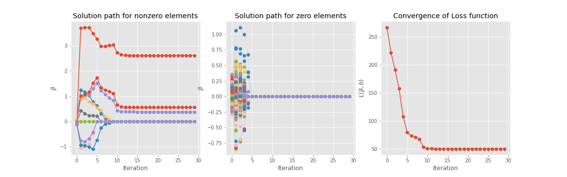
Remark 3: This approach can be viewed as an empirical Bayes approach as the hyper-parameter is learned from the data. Of most concern is that the empirical Bayes estimator has the risk of a degenerate solution (e.g., setting all ) in the high dimensional and very sparse setting, resulting in an inappropriate statement of the sparsity of the regression model (Scott and Berger,, 2010; Polson and Scott,, 2012; Datta et al.,, 2013). Next corollary demonstrates this issue.
Corollary 5.2.1.
Suppose and , using the empirical Bayesian estimator (14) for , then the model will fail to recover the signal if .
Proof. Suppose there exists estimator which can recover the signal, then . By Lemma 5.2, . Since , as . This implies that the model will shrink all the elements to zero, which contradicts the assumption that can recover the signal.
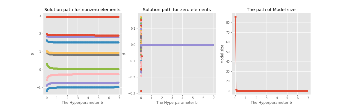
This phenomenon is empirically observed in Figure 1.This figure shows the solution path of in the same setting as Figure 2 in secetion 5.1. Here, seven of the ten nonzero elements have been estimated to be zero. One way to remedy this issue is to set (see Figure 2). In this case, the oracle properties of the and are guaranteed by Theorem 5.5.The exact value of hyper-parameter (determine the unknown constant) can be determined by the variable screening strategy as discuss in section 5.4. Here we provide the details of our CD optimisation algorithm in Algorithm 3:
where is some suitable small error tolerance, is the terminal number for the fixed point iteration, and is the value of the hyper-parameter chosen by the user.
5.2 Convergence analysis
In general, convergence of the loss function alone cannot guarantee the convergence of . Mazumder et al., (2011) showed the convergence of CD algorithms for a subclass of non-convex non-smooth penalties for which the first and second order derivatives are bounded. The authors also observed that for the type of log-penalty proposed by Friedman, (2012), the CD algorithm can produce multiple limit points without converging.
The derivative of the bridge penalty and its non-separable version are unbounded at zero, suggesting a local solution at zero to the optimization problem, this causes discontinuity in the induced threshed operators. Recently, Marjanovic and Solo, (2014) proved the convergence of the CD algorithm for the bridge penalty. Here, we show that the CD algorithm with the proposed non-separable bridge penalty also converges. We provide convergence analysis in the next two theorems. Details of the proofs can be found in section 7 of supplementary materials.
Theorem 5.3.
Suppose the data lies on compact set and the sequence is generated by where the map is given by equation (11) and , then
Theorem 5.4.
Let be the estimator obtained by the CD algorithm 3. Suppose satisfies A4 with , then is a strict local minimizer of . In other words, for any and
Proofs for the above theorems are given in Section 7 of supplementary materials.
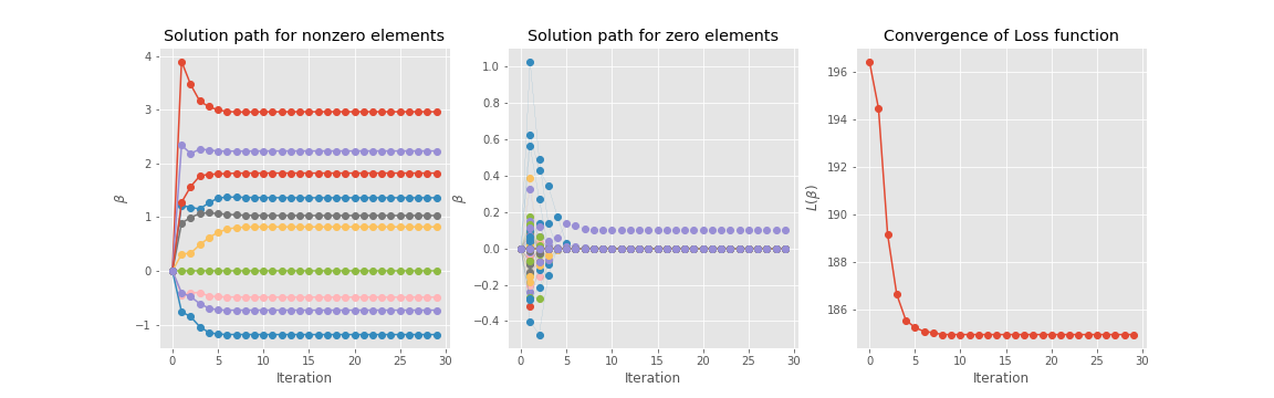
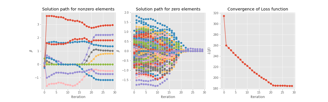
Empirically, we observe that convergence of the solution paths are pleasingly well behaved. Figure 2 demonstrates solution paths of the CD algorithm with different initialization strategies on a simulated sample of high dimensional regression problem with 990 zero entries and 10 nonzero entries in . The design matrix is generated with pairwise correlation between and equal to . Both the response and predictors have been standardized, so . Data is simulated with and . From figure 2, we see that two solution paths finally converge to the same local minima with only two mistakes (they failed to identify one nonzero element and to exclude one zero element).
5.3 Oracle properties
In this section, we study statistical properties of the non-separable bridge estimator. We will show that using , model consistency
and asymptotic normality of can be achieved.We state some additional assumptions here:
A6.
A7. There exist a constant such that as
A8. where
A9. where
Theorem 5.5.
Suppose assumption A1-A4, A6 to A7 are satisfied. Then under the following two cases,
(1): , or and assumption A8 holds.
(2): , and assumption A9 holds.
we have:
(a) Model consistency There is a strictly local minimizer such that
with probability tending to 1 and,
(b) Asymptotic normality With the local estimator , the correponding variance estimator from Equation (6) has the property that
Proof for the theorem can be found in section 8 of supplementary Materials.
5.4 Forward and backward variable screening
There are many variable selection techniques proposed in the literature, under a variety of assumptions, all of these estimator are shown to have variable selection consistency in high dimensional settings. Based on these result, it is not difficult to construct the variance estimator, which also has nice asymptotic properties. However, all the asymptotic arguments require some crucial assumptions about the sparsity of the underlying true model. For example, in this paper, it is assumed that the true number of nonzero is . In practice, we only have finite sample size and we are rarely certain about the sparsity level of the true model. It was found by Reid et al., (2016) that, the variance estimator from Fan et al., (2012); Sun and Zhang, (2012); Dicker, (2014) all suffer large biases in finite samples when the true underlying signals become less sparse (in Section 6.2, you will see that the posterior distribution of the variance is biased downwards). To overcome this bias, they suggest tuning the hyper-parameter in LASSO or SCAD by cross validation, which performs well over a broad range of sparsity and signal strength settings. Here, we propose a cross-validation free backward screening procedure for moderate to large sample problem and a forward screening procedure for small samples problem.
This is deployed as a path following warm up strategy. We begin with small(backward screening starting with big model) or big (forward screening starting with null model) value of hyper-parameter . The solution is used as warm-starts for next bigger or smaller value of and keep going with this fashion. When sample size is moderate to large, the solution path with respect to hyper-parameter from backward screening algorithm will stabilize automatically. Thus, in this case, it is cross-validation free. When the sample size is small, the solution path stabilizes slowly, it may ultimately threshold everything to zero. In this case, we run the forward screening with cross-validation to identify the hyper-parameter. Details of the procedures are included in section 4 of supplementary materials.
6 Simulation Study
In this section, we present some results from a set of simulations studies.
6.1 Comparison of PCG sampler effective sample size
In this section, we benchmark the PCG sampler scheme for prior with and against the Gibbs sampler scheme of (Park and Casella,, 2008) for the Bayesian LASSO and the Horseshoe prior (Makalic and Schmidt,, 2015) in the high dimension sparse regression setting. We included only these two schemes for comparison since in the high dimensional setting, very few MCMC schemes have closed form condition posterior, which are free of Metropolis -hastings proposal.
We simulate two sets of data with moderate correlation between the covariates, () and high () correlation for the design matrix with variables and sample size . The true vector is constructed by assigning 10 nonzero elements to location and setting all the remaining coefficients to zero. We set the variance of the error to 1 ().
For each data set, we ran 10 MCMC chains. Each chain generated 10,000 samples after an initial burn-in of 10,000. We calculated the effective sample sizes (ESS) based on the formula from Gelman et al., (2013). In Table 1, we report the maximum, minimum, median, average and standard deviation of ESS for across dimensions. Since all MCMC schemes considered here are based on normal mixture representations, they all need to generate from high dimensional gaussian distributions. All three schemes have the same computational complexity (Bhattacharya et al.,, 2016). Thus, if all their conditional posterior distribution have closed form expressions, there is not too much difference between their computational times. Thus, we only consider the indication about convergence rates, via their effective sample sizes here.
The effective sample size from the table shows that for the Bayesian LASSO, the PCG sampler () performs similarly to the traditional Gibbs sampler under all criterion, where the PCG sampler achieves a slightly higher ESS overall. The performances of both samplers do not appear to be sensitive to the increase in the correlation of the design matrix.
The PCG sampler for prior () significantly over performs the Horseshoe prior (using a Gibbs sampler) with respect to all the criterions. Here increasing the correlation of the design matrix has had a large effect on the ESS of both the Horseshoe Gibbs sampler and the PCG sampler. For the Horseshoe prior, the ESS has decreased by as much as 10 fold in some cases, and is particularly dramatic in the non-zero elements of . The PCG sampler is also impacted, with the worst case scenario being a seven fold decrease in ESS. However, comparing PCG to the Horseshoe prior, it can be seen that the PCG sampler is up to ten times more efficient in terms of ESS.
Finally, it should be pointed out that the proposed PCG sampler for the prior has one limitation in practice. Theoretically, it works for any , but in our python implementation, we found that when , numerical underflow is quite frequently encountered in the high dimension and very sparse setting. The problem worsens when , occurring even in very simple low dimension problems. When , the prior places increasingly more probability mass around zero. In this case, the full conditional posterior of , has a covariance matrix of the form , and is nearly singular. It seems that the 64-bit floating-point numbers in the numpy package from Python is not enough to keep the precision, therefore we restrict our numerical experiments to the case only.
| ESS | Max | Min | Median | Average | SD | Max | Min | Median | Average | SD |
| Bayesian LASSO Gibbs Sampler | Bayesian LASSO Gibbs Sampler | |||||||||
| 100053 | 24030 | 90496 | 86022 | 11814 | 100669 | 15986 | 92847 | 89595 | 10356 | |
| 86707 | 9806 | 38738 | 40636 | 21737 | 90138 | 10208 | 24451 | 36125 | 26440 | |
| All | 100053 | 9806 | 90317 | 85568 | 12779 | 100669 | 10208 | 92715 | 89060 | 11894 |
| PCG sampler | PCG sampler | |||||||||
| 100831 | 26760 | 91208 | 87218 | 10949 | 101525 | 21476 | 92851 | 89802 | 10604 | |
| 90860 | 10500 | 54789 | 47604 | 32152 | 91965 | 10399 | 31069 | 37976 | 26254 | |
| All | 100831 | 10500 | 91018 | 86821 | 12023 | 101525 | 10399 | 92805 | 89284 | 12022 |
| Horseshoe Gibbs Sampler | Horseshoe Gibbs Sampler | |||||||||
| 40536 | 1418 | 18854 | 18178 | 9194 | 53821 | 866 | 23564 | 23551 | 13492 | |
| 6772 | 943 | 3482 | 3554 | 1427 | 5729 | 90 | 2840 | 3151 | 1716 | |
| All | 40536 | 943 | 18530 | 18326 | 9266 | 53821 | 90 | 23331 | 23347 | 13578 |
| PCG sampler | PCG sampler | |||||||||
| 90564 | 12298 | 72514 | 67809 | 15355 | 92276 | 1614 | 69610 | 66323 | 16082 | |
| 37852 | 7166 | 20229 | 20355 | 10002 | 47088 | 1427 | 6768 | 13483 | 14627 | |
| All | 90564 | 7166 | 72093 | 67334 | 16022 | 92276 | 1427 | 69380 | 65794 | 16906 |
6.2 Performance of signal recovery in PCG and CD algorithms
In this section, we examine how prior recover signal under high-dimensional settings. We compare both the PCG algorithm and CD optimization algorithm with two well known Bayesian regression procedures, the Bayesian LASSO (Park and Casella,, 2008) and the Horseshoe (Carvalho et al.,, 2010). We also consider the penalized likelihood procedures: the MC+ penalty (Zhang et al.,, 2010) and non-separable spike-and-slab-lasso (NSSL) (Ročková and George,, 2018).
Similarly with the previous section, we construct the AR(1) correlation structure for design matrix with correlation . In Section 6.2.1, we test the performance of the model in both low and high dimensional settings under the following five setting when the number of nonzero regression coefficients is .
For each of the above scenarios, we repeated the experiment 100 times. Each time, the true vector is constructed by assigning 10 nonzero elements to random locations and setting all the remaining s to zero.Similarly, in Section 6.2.2, we consider the small sample size and all zero setting i.e., . In this case, for . We test two scenarios:
Finally, we also consider the very challenging case of small sample size and a less sparse problem (Reid et al.,, 2016) in Section 6.2.3 with , under the following two scenarios:
The true vector with 20 nonzero elements is constructed by duplicating the 10 nonzero elements and assigning them to random locations and setting all the remaining s to zero.
For all the Bayesian models, we assign a non-conjugate Jeffrey’s prior to . The Bayesian LASSO and prior use the hyper-parameter setting as discussed in Section 2.2. For the Horseshoe prior, we assign the hyper-prior to the hyper-parameter as suggested by Carvalho et al., (2010). We use posterior means of and as the estimator. Since the MCMC cannot provide a sparse solution directly, variables are selected by a hard thresholding approach where we perform the t-test based on the posterior samples, under the null hypothesis using as significant level.
For the optimization procedure, the hyper-parameter for the NSB penalty is chosen by using the forward/backward variable screening algorithm described in Section 5.4. The NSSL(Ročková and George,, 2018) is claimed to be cross-validation free. The popular MC+ penalty (Zhang et al.,, 2010) has two tuning parameter .
We applied the Sparsenet algorithm (Mazumder et al.,, 2011) to fit the MC+ penalty, which performs cross-validation over a two-dimensional grid of values . For NSSL, the variance is estimated by the iterative algorithm from (Moran et al.,, 2018). For NSB and MC+ penalties, we use the variance estimator from Equation (6).
In Tables 2 - 5, we report the simulation results by calculating the average of the following criteria from the 100 experiments: error(Root mean square error), error(Mean absolute error),FDR(False discover rate), FNDR(False non-discover rate),HD(Hamming distance),(variance estimator),(Estimated model size).We also report the standard derivations of the error, error, Hamming distance and the variance estimator among 100 experiments in the brackets. We use bold to highlight the best performance for each criteria among the full Bayesian procedure and optimization procedures respectively.
6.2.1 Sparse case with
| Full Bayesian procedure | Optimization procedure | |||||||
| Horseshoe | Bayesian | NSB | NSB | NSSL | MC+ | |||
| () | () | LASSO | () | () | ||||
| , , , | ||||||||
| L2 | 0.42(0.03) | 0.38(0.02) | 0.49(0.03) | 0.46(0.03) | 0.45(0.04) | 0.40(0.02) | 1.05(0.08) | 0.33(0.02) |
| L1 | 1.64(0.11) | 1.44(0.09) | 1.92(0.13) | 1.86(0.15) | 1.68(0.20) | 1.37(0.15) | 2.67(0.41) | 0.92(0.16) |
| FDR | 1.30 | 0.00 | 4.37 | 3.79 | 50.75 | 38.00 | 1.12 | 6.68 |
| FNDR | 0.06 | 6.65 | 0.00 | 0.00 | 0.00 | 0.00 | 11.13 | 0.00 |
| HD | 0.16(0.05) | 1.10(0.11) | 0.50(0.12) | 0.43(0.27) | 10.42(1.41) | 6.41(0.98) | 2.02(0.33) | 1.00(0.10) |
| 10.14 | 8.9 | 10.50 | 10.43 | 20.42 | 16.41 | 8.20 | 11.00 | |
| 3.01(0.35) | 3.13(0.14) | 2.96(0.24) | 3.01(0.40) | 2.96(0.31) | 2.97(0.20) | 1.69(0.40) | 2.99(0.21) | |
| , , , | ||||||||
| L2 | 0.41(0.04) | – | 0.25(0.04) | 1.15(0.19) | 0.15(0.02) | 0.13(0.01) | 0.14(0.02) | 0.21(0.02) |
| L1 | 9.15(1.77) | – | 2.90(0.88) | 26.82(2.98) | 0.37(0.06) | 0.35(0.04) | 0.37(0.08) | 0.61(0.16) |
| FDR | 4.68 | – | 2.16 | 47.67 | 0.73 | 0.00 | 0.00 | 10.00 |
| FNDR | 0.00 | – | 0.00 | 0.00 | 0.00 | 0.00 | 0.00 | 0.00 |
| HD | 0.51(0.10) | – | 0.20(0.06) | 10.4(1.21) | 0.03(0.01) | 0.00(0.00) | 0.00(0.00) | 3.06(0.54) |
| 10.51 | – | 10.20 | 20.40 | 10.03 | 10.00 | 10.00 | 13.06 | |
| 0.70(0.05) | – | 0.81(0.04) | 0.09(0.02) | 1.02(0.10) | 1.01(0.05) | 0.97(0.05) | 1.02(0.19) | |
| , , , | ||||||||
| L2 | 0.65(0.13) | – | 0.49(0.08) | 1.45(0.31) | 0.81(0.09) | 0.41(0.07) | 0.27(0.08) | 0.34(0.09) |
| L1 | 13.93(2.01) | – | 4.55(1.25) | 32.17(4.96) | 3.95(0.78) | 1.22(0.35) | 0.65(0.20) | 0.97(0.28) |
| FDR | 10.73 | – | 9.10 | 59.16 | 63.87 | 14.54 | 0.00 | 10.77 |
| FNDR | 0.00 | – | 0.01 | 0.00 | 0.00 | 0.00 | 0.00 | 0.00 |
| HD | 1.29(0.20) | – | 1.01(0.17) | 15.50(2.33) | 18.97(1.52) | 2.66(0.49) | 0.14(0.02) | 2.91(0.53) |
| 11.29 | – | 11.01 | 25.50 | 28.97 | 12.66 | 9.86 | 12.91 | |
| 2.06(0.18) | – | 2.43(0.16) | 1.20(0.15) | 2.39(0.13) | 2.88(0.10) | 2.95(0.01) | 2.97(0.14) | |
| Full Bayesian procedure | Optimization procedure | ||||||
| Horseshoe | Bayesian | NSB | NSB | NSSL | MC+ | ||
| ( | LASSO | () | () | ||||
| , , , | |||||||
| L2 | 1.19(0.21) | 0.80(0.15) | 3.86(0.66) | 0.81(0.17) | 0.70(0.15) | 0.71(0.19) | 0.64(0.19) |
| L1 | 14.05(2.57) | 9.40(2.05) | 40.27(5.35) | 2.06(0.73) | 1.65(0.37) | 1.62(0.40) | 1.80(0.41) |
| FDR | 1.11 | 1.02 | 59.00 | 0.21 | 0.21 | 0.20 | 16.62 |
| FNDR | 0.20 | 0.20 | 0.00 | 0.10 | 0.10 | 0.10 | 0.03 |
| HD | 2.10(0.22) | 1.80 (0.19) | 12.80(2.01) | 1.77(0.15) | 1.56(0.14) | 1.50(0.14) | 4.66(0.57) |
| 8.10 | 9.20 | 14.60 | 8.03 | 7.89 | 8.54 | 13.90 | |
| 0.02(0.01) | 0.10(0.02) | 0.25(0.05) | 1.30(0.10) | 1.44(0.11) | 1.10(0.11) | 1.10(0.14) | |
| , , , | |||||||
| L2 | 2.01(0.25) | 1.60(0.20) | 4.09(0.90) | 1.46(0.22) | 1.35(0.20) | 1.41(0.19) | 1.33(0.22) |
| L1 | 18.96(2.88) | 13.6(2.44) | 43.33(5.55) | 4.93(1.01) | 3.91(0.41) | 3.52(0.56) | 4.46(0.59) |
| FDR | 6.03 | 14.37 | 73.11 | 35.99 | 20.00 | 0.80 | 36.88 |
| FNDR | 0.36 | 0.20 | 0.44 | 0.19 | 0.20 | 0.30 | 0.16 |
| HD | 4.04(0.44) | 3.54(0.41) | 21.30(3.54) | 6.92(1.10) | 4.46(0.77) | 3.26(0.67) | 11.63(1.69) |
| 6.78 | 9.46 | 22.6 | 13.09 | 10.00 | 6.86 | 18.39 | |
| 0.44(0.1) | 0.77(0.21) | 0.20(0.05) | 2.49(0.30) | 3.02(0.20) | 3.68(0.41) | 2.91(0.22) | |
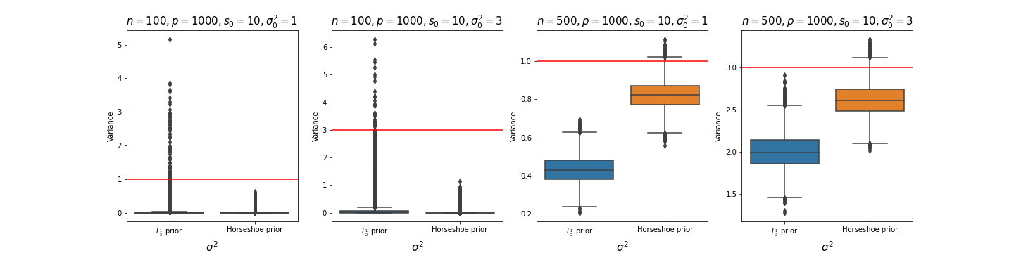
Tables 2 and 3 summarize the results of the simulation studies for . In low dimensional problems (), all approaches performed well. In high dimensional problems (), all except the Bayesian LASSO performed well. This is within our expectation as Castillo et al., (2015) showed that the Bayesian LASSO has poor posterior contraction rate in high dimensional problems.
One remarkable thing is the under-estimation of the variance by both and Horseshoe priors when . It was shown by Moran et al., (2018) that using the conjugate prior to can result in the under-estimation of variance in high dimension settings. However, as shown in Figure 3, when , using the non-conjugate prior for will also lead to under-estimation. This is because there exists spurious sample correlation with the realized noises in some predictors or between the predictor and response, even when they are actually independent (Fan and Lv,, 2008). As a result, the realized noises are explained by the model with extra irrelevant variables, leading to an underestimate of the variance (Fan et al.,, 2012).It can be seen that the marginal posterior distribution for has a heavy long tail and is biased downwards. Since the full conditional posterior of has a distribution, we conclude that most of the time, the MCMC sampler of overfits the model. Figure 3 also shows that when the sample size becomes large, this downwards bias becomes smaller.
Overall, among all the full Bayesian procedures, the prior with has the best performance in terms of error and error in the low dimensional case (Table 2). For the high dimensional case, the Horseshoe prior slightly out performs the prior with . The shrinkage of prior at is slightly weaker than the Horseshoe prior, consequently the variance estimates from Table 2 and 3 shows that while both procedures underestimate the variance parameter, the prior produces more severe under-estimation. Unfortunately, numerical underflow problem prevents us from using the prior with in high dimensional settings, we expect it could perform better than the Horseshoe and with priors, since the prior with has a strong shrinkage for values near zero. From Table 2, we see that this prior tends to select less and has a slightly higher value for the posterior mean of the variance parameter.
Amongst the optimisation procedures, in the low dimensional case, except for the NSSL penalty (which slightly under-performs), no procedure clearly dominated across all situations for all criteria. However, when we look at the high dimensional problem especially for the small sample size scenario (, Table 3), the performances of Bayesian and optimization procedures are comparable, except for the error where optimisation procedure out-performs the full Bayesian procedure.
All optimization procedure successfully targets the true variance and have lower and errors. It should be emphasised again that in the ultra high dimensional setting, the hyper-parameter in NSB penalty is determined by a cross-validation based strategy and we believe this is the key to success. The hyper-parameter in MC+ penalty is always determined by cross-validation in all scenarios.
6.2.2 No signal case
Table 4 shows the performance of the models under the setting with small sample size , and no signal (). It is apparently that, the full Bayesian procedure out-performs the optimization procedure under criteria which measure the performance of variable selection (i.e. FDR,FNDR,HD and ). Both the NSB penalty and MC+ penalties provide reliable variance estimation, but this is not the case for NSSL penalty. The NSSL selects too many variables and thus underestimates the variance.
Table 4 provides further evidence that, compared with the Horseshoe, the prior with provides relatively weaker shrinkage at values near zero. We can also see that the with again produces smaller variance estimates, although the underestimations are not severe in this setting. In addition, the NSB penalty with tends to select more variables than NSB penalty with .
| Full Bayesian procedure | Optimization procedure | ||||||
| Horseshoe | Bayesian | NSB | NSB | NSSL | MC+ | ||
| ( | LASSO | () | () | ||||
| , , , | |||||||
| L2 | 0.09(0.01) | 0.08(0.01) | 0.10(0.01) | 0.09(0.01) | 0.07(0.01) | 0.72(0.11) | 0.14(0.02) |
| L1 | 1.96(0.15) | 0.92(0.10) | 1.41(0.24) | 0.21(0.03) | 0.12(0.02) | 2.78(0.32) | 0.37(0.04) |
| FDR | 0.00 | 0.00 | 0.00 | 42.00 | 40.00 | 100.00 | 99.00 |
| FNDR | 0.00 | 0.00 | 0.00 | 0.00 | 0.00 | 0.00 | 0.00 |
| HD | 0.00(0.00) | 0.00(0.00) | 0.00(0.00) | 3.18(0.18) | 1.42(0.10) | 13.41(1.17) | 5.82(0.50) |
| 0.00 | 0.00 | 0.00 | 3.18 | 1.42 | 13.41 | 5.82 | |
| 0.75(0.07) | 0.85(0.07) | 0.75(0.07) | 0.92(0.03) | 0.95(0.02) | 0.60(0.03) | 0.90(0.03) | |
| , , , | |||||||
| L2 | 0.10(0.01) | 0.13(0.02) | 0.07(0.01) | 0.13(0.01) | 0.17(0.02) | 0.95(0.15) | 0.20(0.03) |
| L1 | 1.11(0.12) | 1.21(0.11) | 1.94(0.28) | 0.38(0.04) | 0.38(0.04) | 3.73(0.30) | 0.66(0.05) |
| FDR | 0.00 | 0.00 | 0.00 | 33.33 | 41.00 | 100.00 | 98.00 |
| FNDR | 0.00 | 0.00 | 0.00 | 0.00 | 0.00 | 0.00 | 0.00 |
| HD | 0.00(0.00) | 0.00(0.00) | 0.00(0.00) | 3.22(0.20) | 2.58(0.23) | 7.89(0.40) | 7.60(0.44) |
| 0.00 | 0.00 | 0.00 | 3.22 | 2.58 | 7.89 | 7.60 | |
| 2.50(0.08) | 2.74(0.10) | 2.45(0.23) | 2.80(0.07) | 2.75(0.06) | 1.20(0.15) | 2.64(0.10) | |
6.2.3 Less sparse case
Here we consider the less sparse case with and we set , (small sample and high dimensions). We see that whereas all the algorithms in the high dimensional, small sample, but very sparse setting (, Table 3) behave reasonably well and similarly to each other, their performances deteriorate when the sample size is small and true underlying model become less sparse(, , ), see Table 5.
Comparing the result from Table 3 and 5, the full Bayesian procedure shows deterioration of the estimation error (i.e. , and ). The higher Hamming distance(HD) from all the models indicates that neither the t-statistic test from MCMC nor the thresholding operator from optimization provides reliable variable selection. In this difficult situation, the NSB penalty with shows superior performance in terms of estimation. Our result is consistent with Reid et al., (2016), who also investigated the similar less sparse scenario. They recommended using the cross-validation strategy. We followed their recommendation and proposed forward variable screening with cross-validation strategy to determining hyper-parameter .
| Full Bayesian procedure | Optimization procedure | ||||||
| Horseshoe | Bayesian | NSB | NSB | NSSL | MC+ | ||
| ( | LASSO | () | () | ||||
| , , , | |||||||
| L2 | 4.03(0.50) | 2.06(0.33) | 6.17(1.03) | 1.74(0.30) | 1.33(0.27) | 2.96(0.33) | 1.32(0.25) |
| L1 | 39.01(4.05) | 20.14(3.24) | 68.54(6.71) | 8.26(1.60) | 5.70(0.81) | 10.83(1.70) | 6.31(0.99) |
| FDR | 0.00 | 0.00 | 0.00 | 47.65 | 27.00 | 0.64 | 53.00 |
| FNDR | 1.70 | 0.70 | 1.96 | 0.26 | 0.19 | 1.00 | 0.10 |
| HD | 16.11(2.01) | 6.96(1.05) | 19.60(2.55) | 18.56(1.88) | 8.98 (0.88) | 9.86(0.90) | 28.79(2.03) |
| 3.89 | 13.04 | 0.40 | 33.40 | 25.00 | 10.24 | 46.25 | |
| 0.20(0.01) | 0.31(0.01) | 0.55(0.03) | 1.35(0.10) | 1.29(0.10) | 2.41(0.22) | 1.40(0.13) | |
| , , , | |||||||
| L2 | 4.64(0.60) | 2.93(0.40) | 6.17(1.35) | 3.20(0.60) | 2.79(0.31) | 4.16(0.44) | 3.23(0.30) |
| L1 | 49.41(5.05) | 24.58(4.00) | 70.1(6.80) | 16.05(2.31) | 12.67(2.01) | 16.06(2.03) | 15.98(2.44) |
| FDR | 0.00 | 0.83 | 0.00 | 59.06 | 43.00 | 0.00 | 56.00 |
| FNDR | 1.75 | 1.11 | 1.97 | 0.66 | 0.60 | 1.32 | 0.66 |
| HD | 17.46(2.31) | 11.15(1.55) | 19.7(2.60) | 24.46(2.32) | 16.92(1.88) | 13.33(1.67) | 34.54(3.48) |
| 2.54 | 8.84 | 0.30 | 33.46 | 24.62 | 6.99 | 41.94 | |
| 0.25(0.03) | 0.43(0.04) | 0.89(0.20) | 3.32(0.33) | 3.66(0.30) | 3.69(0.35) | 1.05(0.08) | |
7 Conclusion and Discussion
In this article, we proposed an exact scale mixture of normal representation of the exponential power prior with . Based on this representation, we developed an efficient MCMC sampling scheme with faster convergence rate than traditional Gibbs sampling scheme and it is scalable to high dimensional problem. The normal mixture representation allows the sparse prior to be easily extended to the generalized linear model and other regression setting with only slight modifications to the MCMC scheme.
In addition, inspired by the full Bayesian approach of the exponential power prior, we formulated a non-separable bridge penalty. This is done by integrating out the hyper-parameter in the bridge penalty with respect to some suitable choice of hyper-prior. The NSB penalty yields a combination of global-local adaptive shrinkage and threshold. With the gaussian likelihood, its KKT condition lends itself to a fast optimization algorithm via coordinate-descent. Since the NSB penalty is a non-convex, non-separable and non-lipschitz function, we also provide a theoretical analysis to guarantee the convergence of the CD algorithm. Both the PCG sampler and CD optimization algorithms are not limited to the gaussian likelihood, examples of extensions of our algorithm to more general settings can be found in Section 5 of Supplementary Materials.
One limitation of our MCMC scheme is the numerical underflow in high dimensional problem when . For sufficient large, we are close to the penalty. We anticipate that such prior may attain sharper than current nearly optimal contraction rate. It may also lead to better empirical performance in high dimensional settings than the existing global-local shrinkage priors. In fact, we have already observed the superior performance when in low dimensional problems. We hope that, in the future, we can overcome the numerical underflow issue at least for the case. Another future research area is the uncertainty quantification of the optimization results. One potential direction is to look at ensemble learning with Bayesian bootstrap, which is processed by sampling multiple weight vectors using a Dirichlet distribution and fitting multiple penalized weight least square models. One could study whether the induced randomness provides good uncertainty quantification.
Supplementary Materials
Section 1. Normal-mixture representation of exponential power prior
Section 2. Derivations of Partially Collapsed Gibbs Sampler
Section 3. The KKT condition of non-separable bridge penalty
Section 4. Forward and backward variable screening
Section 5. Extension to logistic model
Section 6. Posterior consistency and contraction rate
Section 7. Convergence analysis of the coordinate descent algorithm
Section 8. Oracle property
1. Normal-mixture representation of exponential power prior
Proof of Lemma 2.1
Proof.
If is a Laplace transformation of some non-negative function evaluated at , then is the inverse Laplace transformation
where .
Let , then . Following this rearrangement, we can put a laplace prior on conditionally on ,
We can construct a laplace-gamma mixture representation for exponential power prior with
To get another parametric form, move the hyper-parameter outside the gamma distribution, and apply the change of variable in the right hand side of the above equation. Let , then we have
where and . ∎
Proof of Lemma 2.2
Proof.
Write
then is the Laplace transform of of some non-negative function evaluated at , where .
Let , then . Following this rearrangement, we can put a exponential power prior with on conditional on then,
We can see that the exponential power prior with is the mixture of exponential power prior with and
Using a similar argument as in the proof of Lemma 2.1 moving the hyper-parameter outside the gamma distribution by using the change of variable trick. We let , then
∎
Proof of Theorem 2.3
Proof.
Starting with the decomposition given in Lemma 2.2, we make some further decompositions. Our argument consists of three steps:
Step 1: Set , then
Step 2: Apply Lemma 2.2 again with , then
Step 3: By change of variables, set , then
Using the above three step argument recursively, then for any , we have
Consequently, the exponential power prior with can be written as
for . Since it is well know that the laplace distribution can be represented as a normal exponential mixture. ∎
Some intuitions for the prior
We now provide some intuition as to why the prior is suitable as a sparsity prior. We carry out the illustrations in terms of the simpler normal mean model. Our treatment is the same as Carvalho et al., (2010). Suppose that we observe data from the probability model for . Here the primary goal is to estimate the vector of normal means and a secondary goal is to simultaneously test if the ’s are zero. To do that, we consider the Bayesian method by applying the sparsity inducing prior to . We focus on the posterior mean, which is known to be optimal under quadratic loss. The global-local shrinkage prior can be represented as and
For simplicity, we further assume . Then the Bayes estimator for under quadratic loss is
hence by Fubini’s theorem, the marginal posterior mean is
Reparametrising with , then can be viewed as a shrinkage factor, where means no shrinkage and means total shrinkage to zero.
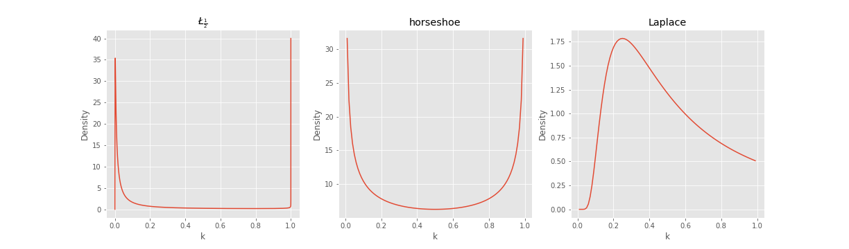
For the exponential power prior with , the inducing density of is given by
Figure 4 demonstrates the behaviour of the prior with (left panel), as well as the Horseshoe prior (middle panel) and the Laplace (Bayesian LASSO) prior (right panel).
The prior shares much similarity to the Horseshoe prior, both mimic the behavior of the spike-and-slab prior, putting large probability mass around and . The prior starts from zero, then dramatically increase to a first peak at near zero and finally follows a U-shape that is very similar to the Horseshoe prior. In addition, its density function is almost zero for .
For the more general case, there is no analytic expression for the density of , and it is difficult to numerically illustrate the density. Intuitively as becomes larger, tends to zero, the density of will degenerate to two points and , because the prior converges to an improper spike-and-slab prior , induced by the norm, and denotes the dirac mass function. In other words, as tends to zero the density of will degenerate to two point mass with and . Under the sparse normal mean model, we have
and the corresponding posterior mean for is given by
with .
2. Partially collapsed Gibbs sampling
Steps for PCG sampler
Here we give the details of the three steps that comprise the PCG sampler, for sampling the parameters under the prior with .
Step M: Marginalise
Step P: Permute
Step T: Trim
We use superscript to present intermediate quantities that are sampled but not retained as part of the output. Step M is generalisation of the traditional Gibbs sampler with some components being updated multiple times within each iteration.
In the second step we rearranged the ordering of the update in Step M by swapping the ordering of steps 5 and 6 with steps 2,3 and 4. This step does not alter the stationary distribution of the Gibbs sampler. Finally, the intermediate draws of and are not necessary if we can sample and in steps 2 and 3 directly from the respective marginal distributions, so trimming the intermediate Steps 2 and 3, we arrive at the last set of updating procedure.
Derivations of conditional posteriors
Since
with . The conditional posterior is a gamma distribution with shape parameters and .
Next, we derive the conditional posterior for . Observe that given , is conditionally independent of the remaining s. In addition, given , is also conditionally independent of and b. Thus,
From Theorem 2.3, we see that
Thus,
since sampling the generalized inverse gaussian distribution is not easy, we can sample from the inverse gaussian distribution.
3. The KKT condition
Proof of Theorem 5.1
Proof.
When , taking yields
| (15) |
and . Thus, without loss of generality, we assume .
Step 1: We first show that there exists a hard threshold in the KKT condition. When is the solution, define
Then
| (16) | ||||
therefore, is minimised at where . i.e., satisfy the following equation
| (17) |
with minimum value
Re-writing Equation (15) as
we see that has no solution when , in this case, .
For , there exists at least one solution. As is strictly increasing when , there exists such that .
Step 2: Next, we show the convergence of fixed point iteration at .
Let
we need to check that
is follows from the definition of . We see that for
Using the fact that , we have
Thus, . Now we show that is a a contraction mapping on . We have and . Since , for . Therefore, is a a contraction mapping on . Since is complete, by Banach fixed point theorem, there exists one and only one fixed point such that
| (18) |
Step 3: Up to now, we showed that when , there exists a such that the KKT condition is satisfied. We haven’t precluded the potential solutions , which also satisfies the KKT condition. Now we want to claim that is the only local minimum for given the parameters in other dimension are fixed. We write the descent function
| (19) | ||||
where . Then it is easy to see that
where the derivative is taken with respect to . Since and , we see that for and for . Thus, if there exists such that , then can only be the local maximum. is the only local minimum.
Step 4. To find the global minimum when , we need to check the value of descent function because we couldn’t preclude the case that is the global minimum. To see the existence of this potential case, we provide a constructive proof.
Suppose , plug in (18) into (19), then we have
we have if
Thus, there exists sufficient small such that for , the inequality above will hold. We rewrite Equation (18) as
Since for , by implicit function theorem, there exists such that . In addition, the fixed point iteration guarantees that is a one to one map for . By Equation (18), it is easy to see that is a monotonic increasing function. Hence, for the inequality will hold. By Lemma 5.2 in the main paper, we have and
where . By setting sufficient small, it is possible to construct such that
∎
Proof of Lemma 5.2
Proof.
From Equation (10) in the main paper, we plug into , then
By arranging , we have
for . Therefore,
Since we have , it follows directly that
∎
4. Forward and backward variable screening
In this section, we provide details of the proposed backward and forward variable screening algorithms. The backward screening algorithm does not use cross-validation, and is recommended for when the sample size is moderate to large. For small sample size, a forward variable screening algorithm cross-validation is recommended.
Consider a sequence of parameters with , the CD optimization begins with hyper-parameter . In default, we set . The first output is then used as a warm start for the 2nd iteration of the CD optimisation with . The algorithm continues in this fashion and we can visualise the entire solution path of with respect to the hyper-parameter . Since the function is continuous, this assures that a small perturbation in will lead to only small changes in the solution for , this suggests that using the solution of the previous optimisation for the next one is a reasonable strategy. The backward screening algorithm is provided in Algorithm 4.
Roughly speaking, the higher the value of , the more the estimated are set to zero. Hence we use the term backward variable screening. The algorithm starts with a big model and gradually removes insignificant coefficients. When the sample size is relative large, the solution path stabilizes very quickly with increasing values of (See Figure 5). In fact, we found that, when the sample size is large, we can fit the model directly by setting , but we still recommend backward variable screening because we don’t know how large the sample size needs to be.
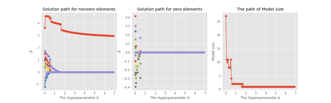
When the sample size is small, the solution path stabilizes slowly, it may ultimately threshold everything to zero, requiring cross-validation to identify the best solution. Figure 6 shows the solutions paths from a simulated example with and . We can see that the model quickly shrinks all coefficients to zero. In such cases, we found that a forward screening strategy, together with cross-validation, works better. Although cross-validation is computationally intensive, it was found by Reid et al., (2016) that it guarantees a robust performance for small sample size and less sparse models. Our numerical experiments are consistent with the numerical results in their paper.
Here we develop a forward variable screening algorithm with K-fold cross-validation. We first reparametrize the hyper-parameter to . Then we consider a sequence of increasing parameters with and . In default, 100 evenly spaced points have been used. We use the same re-initialization strategy as backward variable screening. The optimization output from the previous value of is used as a warm start for optimization at current . For each , we obtain solutions of from the -fold cross-validation. Once we have the optimal value of , we fit the model to the entire data set with forward strategies. Empirically, we found the forward strategies did better than backward strategy when the sample size is small and the model is less sparse.
The sure independence screening by Fan and Lv, (2008) can be viewed as a backward strategies. They greatly simplified the original ultra-high dimensional problem into a low-dimensional one and then fitted the model with LASSO or SCAD penalty. In another direction, Wang, (2009) investigated the forward regression in ultra-high dimensional problems. Our forward variable screening strategies can be viewed as a smooth version of forward regression. Wang, (2009) used the BIC criterion to select the optimal model size. They show screening consistency for their approach. Here, we determine the optimal model by cross-validation. For infinite sample size, the performance of our forward and backward screening algorithms are guaranteed by the oracle properties of the non-separable bridge penalty. We provide the description of forward screening algorithm in Algorithm 5.
5. Extension to logistic model
PCG sampler for Bayesian logistic model
The global-local scale mixture of gaussian representation for the prior allows us to extend the PCG sampler to the model which can be expressed as gaussian mixtures or the likelihood which are conjugate with gaussian priors. For example Bayesian quantile regression under asymmetric Laplace distributions (Yu and Moyeed,, 2001) and logistic regressions.
Here we only show how to extend the result to the logistic regression models with binomial likelihood and a logistic link function. We do that by using the data-augmentation trick in logistic model proposed by Polson et al., (2013). Applying their technique here, let be the number of successes, the number of trials and the vector of predictors for observation . Let , where is the log odds of success. The likelihood for observation is
where and is the density of a Polya–Gamma random variable with parameters . Then, conditional on , we have a gaussian likelihood of the form
where and . let the prior be assigned to , then we can construct the PCG Sampler scheme:
where . Here we have just slightly modified the conditional posterior for and replaced the conditional posterior of with . The construction of the PCG sampler is similar to Section 2.
Coordinate descent with Proximal Newton map
In this section, we extend the coordinate descent algorithm from gaussian likelihood to the binary logistic likelihood. Our strategy is the same as Friedman et al., (2010). By coding the response as , the likelihood can be written as
If we apply the Newton algorithm to fit the (unpenalized) log-likelihood above, that is equivalent to using the iteratively reweighted least squares algorithm. For each iteration, we solve
| (20) |
where and is diagonal matrix of weights.
For logistic regression with non-separable bridge penalty, the fitting algorithm consist of two steps. First, we create an outer loop, which computes the quadratic approximation of (unpenalized) log-likelihood as in (20) based on the old from last iteration. Then in the inner loop, we use coordinate descent to solve the penalized weighted least-squares problem
| (21) |
The solution to equation (21) in the inner loop is known as Proximal Newton Map (Lee et al.,, 2014). By slightly modifying the coordinate descent algorithm for penalized least square problem in Section 5.2, we can get the coordinate descent algorithm for penalized weighted least square problem.
6. Posterior consistency and contraction rate
Assuming that the observations consisting of independent observations with product measure , where . If the measure with density is considered random and distributed according to , as it is the case in Bayesian inference, then the posterior distribution is the conditional distribution of based on the prior
where and is a -field on .
The posterior is said to be weakly consistent if it concentrates on arbitrarily small neighborhoods of the true , , in -probability tending to 1 as or strongly consistent if this convergence is in the almost-sure sense. We study the rate at which the neighborhoods of may decrease to a small ball while still capturing most of the posterior mass, in the weak sense (See Chapter 6 of Ghosal and Van der Vaart, (2017)). Note that in high dimensional regression setting our prior depends on the number of predictors, and hence sample size dependent, therefore we use to denote this dependence.
The following notation will be used in this section and in proving the oracle property in a later section: we rewrite the dimension of the model by to indicate that the number of predictors can increase with the sample size . We use and to indicate true regression coefficients and the true standard deviation and . Let be the set containing the indices of the true nonzero coefficients, where , then denotes the size of the true model. The -covering number of the space with respect to a metric is denoted by , which is the minimal number of -balls of radius needed to cover . We further let denote the design matrix corresponding to the model , and use to abbreviate , finally we use and to denote inequality up to a constant.
We make the following assumptions on contraction theorems:
- A1.
-
The dimensional is high, with and .
- A2.
-
The true number of nonzero is , where .
- A3.
-
All the covariates are uniformly bounded. In other words, there exists a constant such that for some .
- A4.
-
There exist constants , and an integer satisfying and , so that for any model of size .
- A5.
-
and E is some positive number independent of .
Some preliminary results
Before proving the posterior contraction rates, we first state and prove some auxiliary results.
Lemma 7.1.
Suppose that assumptions A1, A2 and A5 hold, the exponential power prior with and , satisfies
| (22) |
| (23) |
where are positive constants and .
Proof.
It is easy to see that
with the second equality holds.
To prove the Equation (22), first we show that for any , the following equation,
| (24) |
hold. We then prove Equation (22) holds for the special case . Then the more general case will trivially hold by using Equation (24).
To prove Equation (24), it is enough to show
where . Consequently, it is sufficient to show
for any . Since , then for sufficient large we just need,
We see that the above inequality hold since as
Since the exponential power prior with has the Laplace-Gamma mixture representation with and , we write
where is the density of . In the fifth line, the equality is obtained by applying the mean value theorem to the first term with . In the last line, the inequality is obtained by applying the Chernoff bound to the tail of Gamma distribution. The Chernoff bound for Gamma distribution is if , otherwise it is 1. Hence, the value of we choose should satisfy the constraint .
Now, we set , then we have
for some and .
∎
Lemma 7.1 shows that the exponential power prior with can balance the requirement of putting enough mass around zero and tail thickness. It is easy to verify that the Bayesian LASSO fails to satisfy the properties in Lemma 7.1 unless assumption A5 changes to and we set (Song and Liang,, 2017). This assumption is unrealistic as it requires the magnitude of to asymptotically decrease to zero. Next, we provide an upper bound for the covering number in Euclidean space.
Lemma 7.2.
For , and , for any , we have
The proof for Lemma 7.2 can be found in Appendix C of Ghosal and Van der Vaart, (2017).
Now, we derive the analytical expressions based on the Renyi distance for two Gaussian distributions.
Lemma 7.3.
Consider the root of average Renyi divergence of order ,
where and are their density function. Let and be the law of the random variable with Multivariate Gaussian distribution and respectively. Then
Proof.
To simplify notation and apply change of the variable in the later part of the proof, we set .
Thus,
We can see that both the first and second term are non-negative and if and only if and . The symmetric property is also easy to see. ∎
Finally, we restate a simple version of Lemma 8.21 from Ghosal and Van der Vaart, (2017), which will help us to prove Theorem 6.2.
Lemma 7.4.
For any and ,
Proof of the contraction theorem
The key to our proof will be drawing upon the framework of posterior concentration theory for independent but not identical observations from the Theorem 1 of the seminal paper by Ghosal et al., (2007). Theorem 1 provides a very general framework for showing posterior concentration in infinite-dimensional models. The contraction rate is described in terms of the average squared Hellinger distance by default. However, as mentioned by Ning et al., (2020), closeness in terms of the average squared Hellinger distance does not imply that the posterior means of the parameters in the two densities are also close on average in terms of the Euclidean distance. To alleviate the problem, we use the root of average Renyi divergence of order as distance. We will construct a likelihood ratio test and then show that such a test works well for this distance. Finally, we show that the posterior consistency under this new distance implies the the posterior consistency under the Euclidean distance.
Restating Theorem 1 of Ghosal et al., (2007) here, suppose that for a sequence with and , there exists constants , and a sequence of sieves , where is the sample space (model space) of the prior distribution, such that if the following three conditions hold:
1. Prior concentration condition:
| (25) |
where and
2. Sieve sequence condition:
| (26) |
for some and
3. Testing conditions:
There exists a sequence of test function such that
| (27) | ||||
Then for sufficiently large M, in probability.
Before begin the proof, we defined the sieve by using the concept of generalized dimension (Bhattacharya et al.,, 2015; Song and Liang,, 2017; Ročková and George,, 2018), which approximates the model size. We define the generalized dimension as
where and . Then we can define the sieve as
Proof of theorem 3.1
Proof.
Part 1. Prior concentration condition:
Let and . Then we have:
Thus,
Since
we set ,, , ,
with
By arranging the terms, we have:
Since ,
For , considering the Taylor series centered at 1, we have
We see that
Define the two events and as follows:
Condition on , we see that
The last inequality is by assumption A1. Then we have:
First, we give a lower bound to . Since , we have
Next, we derive the lower bound for . Condition on and by assumption A3, we have
Define , we have . Thus,
for some . The fourth and fifth inequality are from Lemma 7.1. The final inequality is by using the fact that the second term dominates the first term and the third term is asymptotically 1.
Combining all the result above, we have
where .
Part 2. Sieve sequence condition:
First,we show the existence of sieve set such that
we choose with constant and define as:
It is easy to see that:
We now show . For term , we see that
where . By Lemma A.3 in Song and Liang, (2017), we have
where
.
Therefore, to show , it sufficient to show that
For the first term of , by Lemma 7.1, , we have:
The last inequality will hold for sufficient large because the term always dominates . We set , then we have
For the second term of , we have
Consequently,
For term , when is large, it is sufficient to show that
Since is Gamma distributed with shape parameter and scale parameter ,applying the Chernoff bound to Gamma distribution and choosing as any positive constant such that , we have
Therefore,
where the second is obtained by the upper bound for .
For term
where the first inequality is followed by using the Chernoff bound to Gamma distribution with shape parameter and rate parameter and the second inequality is followed by assumption A2.
For term :
Part 3. Testing conditions:
When the variance is unknown, techniques from Ghosal et al., (2007); Ghosal and Van der Vaart, (2017) can not be applied directly. Instead, we follow Ning et al., (2020)’s approach by constructing the likelihood ratio test with the sieve broken up into small pieces. More precisely, we perform tests in small covering pieces such that
| (28) |
where and are parameters which belong to the probability density and respectively.
In each piece, we consider testing against with
and . To do that, we use the likelihood ratio test
which is the most powerful Neyman-Pearson test.
Since ,
then by Markov inequality
For the type II error, by Cauchy-Schwartz inequality
Thus, if we can show that
for very small c, then our work finish.
To see this, observe that
| (29) | ||||
Because and ,we obtained the upper bounded
where the third inequality is by assumption A3, the fourth inequality is obtained when and are sufficient close( sufficient large). To complete the construction of the test, we need to show that , where is the number of covering pieces for sieve satisfying . We see that
where in the first term of the second inequality, we are using the fact that with . We already show that in probability. Now we want to argue this implies the posterior consistency in terms of Euclidean distance.
By lemma 3, we see that implies
The first inequality above implies that
For sufficient large, there exists such that , we have . This implies that . By assumption A4 and Theorem 3.2 for sufficient large, the second inequality implies Consequently, we have
in probability. ∎
Proof of theorem 3.2
Proof.
We define the set of event for some positive constant and . Then
We have that:
For the first term of right hand side, we have:
In part 2 of the proof of Theorem 3.1, we see that
For the second term of the right hand side, by applying Lemma 7.4, we have
Combining the two results, we have:
consequently, as , . ∎
7. Convergence analysis
Theorem 5.3 will follow directly by the Lemmas below.
Lemma 7.5.
The sequence , returned by the CD algorithm is a bounded sequence.
Proof.
Given the initial sequence , then the entire sequence belongs to the sub-level set . This is easy to see as the convergence of loss function is guaranteed by Theorem 5.1, which shows that we can achieve the steepest descent in each coordinate. Since for any , , this implies that is bounded for any . This completes the proof. ∎
Lemma 7.6.
Define the descent function as:
where is the loss function for with all other parameters held fixed. Then if and only if .
Proof.
We show that if , then . For the reverse direction, the result is trivial.
Case 1. . In this case, is the unique univariate global minimizer of . Thus, implies .(The uniqueness of global minimum is shown in the step 3 and step 4 of the proof of theorem 5.1).
Case 2. . In this case, the unique univariate global minimum attains at both and . By the rule of map (see Theorem 5.3), we have
. If , then . If , implies .
Case 3.. In this case, is the unique univariate global minimizer of . Thus, implies .
Case 4 . In this case, is the unique univariate global minimizer of . Thus, implies .
∎
Lemma 7.7.
Suppose there exists two convergent subsequences and
such that and . Then their differences converge to zero:
Proof.
First, we want to check the continuity of some functions. We write and .
Then the continuity of is clear.
We see that both
and are continuous maps.
From step 1 of the proof of theorem 5.1, is the unique solution of the equation
Since , then by implicit function theorem, is continuous. Therefore, the the composition function is continuous. Consequently, if , we also have and .
Next, we want to show that . We focus on the th coordinates for arbitrary . Without loss of generality, we assume . The result from the negative side can be obtained by symmetry. We consider the problem in three cases:
Case 1. . By convergence of the subsequence , there exists sufficient large such that for any , we have . In this case, . We have .
Case 2. . By convergence of the subsequence , there exists sufficiently large such that for any , we have . By step 2 and step 3 of the proof of theorem 5.1, there exists local minimizer and is the unique solution of the equation
From the step 1 of the proof of theorem 5.1, we also see that for any , by implicit function theorem, there exists continuous and differential function for . In addition, is one-to-one map. Hence, if we have and , this implies . By continuity of , we also have
Now, we can further consider three sub cases:
a. . There exists a sufficiently large such that for any , we have . Then . Taking the limit on both sides, .
b. . There exists a sufficiently large such that for any , we have
. Then . We have .
c. . There exists a sufficiently large such that for any , will approach zero from only one side. Suppose this is not true, then . In other words, will converge to a limit set rather than a limit point which contradicts the assumption in the lemma.
If approach zero from the right side. Then,
Therefore we have, , which also implies .
If approach zero from the left side. Then, and . This implies that and . By the rule of ,
Taking the limit of , we have .Therefore . Finally, we use Lemma 6 to finish the proof. By continuity of descent function, we have
since Theorem 5.1 guarantees the non-increasing of the loss function, is decreasing and bounded below by zero. Therefore,
We have already shown that , then by Lemma 6, if and only if . ∎
Proof of Theorem 5.4
Proof.
We decompose the perturbation into two disjoint set: where and . Then, we have
where the last inequality is followed by assumption A4. By mean value theorem, there exists such that
Plug in and , we have
where the last inequality holds for sufficiently small. Combining all the upper bounds we obtained above, we have
where
Now we treat each term separately,
where , and the second inequality follows by Theorem 5.1. the KKT condition. Again, by KKT condition in Theorem 5.1, we have
∎
8. Oracle properties
Proof of Theorem 5.5
We only show the case (2): , and assumption A9 holds. The argument for case (1) is exactly the same, so we will omit the details.
Proof.
Let be the oracle estimator. We want to show that, with probability tending to 1, the oracle estimator is a strictly local minimizer of . By theorem 5.1, it suffices to show that, with probability tending to 1, satisfies the KKT conditions:
plug in into the KKT condition, we see that
| (30) |
by mean value theorem, we have
| (31) | ||||
from some such that . Consider the events
By standard Gaussian tail bounds (Wainwright,, 2019), we have
By assumption A4, is invertible, then under event , we have
where the last inequality is followed by assumption A2. In addition, for sufficient large, under event and assumption A5, we have , which implies that . By Lemma 5.2, we have
where by Equation 31 and assumption A6. Define the event
then by assumption A7, . Therefore, it suffices to show that for sufficiently large under the event the KKT condition will statisfy. For and sufficient large, under event , we have
For and sufficient large, under event , we have
where the last inequality is followed by assumption A8. Next, we want to check that, for and sufficient large, under event , we have
| (32) |
where . Since , it suffices to show
We see that under event , , thus it suffices to show
where . By assumption A6, and , we have:
where is some positive constant. Finally, we want to check that, for and sufficient large, under event , we have .
| (33) |
Since for , plug in (8.3) into (8.4), then we have
We see that to show , for sufficient large and under event , that is equivalent to show
By assumptions A5,A6 and , taking , for the left hand side, we have
while for the right hand side, . The result follows immediately. Now we show the asymptotic normality of . Under the event , as
Hence, we have
∎
References
- Andrews and Mallows, (1974) Andrews, D. F. and Mallows, C. L. (1974). Scale mixtures of normal distributions. Journal of the Royal Statistical Society: Series B (Methodological), 36(1):99–102.
- Armagan, (2009) Armagan, A. (2009). Variational bridge regression. In Artificial Intelligence and Statistics, pages 17–24.
- Bhattacharya et al., (2016) Bhattacharya, A., Chakraborty, A., and Mallick, B. K. (2016). Fast sampling with gaussian scale mixture priors in high-dimensional regression. Biometrika, page asw042.
- Bhattacharya et al., (2015) Bhattacharya, A., Pati, D., Pillai, N. S., and Dunson, D. B. (2015). Dirichlet–laplace priors for optimal shrinkage. Journal of the American Statistical Association, 110(512):1479–1490.
- Bühlmann and Van De Geer, (2011) Bühlmann, P. and Van De Geer, S. (2011). Statistics for high-dimensional data: methods, theory and applications. Springer Science & Business Media.
- Carvalho et al., (2010) Carvalho, C. M., Polson, N. G., and Scott, J. G. (2010). The horseshoe estimator for sparse signals. Biometrika, 97(2):465–480.
- Casella, (2001) Casella, G. (2001). Empirical bayes gibbs sampling. Biostatistics, 2(4):485–500.
- Castillo et al., (2015) Castillo, I., Schmidt-Hieber, J., Van der Vaart, A., et al. (2015). Bayesian linear regression with sparse priors. Annals of Statistics, 43(5):1986–2018.
- Datta et al., (2013) Datta, J., Ghosh, J. K., et al. (2013). Asymptotic properties of bayes risk for the horseshoe prior. Bayesian Analysis, 8(1):111–132.
- Devroye, (2009) Devroye, L. (2009). Random variate generation for exponentially and polynomially tilted stable distributions. ACM Transactions on Modeling and Computer Simulation (TOMACS), 19(4):1–20.
- Dicker, (2014) Dicker, L. H. (2014). Variance estimation in high-dimensional linear models. Biometrika, 101(2):269–284.
- Fan et al., (2012) Fan, J., Guo, S., and Hao, N. (2012). Variance estimation using refitted cross-validation in ultrahigh dimensional regression. Journal of the Royal Statistical Society: Series B (Statistical Methodology), 74(1):37–65.
- Fan and Lv, (2008) Fan, J. and Lv, J. (2008). Sure independence screening for ultrahigh dimensional feature space. Journal of the Royal Statistical Society: Series B (Statistical Methodology), 70(5):849–911.
- Fan and Lv, (2011) Fan, J. and Lv, J. (2011). Nonconcave penalized likelihood with np-dimensionality. IEEE Transactions on Information Theory, 57(8):5467–5484.
- Frank and Friedman, (1993) Frank, L. E. and Friedman, J. H. (1993). A statistical view of some chemometrics regression tools. Technometrics, 35(2):109–135.
- Friedman et al., (2010) Friedman, J., Hastie, T., and Tibshirani, R. (2010). Regularization paths for generalized linear models via coordinate descent. Journal of statistical software, 33(1):1.
- Friedman, (2012) Friedman, J. H. (2012). Fast sparse regression and classification. International Journal of Forecasting, 28(3):722–738.
- Gelman et al., (2013) Gelman, A., Carlin, J. B., Stern, H. S., Dunson, D. B., Vehtari, A., and Rubin, D. B. (2013). Bayesian data analysis. CRC press.
- Ghosal and Van der Vaart, (2017) Ghosal, S. and Van der Vaart, A. (2017). Fundamentals of nonparametric Bayesian inference, volume 44. Cambridge University Press.
- Ghosal et al., (2007) Ghosal, S., Van Der Vaart, A., et al. (2007). Convergence rates of posterior distributions for noniid observations. The Annals of Statistics, 35(1):192–223.
- Gilks and Wild, (1992) Gilks, W. R. and Wild, P. (1992). Adaptive rejection sampling for gibbs sampling. Journal of the Royal Statistical Society. Series C (Applied Statistics), 41(2):337–348.
- Huang et al., (2008) Huang, J., Horowitz, J. L., Ma, S., et al. (2008). Asymptotic properties of bridge estimators in sparse high-dimensional regression models. The Annals of Statistics, 36(2):587–613.
- Knight et al., (2000) Knight, K., Fu, W., et al. (2000). Asymptotics for lasso-type estimators. The Annals of statistics, 28(5):1356–1378.
- Lee et al., (2014) Lee, J. D., Sun, Y., and Saunders, M. A. (2014). Proximal newton-type methods for minimizing composite functions. SIAM Journal on Optimization, 24(3):1420–1443.
- Makalic and Schmidt, (2015) Makalic, E. and Schmidt, D. F. (2015). A simple sampler for the horseshoe estimator. IEEE Signal Processing Letters, 23(1):179–182.
- Mallick and Yi, (2018) Mallick, H. and Yi, N. (2018). Bayesian bridge regression. Journal of applied statistics, 45(6):988–1008.
- Marjanovic and Solo, (2012) Marjanovic, G. and Solo, V. (2012). On optimization and matrix completion. IEEE Transactions on signal processing, 60(11):5714–5724.
- Marjanovic and Solo, (2013) Marjanovic, G. and Solo, V. (2013). On exact l q denoising. In 2013 IEEE International Conference on Acoustics, Speech and Signal Processing, pages 6068–6072. IEEE.
- Marjanovic and Solo, (2014) Marjanovic, G. and Solo, V. (2014). {} sparsity penalized linear regression with cyclic descent. IEEE Transactions on Signal Processing, 62(6):1464–1475.
- Mazumder et al., (2011) Mazumder, R., Friedman, J. H., and Hastie, T. (2011). Sparsenet: Coordinate descent with nonconvex penalties. Journal of the American Statistical Association, 106(495):1125–1138.
- Moran et al., (2018) Moran, G. E., Ročková, V., George, E. I., et al. (2018). Variance prior forms for high-dimensional bayesian variable selection. Bayesian Analysis, pages 1091–1119.
- Ning et al., (2020) Ning, B., Jeong, S., Ghosal, S., et al. (2020). Bayesian linear regression for multivariate responses under group sparsity. Bernoulli, 26(3):2353–2382.
- Park and Casella, (2008) Park, T. and Casella, G. (2008). The bayesian lasso. Journal of the American Statistical Association, 103(482):681–686.
- Park and Van Dyk, (2009) Park, T. and Van Dyk, D. A. (2009). Partially collapsed gibbs samplers: Illustrations and applications. Journal of Computational and Graphical Statistics, 18(2):283–305.
- Polson and Scott, (2012) Polson, N. G. and Scott, J. G. (2012). Local shrinkage rules, lévy processes and regularized regression. Journal of the Royal Statistical Society: Series B (Statistical Methodology), 74(2):287–311.
- Polson et al., (2013) Polson, N. G., Scott, J. G., and Windle, J. (2013). Bayesian inference for logistic models using pólya–gamma latent variables. Journal of the American statistical Association, 108(504):1339–1349.
- Polson et al., (2014) Polson, N. G., Scott, J. G., and Windle, J. (2014). The bayesian bridge. Journal of the Royal Statistical Society: Series B (Statistical Methodology), 76(4):713–733.
- Reid et al., (2016) Reid, S., Tibshirani, R., and Friedman, J. (2016). A study of error variance estimation in lasso regression. Statistica Sinica, pages 35–67.
- Ročková and George, (2016) Ročková, V. and George, E. I. (2016). Bayesian penalty mixing: the case of a non-separable penalty. In Statistical Analysis for High-Dimensional Data, pages 233–254. Springer.
- Ročková and George, (2018) Ročková, V. and George, E. I. (2018). The spike-and-slab lasso. Journal of the American Statistical Association, 113(521):431–444.
- Scott and Berger, (2010) Scott, J. G. and Berger, J. O. (2010). Bayes and empirical-bayes multiplicity adjustment in the variable-selection problem. The Annals of Statistics, pages 2587–2619.
- Song and Liang, (2017) Song, Q. and Liang, F. (2017). Nearly optimal bayesian shrinkage for high dimensional regression. arXiv preprint arXiv:1712.08964.
- Sun and Zhang, (2012) Sun, T. and Zhang, C.-H. (2012). Scaled sparse linear regression. Biometrika, 99(4):879–898.
- Van Dyk and Jiao, (2015) Van Dyk, D. A. and Jiao, X. (2015). Metropolis-hastings within partially collapsed gibbs samplers. Journal of Computational and Graphical Statistics, 24(2):301–327.
- Van Dyk and Park, (2008) Van Dyk, D. A. and Park, T. (2008). Partially collapsed gibbs samplers: Theory and methods. Journal of the American Statistical Association, 103(482):790–796.
- Wainwright, (2019) Wainwright, M. J. (2019). High-dimensional statistics: A non-asymptotic viewpoint, volume 48. Cambridge University Press.
- Wang, (2009) Wang, H. (2009). Forward regression for ultra-high dimensional variable screening. Journal of the American Statistical Association, 104(488):1512–1524.
- West, (1987) West, M. (1987). On scale mixtures of normal distributions. Biometrika, 74(3):646–648.
- Yu and Moyeed, (2001) Yu, K. and Moyeed, R. A. (2001). Bayesian quantiles regression. Statistics and Probability Letters, 54:437–447.
- Zhang et al., (2010) Zhang, C.-H. et al. (2010). Nearly unbiased variable selection under minimax concave penalty. The Annals of statistics, 38(2):894–942.
- Zou and Li, (2008) Zou, H. and Li, R. (2008). One-step sparse estimates in nonconcave penalized likelihood models. Annals of statistics, 36(4):1509.