Information Bottleneck Approach to Spatial Attention Learning

Abstract

The selective visual attention mechanism in the human visual system (HVS) restricts the amount of information to reach visual awareness for perceiving natural scenes, allowing near real-time information processing with limited computational capacity Koch and Ullman (1987). This kind of selectivity acts as an ‘Information Bottleneck (IB)’, which seeks a trade-off between information compression and predictive accuracy. However, such information constraints are rarely explored in the attention mechanism for deep neural networks (DNNs). In this paper, we propose an IB-inspired spatial attention module for DNN structures built for visual recognition. The module takes as input an intermediate representation of the input image, and outputs a variational 2D attention map that minimizes the mutual information (MI) between the attention-modulated representation and the input, while maximizing the MI between the attention-modulated representation and the task label. To further restrict the information bypassed by the attention map, we quantize the continuous attention scores to a set of learnable anchor values during training. Extensive experiments show that the proposed IB-inspired spatial attention mechanism can yield attention maps that neatly highlight the regions of interest while suppressing backgrounds, and bootstrap standard DNN structures for visual recognition tasks (e.g., image classification, fine-grained recognition, cross-domain classification). The attention maps are interpretable for the decision making of the DNNs as verified in the experiments. Our code is available at this https URL.

1 Introduction

Human beings can process vast amounts of visual information in parallel through visual system Koch et al. (2006) because the attention mechanism can selectively attend to the most informative parts of visual stimuli rather than the whole scene Eriksen and Hoffman (1972). A recent trend is to incorporate attention mechanisms into deep neural networks (DNNs), to focus on task-relevant parts of the input automatically. Attention mechanism has benefited sequence modeling tasks as well as a wide range of computer vision tasks to boost the performance and improve the interpretability.

The attention modules in CNNs can be broadly categorized into channel-wise attention and spatial attention, which learns channel-wise Hu et al. (2018) and spatially-aware attention scores Simonyan et al. (2013) for modulating the feature maps, respectively. As channel-wise attention would inevitably lose spatial information essential for localizing the important parts, in this paper, we focus on the spatial attention mechanism. There are query-based and module-based spatial attention learning methods. Query-based attention, or ‘self-attention’, generates the attention scores based on the similarity/compatibility between the query and the key content. Though having facilitated various computer vision tasks, such dense relation measurements would lead to heavy computational overheads Han et al. (2020), which significantly hinders its application scenario. Module-based attention directly outputs an attention map using a learnable network module that takes as input an image/feature. Such an end-to-end inference structure is more efficient than query-based attention, and has been shown to be effective for various computer vision tasks. Existing spatial attention mechanisms trained for certain tasks typically generate the attention maps by considering the contextual relations of the inputs. Although the attention maps are beneficial to the tasks, the attention learning process fails to consider the inherent information constraints of the attention mechanism in HVS, i.e., to ensure that the information bypassed by the attention maps is of minimal redundancy, and meanwhile being sufficient for the task.

To explicitly incorporate the information constraints of the attention mechanism in HVS into attention learning in DNNs, in this paper, we propose an end-to-end trainable spatial attention mechanism inspired by the ‘Information Bottleneck (IB)’ theory. The whole framework is derived from an information-theoretic argument based on the IB principle. The resulted variational attention maps can effectively filter out task-irrelevant information, which reduces the overload of information processing while maintaining the performance. To further restrict the information bypassed by the attention map, an adaptive quantization module is incorporated to round the attention scores to the nearest anchor value. In this way, previous continuous attention values are replaced by a finite number of anchor values, which further compress the information filtered by the attention maps. To quantitatively compare the interpretability of the proposed attention mechanism with others, we start from the definition of interpretability on model decision making, and measure the interpretability in a general statistical sense based on the attention consistency between the original and the modified samples that do not alter model decisions.

In summary, our contributions are three-fold:

• We propose an IB-inspired spatial attention mechanism for visual recognition, which yields variational attention maps that minimize the MI between the attention-modulated representation and the input while maximizing the MI between the attention-modulated representation and the task label.

• To further filter out irrelevant information, we design a quantization module to round the continuous attention scores to several learnable anchor values during training.

• The proposed attention mechanism is shown to be more interpretable for the decision making of the DNNs compared with other spatial attention models.

Extensive experiments validate the theoretical intuitions behind the proposed IB-inspired spatial attention mechanism, and show improved performances and interpretability for visual recognition tasks.

2 Related Work

2.1 Spatial Attention Mechanism in DNNs

Attention mechanisms enjoy great success in sequence modeling tasks such as machine translation Bahdanau et al. (2015), speech recognition Chorowski et al. (2015) and image captioning Xu et al. (2015). Recently, they are also shown to be beneficial to a wide range of computer vision tasks to boost the performance and improve the interpretability of general CNNs. The attention modules in CNNs fall into two broad categories, namely channel-wise attention and spatial attention. The former learns channel-wise attention scores to modulate the feature maps by reweighing the channels Hu et al. (2018). The latter learns a spatial probabilistic map over the input to enhance/suppress each 2D location according to its relative importance w.r.t.the target task Simonyan et al. (2013). In this section, we focus on spatial attention modules.

Query-based/ Self-attention. Originated from query-based tasks Bahdanau et al. (2015); Xu et al. (2015), this kind of attention is generated by measuring the similarity/compatibility between the query and the key content. Seo et al. Seo et al. (2018) use a one-hot encoding of the label to query the image and generate progressive attention for attribute prediction. Jetley et al. Jetley et al. (2018) utilize the learned global representation of the input image as a query and calculate the compatibility with local representation from each 2D spatial location. Hu et al. Hu et al. (2019) adaptively determines the aggregation weights by considering the compositional relationship of visual elements in local areas. Query-based attention considers dense relations in the space, which can improve the discriminative ability of CNNs. However, the non-negligible computational overhead limits its usage to low-dimensional inputs, and typically requires to downsample the original images significantly.

Module-based attention. The spatial attention map can also be directly learned using a softmax-/sigmoid-based network module that takes an image/feature as input and outputs an attention map. Being effective and efficient, this kind of attention module has been widely used in computer vision tasks such as action recognition Sharma et al. (2015) and image classification Woo et al. (2018). Our proposed spatial attention module belongs to this line of research, and we focus on improving the performance of visual recognition over baselines without attention mechanisms.

Previous spatial attention learning works focus on the relations among non-local or local contexts to measure the relative importance of each location, and do not consider the information in the feature filtered by the attention maps. We instead take inspiration from the IB theory Tishby et al. (1999) which maintains a good trade-off between information compression and prediction accuracy, and propose to learn spatial attention that minimizes the MI between the masked feature and the input, while maximizing the MI between the masked feature and the task label. Such information constraints could also help remove the redundant information from the input features compared with conventional relative importance learning mechanisms.

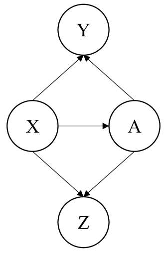
Figure 1: Graphical model of the probabilistic neural network with IB-inspired spatial attention mechanism (§3.2).

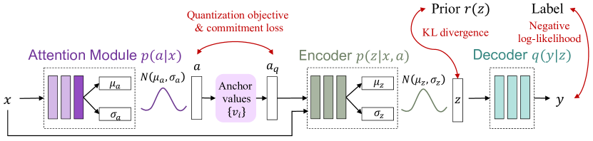
Figure 2: Framework of the IB-inspired spatial attention mechanism for visual recognition. The input $x$ is passed through an attention module to produce a continuous variational attention map $a$, which is quantized to a discrete attention map $a_{q}$ using a set of learnable anchor values $v_{i}$. Then, $a_{q}$ and $x$ are encoded to a latent vector $z$, and decoded to a prediction $y$. Loss function in Eq. (10). See §3.2 and §3.3.

2.2 IB-Inspired Mask Generation

IB theory has been explored in tasks such as representation learning Alemi et al. (2017); Achille and Soatto (2018) and domain adaptation Du et al. (2020). Here, we focus on IB-inspired mask generation methods, which yield additive Schulz et al. (2019) or multiplicative masks Achille and Soatto (2018); Taghanaki et al. (2019); Zhmoginov et al. (2019) to restrict the information that flows to the successive layers.

Information Dropout Achille and Soatto (2018) multiplies the layer feature with a learnable noise mask to control the flow of information. This is equivalent to optimizing a modified cost function that approximates the IB Lagrangian of Tishby et al. (1999), allowing the learning of a sufficient, minimal and invariant representation for classification tasks. InfoMask Taghanaki et al. (2019) filters out irrelevant background signals using the masks optimized on IB theory, which improves the accuracy of localizing chest disease. Zhmoginov et al. Zhmoginov et al. (2019) generates IB-inspired Boolean attention masks for image classification models to completely prevent the masked-out pixels from propagating any information to the model output. Schulz et al. Schulz et al. (2019) adopts the IB concept for interpreting the decision-making of a pre-trained neural network, by adding noise to intermediate activation maps to restrict and quantify the flow of information. The intensity of the noise is optimized to minimize the information flow while maximizing the classification score.

In this paper, we propose an IB-inspired spatial attention mechanism based on a new variational approximation of the IB principle derived from a neural network incorporated with attention module ($\mathcal{L}_{\text{AttVIB}}$ in Eq. (17)). Compared with the above works, our optimization objective is not derived from the original IB Lagrangian of Tishby et al. (1999), thus the resulted attention mechanism is parameterized with different network architectures. Besides, we focus on learning continuous spatial attention instead of noise masks Achille and Soatto (2018); Schulz et al. (2019), which is also different from the Boolean attention in Zhmoginov et al. (2019).

3 Methodology

3.1 Overview

We derived the framework of the proposed spatial attention mechanism theoretically from the IB principle on a neural network incorporated with an attention module. Assuming that random variables $X,Y,A$ and $Z$ follow the joint conditional distribution of the model shown in Fig. 6. Here, $X,Y,A$ and $Z$ denote the input, output, spatial attention map, and the latent representation obtained from $X$ and $A$, respectively. We drive the proposed spatial attention framework based on the joint distribution and the IB principle. The resulted framework is shown in Fig. 2, which consists of an attention module $p(a|x)$, a set of anchor values $\{v_{i}\}$ for quantization, an encoder $p(z|x,a)$, and a decoder $q(y|z)$.

The input $x$ is first passed through the attention module $p(a|x)$ to produce a continuous variational attention map $a$, which is quantized to a discrete attention map $a_{q}$ using a set of learnable anchor values $v_{i}$. Then, $a_{q}$ and $x$ are encoded to a latent vector $z$, and decoded to a prediction $y$. The whole framework is trained end-to-end using the loss function defined in Eq. (10). The derivation of the framework is shown in §3.2, and more details are provided in the supplementary. The attention score quantization process is shown in §3.3.

3.2 IB-inspired Spatial Attention Mechanism

We introduce the IB principle Tishby et al. (1999) to learn the spatial attention that minimizes the MI between the masked representation and the input, while maximizing the MI between the masked representation and the class label. Different from Alemi et al. (2017) for a standard learning framework, we derive new variational bounds of MI within an attentive framework for visual recognition, which lead to an IB-inspired spatial attention mechanism.

Let the random variables $X,Y,A$ and $Z$ denote the input, output, spatial attention map, and the latent representation obtained from $X$ and $A$, respectively. The MI between the latent feature $Z$ and its output $Y$ is defined as:

$$I(Z;Y)=\int p(y,z)\log\frac{p(y|z)}{p(y)}dydz.$$ (1)

We introduce $q(y|z)$ to be a variational approximation of the intractable $p(y|z)$. Since the Kullback Leibler (KL) divergence is always non-negative, we have:

$$\begin{split}&D_{\text{KL}}[p(y|z)||q(y|z)]=\int p(y|z)\log\frac{p(y|z)}{q(y|z)}dy\geq 0\\ &\Rightarrow\int p(y|z)\log p(y|z)dy\geq\int p(y|z)\log q(y|z)dy,\end{split}$$ (2)

which leads to

$$I(Z;Y)\geq\int p(y,z)\log q(y|z)dydz+H(Y),$$ (3)

where $H(Y)\!=\!-\int p(y)\log p(y)dy$ is the entropy of $Y$, which is independent of the optimization procedure thus can be ignored. By leveraging the fact that $p(y,z)\!=\!\int p(x,y,z,a)dxda\!=\!\int p(x)p(a|x)p(y|x,a)p(z|x,a)dxda$ (see Fig. 6), and ignoring $H(Y)$, the new variational lower bound is as follows:

where $p(a|x)$ is the attention module, $p(z|x,a)$ is the encoder, and $q(y|z)$ is the decoder. $I(Z;Y)$ can thus be maximized by maximizing its variational lower bound.

Next, to minimize the MI between the attention-modulated representation and the input, we consider $I(Z;X,A)$, and obtain the following upper bound:

where $r(z)$ is a prior distribution of $z$. In our experiments, we use a spherical Gaussian $\mathcal{N}(z|0,I)$ as the prior $r(z)$.

By combining Eq. (14) and (15), we obtain the lower bound of the attentive variational information bottleneck:

$$\begin{split}\mathcal{L}_{\text{AttVIB}}&\equiv I(Z;Y)-\beta I(Z;X,A)\\ =\int&p(x,y)p(a|x)p(z|x,a)\log q(y|z)dxdadydz\\ -\beta&\int p(x)p(a|x)p(z|x,a)\log\frac{p(z|x,a)}{r(z)}dxdadz,\end{split}$$ (6)

which offers an IB-inspired spatial attention mechanism for visual recognition. Here, $\beta\!>\!0$ controls the tradeoff between information compression and prediction accuracy.

We approximate $p(x)$, $p(x,y)$ with empirical distribution $p(x)\!=\!\frac{1}{N}\sum_{n=1}^{N}\delta_{x_{n}}(x)$, $p(x,y)\!=\!\frac{1}{N}\sum_{n=1}^{N}\delta_{x_{n}}(x)\delta_{y_{n}}(y)$ following Alemi et al. (2017), where $N$ is the number of training samples, $x_{n}$ and $(x_{n},y_{n})$ are samples drawn from data distribution $p(x)$ and $p(x,y)$, respectively. The approximated lower bound $\mathcal{L}_{\text{AttVIB}}$ can thus be written as:

Similar to Alemi et al. (2017), we suppose to use the attention module of the form $p(a|x)\!=\!\mathcal{N}(a|g_{e}^{\mu}(x),g_{e}^{\Sigma}(x))$, and the encoder of the form $p(z|x,a)\!=\!\mathcal{N}(z|f_{e}^{\mu}(x,a),f_{e}^{\Sigma}(x,a))$, where $g_{e}$ and $f_{e}$ are network modules. To enable back-propagation, we use the reparametrization trick Kingma and Welling (2014), and write $p(a|x)da\!=\!p(\varepsilon)d\varepsilon$ and $p(z|x,a)dz\!=\!p(\epsilon)d\epsilon$, where $a\!=\!g(x,\varepsilon)$ and $z\!=\!f(x,a,\epsilon)$ are deterministic functions of $x$ and the Gaussian random variables $\varepsilon$ and $\epsilon$. The loss function is:

The first term of the loss function is the negative log-likelihood of the prediction, where the label $y_{n}$ of $x_{n}$ is predicted from the latent encoding $z$, and $z$ is generated from $x_{n}$ and its attention map $a\!=\!g(x_{n},\varepsilon)$. Minimizing this term leads to maximal prediction accuracy. The second term is the KL divergence between distributions of latent encoding $z$ and the prior $r(z)$, the minimization of which enables the model to learn an IB-inspired spatial attention mechanism for visual recognition. This is different from the regular IB principle Tishby et al. (1999); Alemi et al. (2017) which is only for the representation learning without attention module.

	Image Class.		Fine-grained Recog.		Cross-domain Class.
Model	CIFAR-10	CIFAR-100	CUB-200-2011	SVHN	STL10-train	STL10-test
– Existing architectures –
VGG Simonyan and Zisserman (2015)	7.77	30.62	34.64	4.27	54.66	55.09
VGG-GAP Zhou et al. (2016)	9.87	31.77	29.50	5.84	56.76	57.24
VGG-PAN Seo et al. (2018)	6.29	24.35	31.46	8.02	52.50	52.79
VGG-DVIB Alemi et al. (2017)	4.64∗	22.88∗	23.94∗	3.28∗	51.40∗	51.60∗
WRN Zagoruyko and Komodakis (2016)	4.00	19.25	26.50	–	–	–
– Architectures with attention –
VGG-att2 Jetley et al. (2018)	5.23	23.19	26.80	3.74	51.24	51.71
VGG-att3 Jetley et al. (2018)	6.34	22.97	26.95	3.52	51.58	51.68
WRN-ABN Fukui et al. (2019)	3.92∗	18.12	–	2.88∗	50.90∗	51.24∗
VGG-aib (ours)	4.28	21.56	23.73	3.24	50.64	51.24
VGG-aib-qt (ours)	4.10	20.87	21.83	3.07	50.44	51.16
WRN-aib (ours)	3.60	17.82	17.26	2.76	50.08	50.84
WRN-aib-qt (ours)	3.43	17.64	15.50	2.69	50.34	50.49

Table 1: Top-1 error for image classification (§4.1), fine-grained recognition (§4.2), and cross-dataset classification (§4.3). ^∗ denotes re-implementation or re-training. Other values are from the original paper. Best values of different backbones are in bold.

3.3 Attention Score Quantization

We define the continuous attention space as $A\!\in\!\mathbb{R}^{W_{a}\!\times\!H_{a}}$, and the quantized attention space as $A_{q}\!\in\!\mathbb{R}^{W_{a}\!\times\!H_{a}}$, where $W_{a},H_{a}$ are the width and height of the attention map, respectively. As shown in Fig. 2, the input $x$ is passed through an attention module to produce a continuous variational attention map $a$, which is mapped to a discrete attention map $a_{q}$ through a nearest neighbour look-up among a set of learnable anchor values $\{v_{i}\!\in\!\mathbb{R}\}_{i=1}^{Q}$, which is given by:

$$a_{q}^{(w,h)}=v_{k},\;k=\arg\min_{j}\|a^{(w,h)}-v_{j}\|_{2},$$ (9)

where $w\!=\!1\dots W_{a},h\!=\!1\dots H_{a}$ are spatial indices. In this way, each score $a^{(w,h)}$ in the continuous attention map is mapped to the 1-of-$Q$ anchor value. The quantized attention map $a_{q}$ and the input $x$ are then encoded into a latent representation $z\!\in\!\mathbb{R}^{K}$, where $K$ is the dimension of the latent space. Finally, $z$ is mapped to the prediction probabilities $y\!\in\!\mathbb{R}^{C}$, and $C$ is the number of classes. The complete model parameters include the parameters of the attention module, encoder, decoder, and the anchor values $\{v_{i}\!\in\!\mathbb{R}\}_{i=1}^{Q}$.

As the $\arg\min$ operation in Eq. (9) is not differentiable, we resort to the straight-through estimator Bengio et al. (2013) and approximate the gradient of $a_{q}$ using the gradients of $a$. Though simple, this estimator worked well for the experiments in this paper. To be concrete, in the forward process the quantized attention map $a_{q}$ is passed to the encoder, and during the backwards computation, the gradient of $a$ is passed to the attention module unaltered. Such a gradient approximation makes sense because $a_{q}$ and $a$ share the same $W_{a}\!\times\!H_{a}$ dimensional space, and the gradient of $a$ can provide useful information on how the attention module could change its output to minimize the loss function defined in Eq. (19).

The overall loss function is thus defined as in Eq. (10), which extends Eq. (19) with two terms, namely a quantization objective $\|\text{sg}[g(x_{n},\varepsilon)]\!-\!a_{q}^{\varepsilon}\|_{2}^{2}$ weighted by $\lambda_{q}$, and a commitment term $\|g(x_{n},\varepsilon)\!-\!\text{sg}[a_{q}^{\varepsilon}]\|_{2}^{2}$ weighted by $\lambda_{c}$, where $\text{sg}[\cdot]$ is the stopgradient operator Van Den Oord et al. (2017), and $a_{g}^{\varepsilon}$ is the quantized version of $a\!=\!g(x_{n},\varepsilon)$. The former updates the anchor values to move towards the attention map $a$, and the latter forces the attention module to commit to the anchor values. We set $\beta\!=0.01$, $\lambda_{g}\!=\!0.4$, and $\lambda_{c}\!=\!0.1$ empirically.

$$\begin{split}\mathcal{L}\!=\!-&\frac{1}{N}\sum_{n=1}^{N}\!\{\mathbb{E}_{\epsilon\sim p(\epsilon)}[\mathbb{E}_{\varepsilon\sim p(\varepsilon)}[\log q(y_{n}|f(x_{n},a_{q}^{\varepsilon},\epsilon))]]\\ +&\mathbb{E}_{\varepsilon\sim p(\varepsilon)}[\beta D_{\text{KL}}[p(z|x_{n},a_{q}^{\varepsilon})\parallel r(z)]\\ +\lambda_{q}&\|\text{sg}[g(x_{n},\varepsilon)]\!-\!a_{q}^{\varepsilon}\|_{2}^{2}\!+\!\lambda_{c}\|g(x_{n},\varepsilon)\!-\!\text{sg}[a_{q}^{\varepsilon}]\|_{2}^{2}]\}.\end{split}$$ (10)

An illustration of the whole framework is shown in Fig. 2. In practice, we first use an feature extractor, e.g.VGGNet Simonyan and Zisserman (2015), to extract an intermediate feature $f$ from the input $x$, then learn the attention $a,a_{q}$ and the variational encoding $z$ from $f$ instead of $x$.

Model	Spatial	CIFAR-10				CIFAR-100				Frequency	CIFAR-10	CIFAR-100
		$p\!=\!4$	$p\!=\!8$	$p\!=\!12$	$p\!=\!16$	$p\!=\!4$	$p\!=\!8$	$p\!=\!12$	$p\!=\!16$
VGG-att3∗	color	91.46	79.61	37.71	7.12	52.92	39.93	25.40	14.56	$r\!>\!4$	83.06	3.69
	svhn	90.97	75.70	36.74	6.51	82.08	63.16	39.07	21.03	$r\!<\!12$	49.61	50.90
VGG-aib	color	99.22	99.69	93.78	20.59	98.88	98.56	95.92	22.70	$r\!>\!4$	99.91	99.78
	svhn	98.59	97.52	97.35	72.86	98.73	96.70	96.69	93.02	$r\!<\!12$	53.26	79.13
VGG-aib-qt	color	99.26	99.79	91.10	18.36	99.18	99.30	94.59	20.54	$r\!>\!4$	99.96	99.60
	svhn	98.65	98.04	97.85	78.82	99.12	97.64	97.21	94.79	$r\!<\!12$	73.52	79.70
WRN-ABN	color	90.76	65.01	33.89	13.24	89.74	61.38	30.56	9.67	$r\!>\!4$	38.14	14.04
	svhn	90.40	68.41	38.46	16.55	92.77	63.67	30.57	9.47	$r\!<\!12$	36.33	25.43
WRN-aib	color	99.95	93.94	45.17	6.69	99.86	95.35	64.27	17.15	$r\!>\!4$	78.96	90.44
	svhn	99.94	97.34	81.98	47.65	99.90	97.77	89.37	62.64	$r\!<\!12$	84.58	94.18
WRN-aib-qt	color	99.84	84.18	28.94	4.64	99.97	97.07	69.51	25.80	$r\!>\!4$	72.05	94.13
	svhn	99.91	96.05	70.75	28.35	99.95	98.52	89.00	63.10	$r\!<\!12$	76.53	93.17

Table 2: Interpretability scores under spatial and frequency domain modification on CIFAR-10 and CIFAR-100. $p$ is the window size of the modified region. $r$ is the radius in frequency domain. See §4.4 for more details. ^∗ denotes re-implementation. Best values in bold.

4 Experiments

To demonstrate the effectiveness of the proposed IB-inspired spatial attention, we conduct extensive experiments on various visual recognition tasks, including image classification (§4.1), fine-grained recognition (§4.2), and cross-dataset classification (§4.3), and achieve improved performance over baseline models. In §4.4, we compare the interpretability of our attention maps with those of other attention models both qualitatively and quantitatively. We conduct an ablation study in §4.5. More details are shown in the supplementary.

4.1 Image Classification

Datasets and models. CIFAR-10 Krizhevsky et al. (2009) contains $60,000$ $32\!\times\!32$ natural images of $10$ classes, which are splited into $50,000$ training and $10,000$ test images. CIFAR-100 Krizhevsky et al. (2009) is similar to CIFAR-10, except that it has $100$ classes. We extend standard architectures, VGG and wide residual network (WRN), with the proposed IB-inspired spatial attention, and train the whole framework from scratch on CIFAR-10, and CIFAR-100, respectively. We use original input images after data augmentation (random flipping and cropping with a padding of 4 pixels).

Results on CIFAR. As shown in Table 1, the proposed attention mechanism achieves noticeable performance improvement over standard architectures and existing attention mechanisms such as GAP, PAN, VGG-att and ABN. To be specific, VGG-aib achieves $3.49\%$ and $9.06\%$ decrease of errors over the baseline VGG model on CIFAR-10 and CIFAR-100, respectively. The quantized attention model VGG-aib-qt further decreases the errors over VGG-aib by $0.18\%$ and $0.69\%$ on the two datasets. Compared with other VGG-backboned attention mechanisms, ours also achieve superior classification performances. Similarly, WRN-aib and WRN-aib-qt also decrease the top-1 errors on CIFAR-10 and CIFAR-100.

4.2 Fine-grained Recognition

Datasets and models. CUB-200-2011 (CUB) Wah et al. (2011) contains $5,994$ training and $5,794$ testing bird images from $200$ classes. SVHN collects $73,257$ training, $26,032$ testing, and $531,131$ extra digit images from house numbers in street view images. For CUB, we perform the same preprocessing as Jetley et al. (2018). For SVHN, we apply the same data augmentation as CIFAR.

Results on CUB. The proposed VGG-aib and VGG-aib-qt achieves smaller classification error compared with baselines built on VGG, including GAP, PAN, and VGG-att. Specially, VGG-aib and VGG-aib-qt outperform VGG-att for a $3.07\%$ and $4.97\%$, respectively.

Results on SVHN. Our proposed method achieves lower errors with VGG-backboned models, and comparative errors for WRN backbone methods.

4.3 Cross-domain Classification

Datasets and models. STL-10 contains $5,000$ training and $8,000$ test images of resolution $96\!\times\!96$ organized into $10$ classes. Following Jetley et al. (2018), the models trained on CIFAR-10 are directly tested on STL-10 training and test sets without finetuning to verify the generalization abilities.

Results on STL-10. As shown in Table 1, the proposed attention model outperforms other competitors on VGG backbone, and achieves comparative performance for WRN backbone.

4.4 Interpretability Analysis

An interpretable attention map is expected to faithfully highlight the regions responsible for the model decision. Thus, an interpretable attention mechanism is expected to yield consistent attention maps for an original input and a modified input if the modification does not alter the model decision. Here, we quantify the interpretability of an attention mechanism by calculating the ‘interpretability score’, i.e. the percentage of attention-consistent samples in prediction-consistent samples under modifications in the spatial or frequency domain. Here, the attention consistency is measured by the cosine similarity between two flattened and normalized attention maps.

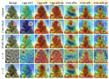
Figure 3: Visualization of attention maps for interpretability (§4.4).

The spatial domain modification includes randomly occluding the original images in CIFARs with color blocks or images drawn from distinct datasets. The size of the modified region $p$ ranges from $4$ to $16$. The $2$nd and $3$rd rows in Fig. 3 show exemplar images occluded by a random color block and an image randomly drawn from SVHN, respectively, where $p\!=\!8$. As can be observed, our spatial attention model VGG-aib(-qt), and WRN-aib(-qt) yield consistent attention maps with the original images (first row). The interpretability scores are listed in Table 2. Our method consistently outperforms other spatial attention mechanisms with the same backbone by a large margin on two datasets for various $p$. This is because the IB-inspired attention mechanism minimizes the MI between the attention-modulated features and the inputs, thus mitigating the influence of ambiguous information exerted on the inputs to some extent.

We also conduct frequency domain modification, which is done by performing Fourier transform on the original samples, and feeding only high-/low-frequency (HF/LF) components into the model. To preserve enough information and maintain the classification performance, we focus on HF components of $r\!>\!4$, and LF components of $r\!<\!12$, where $r$ is the radius in frequency domain defined as in Wang et al. (2020). The $4$th and $5$th rows in Fig. 3 show exemplar images constructed from HF and LF components, respectively. Our attention maps are more royal to those of the original images compared with other competitors. Out method also yields much better quantitative results than other attention models, as illustrated in Table 2. This is because our IB-inspired attention mechanism can well capture the task-specific information in the input by maximizing the MI between the attention-modulated feature and the task output, even when part of the input information is missing.

4.5 Ablation Study

We conduct ablation studies on CIFAR-10 with the VGG backbone to assess the effectiveness of each component.

Effectiveness of attention module. Table 1 shows that VGG-aib and VGG-aib-qt outperform the IB-based representation learning model VGG-DVIB.

Information tradeoff. $\beta$ controls the amount of information flow that bypasses the bottleneck of the network. To measure the influence of $\beta$ on the performance, we plot the accuracy values with varying $\beta$ in Fig. 4 (a). As can be observed, the accuracy is largest when $\beta\!=\!0.01$.

Latent vector dimension. We experiment on $K\!=\!64,128$, $256,512$, $1024$. As shown in Fig. 4 (b), $K\!=\!256$ achieves the best performance.

Attention score quantization. Fig. 4 (c) shows the classification accuracy when varying number of anchor values $Q$, where $Q$ between $20$ and $50$ gives better performance. Exemplary attention maps of cases that are wrongly classified by VGG-aib but are correctly predicted by VGG-aib-qt are listed in Fig. 5. As can be observed, attention quantization can further help focus on more concentrated regions with important information, thus improve the prediction accuracy.

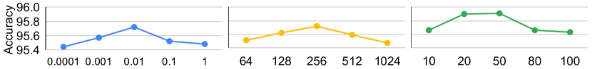
Figure 4: Ablation study on CIFAR-10 with VGG backbone (§4.5).

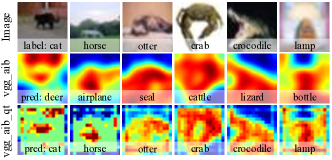
Figure 5: Effect of attention score quantization. See §4.5 for details.

5 Conclusion

We propose a spatial attention mechanism based on IB theory for generating probabilistic maps that minimizes the MI between the masked representation and the input, while maximizing the MI between the masked representation and the task label. To further restrict the information bypassed by the attention map, we incorporate an adaptive quantization mechanism to regularize the attention scores by rounding the continuous scores to the nearest anchor value during training. Extensive experiments show that the proposed IB-inspired spatial attention mechanism significantly improves the performance for visual recognition tasks by focusing on the most informative parts of the input. The generated attention maps are interpretable for the decision making of the DNNs, as they consistently highlight the informative regions for the original and modified inputs with the same semantics.

In this supplementary, we first present the detailed deriviation of the proposed spatial attention mechanism inspired by the Information Bottleneck (IB) tishby1999information principle. We then provide explanation of the recognition tasks in our experiments. Finally, we show the implementation details of our model.

Appendix A Deriviation of the IB-inspired Spatial Attention

In this section, we present the detailed deriviation of the variational lowerbound of the attentive variational information bottleneck $\mathcal{L}_{\text{AttVIB}}\!\equiv\!I(Z;Y)\!-\!\beta I(Z;X,A)$.

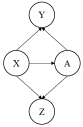
Figure 6: Graphical model of the probabilistic neural network with IB-inspired spatial attention mechanism.

A.1 Lowerbound of $I(Z;Y)$

Let the random variables $X,Y,A$ and $Z$ denote the input, output, the spatial attention map, and the latent representation obtained from $X$ and $A$, respectively. The MI between the latent feature $Z$ and its output $Y$ is defined as:

$$I(Z;Y)=D_{\text{KL}}[p(y,z)||p(y)p(z)]=\int p(y,z)\log\frac{p(y,z)}{p(y)p(z)}dydz=\int p(y,z)\log\frac{p(y|z)}{p(y)}dydz.$$ (11)

We introduce $q(y|z)$ to be a variational approximation of the intractable $p(y|z)$. Since the Kullback Leibler (KL) divergence is always non-negative, we have:

$$D_{KL}[p(Y|Z)||q(Y|Z)]=\int p(y|z)\log\frac{p(y|z)}{q(y|z)}dy\geq 0\Rightarrow\int p(y|z)\log p(y|z)dy\geq\int p(y|z)\log q(y|z)dy,$$ (12)

which leads to

$$I(Z;Y)\!\geq\!\int p(y,z)\!\log\frac{q(y|z)}{p(y)}dydz\!=\!\int p(y,z)\!\log q(y|z)dydz\!-\!\int p(y)\log p(y)dy\!=\!\int p(y,z)\!\log q(y|z)dydz\!+\!H(Y),$$ (13)

where $H(Y)\!=\!-\int p(y)\log p(y)dy$ is the entropy of $Y$ , which is independent of the optimization procedure thus can be ignored. By leveraging the fact that $p(y,z)\!=\!\int p(x,y,z,a)dxda\!=\!\int p(x)p(a|x)p(y|x,a)p(z|x,a)dxda$ (see Fig. 6), and ignoring $H(Y)$, the new variational lower bound is as follows:

$$I(Z;Y)\geq\int p(x,y)p(a|x)p(z|x,a)\log q(y|z)dxdadydz,$$ (14)

where $p(a|x)$ is the attention module, $p(z|x,a)$ is the encoder, and $q(y|z)$ is the decoder where $z$ is the output of $p(z|x,a)$. $I(Z;Y)$ can thus be maximized by maximizing its variational lower bound.

A.2 Upperbound of $I(Z;X,A)$

Next, to minimize the MI between the masked repsentation and the input, we consider $I(Z;X,A)$, and obtain the following upper bound according to the chain rule for mutual information, which is calculated as follows:

$$\begin{split}I(Z;X,A)=&I(Z;X)+I(Z;A|X)=\int p(x,z)\log\frac{p(x,z)}{p(x)p(z)}dxdz+\int p(x,a,z)\log\frac{p(x)p(x,a,z)}{p(x,a)p(x,z)}dxdadz\\ \leq&\int p(x,z)\log\frac{p(z|x)}{r(z)}dxdz+\int p(x,a,z)\log\frac{p(z|x,a)}{p(z|x)}dxdadz\end{split}$$ (15)

where $r(z)$ is a prior distribution of $z$. This inequation is also from the nonnegativity of the Kullback Leibler (KL) divergence.

Eq. (15) can be further simplified as follows:

$$\begin{split}&I(Z;X,A)\leq\int p(x,z)\log\frac{p(z|x)}{r(z)}dxdz+\int p(x,a,z)\log\frac{p(z|x,a)}{p(z|x)}dxdadz\\ =&\int p(x)p(z|x)\log\frac{p(z|x)}{r(z)}dxdz+\int p(x)p(a|x)p(z|x,a)\log\frac{p(z|x,a)}{p(z|x)}dxdadz\\ =&\int p(x)p(z|x)(\int p(a|z,x)da)\log\frac{p(z|x)}{r(z)}dxdz+\int p(x)p(a|x)p(z|x,a)\log\frac{p(z|x,a)}{p(z|x)}dxdadz\\ =&\int p(x)p(a,z|x)\log\frac{p(z|x)}{r(z)}dxdadz+\int p(x)p(a|x)p(z|x,a)\log\frac{p(z|x,a)}{p(z|x)}dxdadz\\ =&\int p(x)p(a|x)p(z|x,a)\log\left(\frac{p(z|x,a)}{p(z|x)}\frac{p(z|x)}{r(z)}\right)dxdadz=\int p(x)p(a|x)p(z|x,a)\log\frac{p(z|x,a)}{r(z)}dadz\end{split}$$ (16)

By combining the two bounds in Eq. (14) and (16), we obtain the attentive variational information bottleneck:

$$\begin{split}\mathcal{L}_{\text{AttVIB}}&\equiv I(Z;Y)-\beta I(Z;X,A)\\ =\int&p(x,y)p(a|x)p(z|x,a)\log q(y|z)dxdadydz-\beta\int p(x)p(a|x)p(z|x,a)\log\frac{p(z|x,a)}{r(z)}dxdadz,\end{split}$$ (17)

which offers an IB-inspired spatial attention mechanism for visual recognition.

Following alemi2017deep, we approximate $p(x)$ and $p(x,y)$ with empirical data distribution $p(x)=\frac{1}{N}\sum_{n=1}^{N}\delta_{x_{n}}(x)$ and $p(x,y)=\frac{1}{N}\sum_{n=1}^{N}\delta_{x_{n}}(x)\delta_{y_{n}}(y)$, where $N$ is the number of training samples, $x_{n}$ and $(x_{n},y_{n})$ are samples drawn from data distribution $p(x)$ and $p(x,y)$, respectively. The approximated lower bound $\mathcal{L}_{\text{AttVIB}}$ can thus be written as:

$$\widetilde{\mathcal{L}}_{\text{AttVIB}}=\frac{1}{N}\sum_{n=1}^{N}\{\int p(a|x_{n})p(z|x_{n},a)\log q(y_{n}|z)dadz-\beta\int p(a|x_{n})p(z|x_{n},a)\log\frac{p(z|x_{n},a)}{r(z)}dadz\}.$$ (18)

Similar to alemi2017deep, we suppose to use the attention module of the form $p(a|x)\!=\!\mathcal{N}(a|g_{e}^{\mu}(x),g_{e}^{\Sigma}(x))$, and the encoder of the form $p(z|x,a)\!=\!\mathcal{N}(z|f_{e}^{\mu}(x,a),f_{e}^{\Sigma}(x,a))$, where $g_{e}$ and $f_{e}$ are network modules. To enable back-propagation, we use the reparametrization trick kingma2014auto, and write $p(a|x)da\!=\!p(\varepsilon)d\varepsilon$ and $p(z|x,a)dz\!=\!p(\epsilon)d\epsilon$, where $a\!=\!g(x,\varepsilon)$ and $z\!=\!f(x,a,\epsilon)$ are deterministic functions of $x$ and the Gaussian random variables $\varepsilon$ and $\epsilon$. The final loss function is:

$$\mathcal{L}\!=\!-\frac{1}{N}\sum_{n=1}^{N}\!\{\mathbb{E}_{\epsilon\sim p(\epsilon)}[\mathbb{E}_{\varepsilon\sim p(\varepsilon)}[\log q(y_{n}|f(x_{n},g(x_{n},\varepsilon),\epsilon))]]+\beta\mathbb{E}_{\varepsilon\sim p(\varepsilon)}[D_{KL}[p(z|x_{n},g(x_{n},\varepsilon))\parallel r(z)]]\}.$$ (19)

The first term is the negative log-likelihood of the prediction, where the label $y_{n}$ of $x_{n}$ is predicted from the latent encoding $z$, and $z$ is generated from the $x_{n}$ and the attention $a=g(x_{n},\varepsilon)$. Minimizing this term leads to maximal prediction accuracy. The second term is the KL divergence between distributions of latent encoding $z$ and the prior $r(z)$. The minimization of the KL terms in Eq. (19) enables the model to learn an IB-inspired spatial attention mechanism for visual recognition.

Appendix B Introduction of the recognition tasks

Fine-grained recognition is to differentiate similar subordinate categories of a basic-level category, e.g. bird species WahCUB_200_2011, flower types nilsback2008automated, dog breeds khosla2011novel, automobile models krause20133d, etc.  The annotations are usually provided by domain experts who are able to distinguish the subtle differences among the highly-confused sub-categories. Compared with generic image classification task, fine-grained recognition would benefit more from finding informative regions that highlight the visual differences among the subordinate categories, and extracting discriminative features therein.

Cross-domain classification is to test the generalization ability of a trained classifier on other domain-shifted benchmarks, i.e. datasets that have not been used during training. In our experiments, we directly evaluate the models trained on CIFAR-10 on the train and test set of STL-10 following jetley2018learn.

Appendix C Implementation details

Network Configuration. For CIFAR and SVHN, the feature extractor consists of the first three convolutional blocks of VGG, where the max-pooling layers are omitted, or the first two residual blocks of WRN. In VGG-aib, $g_{e}^{\mu}$ for obtaining the $\mu_{a}$ is built as: Conv($3\!\times\!3,1$) $\rightarrow$ Sigmoid, and $\sigma_{a}$ is calculated from $\mu_{a}$ through a Conv($1\!\times\!1,1$), which is inspired by bahuleyan2018variational. In WRN-aib, $g_{e}^{\mu}$ contains an extra residual block compared with that in VGG backbone, and $\sigma_{a}$ is obtained in the same way. The encoder contains the remaining convolutional building blocks from VGG or WRN, with an extra FC layer that maps the flattened attention-modulated feature to a $2K$ vector, where the first $K$-dim is $\mu$, and the remaining $K$-dim is $\sigma$ (after a softplus activation). The decoder maps the sampled latent representation $z$ to the prediction $y$, which is built as: FC($K\!\times\!K$) $\rightarrow$ReLU$\rightarrow$FC($K\!\times\!C$) for VGG backbone, and ReLU$\rightarrow$FC($K\!\times\!C$) for WRN backbone, where $K$ is the dimension of the latent encoding, and $C$ is the number of classes. For CUB, the feature extractor is built from the whole convolutional part of VGG. The encoder only contains a Linear layer. The structure of the attention module and the decoder is the same as above. For VGG-aib-qt and WRN-aib-qt, the number of anchor values $Q$ are $20$ and $50$, respectively. The values $\{v_{i}\}$ are initialized by evenly dividing $[0,1]$ and then trained end-to-end within the framework.

Comparions of #parameters. In Table. 3, we report the number of parameters for different attention mechanisms under various settings. We will add this to the future version.

Table 3: Comparisons of the number of parameters (M).

Input Size	#Class	VGG-att3	VGG-aib	VGG-aib-qt	WRN-ABN	WRN-aib	WRN-aib-qt
$32\!\times\!32$,	10	19.86	20.05	20.05	64.35	65.00	65.00
$32\!\times\!32$,	100	19.99	20.07	20.07	64.48	65.11	65.11
$224\!\times\!224$,	200	-	24.28	24.28	-	130.73	130.73

Hyper-parameter selection. We first determine the ranges of the hyper-parameters by referring to related works alemi2017deep,van2017neural, and then discover the best ones through experiments. Following this scheme, we choose a good $\beta$ for different backbones by experimenting on $\beta\!=\!10^{-p},p=0,\dots,4$. For a certain backbone, the hyper-parameters are the same for tasks whose inputs share the same resolution. The hyper-parameters varied slightly for different backbones. Latent vector dimension $K$ defines the size of the bottleneck as in alemi2017deep, which does not necessarily match the latent dimension of other architectures.

Training. Models are trained from scratch except on CUB following jetley2018learn. We use an SGD optimizer with weight decay $5\times 10^{-4}$ and momentum $0.9$, and train for $200$ epochs in total. The batch size is $128$ for all the datasets. For VGG-aib(-qt), the initial learning rate is $0.1$, which is scaled by $0.5$ every $25$ epochs. For WRN-aib(-qt), the initial learning rate is $0.1$, and is multiplie,d by $0.3$ at the $60,120$ and $180$-th epoch.

Inference. We draw $4$ samples from $p(\varepsilon)$ for $a$ and $12$ samples from $p(\epsilon)$ for $z$ in the lower bound of the IB-inspired attention mechanism in Eq. (17) and the loss in Eq. (18).

Running time analysis. We show the FLOPs and inference time of our method in Table. 4.

Table 4: Running time analysis with various task settings.

Input Size	#Class	FLOPs (G)				Inference time per frame (ms)
		VGG-aib	VGG-aib-qt	WRN-aib	WRN-aib-qt	VGG-aib	VGG-aib-qt	WRN-aib	WRN-aib-qt
$32\!\times\!32$	10	3.79	3.79	39.14	39.14	3.43	3.68	8.53	8.55
$32\!\times\!32$	100	3.79	3.79	39.20	39.20	3.51	3.70	8.60	8.84
$224\!\times\!224$	200	16.75	16.75	50.97	50.97	3.58	3.81	10.47	10.66

Reproducibility. Our model is implemented using PyTorch and trained/tested on one Nvidia TITAN Xp GPU. To ensure reproducibility, our code is released at https://github.com/ashleylqx/AIB.git.

named varef

References

- Achille and Soatto [2018] Alessandro Achille and Stefano Soatto. Information dropout: Learning optimal representations through noisy computation. TPAMI, 40(12):2897–2905, 2018.
- Alemi et al. [2017] Alexander A Alemi, Ian Fischer, Joshua V Dillon, and Kevin Murphy. Deep variational information bottleneck. In ICLR, 2017.
- Bahdanau et al. [2015] Dzmitry Bahdanau, Kyunghyun Cho, and Yoshua Bengio. Neural machine translation by jointly learning to align and translate. In ICLR, 2015.
- Bengio et al. [2013] Yoshua Bengio, Nicholas Léonard, and Aaron Courville. Estimating or propagating gradients through stochastic neurons for conditional computation. arXiv preprint arXiv:1308.3432, 2013.
- Chorowski et al. [2015] Jan K Chorowski, Dzmitry Bahdanau, Dmitriy Serdyuk, Kyunghyun Cho, and Yoshua Bengio. Attention-based models for speech recognition. In NeurIPS, 2015.
- Du et al. [2020] Yingjun Du, Jun Xu, Huan Xiong, Qiang Qiu, Xiantong Zhen, Cees GM Snoek, and Ling Shao. Learning to learn with variational information bottleneck for domain generalization. In ECCV, 2020.
- Eriksen and Hoffman [1972] Charles W Eriksen and James E Hoffman. Temporal and spatial characteristics of selective encoding from visual displays. Perception & Psychophysics, 12(2):201–204, 1972.
- Fukui et al. [2019] Hiroshi Fukui, Tsubasa Hirakawa, Takayoshi Yamashita, and Hironobu Fujiyoshi. Attention branch network: Learning of attention mechanism for visual explanation. In CVPR, 2019.
- Han et al. [2020] Kai Han, Yunhe Wang, Hanting Chen, et al. A survey on visual transformer. arXiv preprint arXiv:2012.12556, 2020.
- Hu et al. [2018] Jie Hu, Li Shen, and Gang Sun. Squeeze-and-excitation networks. In CVPR, 2018.
- Hu et al. [2019] Han Hu, Zheng Zhang, Zhenda Xie, and Stephen Lin. Local relation networks for image recognition. In ICCV, 2019.
- Jetley et al. [2018] Saumya Jetley, Nicholas A Lord, Namhoon Lee, and Philip HS Torr. Learn to pay attention. In ICLR, 2018.
- Kingma and Welling [2014] Diederik P Kingma and Max Welling. Auto-encoding variational bayes. In ICLR, 2014.
- Koch and Ullman [1987] Christof Koch and Shimon Ullman. Shifts in selective visual attention: Towards the underlying neural circuitry. In Matters of Intelligence, pages 115–141. 1987.
- Koch et al. [2006] Kristin Koch, Judith McLean, et al. How much the eye tells the brain. Current Biology, 16(14):1428–1434, 2006.
- Krizhevsky et al. [2009] Alex Krizhevsky, Geoffrey Hinton, et al. Learning multiple layers of features from tiny images. 2009.
- Schulz et al. [2019] Karl Schulz, Leon Sixt, Federico Tombari, and Tim Landgraf. Restricting the flow: Information bottlenecks for attribution. In ICLR, 2019.
- Seo et al. [2018] Paul Hongsuck Seo, Zhe Lin, Scott Cohen, Xiaohui Shen, and Bohyung Han. Progressive attention networks for visual attribute prediction. In BMVC, 2018.
- Sharma et al. [2015] Shikhar Sharma, Ryan Kiros, and Ruslan Salakhutdinov. Action recognition using visual attention. In ICLR Workshop, 2015.
- Simonyan and Zisserman [2015] Karen Simonyan and Andrew Zisserman. Very deep convolutional networks for large-scale image recognition. In ICLR, 2015.
- Simonyan et al. [2013] Karen Simonyan, Andrea Vedaldi, and Andrew Zisserman. Deep inside convolutional networks: Visualising image classification models and saliency maps. arXiv preprint arXiv:1312.6034, 2013.
- Taghanaki et al. [2019] Saeid Asgari Taghanaki, Mohammad Havaei, Tess Berthier, Francis Dutil, Lisa Di Jorio, Ghassan Hamarneh, and Yoshua Bengio. Infomask: Masked variational latent representation to localize chest disease. In MICCAI, 2019.
- Tishby et al. [1999] Naftali Tishby, Fernando C Pereira, and William Bialek. The information bottleneck method. JMLR, 1999.
- Van Den Oord et al. [2017] Aaron Van Den Oord, Oriol Vinyals, et al. Neural discrete representation learning. In NeurIPS, 2017.
- Wah et al. [2011] C. Wah, S. Branson, P. Welinder, P. Perona, and S. Belongie. The Caltech-UCSD Birds-200-2011 Dataset. Technical report, 2011.
- Wang et al. [2020] Haohan Wang, Xindi Wu, Zeyi Huang, and Eric P Xing. High-frequency component helps explain the generalization of convolutional neural networks. In CVPR, 2020.
- Woo et al. [2018] Sanghyun Woo, Jongchan Park, Joon-Young Lee, and In So Kweon. Cbam: Convolutional block attention module. In ECCV, 2018.
- Xu et al. [2015] Kelvin Xu, Jimmy Ba, et al. Show, attend and tell: Neural image caption generation with visual attention. In ICML, 2015.
- Zagoruyko and Komodakis [2016] Sergey Zagoruyko and Nikos Komodakis. Wide residual networks. 2016.
- Zhmoginov et al. [2019] Andrey Zhmoginov, Ian Fischer, and Mark Sandler. Information-bottleneck approach to salient region discovery. In ICML Workshop, 2019.
- Zhou et al. [2016] Bolei Zhou, Aditya Khosla, Agata Lapedriza, Aude Oliva, and Antonio Torralba. Learning deep features for discriminative localization. In CVPR, 2016.