Universal quantum state preparation via revised greedy algorithm

Abstract

Preparation of quantum state lies at the heart of quantum information processing. The greedy algorithm provides a potential method to effectively prepare quantum states. However, the standard greedy algorithm, in general, cannot take the global maxima and instead becomes stuck on a local maxima. Based on the standard greedy algorithm, in this paper we propose a revised version to design dynamic pulses to realize universal quantum state preparation, i.e., preparing any arbitrary state from another arbitrary one. As applications, we implement this scheme to the universal preparation of single- and two-qubit state in the context of semiconductor quantum dots and superconducting circuits. Evaluation results show that our scheme outperforms the alternative numerical optimizations with higher preparation quality while possesses the comparable high efficiency. Compared with the emerging machine learning, it shows a better accessibility and does not require any training. Moreover, the numerical results show that the pulse sequences generated by our scheme are robust against various errors and noises. Our scheme opens a new avenue of optimization in few-level system and limited action space quantum control problems.

• April 2021

Keywords: Quantum state preparation, semiconductor double quantum dots, superconducting circuits, dynamic control pulses

1 Introduction

Benefited from the fascinating abilities afforded by the quantum mechanics, quantum computers of the future are supposed to tackle specific tasks that are intractable or even prohibitive to solve with their classical counterparts [1, 2, 3, 4, 5, 6, 7, 8]. Over the past few decades, a wide variety of physical modalities has been proposed theoretically and demonstrated experimentally to construct the prototypes of quantum computers, spanning from a single electron to the topological system [9, 10, 11, 12, 13, 14, 15, 16]. Along with the mature of the hardware, the task of designing control trajectory partially falls on the programming side which bridges quantum science and traditional disciplines.

It has been proved that with only arbitrary single-qubit rotations on the Bloch sphere plus an entangling two-qubit gate, arbitrary quantum logic can be performed on a gate-based quantum computer, or rather, they are universal [1]. Various scenarios have discussed how to decompose a quantum algorithm into an arrangement of these universal gates [1, 17, 18, 19]. Meanwhile, it has also been explored how to construct optimal gate synthesis with the universal gate set for general logical operation [20]. While, for a given experimental platform, there are always certain gates that are more efficient to implement than others, or even the key ingredients of the latter. Thus, they are often referred to as “native gates” of that platform. To enact quantum computation, it is required to decompose a given quantum algorithm into a sequence of discrete native gates according to the underlying hardware properties [21, 22].

Experimentally, these native gates are performed by electromagnetic pulses with precise amplitudes and durations. However, the difficulty of scheduling these pulses to implement a logical gate sharp increases with the decrease of the degrees of freedom in general. A prominent example is the pluses designing for a singlet-triplet ($S$-$T_{0}$) qubit in a semiconductor double quantum dot (DQD). Where the only tunable parameter is the exchange coupling between two trapped electrons, which associates with the rotation rate about the $z$-axis of the Bloch sphere. The process of designing pulses analytically requires to solve iteratively a set of nonlinear equations [23, 24, 25]. Thus it is a overhead costly and time-consuming task in practice. In order to improve efficiency, Ref. [26] discussed design pulses with supervised learning to get an approximation of that analytical solution. Considering the challenge to realize pulses with continuous intensity and duration in experiment, Ref. [27] employed deep reinforcement learning [28, 29, 30, 31] to explore the preparation of a specific state from another one with dynamic pulses whose intensity and duration are both discrete, yet at the expense of universality. Respecting the virtues of discrete control, Ref. [32] studied the preparation of a certain state from an arbitrary state. In contrast, Ref. [33] promised to prepare an arbitrary state from a specific state in a multi-level nitrogen-vacancy center system. It is a meaningful point that by combining Refs. [32] and [33] the driving between any states can be implemented as suggested in Ref. [32]. In addition, it is also a promising direction to train the network with both random initial state and target state to achieve the same objective directly. Except for the nascent machine learning, there are also several sophisticated versatile optimization approaches based on gradient can be utilized, such as stochastic gradient descent (SGD) [34], gradient ascent pulse engineering (GRAPE) [35, 36] and chopped random-basis optimization (CRAB) [37, 38]. They have been successfully applied to a wide array of optimization problems. While, suffering from the sensitivity to the initial control trajectory setting, in general, they can find only local maxima, instead of global maxima, and quit the iterative process with an inadequate fidelity.

In this paper, based on the standard greedy (SG) algorithm [39, 40], a common technology for optimization, we provide an improved version, i.e. revised greedy (RG) algorithm to drive an arbitrary state to another arbitrary state, or say, universal state preparation with discrete control. On the one hand, differing from the algorithms based on the machine learning, which suffers from the long hours of training and the resulting huge computational overhead, our scheme needs no training at all, which ensures a high accessibility. On the other hand, contrasting to the traditional optimization methods, our scheme overcomes the local optimality and achieves a higher preparing quality. In addition, compared with them, the average runtime of identifying the appropriate pulses with our scheme is comparable to the GRAPE, which is known for its high efficiency. We apply our scheme exemplarily to the universal single- and two-qubit state preparation in the context of $S$-$T_{0}$ spin qubits in semiconductor DQDs and superconducting quantum circuits Xmon qubits [41, 42]. Our method is general enough to be extended to varieties of few-level system and limited action space quantum control problems.

The remainder of this paper is organized as follows. In Sec. 2, we describe in detail the method used in this work. Then we present the results in the Sec. 3, and conclude in Sec. 4. The models considered in this paper are collected in Sec. 5.

2 Method

Dynamic programming, an important member of the optimization theory, divides a complex problem into multiple simple sub-problems, and then solves each sub-problem individually. It is expert in solving the Markov decision process, in which the resulting state $S^{\prime}$ is determined uniquely by the current state $S$ and the action $a$ taken by the agent while has no connection with the history of the system [43]. The SG algorithm, which is build upon the dynamic programming, approximates the global result by collecting the optimal solutions of each sub-problem [39, 40]. The SG algorithm as well as its variants is the most commonly used strategy to determine which action to explore in a given state in optimizations and acts as a crucial ingredient in many successful quantum control schemes, such as the designing of high-fidelity quantum gates [44, 45] and the scheduling of quantum gates to implement quantum algorithm [46]. However, because of the overemphasis on local optimality, in general, the SG algorithm cannot produce the global maxima. In order to overcome the local optimality of the SG algorithm, we propose here an revised version, i.e. RG algorithm to design the control pulses.

Our target is to design pulses to drive an arbitrary given quantum state to another arbitrary state. To illustrate the process of designing pulses clearly, we consider exemplarily the driving from the initial state $|S_{0}\rangle=|0\rangle$ to the target state $|S_{tar}\rangle=|1\rangle$ with single-parameter dynamic pulses. The quality of the state preparation is evaluated by the fidelity, which is defined as $F\equiv|\langle S_{tar}|S_{n}\rangle|^{2}$, where $|S_{n}\rangle$ (also noted as $S_{n}$ for simplicity) refers to the evolution state at time step $n$. The schematic of this processing is patterned in Fig. 1. To reduce the computational overhead, the control function is discretized as a piecewise constant (PWC) pulse-sequence [36]. The maximum evolution time $T$ is divided uniformly into $N$ slices with pulse duration $\mathrm{d}t=T/N$. All of the allowed actions adopted in this work accommodate the fundamental constraints and experimental realities, such as pulse height, duration, etc [47, 48, 49]. This control function can be readily implemented with suitable electrodes voltages generated by an arbitrary waveform generator in the platform of semiconductor QDs [50]. While, for the control of superconducting circuits, these pulses with discrete intensity and duration can be translated into continuous microwaves generated by a typical IQ modulation setup [49]. Presume there are four allowed actions $\{a^{1},a^{2},a^{3},a^{4}\}$ corresponding to four allowed pulse strengths respectively.

Figure 1: Schematic of the RG algorithm for control trajectory designing. The details of this algorithm are described in the main text of Sec. 2 and in the pseudocode Algor. 1.

The scheme goes as follows: initially, the fidelity of the state $S_{0}$ is $F_{0}=0$. Then, calculate each fidelity $F^{i}$ caused by the corresponding action $a^{i}$ after $\mathrm{d}t$ evolution. We assume these resulting fidelities are 0.1, 0.3, 0.2, 0.15 respectively, and all of them are bigger than $F_{0}$. Then we choose the maximum of $F^{i}$ as the fidelity at this time step, i.e. $F_{1}\leftarrow F^{2}=0.3$; the corresponding action as the “selected action”, $a_{0}\leftarrow a^{2}$; and the corresponding evolution state as the next state, $S_{1}\leftarrow S^{2}$. This step dovetails neatly with the SG algorithm: employ directly the “best action”. After, based on the state $S_{1}$, perform the allowed actions $a^{i}$ separately again and take the corresponding fidelities $F^{i}$. Assume the resulting fidelities are 0.26, 0.3, 0.28 and 0.25 respectively, and obviously there’s no new fidelity bigger than $F_{1}$. To overcome the local optimality in this case, we employ 3 strategies to decide which action should be selected: strategy 1, choose the “best action” according to the greedy algorithm; strategy 2, the “next-best action”; and strategy 3, the “worst action”. And repeat the above operations, until the final time step $N$ or the fidelity exceeds a certain satisfactory threshold. Note that in an episode, from the first step to the last, only one strategy is adopted to ensure the stability of the algorithm. Finally, take the action-sequence as the solution corresponding to the strategy in which we obtained the maximum fidelity. For current computer, with more than enough CPU cores available, these strategies can be readily executed on different processings in parallel, making it an extremely effective algorithm. The pseudocode of this RG algorithm is given in Algor. 1.

The core of this scheme lies at the introduction of deliberate perturbation, represented as the selection of “non-best” action, when the state are stuck on local maxima, which is regarded empirically as an efficient way to achieve a better performance [36]. This setting is necessary for cases like that: with the north pole of Bloch sphere targeted, the “best” action may always orient the state located in the equator along the equator and cannot reach a better place forever. In addition, unlike algorithms based on machine learning, there’s no training at all. Alternatively, the RG explores the suited action as well as the next state by trials and errors online, converting a complicated model-free environment into a simple model-based one which the algorithm fully understands [43]. So that it does not require learning of the environment and actions any more.

Our scheme achieves a better performance than the comparable approaches in few-level system and limited action space quantum control problems, such as the single- and two-qubit state preparation as we will demonstrate in the following section. Nonetheless, this advantage may diminish as the number of qubits and the action space blow up, partially due to the huge increase in them will limit this method’s efficiency. (For optimization problems with continuous action space, the machine learning certainly has more natural advantages.) In addition, in many-body preparation, such as the quantum state transfer, there may be a lack of a well metric to determine which state is “better” than others in the intermediate process. One possible route for improvement is to use this method in concert with other algorithms, which we leave as future works. However, even if the many-body state preparation is a very important topic from the application point of view, as we mentioned in the Introduction, with only arbitrary single- and two-qubit gates, any quantum logic can be implemented on a circuit-model quantum computer.

List of Algorithms 1 Pseudocode of the RG algorithm for control trajectory designing.

Initialize the time step $step=0$ and state $s_{step}$ according to the testing point.

Calculate the fidelity $F_{step}$ and make $F_{\mathrm{max}}=F_{0}=F_{step}$.

while True do

   Perform the allowed actions $a^{i}$ separately and record the corresponding fidelity $F^{i}$.

   If $\mathrm{max}(F^{i})>F_{step}$, let $F_{step+1}\leftarrow\mathrm{max}(F^{i})$, specify the corresponding action $a_{step}=\mathrm{argmax}_{a^{i}}F^{i}$ as the “best action” in this time step and make $F_{\mathrm{max}}\leftarrow F_{step+1}$.

   Else, assign the “best action” (strategy 1) or “next-best action” (strategy 2) or “worst action” (strategy 3) as the “selected action” $a_{step}$ and record the corresponding fidelity as $F_{step+1}$.

   Next state $s_{step+1}$ are the state caused by performing the “selected action”.

   Let $s_{step}\leftarrow s_{step+1}$ and $step=step+1$.

   Break if $step\geqslant step_{\mathrm{max}}$ or $F>0.999$.

end while

Output $F_{\mathrm{max}}$ as the maximum fidelity and the action sequence composed of the “selected actions” from $step=0$ to the $step_{end}$ in which we take the $F_{\text{$\mathrm{max}$}}$.

3 Results

In the preceding section, we have presented the method used in this work. Now, we consider four cases of state preparation: single- and two-qubit state preparation in the context of semiconductor DQDs or superconducting circuits. The details of the models are introduced in Sec. 5.

Any single-qubit state can be graphical represented by a point on the Bloch sphere

$$|\Psi(\theta,\varphi)\rangle=\mathrm{cos}(\frac{\theta}{2})|0\rangle+\mathrm{e}^{i\varphi}\mathrm{sin}(\frac{\theta}{2})|1\rangle,$$ (1)

where the polar angle $\theta\in[0,\pi]$ and the azimuthal angle $\varphi\in[0,2\pi)$ [1]. To verify the universality, for the single-qubit state preparation, we sample 128 testing points on the Bloch sphere, which is distributed uniformly at the angles $\theta$ and $\varphi$.

For the two-qubit state preparation, we take a data set comprising 6912 points which are defined as $\{[a_{1},a_{2},a_{3},a_{4}]^{T}\}$, where $a_{j}=\mathrm{e}^{i\phi}c_{j}$ refers to the probability amplitude of the $j$th basis state, with $\phi\in\{0,\pi/2,\pi,2\pi/3\}$; and these $c_{j}$s together indicate the coordinates of points scattered on a 4-dimensional unit hypersphere

$$\begin{cases}\begin{array}[]{ll}c_{1}=&\mathrm{cos}\theta_{1},\\ c_{2}=&\mathrm{sin}\theta_{1}\mathrm{cos}\theta_{2},\\ c_{3}=&\mathrm{sin\theta_{1}\mathrm{sin}\theta_{2}\mathrm{cos}\theta_{3},}\\ c_{4}=&\mathrm{sin}\theta_{1}\mathrm{sin}\theta_{2}\mathrm{sin}\theta_{3},\end{array}\end{cases}$$ (2)

with $\theta_{i}\in\{\pi/8,\pi/4,3\pi/8\}$ [32]. While, to reduce the overhead, we select randomly 512 samples from that data set to form the testing set in this case.

Each point in the testing set will be prepared as target state from all other points in turn. And then the average fidelity $\overline{F}$ of each target state preparation can be taken. The universality is evaluated by the mean of these average fidelities $\langle\overline{F}\rangle$ over all target states: for the cases of single-qubit state preparation, there are $128\times(128-1)=16,256$ preparation tasks. For the two-qubit cases, the total number of tasks is $261,632$.

3.1 Universal single-qubit state preparation with revised greedy algorithm

Arbitrary manipulations of a single-qubit state can be achieved by successive rotations on the Bloch sphere, which are completed by a sequence of control pulses [25]. The only tunable parameter of single-qubit in $S$-$T_{0}$ DQD is the coupling strength $J(t)$, which is bounded physically to be non-negative and finite. Here, we take four discrete allowed actions, i.e. $J\in\{0,1,2,3\}$, to drive single-qubit states.

In Xmon superconducting circuits system, the drives on $x$- and $y$-directions are limited to be finite, while the drive on $z$-direction is further restricted to be non-negative. We choose 11 discrete allowed actions $A_{x(y)}\in\{-2,-1,0,1,2\}$, $A_{z}\in\{0,1,2\}$ and within a time step we just take the action $A_{x}$, $A_{y}$ or $A_{z}$ alone.

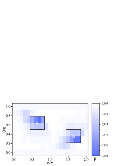
(a)

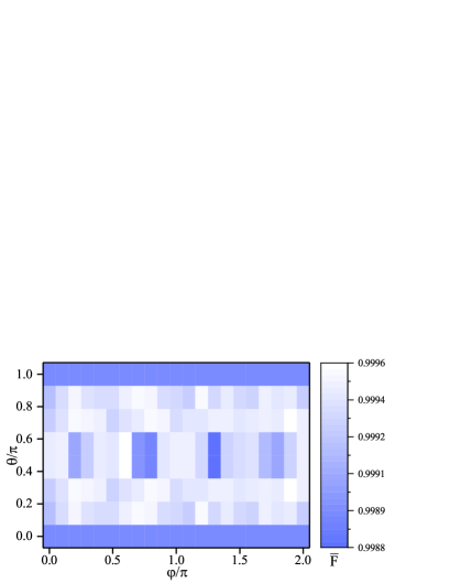
(b)

Figure 2: Average fidelities $\overline{F}$ distribution of preparing arbitrary single-qubit target state $\Psi(\theta,\varphi)$ using RG algorithm over 127 sampled tasks. (a) The mean of all average fidelities $\langle\overline{F}\rangle=0.973$ in DQDs system with $T=2\pi$ and $\mathrm{d}t=\pi/5$. The areas A and B are clustered bad points whose mean of average fidelities $\langle\overline{F}\rangle$ are 0.902 and 0.886 respectively. (b) The mean of all average fidelities $\langle\overline{F}\rangle=0.999$ in superconducting circuits system with $T=\pi$ and $\mathrm{d}t=\pi/5$.

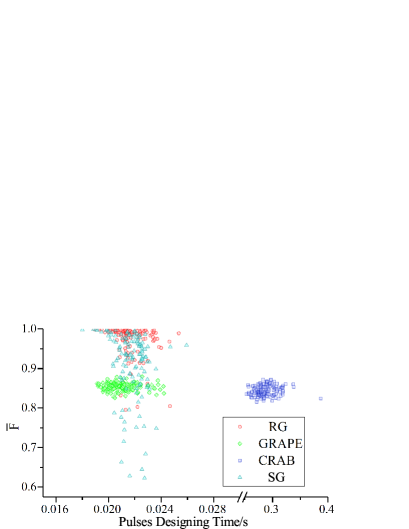
(a)

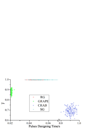
(b)

Figure 3: Average fidelities $\overline{F}$ versus designing time distributions of preparing arbitrary single-qubit target state over 127 sampled tasks with different optimization algorithms. The control parameters are identical to that adopted in Fig. 2. (a) State preparation in $S$-$T_{0}$ DQD, where the mean of all average fidelities $\langle\overline{F}\rangle=0.97273$, $0.85372$, $0.84407$, $0.91143$ and the mean of all average designing time $\langle\overline{t}\rangle=0.0217$, $0.0211$, $0.2877$, $0.0217$ with RG, GRAPE, CRAB and SG. (b) States preparation in Xmon superconducting circuits, where the mean of all average fidelities $\langle\overline{F}\rangle=0.99944$, $0.87807$, $0.69425$, $0.99937$ and the mean of all average designing time $\langle\overline{t}\rangle=0.0449$, $0.0214$, $0.9050$, $0.0520$ with RG, GRAPE, CRAB and SG.

The results of state preparation under different control parameters in two models are captured and shown in Table. 1. For visualization, Fig. 2 (a) and (b) plot the average preparation fidelity $\overline{F}$ of each single-qubit target state parameterized by angles $\theta$ and $\varphi$ in the context of semiconductor DQD and superconducting circuits respectively. The data correspond to the second and tenth rows of the Table. 1, respectively. In Fig. 2 (a), we can see that, although there’s only one degree of freedom, the fidelities of state preparation are high in most areas. Whereas there also some “bad points” exist and cluster together that cannot reach the target states well, e.g., the areas A and B, where the corresponding $\langle\overline{F}\rangle=0.902$ and $0.886,$ respectively. We ascribe this partially to the inappropriate parameter choice and believe it can be improved by further specifically tailoring parameters in these areas such as extended evolution time, altered action duration or more allowed actions. For example, leaving the other parameters intact, when $T=8\pi$, $\mathrm{d}t=\pi/3$, $\langle\overline{F}\rangle=0.992$ in both the A and B areas. In contrast, benefited from the additional degrees of freedom in $x$- and $y$-axes, the performance of state preparation in superconducting circuits is much better than in DQD, as shown in Fig. 2 (b), whose $\langle\overline{F}\rangle=0.999$ and the minimum $\overline{F}$ still exceeds $0.998$.

In addition, for comparing the performance of our scheme with the traditional optimization approaches, we plot the fidelities versus the corresponding runtime of designing pulses of our scheme plus the GRAPE, CRAB and SG for state preparation in DQDs and superconducting circuits in Fig. 3 (a) and (b) respectively, of which the control parameters are identical to that adopted in Fig. 2. To ensure a fair comparison, for GRAPE and CRAB, we discretize their continuous control strengths to the nearest allowed actions at the end of the execution to get the final solution. It can be seen that, our RG algorithm outperforms the GRAPE, CRAB, and SG with higher quality of state preparation in both $S$-$T_{0}$ DQD and Xmon superconducting single-qubit models. While, the runtime of designing proper control trajectory is in the same order of magnitude as the sophisticated GRAPE, which is known for high efficiency.

It is worth stating that, the reasons are different for the diversity of designing time in different algorithms: the runtime of GRAPE and CRAB are mainly brought about by the number of iterations; while the runtime of SG and RG are mainly caused by the minimum time steps to finish an episode. That is, the time steps in GRAPE and CRAB are fixed - $N=T/\mathrm{d}t$; yet the time steps in SG and RG are alterable, which may be smaller than $N$ only if the requirement to terminate the episode early is met. (See the details of the RG described in Sec. 2.) The RG favors a shorter path on the Bloch sphere between the initial and target states compared to other algorithms. Whereas, geometrically, this discrete control does not suffice to hit the quantum speed limit. We intend to make an another improved version of the SG utilizing pulses with continuous strength and duration to explore the speed limit of the similar quantum control problems in the future works.

3.2 Universal two-qubit state preparation with revised greedy algorithm

The control space for two-qubit state preparation in semiconductor DQDs is parameterized by the allowed pulse strengths in each qubit, i.e. $\{(J_{1},J_{2})|J_{1},J_{2}\in\{1,2,3,4,5\}\}$. Thus, there are $5\times 5=25$ allowed actions. As for two-qubit states preparation in superconducting circuits, the allowed actions on each qubit are same as these taken in the single-qubit case. The total number of allowed actions is $11\times 11=121$.

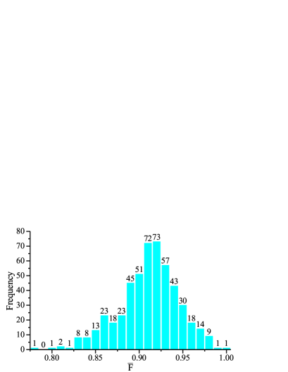
(a)

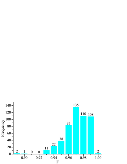
(b)

Figure 4: The frequency distributions of average fidelities $\overline{F}$ for two-qubit state preparation using RG algorithm over 511 sampled tasks. (a) The mean of all average fidelities $\langle\overline{F}\rangle=0.911$ in DQDs system with $T=10\pi$ and $\mathrm{d}t=\pi/2$. (b) The mean of all average fidelities $\langle\overline{F}\rangle=0.971$ in superconducting circuits system with $T=10\pi$ and $\mathrm{d}t=\pi/4$.

The detailed control parameters and the corresponding results in two models are listed in Table. 1. Meanwhile, Fig. 4 (a) and (b) plot the frequency distributions of average preparation fidelity $\overline{F}$ of each target point over sampled tasks in semiconductor DQDs and superconducting circuits, respectively. We can see that as an optimization method with low computational overhead, even in the case of lack of degrees of freedom, it still performs well in some certain points. It is worth pointing out that again each $\overline{F}$ of target point is over 511 preparation tasks, thus a high-valued $\overline{F}$ implies hundreds of successes of precise state preparation tasks. While these bad points can also perform better, in general, by carefully selecting parameters as it is in the case of single-qubit. For example, if the “worst point” in Fig. 4 (a) (whose $\overline{F}=0.779$, under $T=10\pi$ and $\mathrm{d}t=\pi/2$) is performed under $T=18\pi$ and $\mathrm{d}t=\pi/2$, its $\overline{F}$ can also reach 0.813.

Table 1: List of parameters and the corresponding average fidelity over all sampled state preparation tasks in four cases.

Model	Qubit	$T$	$\mathrm{d}t$	$\langle\overline{F}\rangle$
DQDs	Single-	$\pi$	$\pi/10$	0.951
		2$\pi$	$\pi/5$	0.973
		3$\pi$	$\pi/3$	0.977
		4$\pi$	$\pi/3$	0.983
	Two-	5$\pi$	$\pi/2$	0.894
		10$\pi$	$\pi/2$	0.911
		15$\pi$	$\pi/2$	0.930
		20$\pi$	$\pi/2$	0.938
Superconducting ciruits	Single-	$\pi$	$\pi/3$	0.983
		$\pi$	$\pi/5$	0.999
		$\pi$	$\pi/10$	0.998
		$\pi$	$\pi/20$	0.999
	Two-	5$\pi$	$\pi/4$	0.964
		10$\pi$	$\pi/4$	0.971
		12$\pi$	$\pi/4$	0.975
		15$\pi$	$\pi/4$	0.977

3.3 Universal state preparation in noisy environment

In the previous two subsections, we have explored the performance of our scheme in realizing the universal state preparation neglecting the effects of noises stemming from the surrounding environment and errors arising from systemic imperfections. Now we turn our attention to the robustness of this approach against various adverse factors.

There are many manifestations of imperfections, and we roughly categorize them into two classes: the static drifts and the dynamic fluctuations. Their impact on the evolution of the system can be taken into account by substituting the pertaining control parameter $f$ with the control-noise term $f+\delta$ or $f+\delta(t)$ in the corresponding Hamiltonian, respectively. The static drifts could be brought about by the misaligned control field or constant disturbance from the environment. While the dynamic fluctuations may originate from various time-dependent random control errors and stochastic noises from the environment, such as the no-zero bandwidth of the microwave drive and the charge noises arising from the uncontrolled impurities in the host material [47, 51, 52]. Regardless of their individual statics, these dynamic fluctuations will in concert behave as a noise with normal distribution for the central limit theorem [49]. At each time step the amplitude of the dynamic noise term $\delta(t)$ will be sampled from a zero-mean normal function $N(0,\sigma)$, where $\sigma$ represents the standard deviation and indicates the amplitude of the noise in a sense. For simplicity, the noise term will be kept constant within a time step. We stress here that the noise term is added to the Hamiltonian after the control pulse consequence has been designed to study the performance of our scheme in face of unpredictable noises. The robustness of our scheme is verified by evaluating the average fidelity $\langle\overline{F}\rangle$ over all of the sampled preparing tasks under different types and strengths of imperfections.

For the single-qubit state preparation, the average fidelity $\langle\overline{F}\rangle$ versus the amplitudes of various static drifts and dynamic noises are plotted in Fig. 5 (a) and (b), respectively. The impacts of time-dependent errors and noises applied to the QD’s exchange coupling $J$ and Zeeman energy gap $h$ are investigated individually. Yet their impacts on Xmon are discussed together for simplicity, i.e., the strengths of imperfections applied to Xmon’ control parameters are identified. From Fig. 5 (a) and (b), we can see that the average fidelity in the QD system is most affected by the static drift in $J$ and the dynamic fluctuation in $h$. While for the superconducting Xmon qubit, overall, the high average fidelity is well maintained even when the system is faced with comparable noises and errors as in the QD system.

For the two-qubit state preparation, we make the assumption that the static drifts on each qubit are identical i.e., $\delta_{1}=\delta_{2}$ where the subscript refers to the corresponding qubit; while the dynamic noises on two qubits are different, i.e., $\delta_{1}(t)\neq\delta_{2}(t)$ where each $\delta(t)$ is sampled from the same normal function $N(0,\sigma)$ individually. The average fidelity $\langle\overline{F}\rangle$ of two considered systems as a function of the magnitude of static and dynamic imperfections is showed in Fig. 5 (c) and (d) respectively. It is obvious that the impact of the static drifts to the systems is similar to the case of single-qubit. However, for the two-qubit QDs system, it is more affected by the dynamic fluctuation in $J$ compared to the single-qubit case.

From the above analysis, we can conclude that, overall, these control trajectories designed by our scheme exhibit a robustness against various errors and noises.

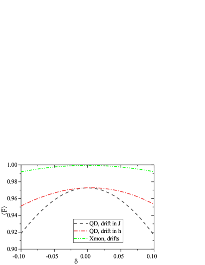
(a)

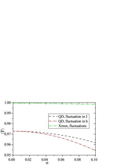
(b)

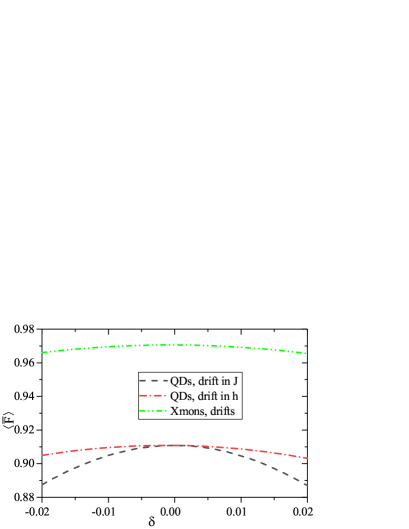
(c)

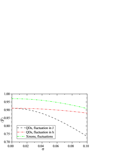
(d)

Figure 5: Average fidelites of the universal state preparation with RG algorithm over all preparing tasks versus amplitudes of different imperfections: (a) and (b) the static drifts and dynamic fluctuations in the parameters of single-qubit in semiconductor QD system and superconducting Xmon. (c) and (d) the static drifts and dynamic fluctuations in the parameters of two-qubit in semiconductor QDs system and superconducting Xmons.

Given the limitations of quantum computing hardware presently accessible, we simulate quantum computing on a classical computer and generate the corresponding data. Our algorithms are implemented with PYTHON 3.7.9 and QuTip 4.5.0, and have been run on a 64-core 3.40 GHz CPU with 125.6 GB memory. Details of the running environment of the algorithm can be found in the Sec. Data and code availability.

4 Conclusion

Precise and universal preparation of single- and two-qubit states is fundamental to quantum information and quantum computation. Yet the difficulty of designing control trajectory in complicated systems hinders the access to optimal solution for the driving between arbitrary quantum states. In this work, based on the standard greedy algorithm, we proposed a revised version, RG, to address this intractable problem. As demonstrations of our scheme, we apply it to the control of single- and two-qubit in the context of semiconductor DQDs and superconducting circuits and discovered a well performance, revealing its potential applicability. Compared with the typical numerical optimizations, our RG algorithm overcomes the local optimality and achieves a higher preparation quality. It is also demonstrated that the runtime of designing suited pulses with our scheme rivals to the GRAPE, which implies an outstanding efficiency. It outperforms the emerging machine learning approach with a well accessibility: could tailor the proper control trajectory to drive arbitrary initial state to other arbitrary target one without any training but only at a little cost of trial and error. We also discover that the control trajectories generated by our scheme are robust against various static and dynamic imperfections. As a radically different approach from previous methods, our scheme finds a new route to achieve quantum control optimization.

5 Models

Among the numerous promising qubit modalities, semiconductor quantum dots [53, 54, 55, 56, 57, 47, 58, 59, 60, 61] and superconducting circuits [62, 63, 64, 65, 49, 66, 67, 68, 69, 70, 71] have captured the imagination of the research field and become the leading candidates for their desirable merits, e.g. high scalability, long coherence time and desirable integration with well-established microfabrication. In this section, we introduce four models of single- and two-qubit in semiconductor DQDs and superconducting circuits.

5.1 Singlet-triplet qubits in semiconductor double quantum dots

There are many types of qubit have been proposed and demonstrated experimentally in semiconductor quantum dots, such as the spin or charge degrees of the electrons and donor nucleus [55, 57, 59, 61, 72, 60]. Due to the merit that it can be driven all electrically, the $S$-$T_{0}$ qubit in DQDs captures the most attention [73, 50, 74]. It is encoded by the spins of two electrons trapped in the potential created by charged electrodes on the surface of the heterostructure [55].

The effective Hamiltonian of a single $S$-$T_{0}$ qubit driven by external control field can be written as [47, 59, 75, 76, 72]

$$H(t)=J(t)\sigma_{z}+h\sigma_{x},$$ (3)

under the computational basis $\{|0\rangle,|1\rangle\}$, where $|0\rangle=|S\rangle=(|\uparrow\downarrow\rangle-|\downarrow\uparrow\rangle)/\sqrt{2}$ , $|1\rangle=|T_{0}\rangle=(|\uparrow\downarrow\rangle+|\downarrow\uparrow\rangle)/\sqrt{2}$. $h$ represents the Zeeman energy gap caused by local inhomogeneous micromagnetic field. Considering that for the micromagnetic field resulted by an integrated micromagnet, $h$ is hardly to vary during runtime, we therefore assume it as a constant and set $h=1$ here [50]. We also take the reduced Planck constant $\hbar=1$ throughout this work. The Pauli matrices $\sigma_{x}$, $\sigma_{y}$ and $\sigma_{z}$ indicate rotations about the $x$-, $y$- and $z$-axes of the Bloch sphere respectively. The exchange coupling $J(t)$ is the only tunable parameter in this model and can be modulated with electric pulses. In addition, it is physically restricted to be non-negative and bounded.

The properties of superposition of basis states and entanglement between multiple qubits are the source of the magic of quantum computing. In semiconductor DQDs, the interaction Hamiltonian of two entanglement qubits based on Coulomb interaction reads [74, 48, 73, 32]

$$H_{2\!-\!qubit}\!=\!\frac{\hbar}{2}\left(\begin{array}[]{cccc}J_{1}\!+\!J_{2}&h_{2}&h_{1}&0\\ h_{2}&J_{1}\!-\!J_{2}&0&h_{1}\\ h_{1}&0&J_{2}\!-\!J_{1}&h_{2}\\ 0&h_{1}&h_{2}&-J_{1}\!-\!J_{2}\!+\!2J_{12}\end{array}\right),$$ (4)

under the basis constituted by $\{|SS\rangle,|ST_{0}\rangle,|T_{0}S\rangle,|T_{0}T_{0}\rangle\}.$ $h_{i}$ and $J_{i}$ are the Zeeman energy gap and exchange interaction with the subscript $i=1,2$ referring to the corresponding qubit. The coupling strength between two qubits $J_{12}\propto J_{1}J_{2}$. To maintain the entanglement between two qubits, it has to keep $J_{i}>0$. We set $h_{1}=h_{2}=1$ and $J_{12}=J_{1}J_{2}/2$ here for simplicity.

5.2 Superconducting quantum circuits qubits

As a kind of “artificial atom”, the Hamiltonian of superconducting qubits can be designed just by tailoring the capacitance, inductance and Josephson energy [65]. According to the degrees of freedom and the ratio of Josephson energy to charging energy, superconducting qubits can mainly be classified into three categories: charge qubits [62], flux qubits [77] and phase qubits [78, 79]. Based on the above three archetypes, a variety of new types of superconducting qubits emerges, such as Transmon [80], Xmon [41, 42, 81], Gmon [82] and so on. Considering the representativeness of the Xmon type superconducting qubits, we take it as an example here. Nonetheless, this control scheme is also applicable to other superconducting qubit models.

When the qubit resonates with the microwave drive, the Hamiltonian of a single Xmon qubit in the rotating frame can be written as [49, 41, 42, 83]

$$H=\frac{\hbar}{2}A(\mathrm{cos}\phi\sigma_{x}+\mathrm{sin}\phi\sigma_{y}),$$ (5)

where $A$ and $\phi$ are the amplitude and phase of the microwave, respectively. Obviously, when $\phi=0$, $H=\frac{\hbar}{2}A_{x}\sigma_{x}$; in contrast, when $\phi=\pi/2$, $H=\frac{\hbar}{2}A_{y}\sigma_{y}$. Thus, the rotations about the $x$- and $y$-axes of the Bloch sphere can be obtained by properly setting $A$, $\phi$ and the duration $\tau$ of the microwave. In addition, the operation about the $z$-axis can be implemented physically by adjusting the current flowed into the superconducting quantum interference device loop through the so-called $Z$-line and the Hamiltonian can be expressed as [49, 83]

$$H=-\frac{\hbar}{2}A_{z}\sigma_{z},$$ (6)

when the $XY$ microwave drive is absent. $A_{z}$ is determined by the structure of the qubit as well as the current intensity and is bounded to be nonnegative and finite.

For two capacitively coupled Xmon qubits with same frequency, using rotating-wave approximation, the additional interaction term can be written as [65, 49, 83]

$$H_{couple}=\hbar g(\sigma_{1}^{+}\sigma_{2}^{-}+\sigma_{1}^{-}\sigma_{2}^{+}),$$ (7)

where $\sigma_{j}^{\pm}=\frac{1}{2}(\sigma_{x}^{j}\pm i\sigma_{y}^{j})$ with the superscript $j\in\{1,2\}$ referring to the corresponding qubit. $g$ is the coupling strength and we set $g=1$ here.

Data and code availability

The code, running environment of algorithm and all data used or presented in this paper are available from the corresponding author upon reasonable request or from Gitee in (https://gitee.com/herunhong/USP-via-RG).

References

References

- [1] Michael A Nielsen and Isaac L Chuang. Quantum computation and quantum information. 2015.
- [2] Bhupesh Bishnoi. Quantum-computation and applications, 06 2020.
- [3] P. Shor. Algorithms for quantum computation: discrete logarithms and factoring. In Proceedings of 35th Annual Symposium on the Foundations of Computer Science, IEEE Computer Society Press, Los Alamitos, CA, pages 124–134, 1994.
- [4] Richard P. Feynman. Simulating Physics with Computers, page 133–153. Perseus Books, USA, 1999.
- [5] I. M Georgescu, S Ashhab, and Franco Nori. Quantum simulation. Physics, 86(1):153–185, 2014.
- [6] L. K. Grover. A fast quantum mechanical algorithm for database search. Phys. Rev. Lett, 79, 1997.
- [7] Edward Farhi, Jeffrey Goldstone, and Sam Gutmann. A quantum approximate optimization algorithm. Eprint Arxiv, 2014.
- [8] S. Wang, Z. Wang, W. Li, L. Fan, G. Cui, Z. Wei, and Y. Gu. A quantum poisson solver implementable on nisq devices. arXiv:2005.00256v2, 2020.
- [9] Lieven MK Vandersypen and Isaac L Chuang. Nmr techniques for quantum control and computation. Reviews of modern physics, 76(4):1037, 2005.
- [10] Matthieud Bellec, Georgios M Nikolopoulos, and Stelios Tzortzakis. Faithful communication hamiltonian in photonic lattices. Optics letters, 37(21):4504–4506, 2012.
- [11] Armando Perez-Leija, Robert Keil, Hector Moya-Cessa, Alexander Szameit, and Demetrios N Christodoulides. Perfect transfer of path-entangled photons in j x photonic lattices. Physical Review A, 87(2):022303, 2013.
- [12] Philip Richerme, Zhe-Xuan Gong, Aaron Lee, Crystal Senko, Jacob Smith, Michael Foss-Feig, Spyridon Michalakis, Alexey V Gorshkov, and Christopher Monroe. Non-local propagation of correlations in quantum systems with long-range interactions. Nature, 511(7508):198–201, 2014.
- [13] J Casanova, A Mezzacapo, Jarrod Ryan McClean, L Lamata, Alan Aspuru-Guzik, E Solano, et al. From transistor to trapped-ion computers for quantum chemistry. Scientific Reports, 2014.
- [14] Lilian Childress and Ronald Hanson. Diamond nv centers for quantum computing and quantum networks. MRS bulletin, 38(2):134–138, 2013.
- [15] Romana Schirhagl, Kevin Chang, Michael Loretz, and Christian L. Degen. Nitrogen-vacancy centers in diamond: Nanoscale sensors for physics and biology. Annual Review of Physical Chemistry, 65(1):83, 2014.
- [16] Han Ning Dai, Bing Yang, Andreas Reingruber, Hui Sun, Xiao Fan Xu, Yu Ao Chen, Zhen Sheng Yuan, and Jian Wei Pan. Four-body ring-exchange interactions and anyonic statistics within a minimal toric-code hamiltonian. Nature Physics, 2017.
- [17] Mikko Mottonen, Juha J. Vartiainen, Ville Bergholm, and Martti M. Salomaa. Universal quantum computation. 2004.
- [18] Yumi Nakajima, Yasuhito Kawano, and Hiroshi Sekigawa. A new algorithm for producing quantum circuits using kak decompositions, 2006.
- [19] Colin P. Williams and Charles Bennett. Explorations in quantum computing. Physics Today, 52(2):66–68, 1999.
- [20] Farrokh, Vatan, Colin, and Williams. Optimal quantum circuits for general two-qubit gates. Physical Review A, 69(3):32315–32315, 2004.
- [21] Frederic T Chong, Franklin Diana, and Martonosi Margaret. Programming languages and compiler design for realistic quantum hardware. Nature, 549:180–187, 2018.
- [22] Alexandru Paler, Ilia Polian, Kae Nemoto, and Simon J Devitt. Fault-tolerant, high-level quantum circuits: form, compilation and description. Quantum Science ‘I&’ Technology, 2(2), 2015.
- [23] Xin Wang, Lev S Bishop, Edwin Barnes, JP Kestner, and S Das Sarma. Robust quantum gates for singlet-triplet spin qubits using composite pulses. Physical Review A, 89(2):022310, 2014.
- [24] Xin Wang, Lev S. Bishop, J. P. Kestner, Edwin Barnes, Kai Sun, and S. Das Sarma. Composite pulses for robust universal control of singlet-triplet qubits. Nature Communications, 3:997, 2013.
- [25] Robert E Throckmorton, Chengxian Zhang, Xu-Chen Yang, Xin Wang, Edwin Barnes, and S Das Sarma. Fast pulse sequences for dynamically corrected gates in singlet-triplet qubits. Physical Review B, 96(19):195424, 2017.
- [26] Xu-Chen Yang, Man-Hong Yung, and Xin Wang. Neural-network-designed pulse sequences for robust control of singlet-triplet qubits. Physical Review A, 97(4):042324, 2018.
- [27] Xiao Ming Zhang, Zezhu Wei, Raza Asad, Xu Chen Yang, and Xin Wang. When reinforcement learning stands out in quantum control? a comparative study on state preparation. Npj Quantum Information, 2019.
- [28] A. Zheng and D L Zhou. Deep reinforcement learning for quantum gate control. EPL (Europhysics Letters), 126(6):60002, 2019.
- [29] M. Y. Niu, S. Boixo, V. Smelyanskiy, and H. Neven. Universal quantum control through deep reinforcement learning. npj Quantum Information, 5(33), 2019.
- [30] Jian Lin, Zhong Yuan Lai, and Xiaopeng Li. Quantum adiabatic algorithm design using reinforcement learning. Phys. Rev. A, 101:052327, May 2020.
- [31] Z. T. Wang, Y. Ashida, and M. Ueda. Deep reinforcement learning control of quantum cartpoles. Physical Review Letters, 125(10), 2020.
- [32] Run Hong He, Rui Wang, Jing Wu, Shen Shuang Nie, Jia Hui Zhang, and Zhao Ming Wang. Deep reinforcement learning for universal quantum state preparation via dynamic pulse control. 2020.
- [33] Tobias Haug, Wai Keong Mok, Jia Bin You, Wenzu Zhang, Ching Eng Png, and Leong Chuan Kwek. Classifying global state preparation via deep reinforcement learning. Machine Learning: Science and Technology, 2(1):01LT02 (12pp), 2021.
- [34] C. Ferrie. Self-guided quantum tomography. Physical Review Letters, 113(19), 2014.
- [35] Navin Khaneja A, Timo Reiss B, Cindie Kehlet B, Thomas Schulte-Herbrüggen b, and Steffen J. Glaser B. Optimal control of coupled spin dynamics: design of nmr pulse sequences by gradient ascent algorithms - sciencedirect. Journal of Magnetic Resonance, 172(2):296–305, 2005.
- [36] B. Rowland and J. A. Jones. Implementing quantum logic gates with gradient ascent pulse engineering: principles and practicalities. Philos Trans A Math Phys Eng, 370(1976):4636–4650, 2012.
- [37] P. Doria, T. Calarco, and S. Montangero. Optimal control technique for many body quantum systems dynamics. Physical Review Letters, 106(19):237–251, 2010.
- [38] T. Caneva, T. Calarco, and S. Montangero. Chopped random-basis quantum optimization. Physical Review A, 84(2):17864–17875, 2011.
- [39] T Cormen, C Leiserson, and R Rivest. Introduction to algorithms, second edition. 2012.
- [40] Şebnem Yılmaz Balaman. Decision-Making for Biomass-Based Production Chains. 2019.
- [41] R. Barends, J. Kelly, A. Megrant, D. Sank, E. Jeffrey, Y. Chen, Y. Yin, B. Chiaro, J. Mutus, and C. Neill. Coherent josephson qubit suitable for scalable quantum integrated circuits. Physical Review Letters, 111(8):32–36, 2013.
- [42] P. J. J. O’Malley, R. Babbush, I. D. Kivlichan, J. Romero, J. R. McClean, R. Barends, J. Kelly, P. Roushan, A. Tranter, N. Ding, B. Campbell, Y. Chen, Z. Chen, B. Chiaro, A. Dunsworth, A. G. Fowler, E. Jeffrey, E. Lucero, A. Megrant, J. Y. Mutus, M. Neeley, C. Neill, C. Quintana, D. Sank, A. Vainsencher, J. Wenner, T. C. White, P. V. Coveney, P. J. Love, H. Neven, A. Aspuru-Guzik, and J. M. Martinis. Scalable quantum simulation of molecular energies. Phys. Rev. X, 6:031007, Jul 2016.
- [43] Richard S Sutton and Andrew G Barto. Reinforcement learning: An introduction. MIT press, 2018.
- [44] Ehsan, Zahedinejad, Joydip, Ghosh, Barry, C., and Sanders. High-fidelity single-shot toffoli gate via quantum control. Physical Review Letters, 114(20):200502–200502, 2015.
- [45] D J Egger and F K Wilhelm. Optimized controlled-z gates for two superconducting qubits coupled through a resonator. Superconductor Science and Technology, 27(1):014001, nov 2013.
- [46] Gian Giacomo Guerreschi and Jongsoo Park. Two-step approach to scheduling quantum circuits. Quantum Science and Technology, 3(4):045003, Jul 2018.
- [47] J. R Petta. Coherent manipulation of coupled electron spins in semiconductor quantum dots. Science, 309(5744):2180–2184, 2005.
- [48] Michael D Shulman, Oliver E Dial, Shannon P Harvey, Hendrik Bluhm, Vladimir Umansky, and Amir Yacoby. Demonstration of entanglement of electrostatically coupled singlet-triplet qubits. Science, 336(6078):202–205, 2012.
- [49] Philip Krantz, Morten Kjaergaard, Fei Yan, Terry P. Orlando, Simon Gustavsson, and William D. Oliver. A quantum engineer’s guide to superconducting qubits, 2019.
- [50] Xian Wu, Daniel R Ward, JR Prance, Dohun Kim, John King Gamble, RT Mohr, Zhan Shi, DE Savage, MG Lagally, Mark Friesen, et al. Two-axis control of a singlet–triplet qubit with an integrated micromagnet. Proceedings of the National Academy of Sciences, 111(33):11938–11942, 2014.
- [51] E. Barnes, Lukasz Cywinski, and S. D. Sarma. Nonperturbative master equation solution of central spin dephasing dynamics. Physical Review Letters, 109(14):140403–140403, 2012.
- [52] Ntt Nguyen and S. D. Sarma. Impurity effects on semiconductor quantum bits in coupled quantum dots. Physical review, 83(23):p.235322.1–235322.23, 2011.
- [53] Wonjin Jang, Min-Kyun Cho, Jehyun Kim, Hwanchul Chung, Vladimir Umansky, and Dohun Kim. Three individual two-axis control of singlet-triplet qubits in a micromagnet integrated quantum dot array. arXiv preprint arXiv:2009.13182, 2020.
- [54] TF Watson, SGJ Philips, Erika Kawakami, DR Ward, Pasquale Scarlino, Menno Veldhorst, DE Savage, MG Lagally, Mark Friesen, SN Coppersmith, et al. A programmable two-qubit quantum processor in silicon. Nature, 555(7698):633–637, 2018.
- [55] David M Zajac, Anthony J Sigillito, Maximilian Russ, Felix Borjans, Jacob M Taylor, Guido Burkard, and Jason R Petta. Resonantly driven cnot gate for electron spins. Science, 359(6374):439–442, 2018.
- [56] W Huang, CH Yang, KW Chan, T Tanttu, B Hensen, RCC Leon, MA Fogarty, JCC Hwang, FE Hudson, Kohei M Itoh, et al. Fidelity benchmarks for two-qubit gates in silicon. Nature, 569(7757):532–536, 2019.
- [57] Daniel Loss and David P. Divincenzo. Quantum computation with quantum dots. Physical Review A, 57(1):120–126, 1997.
- [58] Hendrik Bluhm, Sandra Foletti, Izhar Neder, Mark Rudner, and Amir Yacoby. Dephasing time of gaas electron-spin qubits coupled to a nuclear bath exceeding 200[thinsp][mu]s. Nature Physics, 7(2):109–113, 2010.
- [59] B. M. Maune, M. G. Borselli, B. Huang, T. D. Ladd, P. W. Deelman, K. S. Holabird, A. A. Kiselev, I. Alvarado-Rodriguez, R. S. Ross, and A. E. Schmitz. Coherent singlet-triplet oscillations in a silicon-based double quantum dot. Nature.
- [60] Xin Zhang, Hai Ou Li, Gang Cao, Ming Xiao, Guang Can Guo, and Guo Ping Guo. Semiconductor quantum computation. National Science Review, 6(01):38–60, 2019.
- [61] Xin Zhang, Hai Ou Li, Ke Wang, Gang Cao, Ming Xiao, and Guo Ping Guo. Qubits based on semiconductor quantum dots. Chinese Physics B, 27(02):20305–020305, 2018.
- [62] Nakamura, Y., Pashkin, Yu., A., Tsai, J., and S. Coherent control of macroscopic quantum states in a single-cooper-pair box. Nature, 398(6730):786–786, 1999.
- [63] Quantum supremacy using a programmable superconducting processor. Nature, 574(7779):505–510, 2019.
- [64] M. H. Devoret and R. J. Schoelkopf. Superconducting circuits for quantum information: An outlook. Science, 339(6124):1169–1174, 2013.
- [65] Wendin and Goran. Quantum information processing with superconducting circuits: a review. Reports on Progress in Physics, 2017.
- [66] Morten Kjaergaard, Mollie E. Schwartz, Jochen Braumüller, Philip Krantz, and William D. Oliver. Superconducting qubits: Current state of play. Annual Review of Condensed Matter Physics, 11(1), 2020.
- [67] Anton Frisk Kockum and Franco Nori. Quantum Bits with Josephson Junctions. 2019.
- [68] John Clarke and Frank K. Wilhelm. Superconducting quantum bits. Nature, 453(7198):1031–42, 2008.
- [69] Chao Song, Kai Xu, Wuxin Liu, Chuiping Yang, Shi Biao Zheng, Hui Deng, Qiwei Xie, Keqiang Huang, Qiujiang Guo, and Libo Zhang. 10-qubit entanglement and parallel logic operations with a superconducting circuit. Physical Review Letters, 2017.
- [70] Ming Gong, Shiyu Wang, Chen Zha, Ming-Cheng Chen, He-Liang Huang, Yulin Wu, Qingling Zhu, Youwei Zhao, Shaowei Li, Shaojun Guo, Haoran Qian, Yangsen Ye, Fusheng Chen, Chong Ying, Jiale Yu, Daojin Fan, Dachao Wu, Hong Su, Hui Deng, Hao Rong, Kaili Zhang, Sirui Cao, Jin Lin, Yu Xu, Lihua Sun, Cheng Guo, Na Li, Futian Liang, V. M. Bastidas, Kae Nemoto, W. J. Munro, Yong-Heng Huo, Chao-Yang Lu, Cheng-Zhi Peng, Xiaobo Zhu, and Jian-Wei Pan. Quantum walks on a programmable two-dimensional 62-qubit superconducting processor, 2021.
- [71] Yulin Wu, Wan-Su Bao, Sirui Cao, Fusheng Chen, Ming-Cheng Chen, Xiawei Chen, Tung-Hsun Chung, Hui Deng, Yajie Du, Daojin Fan, Ming Gong, Cheng Guo, Chu Guo, Shaojun Guo, Lianchen Han, Linyin Hong, He-Liang Huang, Yong-Heng Huo, Liping Li, Na Li, Shaowei Li, Yuan Li, Futian Liang, Chun Lin, Jin Lin, Haoran Qian, Dan Qiao, Hao Rong, Hong Su, Lihua Sun, Liangyuan Wang, Shiyu Wang, Dachao Wu, Yu Xu, Kai Yan, Weifeng Yang, Yang Yang, Yangsen Ye, Jianghan Yin, Chong Ying, Jiale Yu, Chen Zha, Cha Zhang, Haibin Zhang, Kaili Zhang, Yiming Zhang, Han Zhao, Youwei Zhao, Liang Zhou, Qingling Zhu, Chao-Yang Lu, Cheng-Zhi Peng, Xiaobo Zhu, and Jian-Wei Pan. Strong quantum computational advantage using a superconducting quantum processor, 2021.
- [72] Levy and Jeremy. Universal quantum computational with spin-1/2 pairs and heisenberg exchange. 89(14):1–3, 2002.
- [73] J. M. Taylor, H. A. Engel, W. Dur, A. Yacoby, C. M. Marcus, P. Zoller, and M. D. Lukin. Fault-tolerant architecture for quantum computation using electrically controlled semiconductor spins. NATURE PHYSICS, 2005.
- [74] John M Nichol, Lucas A Orona, Shannon P Harvey, Saeed Fallahi, Geoffrey C Gardner, Michael J Manfra, and Amir Yacoby. High-fidelity entangling gate for double-quantum-dot spin qubits. npj Quantum Information, 3(1):1–5, 2017.
- [75] Filip K Malinowski, Frederico Martins, Peter D Nissen, Edwin Barnes, Łukasz Cywiński, Mark S Rudner, Saeed Fallahi, Geoffrey C Gardner, Michael J Manfra, Charles M Marcus, et al. Notch filtering the nuclear environment of a spin qubit. Nature nanotechnology, 12(1):16, 2017.
- [76] Hendrik Bluhm, Sandra Foletti, Diana Mahalu, Vladimir Umansky, and Amir Yacoby. Universal quantum control of two electron spin qubits via dynamic nuclear polarization. APS, pages P17–008, 2009.
- [77] Mooij and E. J. Josephson persistent-current qubit. Science, 285(5430):1036, 1999.
- [78] John M. Martinis. Superconducting phase qubits. Quantum Information Processing, 8(2):81–103, 2009.
- [79] Matthew Neeley, Radoslaw C. Bialczak, M. Lenander, E. Lucero, Matteo Mariantoni, A. D. O’Connell, D. Sank, H. Wang, M. Weides, and J. Wenner. Generation of three-qubit entangled states using superconducting phase qubits. Nature.
- [80] Jens Koch, Terri M. Yu, Jay Gambetta, A. A. Houck, and R. J. Schoelkopf. Charge insensitive qubit design derived from the cooper pair box. Physics, 76(4):538–538, 2007.
- [81] J Kelly, R Barends, A. G Fowler, A Megrant, E Jeffrey, T. C White, D Sank, J. Y Mutus, B Campbell, and Yu Chen. State preservation by repetitive error detection in a superconducting quantum circuit. NATURE -LONDON-, 2015.
- [82] Qubit architecture with high coherence and fast tunable coupling. Physical Review Letters, 113(22):220502, 2014.
- [83] Heliang Huang, Dachao Wu, Daojin Fan, and Xiaobo Zhu. Superconducting quantum computing: A review. arXiv:2006.10433v3, 2020.