Unified formalism for electromagnetic and gravitational probes: densities

Abstract

The use of light front coordinates allows a fully relativistic description of a hadron’s spatial densities to be obtained. These densities must be two-dimensional and transverse to a chosen spatial direction. We explore their relationship to the three-dimensional, non-relativistic densities, with a focus on densities associated with the energy momentum tensor. The two-dimensional non-relativistic densities can be obtained from the light front densities through a non-relativistic limit, and can subsequently be transformed into three-dimensional non-relativistic densities through an inverse Abel transform. However, this operation is not invertible, and moreover the application of the inverse Abel transform to the light front densities does not produce a physically meaningful result. We additionally find that the Abel transforms of so-called Breit-frame densities generally differ significantly from the true light front densities. Numerical examples are provided to illustrate the various differences between the light front, Breit frame, and non-relativistic treatment of densities.

I Introduction

The energy momentum tensor (EMT) and the associated gravitational form factors Kobzarev and Okun (1962) have recently attracted significant interest in the hadron physics community. Major open questions such as the proton mass puzzle Ji (1995a, b); Lorcé (2018); Hatta et al. (2018) and proton spin puzzle Ashman et al. (1988); Ji (1997); Leader and Lorcé (2014) are directly related to the EMT. Moreover, the EMT encodes information about the magnitude and distribution of forces within hadrons Polyakov (2003); Polyakov and Schweitzer (2018); Lorcé et al. (2019); Freese and Miller (2021a), a topic which has itself led to a flurry of theoretical studies Polyakov and Schweitzer (2018); Lorcé et al. (2019), empirical extractions Burkert et al. (2018); Dutrieux et al. (2021); Burkert et al. (2021), and lattice calculations Shanahan and Detmold (2019).

The theoretical studies are driven by the promise of making relevant experiments to determine the various matrix elements that allow the extraction of the relevant form factors. As depicted in Fig. 1, the relevant formalism is most generally expressed through generalized transverse momentum distributions, which are obtained from bilocal correlation function $H_{\Gamma}(k,P,\Delta)$ by integrating over $k^{-}$. For quarks, this correlator is given by Diehl (2016):

$$H_{\Gamma}(k,P,\Delta)=\frac{1}{(2\pi)^{4}}\int\mathrm{d}^{4}z\,e^{ik\cdot z}\left\langle P+{1\over 2}\Delta\middle|\bar{q}\left(-{z\over 2}\right)\Gamma\mathcal{W}\left(-\frac{z}{2},\frac{z}{2}\right)q\left({z\over 2}\right)\middle|P-{1\over 2}\Delta\right\rangle\,,$$ (1)

where $\Gamma$ stands in for a matrix in the Dirac algebra (e.g., $\gamma^{+}$) and $\mathcal{W}(y,x)$ is a Wilson line from $x$ to $y$. Integration over $\mathbf{k}_{\perp}$ gives the generalized parton distribution, Mellin moments of which encode local form factors of interest—including those appearing in the EMT.

The form factors appearing in matrix elements of the EMT encode spatial densities via Fourier transforms. When performing these Fourier transforms, it is important to keep perspective about the actual, physical meaning of the densities that are obtained. It has been established Burkardt (2003); Miller (2007, 2009, 2019); Freese and Miller (2021a) that the only meaningful way to obtain fully relativistic densities is through two-dimensional Fourier transforms at fixed light front time. The three-dimensional Breit frame density is obtained by erroneously assuming that the hadron can be spatially localized Miller (2019); Jaffe (2021). Nonetheless, densities obtained through three-dimensional Fourier transforms unfortunately remain ubiquitous in the EMT density literature.

The Abel transform has recently been proposed as a means of connecting the light front and Breit frame formalisms Panteleeva and Polyakov (2021); Kim and Kim (2021). It is therefore necessary to explore the meaning of this connection. The Abel transform can be obtained by integrating one coordinate of a spherically symmetric density. However, there is no manifest spherical symmetry on the light front Brodsky et al. (1998). Additionally, Refs. Panteleeva and Polyakov (2021); Kim and Kim (2021) looked at the case of spin-half hadrons, but not spin-zero hadrons, where the proposed connection is shown below not to work.

The purpose here is to explore the actual meaning of 3D EMT densities and their relationship to the fully relativistic 2D light front densities. In particular, we show that physically meaningful 3D densities can be defined only in a non-relativistic approximation, either by taking $c\rightarrow\infty$ or—in some cases—keeping up to order $v^{2}/c^{2}$ corrections. Additionally, we examine the physical meaning and applicability of the Abel transform.

This work is organized as follows. In Sec. II, we discuss the Abel transform and when it does and does not connect 2D and 3D densities. In Sec. III, we consider the formalism for relativistic and non-relativistic densities for both spin-zero and spin-half particles, deriving results for the relationships between them. Numerical examples, based on using a simple hadronic model Miller (2009); Weinberg (1966); Gunion et al. (1973) are used to study the implications of using the Breit frame and the non-relativistic limit in Sec. IV. We conclude and provide a summary in Sec. V.

Figure 1: Chart depicting the relationships between densities in different formalisms, as well as their relationships to GPDs. Here, $\rho$ stands in for any space-dependent density, including mass density, $P^{+}$ density, or even pressure density. One-arrow (purple) lines signify one-way relationships, and two-arrow (green) lines signify invertible relationships. There is no systematic connection between light front and Breit frame densities.

II Abel transforms of physical densities

Since the fully relativistic light front densities are two-dimensional, they can be most directly compared to two-dimensional rather than three-dimensional non-relativistic densities. The 2D non-relativistic densities are obtained by integrating out one coordinate of a given three-dimensional density $\rho^{(3D)}_{\rm NR}({\bf r})$ (which may obtained as a three-dimensional Fourier transform of a form factor):

$$\rho_{\mathrm{NR}}^{(2D)}(\mathbf{b}_{\perp})=\int_{-\infty}^{\infty}\mathrm{d}z\,\rho_{\mathrm{NR}}^{(3D)}(\mathbf{r})\,,$$ (2)

where $\mathbf{b}_{\perp}=(x,y)$ are the transverse coordinates. If the 3D density is spherically symmetric, i.e., $\rho_{\mathrm{NR}}^{(3D)}(\mathbf{r})$ is a function of only $r=|\mathbf{r}|$, a change of integration variable allows us to write:

$$\rho_{\mathrm{NR}}^{(2D)}(b_{\perp})=2\int_{b}^{\infty}\mathrm{d}r\,\frac{r}{\sqrt{r^{2}-b_{\perp}^{2}}}\rho_{\mathrm{NR}}^{(3D)}(r)\equiv\mathscr{A}\Big{[}\rho_{\mathrm{NR}}^{(3D)}(r)\Big{]}(b_{\perp})\,,$$ (3)

which defines the Abel transform. For densities which depend on individual components of $\mathbf{r}$, one must use Eq. (2). However, each of the densities we consider can be written in terms of derivatives of an entirely scalar density to which Eq. (3) can be applied.

One pertinent property of the Abel transform is that it is invertible Bracewell (2000):

$$\rho_{\mathrm{NR}}^{(3D)}(r)=-\frac{1}{\pi}\int_{r}^{\infty}\mathrm{d}b_{\perp}\,\frac{\rho_{\mathrm{NR}}^{(2D)}(b_{\perp})}{\mathrm{d}b_{\perp}}\frac{1}{\sqrt{b_{\perp}^{2}-r^{2}}}\equiv\mathscr{A}^{-1}\Big{[}\rho_{\mathrm{NR}}^{(2D)}(b_{\perp})\Big{]}(r)\,.$$ (4)

This allows a 3D non-relativistic density to be reconstructed from a 2D non-relativistic density, assuming that we know the former to be spherically symmetric ahead of time.

The importance of spherical symmetry cannot be stressed enough. If one begins with an azimuthally symmetric 2D density without a guarantee of spherical symmetry in three dimensions, applying Eq. (4) may not give the correct 3D density. Consider, for instance, the following 3D densities:

$$f(r) =\frac{a^{3}}{(x^{2}+y^{2}+z^{2}+a^{2})^{3}}\,,$$ (5a)

$$g(\mathbf{r}) =\frac{sa^{3}}{(x^{2}+y^{2}+s^{2}z^{2}+a^{2})^{3}}\,,$$ (5b)

where $a$ is some length scale and $s$ is a positive unitless constant. These both integrate to the same azimuthally symmetric function:

$$\int_{-\infty}^{\infty}\mathrm{d}z\,f(r)=\int_{-\infty}^{\infty}\mathrm{d}z\,g(\mathbf{r})=\mathscr{A}\big{[}f(r)\big{]}(b)\equiv F(b)\,=\,{3a^{3}\pi\over 8(a^{2}+b^{2})^{5/2}}\,.$$ (6)

Applying the inverse Abel transform to $F(b)$ will return $f(r)$, even if—in the context of a physical scenario—$g(\mathbf{r})$ is the true 3D density.

This point is especially pertinent since the light front Galilean subgroup of the Poincaré group does not have an $\mathrm{SO}(3)$ subgroup. Light front dynamics does not admit 3D spherical symmetry Brodsky et al. (1998), so it is meaningless to try to construct an exact relativistic 3D density by applying Eq. (4) to a light front density, as done in Refs. Panteleeva and Polyakov (2021); Kim and Kim (2021) or earlier in Ref. Rajan et al. (2018). In fact, there are model calculations suggesting that the proton is elongated in the $x^{-}$ direction Miller and Brodsky (2020). Moreover, we shall see below that densities of transversely-polarized hadrons have $\phi$ dependence, demonstrating that spherical symmetry in $(\mathbf{x}_{\perp},x^{-})$ does not hold. At best, the inverse Abel transform of a light front density can give the 3D density in a non-relativistic approximation, as we shall show below.

One helpful property of Eq. (2) that will aid the exploration to follow is its effect on Fourier transforms. If a 3D density is defined by:

$$\rho_{\mathrm{NR}}^{(3D)}(r)=\int\frac{\mathrm{d}^{3}\bm{\Delta}}{(2\pi)^{3}}F(t=-\bm{\Delta}^{2})e^{-i\bm{\Delta}\cdot\mathbf{r}}\,,$$ (7)

then because the $z$ integral of $e^{-i\Delta_{z}z}$ is $2\pi\delta(\Delta_{z})$, one has:

$$\rho_{\mathrm{NR}}^{(2D)}(b_{\perp})=\int\frac{\mathrm{d}^{2}\bm{\Delta}_{\perp}}{(2\pi)^{2}}F(t=-\bm{\Delta}_{\perp}^{2})e^{-i\bm{\Delta}_{\perp}\cdot\mathbf{b}_{\perp}}\,.$$ (8)

III Relativistic and non-relativistic densities of the EMT

We shall now consider relativistic and non-relativistic densities of the energy momentum tensor (EMT). These densities are related to form factors, which are defined via matrix elements of plane wave states. For spin-zero particles, the standard decomposition is: is Polyakov and Schweitzer (2018):

$$\langle p^{\prime}|T^{\mu\nu}(0)|p\rangle=2P^{\mu}P^{\nu}A(t)+\frac{\Delta^{\mu}\Delta^{\nu}-\Delta^{2}g^{\mu\nu}}{2}D(t)\,,$$ (9)

while for spin-half particles Polyakov and Schweitzer (2018):

$$\langle p^{\prime},\lambda|T^{\mu\nu}(0)|p,\lambda\rangle=\bar{u}(p^{\prime},\lambda)\left\{\frac{P^{\mu}P^{\nu}}{M}A(t)+\frac{\Delta^{\mu}\Delta^{\nu}-\Delta^{2}g^{\mu\nu}}{4M}D(t)+\frac{iP^{\{\mu}\sigma^{\nu\}\rho}\Delta_{\rho}}{2M}J(t)\right\}u(p,\lambda)\,,$$ (10)

where $P=\frac{1}{2}\big{(}p+p^{\prime}\big{)}$, $\Delta=p^{\prime}-p$, $t=\Delta^{2}$, and curly brackets $\{\}$ signify symmetrization, e.g., $a^{\{\mu}b^{\nu\}}=a^{\mu}b^{\nu}+a^{\nu}b^{\mu}$.

III.1 Relativistic light front densities

As discussed in Refs. Brodsky et al. (1998); Burkardt (2003); Miller (2007), the only way to meaningfully define relativistic densities is at fixed light front time, since this allows separation between barycentric and relative coordinates. For both spin-zero hadrons and longitudinally polarized spin-half hadrons, the light front momentum ($P^{+}$) density is found to be Freese and Miller (2021a):

$$\rho_{P^{+}}^{(\mathrm{LF})}(\mathbf{b}_{\perp})=P^{+}\int\frac{\mathrm{d}^{2}\bm{\Delta}_{\perp}}{(2\pi)^{2}}A(t)e^{-i\bm{\Delta}_{\perp}\cdot\mathbf{b}_{\perp}}\,,$$ (11)

and in these same cases, the comoving stress tensor is Lorcé et al. (2019); Freese and Miller (2021a):

$$S_{\mathrm{LF}}^{ij}(\mathbf{b}_{\perp})=\frac{1}{4P^{+}}\Big{(}\delta^{ij}\bm{\nabla}_{\perp}^{2}-\bm{\nabla}_{\perp}^{i}\bm{\nabla}_{\perp}^{j}\Big{)}\int\frac{\mathrm{d}^{2}\bm{\Delta}_{\perp}}{(2\pi)^{2}}D(t)e^{-i\bm{\Delta}_{\perp}\cdot\mathbf{b}_{\perp}}\,.$$ (12)

This tensor can be decomposed into a isotropic pressure $p^{\mathrm{LF}(b_{\perp})}$ and pressure anisotropy (or shear stress function) $s^{\mathrm{LF}(b_{\perp})}(b_{\perp})$:

$$S_{\mathrm{LF}}^{ij}(\mathbf{b}_{\perp})=\delta^{ij}p^{(\mathrm{LF})}(b_{\perp})+\left(\frac{b_{\perp}^{i}b_{\perp}^{j}}{b_{\perp}^{2}}-\frac{1}{2}\delta^{ij}\right)s^{(\mathrm{LF})}(b_{\perp})\,,$$ (13)

and has eigenpressures in the tangential directions Lorcé et al. (2019); Panteleeva and Polyakov (2021); Freese and Miller (2021b):

$$p^{(\mathrm{LF})}_{r}(b_{\perp}) =\hat{b}_{i}\hat{b}_{j}S_{\mathrm{LF}}^{ij}(\mathbf{b}_{\perp})=p^{(\mathrm{LF})}(b_{\perp})+\frac{1}{2}s^{(\mathrm{LF})}(b_{\perp})$$ (14a)

$$p^{(\mathrm{LF})}_{t}(b_{\perp}) =\hat{\phi}_{i}\hat{\phi}_{j}S_{\mathrm{LF}}^{ij}(\mathbf{b}_{\perp})=p^{(\mathrm{LF})}(b_{\perp})-\frac{1}{2}s^{(\mathrm{LF})}(b_{\perp})\,.$$ (14b)

A useful quantity is the potential $\widetilde{D}(b_{\perp})$, defined by:

$$\widetilde{D}(b_{\perp}) =\frac{1}{4P^{+}}\int\frac{\mathrm{d}^{2}\bm{\Delta}_{\perp}}{(2\pi)^{2}}D(t)e^{-i\bm{\Delta}_{\perp}\cdot\mathbf{b}_{\perp}}\,.$$ (15)

The comoving stress tensor is related to this potential by:

$$S^{ij}(\mathbf{b}_{\perp}) =\Big{(}\nabla_{i}\nabla_{j}-\delta_{ij}\nabla^{2}\Big{)}\widetilde{D}(b_{\perp})\,.$$ (16)

The radial and tangential pressures have simple expressions in terms of the potential:

$$p_{r}(b_{\perp}) =\frac{1}{b_{\perp}}\frac{\mathrm{d}\widetilde{D}(b_{\perp})}{\mathrm{d}b_{\perp}}$$ (17a)

$$p_{t}(b_{\perp}) =\frac{\mathrm{d}^{2}\widetilde{D}(b_{\perp})}{\mathrm{d}b_{\perp}^{2}}\,.$$ (17b)

III.1.1 Transversely polarized hadrons

It’s possible to prepare spin-half hadrons in transversely polarized states, for which the light front densities will no longer have azimuthal symmetry. A transversely-polarized hadron can be prepared as a superposition of light front helicity states Carlson and Vanderhaeghen (2009):

$$|s_{T}=\mathbf{s}_{\perp}\rangle=\frac{\left|\lambda=+1\right\rangle+e^{i\phi_{s}}\left|\lambda=-1\right\rangle}{\sqrt{2}}\,.$$ (18)

In terms of helicity states, matrix elements of transversely polarized states take the form (with momentum dependence suppressed to compactify the formula):

$$\langle\mathbf{s}_{\perp}|\hat{O}|\mathbf{s}_{\perp}\rangle=\frac{1}{2}\Big{\{}\langle+|\hat{O}|+\rangle+\langle-|\hat{O}|-\rangle+\langle+|\hat{O}|-\rangle e^{i\phi_{s}}+\langle-|\hat{O}|+\rangle e^{-i\phi_{s}}\Big{\}}\,,$$ (19)

which is the average of helicity state densities, plus an additional $\phi$-dependent helicity-flip contribution.

The $P^{+}$ density of transversely polarized states is:

$$\rho_{P^{+},T}^{(\mathrm{LF})}(\mathbf{b}_{\perp},\mathbf{s}_{\perp})=\rho_{P^{+}}^{(\mathrm{LF})}(b_{\perp})+P^{+}\,\frac{\sin(\phi)}{2Mc}\frac{\mathrm{d}}{\mathrm{d}b_{\perp}}\int\frac{\mathrm{d}^{2}\bm{\Delta}_{\perp}}{(2\pi)^{2}}\Big{(}A(t)-2J(t)\Big{)}e^{-i\bm{\Delta}_{\perp}\cdot\mathbf{b}_{\perp}}\,,$$ (20)

where $\rho_{P^{+}}^{(\mathrm{LF})}(b_{\perp})$ is density for helicity states (equal to the spin-zero $P^{+}$ density in Eq. (11)), and $\phi=\phi_{b}-\phi_{s}$ is the angle from the transverse polarization vector to the transverse coordinate.

It’s worth remarking that the angular dependence is a strictly relativistic effect because taking the $c\rightarrow\infty$ limit eliminates the $\phi$ dependence.

The comoving stress tensor of also has angular dependence for transversely polarized states, and in addition has a new tensorial structure:

$$S^{ij}_{T}(\mathbf{b}_{\perp},\mathbf{s}_{\perp}) =\delta_{ij}p_{T}(b_{\perp},\phi)+\left(\hat{b}^{i}\hat{b}^{j}-\frac{1}{2}\delta^{ij}\right)s_{T}(b_{\perp},\phi)+\big{(}\hat{b}^{i}\hat{\phi}^{j}+\hat{b}^{j}\hat{\phi}^{i}\big{)}v_{T}(b_{\perp})$$ (21a)

$$p_{T}(b_{\perp},\phi) =p(b_{\perp})+\frac{\sin(\phi)}{2Mc}p^{\prime}(b_{\perp})$$ (21b)

$$s_{T}(b_{\perp},\phi) =s(b_{\perp})+\frac{\sin(\phi)}{2Mc}s^{\prime}(b_{\perp})$$ (21c)

$$v_{T}(b_{\perp},\phi) =\frac{\cos(\phi)}{2Mc}\frac{s(b_{\perp})}{b_{\perp}}\,,$$ (21d)

where $p(b_{\perp})$ and $s(b_{\perp})$ are the isotropic pressure and anisotropy functions in the helicity state case, and where $\hat{b}$ and $\hat{\phi}$ are unit vectors. The quantities $p_{T},\,s_{T},\,v_{T}$ cannot be obtained through an Abel transform.

The new tensor structure associated with $v_{T}(b_{\perp},\phi)$ is peculiar and does not contribute to either the radial or the tangential pressure, since it contracts with both $\hat{b}^{i}\hat{b}^{j}$ and with $\hat{\phi}^{i}\hat{\phi}^{j}$ to zero. It is more instructive—as discussed in Ref. Polyakov and Schweitzer (2018)—to find the eigenvalues and eigenvectors of the comoving stress tensor. Since the eigenvectors satisfy:

$$S^{ij}_{T}(\mathbf{b}_{\perp},\mathbf{s}_{\perp})\hat{e}_{\pm}^{j}=p_{\pm}(b_{\perp},\phi)\hat{e}_{\pm}^{i}\,,$$ (22)

where we use $\pm$ to index the two eigenvectors (and their associated eigenpressures), it is possible to write the pressure in any direction as a superposition of the eigenpressures. If we write the eigenvectors in terms of an angle with respect to the transverse spin vector:

$$\hat{e}_{\pm}=\cos(\theta_{\pm})\mathbf{s}_{\perp}+\sin(\theta_{\pm})\tilde{\mathbf{s}}_{\perp}\,,$$ (23)

then the eigenvectors of $S^{ij}_{T}(\mathbf{b}_{\perp},\mathbf{s}_{\perp})$ are given by the angles:

$$\theta_{+} =\phi+\frac{1}{2}\tan^{-1}\left(\frac{2v_{T}(b_{\perp},\phi)}{s_{T}(b_{\perp},\phi)}\right)$$ (24a)

$$\theta_{-} =\phi+\frac{1}{2}\tan^{-1}\left(\frac{2v_{T}(b_{\perp},\phi)}{s_{T}(b_{\perp},\phi)}\right)+\frac{\pi}{2}$$ (24b)

while the associated eigenpressures are given by:

$$p_{\pm}(b_{\perp},\phi) =p_{T}(b_{\perp},\phi)\pm\sqrt{\frac{1}{4}\big{(}s_{T}(b_{\perp},\phi)\big{)}^{2}+\big{(}v_{T}(b_{\perp},\phi)\big{)}^{2}}\,.$$ (24c)

In the limit of large $b_{\perp}$, one has $v_{T}(b_{\perp},\phi)\ll s_{T}(b_{\perp},\phi)$, so the eigen-angles become $\phi$ and $\phi+\frac{\pi}{2}$ very far from the center of the hadron. This deformation from the radial and tangential directions be seen as a relativistic effect that vanishes in the $c\rightarrow\infty$ limit, along with the angular dependence of the eigenpressures.

The angular dependence in both the $P^{+}$ density and the stress tensor demonstrates a lack of spherical symmetry in the light front formalism. This is of course not surprising, since rotations around the $x$ and $y$ axes are dynamical operators that do not commute with the light front Hamiltonian $P^{-}$ Dirac (1949); Brodsky et al. (1998). This finding precludes use of the inverse Abel transform to construct a physically meaningful 3D relativistic density. Moreover, the inverse Abel transform cannot even be applied at a formal level, since the transform acts on an azimuthally symmetric function of a single variable.

III.2 Breit frame densities

If one tries to define 3D relativistic densities at fixed instant form time, the density becomes contaminated by center-of-mass motion of the hadron as a whole Jaffe (2021). It is controversial whether localization of the center-of-mass motion in coordinate space is relativistically possible (see Refs. Newton and Wigner (1949); Kalnay and Toledo (1967); Pavšič (2018) for attempts, however), and localization in momentum space produces infinite radii for all densities Miller (2019) owing to the Heisenberg uncertainty principle.

Nonetheless, ostensibly relativistic 3D densities are ubiquitous throughout the hadron physics literature. The so-called Breit frame densities are defined by taking a Fourier transform of e.g. Eq. (9) with respect to the momentum transfer $\bm{\Delta}$ while setting the average momentum $\mathbf{P}=0$. It is worth stressing that these densities have not been derived from the basic definition of a physical density, i.e., expected value of a local current for a physical hadron state. As shown in Ref. Miller (2019), the original derivation in Ref. Sachs (1962) was erroneous and neglected a term that would make all radii infinite. Nonetheless, the erroneous Breit frame densities with finite radii are ubiquitous enough that they should be addressed, despite not being physically meaningful relativistic densities.

The Breit frame mass density and stress tensor both have different expressions for spin-zero and spin-half particles. For the mass density Polyakov (2003); Hudson and Schweitzer (2017); Polyakov and Schweitzer (2018):

$$\rho_{\mathrm{mass}}^{(j=0)}(\mathbf{r}) =M\int\frac{\mathrm{d}^{3}\bm{\Delta}}{(2\pi)^{3}}\frac{1}{\sqrt{1-\frac{t}{4M^{2}}}}\left\{A(t)-\frac{t}{4M}\Big{[}A(t)+D(t)\Big{]}\right\}e^{-i\bm{\Delta}\cdot\mathbf{r}}$$ (25a)

$$\rho_{\mathrm{mass}}^{(j=1/2)}(\mathbf{r}) =M\int\frac{\mathrm{d}^{3}\bm{\Delta}}{(2\pi)^{3}}\left\{A(t)-\frac{t}{4M}\Big{[}A(t)+D(t)-2J(t)\Big{]}\right\}e^{-i\bm{\Delta}\cdot\mathbf{r}}\,,$$ (25b)

while for the stress tensor:

$$T^{ij}_{\mathrm{BF},0}(\mathbf{r}) =\frac{1}{4M}\Big{(}\delta^{ij}\bm{\nabla}_{\perp}^{2}-\bm{\nabla}_{\perp}^{i}\bm{\nabla}_{\perp}^{j}\Big{)}\int\frac{\mathrm{d}^{3}\bm{\Delta}}{(2\pi)^{3}}\frac{1}{\sqrt{1-\frac{t}{4M^{2}}}}D(t)e^{-i\bm{\Delta}\cdot\mathbf{r}}$$ (26a)

$$T^{ij}_{\mathrm{BF},\frac{1}{2}}(\mathbf{r}) =\frac{1}{4M}\Big{(}\delta^{ij}\bm{\nabla}_{\perp}^{2}-\bm{\nabla}_{\perp}^{i}\bm{\nabla}_{\perp}^{j}\Big{)}\int\frac{\mathrm{d}^{3}\bm{\Delta}}{(2\pi)^{3}}D(t)e^{-i\bm{\Delta}\cdot\mathbf{r}}$$ (26b)

Using Eq. (8), it is possible to obtain simple formulas for the two-dimensional reductions of these Breit frame stress tensors. We find:

$$T^{ij}_{\mathrm{BF},0}(\mathbf{b}_{\perp}) =\frac{1}{4M}\Big{(}\delta^{ij}\bm{\nabla}_{\perp}^{2}-\bm{\nabla}_{\perp}^{i}\bm{\nabla}_{\perp}^{j}\Big{)}\int\frac{\mathrm{d}^{2}\bm{\Delta}_{\perp}}{(2\pi)^{2}}\frac{1}{\sqrt{1-\frac{t}{4M^{2}}}}D(t)e^{-i\bm{\Delta}_{\perp}\cdot\mathbf{b}_{\perp}}$$ (27a)

$$T^{ij}_{\mathrm{BF},\frac{1}{2}}(\mathbf{b}_{\perp}) =\frac{1}{4M}\Big{(}\delta^{ij}\bm{\nabla}_{\perp}^{2}-\bm{\nabla}_{\perp}^{i}\bm{\nabla}_{\perp}^{j}\Big{)}\int\frac{\mathrm{d}^{2}\bm{\Delta}_{\perp}}{(2\pi)^{2}}D(t)e^{-i\bm{\Delta}_{\perp}\cdot\mathbf{b}_{\perp}}\,,$$ (27b)

where the use of $\mathbf{b}_{\perp}$ instead of $\mathbf{r}$ is used to signify that these are 2D functions.

Comparing Eqs. (12,27b), one can see that $P^{+}S^{ij}_{\mathrm{LF}}(\mathbf{b}_{\perp})=MT^{ij}_{\mathrm{BF},\frac{1}{2}}(\mathbf{b}_{\perp})$, i.e., that the 2D Breit frame and light front comoving stress tensors have identical forms (up to a constant) for spin-half particles specifically. This is the essentially the central finding of Ref. Panteleeva and Polyakov (2021). The Abel transform connects 2D Breit frame densities to 3D Breit frame densities, and it just so happens that the Breit frame and light front comoving stress tensors have similar integrands specifically for spin-half particles. Because of this, Abel transforms formally work out to relate the 3D Breit frame and 2D light front pressures for spin-half particles. It should be recalled however that the light front does not have 3D spherical symmetry and that the Breit frame densities are not physically meaningful densities. Thus this formal coincidence does not have any deep physical meaning, and does not lend credence to the Breit frame pressure.

By contrast, one can easily observe that $P^{+}S^{ij}_{\mathrm{LF}}(\mathbf{b}_{\perp})\neq MT^{ij}_{\mathrm{BF},0}(\mathbf{b}_{\perp})$, so the findings of Ref. Panteleeva and Polyakov (2021) do not apply to spin-zero particles. 3D Breit frame pressures in spin-zero hadrons are not related to 2D light front pressures by Abel transforms. In light of the caveats we have stressed so far, this is not surprising, but it does help stress that the findings of Ref. Panteleeva and Polyakov (2021) originate from a coincidence rather than a deep connection between the light front and Breit frame.

III.3 Non-relativistic densities

In a non-relativistic (NR) quantum mechanical theory, just as in relativistic quantum field theory, the density associated with a local operator $\hat{\mathcal{O}}(x)$ and a physical state $|\Psi\rangle$ is given by:

$$\rho_{\mathrm{NR}}(\mathbf{r})=\langle\Psi|\hat{\mathcal{O}}(\mathbf{r})|\Psi\rangle_{\mathrm{NR}}\,.$$ (28)

The meaning of the term NR is that the system obeys Galilean invariance, in which the dependence on relative and center-of mass variables can be separated. The center of mass position of the physical state $|\Psi\rangle$ generally has a finite spatial extent. This state can be localized by allowing the total momentum to have infinite extent. This localization can be achieved, for example, by using a Gaussian representation Miller (2019) so that:

$$\Psi(\mathbf{p},\mathbf{s})=(2\pi)^{3/4}(2\sigma)^{3/2}e^{-\sigma^{2}\mathbf{p}^{2}}\,,$$ (29)

in which $\mathbf{p}$ refers to the total momentum of the system, and then taking the $\sigma\rightarrow 0$ limit at the end of the calculation. The spatial dependence of $\rho_{\mathrm{NR}}(\mathbf{r})$ thus defined will encode only internal structure of the hadron. It is possible to show (using similar derivations to those in Refs. Miller (2019); Freese and Miller (2021a)) that the density can be written:

$$\rho_{\mathrm{NR}}(\mathbf{r})=\lim_{\sigma\rightarrow 0}\,(2\pi)^{3/2}(2\sigma)^{3}\int\frac{\mathrm{d}^{3}\mathbf{P}}{(2\pi)^{3}}\int\frac{\mathrm{d}^{3}\bm{\Delta}}{(2\pi)^{3}}e^{-2\sigma^{2}\mathbf{P}^{2}}\langle\mathbf{p}^{\prime},\mathbf{s}|\hat{\mathcal{O}}(0)|\mathbf{p},\mathbf{s}\rangle_{\mathrm{NR}}e^{-\frac{\sigma^{2}}{2}\bm{\Delta}^{2}}e^{-i\bm{\Delta}\cdot\mathbf{r}}\,$$ (30)

in which $\mathbf{P}=\frac{1}{2}\big{(}\mathbf{p}+\mathbf{p}^{\prime}\big{)}$ and $\bm{\Delta}=\mathbf{p}^{\prime}-\mathbf{p}$. The limit $\sigma\rightarrow 0$ is to be taken after the $\mathbf{P}$ integral has been done. Integrals in which the matrix element contains factors $\mathbf{P}^{2}$, $\mathbf{P}^{4}$, etc. will diverge, which limits the densities that can be considered; for instance, we cannot calculate a kinetic energy density for a completely spatially localized system.

III.3.1 Non-relativistic reduction

The matrix element $\langle\mathbf{p}^{\prime},\mathbf{s}|\hat{\mathcal{O}}(0)|\mathbf{p},\mathbf{s}\rangle_{\mathrm{NR}}$ appearing in Eq. (30) is a non-relativistic matrix element. In practice, one knows how to express the relativistic counterpart $\langle\mathbf{p}^{\prime},\mathbf{s}|\hat{\mathcal{O}}(0)|\mathbf{p},\mathbf{s}\rangle_{\mathrm{rel}}$ in terms of local form factors. It should be possible to obtain the former from the latter by restoring factors of $c$ where appropriate and taking the $c\rightarrow\infty$ limit. Before doing so, we also must bear in mind that the momentum kets are normalized differently in the relativistic and non-relativistic cases; the conventional (instant form) normalization for momentum kets is:

$$\langle\mathbf{p}^{\prime},\mathbf{s}^{\prime}|\mathbf{p},\mathbf{s}\rangle_{\mathrm{NR}} =(2\pi)^{3}\delta^{(3)}(\mathbf{p}^{\prime}-\mathbf{p})\delta_{ss^{\prime}}$$ (31a)

$$\langle\mathbf{p}^{\prime},\mathbf{s}^{\prime}|\mathbf{p},\mathbf{s}\rangle_{\mathrm{rel}} =(2\pi)^{3}(2E_{\mathbf{p}})\delta^{(3)}(\mathbf{p}^{\prime}-\mathbf{p})\delta_{ss^{\prime}}\,.$$ (31b)

Thus, the fully non-relativistic (FNR) limit is given by:

$$\langle\mathbf{p}^{\prime},\mathbf{s}|\hat{\mathcal{O}}(0)|\mathbf{p},\mathbf{s}\rangle_{\mathrm{NR}}=\lim_{c\rightarrow\infty}\frac{1}{\sqrt{2E_{\mathbf{p}}2E_{\mathbf{p}^{\prime}}}}\langle\mathbf{p}^{\prime},\mathbf{s}|\hat{\mathcal{O}}(0)|\mathbf{p},\mathbf{s}\rangle_{\mathrm{rel}}\,.$$ (32)

Of course, one can take $E_{\mathbf{p}}/c^{2}\rightarrow M$ in the FNR limit, but in some cases it may be instructive to know what the leading relativistic corrections look like. These can be found by expanding the RHS of Eq. (32) as a power series in $|\mathbf{p}|/(Mc)$, and dropping terms beyond a certain order instead of taking the $c\rightarrow\infty$ limit.

When taking the non-relativistic limit, consistency demands that this limit be applied to the whole of the RHS of Eq. (32). For instance, in the case of the electric charge density of a spin-zero hadron, one has:

$$\langle\mathbf{p}^{\prime},\mathbf{s}|j^{0}(0)|\mathbf{p},\mathbf{s}\rangle_{\mathrm{NR}}=\lim_{c\rightarrow\infty}\left\{\frac{\big{(}E_{\mathbf{p}}+E_{\mathbf{p}^{\prime}}\big{)}}{\sqrt{2E_{\mathbf{p}}2E_{\mathbf{p}^{\prime}}}}F(t)\right\}=\lim_{c\rightarrow\infty}F(t)\equiv F_{\mathrm{NR}}(t)\,.$$ (33)

Since the dynamics that govern the structure of hadrons are manifestly relativistic, the form factor $F(t)$ will change in the non-relativistic limit, as seen for instance in Ref. Miller (2009). Consistent application of the non-relativistic limit thus means that the form factors appearing in non-relativistic 3D densities and fully relativistic light front densities should be different functions. We shall subscript the latter using NR.

III.3.2 Non-relativistic mass density

In the non-relativistic formalism, matrix elements of $T^{00}$ provide the mass density. For spin-zero and spin-half particles, respectively, we have:

$$\langle\mathbf{p}^{\prime},\mathbf{s}|T^{00}(0)|\mathbf{p},\mathbf{s}\rangle_{\mathrm{NR}}^{(j=0)}\approx Mc^{2}\Bigg{\{}\bigg{[}1 +\frac{\mathbf{P}^{2}}{2M^{2}c^{2}}+\frac{\bm{\Delta}^{2}}{8M^{2}c^{2}}\bigg{]}A_{\mathrm{NR}}(t)+\frac{\bm{\Delta}^{2}}{4M^{2}c^{2}}D_{\mathrm{NR}}(t)+\mathcal{O}(1/c^{4})\Bigg{\}}$$ (34a)

$$\langle\mathbf{p}^{\prime},\mathbf{s}|T^{00}(0)|\mathbf{p},\mathbf{s}\rangle_{\mathrm{NR}}^{(j=1/2)}\approx Mc^{2}\Bigg{\{}\bigg{[}1 +\frac{\mathbf{P^{2}}}{2M^{2}c^{2}}+\frac{\bm{\Delta}^{2}}{4M^{2}c^{2}}-\frac{i(\bm{\Delta}\times\mathbf{P})\cdot\mathbf{s}}{4M^{2}c^{2}}\bigg{]}A_{\mathrm{NR}}(t)$$

$$+\frac{\bm{\Delta}^{2}}{4M^{2}c^{2}}D_{\mathrm{NR}}(t)+\left[-\frac{\bm{\Delta}^{2}}{2M^{2}c^{2}}+\frac{i(\bm{\Delta}\times\mathbf{P})\cdot\mathbf{s}}{M^{2}c^{2}}\right]J_{\mathrm{NR}}(t)+\mathcal{O}(1/c^{4})\Bigg{\}}\,,$$ (34b)

where the NR subscripts on the form factors indicate that they should be expanded in powers of $1/c$ as well, and where here we use $|\mathbf{s}|=1$ for simplicity. Because of the $\mathbf{P}^{2}$ terms, these cannot be used to define densities for an arbitrarily localized hadron at order $1/c^{2}$, though the $c\rightarrow\infty$ limit does not have this issue. However, if this matrix element is placed into Eq. (30) without taking the $\sigma\rightarrow 0$ limit, one obtains results in the form:

$$\rho_{\mathrm{energy}}(\mathbf{r};\sigma)=\frac{\rho_{\mathrm{mass}}(\mathbf{r};\sigma)}{M}\left\{Mc^{2}+\frac{\langle\mathbf{P^{2}}\rangle_{\sigma}}{2M}\right\}+\mathcal{O}(1/c^{2})\,,$$ (35a)

where:

$$\langle\mathbf{P}^{2}\rangle_{\sigma} =\int\frac{\mathrm{d}^{3}\mathbf{P}}{(2\pi)^{3}}\,\mathbf{P}^{2}\,|\psi(\mathbf{P},\mathbf{s};\sigma)|^{2}=\frac{3}{\sigma^{2}}$$ (35b)

$$\rho_{\mathrm{mass}}^{(j=0)}(\mathbf{r};\sigma) =M\int\frac{\mathrm{d}^{3}\bm{\Delta}}{(2\pi)^{3}}\left\{A_{\mathrm{NR}}(t)+\frac{\bm{\Delta}^{2}}{8M^{2}c^{2}}\Big{[}A_{\mathrm{NR}}(t)+2D_{\mathrm{NR}}(t)\Big{]}\right\}e^{-i\bm{\Delta}\cdot\mathbf{r}}e^{-\frac{\sigma^{2}}{2}\bm{\Delta}^{2}}+\mathcal{O}(1/c^{4})$$ (35c)

$$\rho_{\mathrm{mass}}^{(j=1/2)}(\mathbf{r};\sigma) =M\int\frac{\mathrm{d}^{3}\bm{\Delta}}{(2\pi)^{3}}\left\{A_{\mathrm{NR}}(t)+\frac{\bm{\Delta}^{2}}{4Mc^{2}}\Big{[}A_{\mathrm{NR}}(t)+D_{\mathrm{NR}}(t)-2J_{\mathrm{NR}}(t)\Big{]}\right\}e^{-i\bm{\Delta}\cdot\mathbf{r}}e^{-\frac{\sigma^{2}}{2}\bm{\Delta}^{2}}+\mathcal{O}(1/c^{4})$$ (35d)

This has exactly the expected form of a mass density plus a (non-relativistic) kinetic energy density. Although we cannot take the $\sigma\rightarrow 0$ limit for the full (mass+kinetic) energy density at this order in $1/c^{2}$, we can actually take this limit for the mass density by itself. This suggests that we can obtain a meaningful leading-order relativistic correction to the mass density. This suggestion must however be tempered by the realization that the separation of energy into mass and kinetic energy requires the ability to bring the system to rest, which is explicitly precluded by taking the $\sigma\rightarrow 0$ limit.

It is worthwhile to observe that the NR+LO mass density for spin-half particles, as given in Eq. (35d) is identical in form to the Breit frame mass density given in Eq. (25b) (and previously found in Ref. Polyakov and Schweitzer (2018) for instance). A caveat worth mentioning is that consistency of the non-relativistic reduction requires expanding the form factors themselves in powers of $1/c$, while the Breit frame density uses the exact relativistic form factors. Moreover, such a coincidence does not occur for spin-zero particles.

The procedure outlined here cannot be used at arbitrarily high orders in $1/c$, and it is therefore not possible to define a fully relativistic 3D mass density through series of relativistic corrections. The dependence of $E_{\mathbf{p}}$ and $E_{\mathbf{p}^{\prime}}$ on $(\mathbf{P}\cdot\bm{\Delta})$ prevents factorizing the density integrand into a $\mathbf{P}$-dependent factor and $\bm{\Delta}$-dependent factor.

For both spin-zero and spin-half particles, the fully non-relativistic ($c\rightarrow\infty$) limit gives the same form for the mass density:

$$\rho_{\mathrm{mass}}^{(\mathrm{FNR})}(\mathbf{r}) =M\int\frac{\mathrm{d}^{3}\bm{\Delta}}{(2\pi)^{3}}A_{\mathrm{NR}}(t)e^{-i\bm{\Delta}\cdot\mathbf{r}}\,.$$ (36)

This is spherically symmetric, and comparison to Eqs. (8,11) shows that this is related to the non-relativistic limit of the fully relativistic $P^{+}$ density:

$$\rho_{\mathrm{mass}}^{(\mathrm{FNR})}(r)=\lim_{c\rightarrow\infty}\frac{M}{P^{+}}\mathscr{A}\Big{[}\rho_{P^{+}}^{(\mathrm{LF})}(b_{\perp})\Big{]}(r)\,.$$ (37)

We thus see that the inverse Abel transform of the $P^{+}$ density does have a physical meaning, if it is accompanied by the $c\rightarrow\infty$ limit: it gives the fully non-relativistic 3D mass density. Since the $c\rightarrow\infty$ limit is not invertible, this relation is not invertible either.

III.3.3 Non-relativistic stress tensor

The $T^{ij}$ components of the EMT give the stress tensor. It is worth stressing that $T^{ij}$ does not only encode pressure and shear forces, but also contains contributions from the motion of the system. For instance, taking the FNR limit for a spin zero system gives:

$$\langle\mathbf{p}^{\prime},\mathbf{s}|T^{ij}(0)|\mathbf{p},\mathbf{s}\rangle_{\mathrm{NR}}^{(j=0)} =\frac{\mathbf{P}^{i}\mathbf{P}^{j}}{M}A_{\mathrm{NR}}(t)+\left(\frac{\bm{\Delta}^{i}\bm{\Delta}^{j}-\delta_{ij}\bm{\Delta}^{2}}{4M}\right)D_{\mathrm{NR}}(t)+\mathcal{O}(1/c^{2})\,.$$ (38)

As it is, the stress tensor cannot be used with Eq. (30) unless the $\sigma\rightarrow 0$ limit is avoided, because the factor $\mathbf{P}^{i}\mathbf{P}^{j}$ multiplying $A(t)$ will produce a $\sigma^{-2}$ divergence when $i=j$. However, we can define a density at non-zero $\sigma$:

$$T^{ij}_{\mathrm{NR}}(\mathbf{r};\sigma)=\rho_{\mathrm{mass}}^{(\mathrm{NR})}(\mathbf{r};\sigma)\langle\mathbf{v}^{i}\mathbf{v}^{j}\rangle_{\sigma}+S^{ij}_{\mathrm{NR}}(\mathbf{r};\sigma)\,,$$ (39a)

in the FNR, where:

$$\langle\mathbf{v}^{i}\mathbf{v}^{j}\rangle_{\sigma} =\int\frac{\mathrm{d}^{3}\mathbf{P}}{(2\pi)^{3}}\,\frac{\mathbf{P}^{i}\mathbf{P}^{j}}{M^{2}}\,|\psi(\mathbf{P},\mathbf{s};\sigma)|^{2}=\frac{\delta_{ij}}{M^{2}\sigma^{2}}\,,$$ (39b)

$$S^{ij}_{\mathrm{NR}}(\mathbf{r};\sigma) =\int\frac{\mathrm{d}^{3}\bm{\Delta}}{(2\pi)^{3}}\left(\frac{\bm{\Delta}^{i}\bm{\Delta}^{j}-\delta_{ij}\bm{\Delta}^{2}}{4M}\right)D_{\mathrm{NR}}(t)e^{-i\bm{\Delta}\cdot\mathbf{r}}e^{-\frac{\sigma^{2}}{2}\bm{\Delta}^{2}}\,.$$ (39c)

This has the form expected of the classical non-relativistic stress tensor, with a piece encoding movement of the system and a piece expressing the comoving stress tensor $S^{ij}$. The comoving stress tensor is invariant under Galilean boosts, and thus can be interpreted as the stress tensor as seen by a comoving observer—a physical interpretation that is justified by having taken the fully non-relativistic limit.

The comoving stress tensor is well-defined in the $\sigma\rightarrow 0$ limit:

$$S^{ij}_{\mathrm{NR}}(\mathbf{r})=\frac{1}{4M}\Big{(}\delta^{ij}\bm{\nabla}^{2}-\bm{\nabla}^{i}\bm{\nabla}^{j}\Big{)}\int\frac{\mathrm{d}^{3}\bm{\Delta}}{(2\pi)^{3}}D_{\mathrm{NR}}(t)e^{-i\bm{\Delta}\cdot\mathbf{r}}\,.$$ (40)

It is straightforward to show that $S^{ij}_{\mathrm{NR}}(\mathbf{r})$ also has this form for spin-half systems.

The leading relativistic corrections introduce factors of $\mathbf{P}^{2}$ and $(\mathbf{P}\cdot\bm{\Delta})^{2}$ that preclude using the $\mathcal{O}(1/c^{2})$ corrections to define a density via Eq. (30). Moreover, outside of the fully non-relativistic limit, the isolation of a comoving stress tensor is not clear, and the latter is certainly no longer invariant under boosts. We thus constrain ourselves to considering the fully non-relativistic limit for the stress tensor.

As explained in Refs. Polyakov and Schweitzer (2018); Lorcé et al. (2019), this comoving stress tensor can be decomposed into an isotropic pressure $p(r)$ and a pressure anisotropy $s(r)$:

$$S_{\mathrm{NR}}^{ij}(\mathbf{r})=\delta^{ij}p^{(\mathrm{NR})}(r)+\left(\frac{r^{i}r^{j}}{r^{2}}-\frac{1}{3}\delta^{ij}\right)s^{(\mathrm{NR})}(r)\,.$$ (41)

By contracting this with unit vectors, it is possible to obtain directional pressures, e.g. radial and tangential pressures Polyakov and Schweitzer (2018); Lorcé et al. (2019):

$$p_{r}^{(\mathrm{NR})}(r) =\hat{r}_{i}\hat{r}_{j}S_{\mathrm{NR}}^{ij}(\mathbf{r})=p^{(\mathrm{NR})}(r)+\frac{2}{3}s^{(\mathrm{NR})}(r)$$ (42a)

$$p^{(\mathrm{NR})}_{t}(r) =\hat{\phi}_{i}\hat{\phi}_{j}S_{\mathrm{NR}}^{ij}(\mathbf{r})=p^{(\mathrm{NR})}(r)-\frac{1}{3}s^{(\mathrm{NR})}(r)\,.$$ (42b)

By integrating out the $z$ coordinate, one can obtain the 2D non-relativistic stress tensor:

$$S^{ij}_{\mathrm{NR}}(\mathbf{b}_{\perp})=\frac{1}{4M}\Big{(}\delta^{ij}\bm{\nabla}_{\perp}^{2}-\bm{\nabla}_{\perp}^{i}\bm{\nabla}_{\perp}^{j}\Big{)}\int\frac{\mathrm{d}^{2}\bm{\Delta}_{\perp}}{(2\pi)^{2}}D_{\mathrm{NR}}(t)e^{-i\bm{\Delta}_{\perp}\cdot\mathbf{b}_{\perp}}\,,$$ (43)

where dependence on $\mathbf{b}_{\perp}$ instead of $\mathbf{r}$ signifies that this is a 2D function. This can be compared to the light front comoving stress tensor in Eq. (12), giving:

$$S^{ij}_{\mathrm{NR}}(\mathbf{b}_{\perp})=\lim_{c\rightarrow\infty}\frac{P^{+}}{M}S^{ij}_{\mathrm{LF}}(\mathbf{b}_{\perp})\,.$$ (44)

By comparing the 3D non-relativistic eigenpressures in Eq. (42) to the 2D light front eigenpressures in Eq. (14), it is possible also to show that:

$$p_{t}^{(\mathrm{NR})}(r) =\lim_{c\rightarrow\infty}\frac{P^{+}}{M}\mathscr{A}^{-1}\big{[}p_{t}^{(\mathrm{LF})}(b_{\perp})\big{]}(r)$$ (45a)

$$p_{r}^{(\mathrm{NR})}(r) =\lim_{c\rightarrow\infty}\frac{2P^{+}}{M}\mathscr{A}^{-1}\big{[}p_{r}^{(\mathrm{LF})}(b_{\perp})\big{]}(r)\,.$$ (45b)

These are compatible with the spin-half results of Ref. Panteleeva and Polyakov (2021), although our result applies to spin-zero particles as well. Just as with the $P^{+}$ density, we find that the inverse Abel transform has a physical meaning when accompanied by the $c\rightarrow\infty$ limit: it produces the 3D densities in the fully non-relativistic limit.

III.3.4 Non-relativistic form factors

The connection between the 3D non-relativistic densities and the 2D light front densities, as given in Eqs. (37,45) are not invertible. This is so because the $c\rightarrow\infty$ limit cannot be undone. However, if the $c\rightarrow\infty$ limit had no effect on the form factors—i.e., if $A_{\mathrm{NR}}(t)=A(t)$ and $D_{\mathrm{NR}}(t)=D(t)$—then these relationships would actually be invertible. However, this is not the case, and we illustrate these points in the next section using a simple model.

IV Model calculations

We will now illustrate the findings of this work with pedagogical model calculations, specifically using a generalization Miller (2009) of the $\phi^{3}$ model first used by Weinberg Weinberg (1966) and later by by Gunion et al. Gunion et al. (1973). We use the interaction Lagrangian:

$$\mathscr{L}_{I}[\Psi,\phi,\xi]=g\Psi(x)\phi(x)\xi(x)\,,$$ (46)

where all of the three different fields are spin-zero bosons. The $\Psi$ particle of mass $M$ represents the bound state of the two different constituents $\phi$ and $\xi$, of masses $m_{1}$ and $m_{2}$ respectively.

The point-like coupling of this model is very simple, which is a pedagogic advantage, but short distance effects are emphasized Miller (2009) as the light-front wave function has a logarithmic divergence for small values of the transverse separation $b_{\perp}$ between the quarks. Furthermore, the asymptotic behavior of the electromagnetic form factor is $F(t)\sim{\log^{2}(-t)\over(-t)}$.

The electromagnetic current of the three-scalar model is given by:

$$\langle p^{\prime}|j^{\mu}(0)|p\rangle=2P^{\mu}F(t) =ig^{2}e_{1}\int\frac{\mathrm{d}^{4}k}{(2\pi)^{4}}\frac{2k^{\mu}}{\big{[}(k-P)^{2}-m_{2}^{2}\big{]}\big{[}(k+\Delta/2)^{2}-m_{1}^{2}\big{]}\big{[}(k-\Delta/2)^{2}-m_{1}^{2}\big{]}}$$

$$+ig^{2}e_{2}\int\frac{\mathrm{d}^{4}k}{(2\pi)^{4}}\frac{2k^{\mu}}{\big{[}(k-P)^{2}-m_{1}^{2}\big{]}\big{[}(k+\Delta/2)^{2}-m_{2}^{2}\big{]}\big{[}(k-\Delta/2)^{2}-m_{2}^{2}\big{]}}\,,$$ (47)

where $P=\frac{1}{2}\big{(}p+p^{\prime}\big{)}$ and $\Delta=p^{\prime}-p$. This is a sum of contributions from the constituents with masses $m_{1}$ and $m_{2}$. The $++$ component of the gravitational current is given by:

$$\langle p^{\prime}|T^{++}(0)|p\rangle=2(P^{+})^{2}A(t) =ig^{2}\int\frac{\mathrm{d}^{4}k}{(2\pi)^{4}}\frac{2(k^{+})^{2}}{\big{[}(k-P)^{2}-m_{2}^{2}\big{]}\big{[}(k+\Delta/2)^{2}-m_{1}^{2}\big{]}\big{[}(k-\Delta/2)^{2}-m_{1}^{2}\big{]}}$$

$$+ig^{2}\int\frac{\mathrm{d}^{4}k}{(2\pi)^{4}}\frac{2(k^{+})^{2}}{\big{[}(k-P)^{2}-m_{1}^{2}\big{]}\big{[}(k+\Delta/2)^{2}-m_{2}^{2}\big{]}\big{[}(k-\Delta/2)^{2}-m_{2}^{2}\big{]}}\,,$$ (48)

and to isolate $D(t)$ we look at the $12$ component:

$$\langle p^{\prime}|T^{12}(0)|p\rangle={1\over 2}\Delta^{1}\Delta^{2}D(t) =ig^{2}\int\frac{\mathrm{d}^{4}k}{(2\pi)^{4}}\frac{(k_{1}-\Delta_{1}/2)(k_{2}+\Delta_{2}/2)+(k_{2}-\Delta_{2}/2)(k_{1}+\Delta_{1}/2)}{\big{[}(k-P)^{2}-m_{2}^{2}\big{]}\big{[}(k+\Delta/2)^{2}-m_{1}^{2}\big{]}\big{[}(k-\Delta/2)^{2}-m_{1}^{2}\big{]}}$$

$$+ig^{2}\int\frac{\mathrm{d}^{4}k}{(2\pi)^{4}}\frac{(k_{1}-\Delta_{1}/2)(k_{2}+\Delta_{2}/2)+(k_{2}-\Delta_{2}/2)(k_{1}+\Delta_{1}/2)}{\big{[}(k-P)^{2}-m_{1}^{2}\big{]}\big{[}(k+\Delta/2)^{2}-m_{2}^{2}\big{]}\big{[}(k-\Delta/2)^{2}-m_{2}^{2}\big{]}}\,.$$ (49)

In particular, we shall consider examples with masses appropriate for a spin-less deuteron and a scalar pion. In that case, we take $m_{1}=m_{2}=m$. To simplify the notation, we additionally take $e_{1}+e_{2}=1$.

The integrals above can be evaluated using Feynman parameters. It is useful to start by considering the forward limit $\Delta^{\mu}=0$. Then:

$$F(0)={g^{2}\over 16\pi^{2}}\int_{0}^{1}\mathrm{d}x{(1-x)x\over{\cal M}^{2}(x)}\,,$$ (50)

with

$${\cal M}^{2}(x)\equiv m^{2}-x(1-x)M^{2}\,.$$ (51)

The coupling constant $g$ is chosen to yield $F(0)=1$. An important consistency check that

$$A(0)=F(0)$$ (52)

is satisfied. We also find that

$$D(0)=-{g^{2}\over 8\pi^{2}}\int_{0}^{1}\mathrm{d}x\,(1-x){1-(1-x)^{2}/3\over{\cal M}^{2}(x)}\,.$$ (53)

Defining the positive binding energy to be $B$ with $M=2m+B$ we find:

$$\lim_{B\to 0}D(0) =-{11\over 3}+{32\over 3\pi}\sqrt{B\over 2M}-{\cal O}\left({B\over M}\right)$$ (54a)

$$\lim_{B\to\infty}D(0) =-5+{2\over 15}\left({2M\over M+B}\right)^{2}+{\mathcal{O}}\left({M^{4}\over B^{4}}\right)\,.$$ (54b)

An equivalent procedure Miller (2009) to the use of Feynman parameters is to use the Drell-Yan frame, where $\Delta^{+}=0$, and integrate over $k^{-}\equiv k^{0}-k^{3}$. This enables one to obtain form factors in terms of light-front wave functions, and also simplifies taking the non-relativistic limit. We also use the relative momentum $\mbox{\boldmath$\kappa$}={\bf k}-x({\bf P}-\mbox{\boldmath$\Delta$}_{\perp}/2)$. The result is that:

$$F(t)={1\over 2(2\pi)^{3}}\int\mathrm{d}^{2}\mbox{\boldmath$\kappa$}\int_{0}^{1}{\mathrm{d}x\over x(1-x)}\psi^{*}(x,\mbox{\boldmath$\kappa$}+(1-x)\mbox{\boldmath$\Delta$}_{\perp})\psi(x,\mbox{\boldmath$\kappa$})\,,$$ (55)

as found in Ref. Gunion et al. (1973), with the frame-independent light-front wave function $\psi(x,\mbox{\boldmath$\kappa$})$ given by:

$$\psi(x,\mbox{\boldmath$\kappa$})\equiv g\left[M^{2}-{\mbox{\boldmath$\kappa$}^{2}+m_{1}^{2}\over x}-{\mbox{\boldmath$\kappa$}^{2}+m_{2}^{2}\over 1-x}\right]^{-1}\,,$$ (56)

where $\kappa$ is the $\perp$-component of the transverse relative momentum, and $x$ is the fractional component of the longitudinal plus-component of the momentum carried by the constituent of mass $m_{1}$.

For equal mass particles we find:

$$A(t)=F(t)$$ (57)

in this simple model, and identity that is very useful for deuteron-like kinematics, as we shall see below.

To aid in the calculations that follow, it is efficient to define a quantity:

$$G(\alpha,\mbox{\boldmath$\Delta$}) \equiv\int\mathrm{d}^{2}\mbox{\boldmath$\kappa$}\,\psi^{*}(x,\mbox{\boldmath$\kappa$}+\alpha\mbox{\boldmath$\Delta$}_{\perp})\psi(x,\mbox{\boldmath$\kappa$})\,,$$ (58)

with $\alpha$ as either $x$ or $1-x$, depending on which particle is probed. Then (for instance):

$$F(t)={1\over 16\pi^{3}}\int_{0}^{1}{\mathrm{d}x\over x(1-x)}G(1-x,\mbox{\boldmath$\Delta$}_{\perp})\,.$$ (59)

The use of Feynman parameters leads to the result:

$$G(\alpha,\mbox{\boldmath$\Delta$}) =2\pi g^{2}x^{2}{\bar{x}}^{2}\int_{0}^{1/2}\mathrm{d}z{1\over{\cal M}^{2}+\alpha^{2}Q^{2}(1/4-z^{2})}=4\pi g^{2}x^{2}{\bar{x}}^{2}\frac{\log\left(\frac{\sqrt{\alpha^{2}Q^{2}\left(4{\cal M}^{2}+\alpha^{2}Q^{2}\right)}+2{\cal M}^{2}-\alpha^{2}t}{2{\cal M}^{2}}\right)}{\sqrt{\alpha^{2}Q^{2}\left(4{\cal M}^{2}+\alpha^{2}Q^{2}\right)}}\,.$$ (60)

Transverse densities are 2D Fourier transforms of the relevant form factors, such as:

$$\rho_{F}(b_{\perp})=\int{\mathrm{d}^{2}\mbox{\boldmath$\Delta$}_{\perp}\over(2\pi)^{2}}e^{-i\mbox{\boldmath$\Delta$}_{\perp}\cdot{\bf b}_{\perp}}F(t)\,.$$ (61)

so that it is useful to introduce the coordinate-space wave function:

$$\psi(x,{\bf b}_{\perp})=\int{\mathrm{d}^{2}\kappa\over(2\pi)^{2}}\psi(x,\mbox{\boldmath$\kappa$})e^{i\mbox{\boldmath$\kappa$}\cdot{\bf b}_{\perp}}\,.$$ (62)

In this model:

$$\psi(x,b_{\perp})={1\over(2\pi)^{2}}\int\mathrm{d}^{2}\mbox{\boldmath$\kappa$}e^{i\mbox{\boldmath$\kappa$}\cdot{\bf b}}\psi(x,\kappa)={-g\over(2\pi)}x\bar{x}K_{0}({\cal M}b_{\perp})\,,$$ (63)

where $K_{0}(x)$ is a modified Bessel function of the second kind, and where $\bar{x}\equiv 1-x$. In terms of this wave function, the density corresponding to the electromagnetic form factor,, $\rho_{F}$ is given by:

$$\rho_{F}(b_{\perp})=\int_{0}^{1}{\mathrm{d}x\over(1-x)^{2}}\left|\psi\left(x,{b_{\perp}\over 1-x}\right)\right|^{2}\,.$$ (64)

Similarly, one may show that

$${1\over 2}\Delta_{1}\Delta_{2}D(t)=\int{\mathrm{d}^{2}\mbox{\boldmath$\kappa$}\over(2\pi)^{3}}\int_{0}^{1}{\mathrm{d}x\over x(1-x)}\Big{(}2\kappa_{1}\kappa_{2}-\Delta_{1}\Delta_{2}/2\Big{)}\left[{1\over x}\psi^{*}(x,\mbox{\boldmath$\kappa$}+(1-x)\mbox{\boldmath$\Delta$}_{\perp}/2)\,\psi(x,\mbox{\boldmath$\kappa$}-(1-x)\mbox{\boldmath$\Delta$}_{\perp}/2)\right]$$ (65)

Evaluation of the term proportional to $\kappa_{1}\kappa_{2}$ must result in a term proportional to $\Delta_{1}\Delta_{2}$. However, it is worthwhile to find an explicit expression for $D(t)$. This may be done by expressing $D(t)$ in terms of the coordinate-space wave function, $\psi(x,{\bf b}_{\perp})$. Some algebra leads to the expression:

$$D(t)=-4\int_{0}^{1}{\mathrm{d}x\over x(1-x)^{2}}\int\mathrm{d}b_{\perp}\,b_{\perp}|\psi^{\prime}(x,b_{\perp})|^{2}{J_{2}(x|\bm{\Delta}_{\perp}|b_{\perp})\over(-t)}-\int{\mathrm{d}x(1+x)\over x(1-x)}\int\mathrm{d}b_{\perp}\,b_{\perp}|\psi(x,b_{\perp})|^{2}J_{0}(x|\bm{\Delta}_{\perp}|b_{\perp})\,,$$ (66)

where: $\psi^{\prime}(x,b_{\perp})\equiv{\partial\psi(x,b)\over\partial b}\,.$ The quadrupole nature of $D(t)$ is exhibited by the appearance of the Bessel function of order 2 in Eq. (66).

The transverse density is obtained in the same way. For simplicity, we examine the light front version of Polyakov’s stress potential function $\widetilde{D}(b_{\perp})$ defined in Eq. (15). for which we find:

$$4P^{+}\,\widetilde{D}(b_{\perp})={-1\over\pi}\int{\mathrm{d}x\over x(1-x)}\left[f\left(x,\frac{b_{\perp}}{{\bar{x}}}\right)+{1\over 2}\bigg{(}{1-x^{2}\over x^{2}\bar{x}}\,\left|\psi\left(x,\frac{b_{\perp}}{x}\right)\right|^{2}\bigg{)}\right]\,,$$ (67a)

with

$$f(\alpha,b)\equiv\int_{b/\alpha}^{\infty}\mathrm{d}b^{\prime}_{\perp}\,b^{\prime}_{\perp}\left(1-{b^{2}\over\alpha^{2}{b^{\prime}}^{2}}\right)|\psi^{\prime}(\alpha,b^{\prime})|^{2}.$$ (67b)

The above derivation of $D(t)$ exhibits the dependence on the wave function and is thus useful in obtaining the non-relativistic limit. One may instead proceed more directly to determine $D(t)$ by starting with Eq. (65) and using Feynman parameters to obtain:

$$D(t)={-1\over 8\pi^{3}}\int_{0}^{1}\mathrm{d}x\,{1\over x^{2}\bar{x}}\widetilde{G}(\bar{x},t)$$ (68)

with

$$\widetilde{G}(\alpha,t)\equiv 2\pi g^{2}x^{2}{\bar{x}}^{2}\int_{0}^{1}\mathrm{d}y\,{(1-y^{2}\alpha^{2})\over{\cal M}^{2}-\alpha^{2}t/4(1-y^{2})}=8\pi g^{2}x^{2}{\bar{x}}^{2}\,\frac{|\bm{\Delta}_{\perp}|-\frac{\left(4-\left(\alpha^{2}-1\right)t\right)\tanh^{-1}\left(\frac{\alpha|\bm{\Delta}_{\perp}|}{\sqrt{4-\alpha^{2}t}}\right)}{\alpha\sqrt{4-\alpha^{2}t}}}{|\bm{\Delta}_{\perp}|^{3}}\,.$$ (69)

IV.1 Breit-frame densities and transverse pseudo-densities

The three dimensional Breit-frame densities are given in Sec. III.2 above. From these, one obtains the 2D Breit frame densities through an Abel transform. For spin-zero hadrons specifically, one has:

$$\widetilde{D}_{\mathrm{BF}}(b_{\perp})=\int_{-\infty}^{\infty}\mathrm{d}z\,\widetilde{D}_{\mathrm{BF}}(r)=\int{\mathrm{d}^{2}\bm{\Delta}_{\perp}\over(2\pi)^{2}}{D(t)\over\sqrt{1-t/(4M^{2})}}e^{-i\mbox{\boldmath$\Delta$}_{\perp}\cdot{\bf b}_{\perp}}\,,$$ (70)

for example. If $M\to\infty$ then $\widetilde{D}_{\mathrm{BF}}(b_{\perp})\rightarrow\widetilde{D}(b_{\perp})$, with the latter being the true (light front) relativistic density. Since the integral goes over all values of $t$, however, the equality does not hold. At best, one could have $\widetilde{D}_{\mathrm{BF}}(b_{\perp})\approx\widetilde{D}(b_{\perp})$ if $D(-t\to 4M^{2})\approx 0$. Therefore we refer to $\widetilde{D}_{\mathrm{BF}}(b_{\perp})$ as a transverse pseudo-density.

The integral appearing in Eq. (70) provides a numerical challenge because the asymptotic limit is $D(t)\sim\log^{2}(-t)/(-t)$. This means that an expansion in powers of $-t^{2}/4M^{2}$ diverges. A valid numerical procedure is obtained by relating $\widetilde{D}_{\mathrm{BF}}(b_{\perp})$ to the true transverse density $\widetilde{D}(b_{\perp})$. This is achieved by using Eq. (15) and the relation:

$$\int{\mathrm{d}^{2}\mbox{\boldmath$\Delta$}_{\perp}\over(2\pi^{2})}{e^{i\mbox{\boldmath$\Delta$}_{\perp}\cdot{\bf s}}\over\sqrt{1-t^{2}/(4M^{2})}}={1\over\pi}{e^{-2Ms}\over s}\,,$$ (71)

so that:

$$\widetilde{D}_{\mathrm{BF}}(b_{\perp})={M\over\pi}\int\mathrm{d}^{2}s\,\widetilde{D}\big{(}|{\bf b}_{\perp}-{\bf s}|\big{)}{e^{-2Ms}\over s}\,.$$ (72)

This expression is amenable to two-dimensional numerical integration.

IV.2 Non-relativistic limit

The conventional lore is that the electromagnetic form factor is the three-dimensional Fourier transform (3DFT) of the charge density. This idea emerges only by taking the fully non-relativistic limit.

We briefly review Miller (2009) how the 3DFT emerges. Our starting point is the wave function Eq. (56) and the form factor Eq. (55). Recall that the quantity $x=k^{+}/P^{+}$. In the non-relativistic limit the energy $k^{0}=m_{1}$, and $k^{+}=m_{1}+\kappa^{3}$, where $\kappa^{3}$ is the third-component of the relative longitudinal momentum. Further we define the positive binding energy $B$ so that

$$M\equiv m_{1}+m_{2}-B\,.$$ (73)

Then Brodsky and Lepage (1989); Frankfurt and Strikman (1981):

$$x=\frac{m_{1}+\kappa^{3}}{M},\quad 1-x=\frac{M-m_{1}-\kappa^{3}}{M}=\frac{m_{2}-B-\kappa^{3}}{M}\,.$$ (74)

To obtain the non-relativistic wave function we express the denominator appearing in Eq. (56) in terms of $\kappa^{3}$. This gives:

$$M^{2}-{\kappa^{2}+m_{1}^{2}\over x}-{\kappa^{2}+m_{2}^{2}\over 1-x}\approx 2M\left(-B-{\kappa^{2}\over 2\mu}\right)\,,$$ (75)

where:

$${\kappa}^{2}\equiv\mbox{\boldmath$\kappa$}^{2}+\kappa_{3}^{2}\,,\qquad\bm{\kappa}=\mbox{\boldmath$\kappa$}+\kappa^{3}\hat{{\bf z}}\,,\qquad\mu\equiv{m_{1}m_{2}\over m_{1}+m_{2}}\,.$$ (76)

In deriving Eq. (75), we have dropped terms of order $(v/c)^{3}=(k/m)^{3}$ and higher, and terms of order $B/M$ and higher. The result is that Eq. (75) is recognizable as $2M$ times the inverse of the non-relativistic propagator.

The next step is to determine the coordinate form of the non-relativistic wave function $\psi_{\mathrm{NR}}(\mathbf{r})$ (where $\mathbf{r}$ is canonically conjugate to $\bm{\kappa}$) and to show that the non-relativistic form factor is a three-dimensional Fourier transform of $\left|\psi_{\mathrm{NR}}(\mathbf{r})\right|^{2}$. First use the non-relativistic approximation Eq. (75) in Eq. (56) to find

$$\psi_{\mathrm{NR}}(\bm{\kappa})={-\mu g\over M(\kappa^{2}+\lambda^{2})}\,,\qquad\lambda^{2}\equiv 2\mu B.\,.$$ (77)

The coordinate-space wave function $\psi_{\mathrm{NR}}(\mathbf{r})$ is given by

$$\psi_{\mathrm{NR}}(\mathbf{r})={1\over(2\pi)^{3/2}}\int\mathrm{d}^{3}\bm{\kappa}\,e^{i\bm{\kappa}\cdot\mathbf{r}}\psi_{\mathrm{NR}}(\bm{\kappa})=-{\mu g\over 2M}\sqrt{\pi\over 2}{e^{-\lambda r}\over r}\,.$$ (78)

The expression Eq. (78) is seen as the standard result obtained for the bound state of a two-particle system interacting via an attractive delta function potential. It is also the effective range approximation Bethe and Longmire (1950), now known as the leading-order term in effective field theory Kaplan et al. (1999).

The wave functions Eq. (77) and Eq. (78) enable us to examine the conditions needed for the approximations Eq. (74) to be valid. For Eq. (74) to work, we need $\kappa^{2}\ll m_{1,2}^{2}$. The wave functions include all corrections to masses of order $\kappa^{2}/m_{1,2}^{2}$, and therefore no further corrections of order $\kappa/m_{1,2}$ or $B/m_{1,2}$ should be included. Thus in evaluating the form factor we should use

$$\mathrm{d}x \rightarrow{\mathrm{d}\bm{\kappa}^{3}\over M}$$ (79a)

$$x(1-x) \rightarrow{\mu\over M}$$ (79b)

$$(1-x)\mbox{\boldmath$\Delta$} \rightarrow{m_{2}\over M}\mbox{\boldmath$\Delta$}\,.$$ (79c)

The non-relativistic electromagnetic form factor $F_{\mathrm{NR}}(t)$ is obtained by using Eq. (77) in the expression for the form factor Eq. (55), and taking the non-relativistic limit as defined above. The result is

$$F_{\mathrm{NR}}(t)={1\over 2(2\pi)^{3}\mu}\int\mathrm{d}^{3}\mathbf{r}\,\left|\psi_{\mathrm{NR}}(\mathbf{r})\right|^{2}e^{-i\mbox{\boldmath$\Delta$}\cdot{\bf r}{m_{2}\over M}}\,.$$ (80)

This conforms to the commonplace expectation that the form factor is a three-dimensional Fourier transform of the density. One may extract the density $|\psi_{\mathrm{NR}}(b_{\perp})|^{2}$ by taking the Fourier transform of the form factor:

$$\int\mathrm{d}^{3}\bm{\Delta}\,F_{\mathrm{NR}}(t)e^{i\mbox{\boldmath$\Delta$}\cdot{\bf R}}={1\over 2\mu}\bigg{|}\psi_{\mathrm{NR}}\left({M\over m_{2}}R\right)\bigg{|}^{2}\,.$$ (81)

Similarly, the non-relativistic gravitational form factor is given by

$$A_{\mathrm{NR}}(t)={1\over 2(2\pi)^{3}\mu}\int\mathrm{d}^{3}\mathbf{r}\,\left|\psi_{\mathrm{NR}}(\mathbf{r})\right|^{2}\bigg{[}{m_{1}}e^{-i\mbox{\boldmath$\Delta$}\cdot{\bf r}{m_{2}\over m_{1}+m_{2}}}+{m_{2}}e^{i\mbox{\boldmath$\Delta$}\cdot{\bf r}{m_{1}\over m_{1}+m_{2}}}\bigg{]}\,.$$ (82)

The principle difference between the relativistic and non-relativistic computations of form factors occurs e.g. in Eq. (79c): the variable factor $(1-x)$ is replaced by a constant.

We may evaluate the integrals immediately to find

$$F_{\mathrm{NR}}(t) ={\tan^{-1}{|\bm{\Delta}_{\perp}|m_{2}\over 2(m_{1}+m_{2})\lambda}\over{|\bm{\Delta}_{\perp}|m_{2}\over 2(m_{1}+m_{2})\lambda}},$$ (83a)

$$A_{\mathrm{NR}}(t) ={2\lambda\over|\bm{\Delta}_{\perp}|}\bigg{[}{m_{1}\over m_{2}}\tan^{-1}\left({|\bm{\Delta}_{\perp}|m_{2}\over 2(m_{1}+m_{2})\lambda}\right)+{m_{2}\over m_{1}}\tan^{-1}\left({|\bm{\Delta}_{\perp}|m_{1}\over 2(m_{1}+m_{2})\lambda}\right)\bigg{]}\,,$$ (83b)

where the coupling constants and other constants enter in such a manner as to make $F_{\mathrm{NR}}(0)=1$. Note that if ${m_{1}=m_{2}}$ one has $A_{\mathrm{NR}}(t)=F_{\mathrm{NR}}(t)$, as noted previously of the fully relativistic case.

It’s easiest to get $D_{\mathrm{NR}}$ using momentum space techniques First choose $g$ such that $F_{\mathrm{NR}}(0)=1$, which leads to

$$g^{2}={16\pi M^{2}\lambda\over\mu}\,.$$ (84)

Then take the non-relativistic limit of Eq. (65), defining $\alpha\equiv m/M$. We obtain:

$$\Delta_{1}\Delta_{2}D_{\mathrm{NR}}(t) =\Delta_{1}\Delta_{2}{1\over 2\pi^{3}\mu}\int\mathrm{d}^{3}\bm{\kappa}\Big{(}2\kappa_{1}\kappa_{2}-\Delta_{1}\Delta_{2}/2\Big{)}\psi_{\mathrm{NR}}^{*}(\bm{\kappa}+\alpha\bm{\Delta}/2)\psi_{\mathrm{NR}}(\bm{\kappa}-\alpha\bm{\Delta}/2)$$ (85a)

$$=8\lambda/\pi^{2}\int\mathrm{d}^{3}\bm{\kappa}\Big{(}2\alpha^{2}z^{2}\Delta_{1}\Delta_{2}-\Delta_{1}\Delta_{2}/2\Big{)}\int_{-1/2}^{1/2}\mathrm{d}z\,{1\over(\kappa^{2}+\lambda^{2}+\alpha^{2}\Delta^{2}(1/4-z^{2}))^{2}}$$ (85b)

$$D_{\mathrm{NR}}(t) =-8\lambda\int_{0}^{1/2}\mathrm{d}z\,{(1-4\alpha^{2}z^{2})\over\sqrt{\lambda^{2}-t(1/4-z^{2})}}$$ (85c)

$$=8\lambda\left(\frac{\lambda}{t}-\frac{\left(4\lambda^{2}-\left(\alpha^{2}-2\right)t\right)\csc^{-1}\left(\sqrt{1-\frac{4\lambda^{2}}{\alpha^{2}t}}\right)}{2\alpha|\bm{\Delta}|^{3}}\right)\,.$$ (85d)

The value at zero momentum transfer is of interest, and it can be obtained immediately from Eq. (85c) to be

$$D_{\mathrm{NR}}(0)=-4\left(1-{m^{2}\over 3M^{2}}\right)=-4\left(1-{1\over 12}\left(1+{B\over M}\right)^{2}\right)\,.$$ (86)

For weak binding (with $m\approx M/2$), we find $D_{\mathrm{NR}}(0)=-11/3$, which agrees with the fully relativistic result in this limit. For strong binding ($B\approx M$), we find $D_{\mathrm{NR}}(0)=-8/3$. For very strong binding with $B/M>2\sqrt{3}-1\approx 2.5$, we find $D_{\mathrm{NR}}(0)>0$, in violation of Polyakov’s negativity condition. This suggests that the non-relativistic model is invalid for such large binding energies.

To evaluate the non-relativistic transverse stress potential $\widetilde{D}_{\mathrm{NR}}(b_{\perp})$, we use the identity:

$$\int{\mathrm{d}^{2}\bm{\Delta}_{\perp}\over(2\pi)^{2}}e^{i\mbox{\boldmath$\Delta$}_{\perp}\cdot{\bf b}_{\perp}}{1\over\sqrt{\lambda^{2}-t(1/4-z^{2})}}={1\over 2\pi b_{\perp}\sqrt{(1/4-z^{2})}}e^{-b_{\perp}\lambda\over\sqrt{1/4-z^{2}}},$$ (87)

giving us (with $\alpha=1/2$):

$$4P^{+}\,\widetilde{D}_{\mathrm{NR}}(b_{\perp})=-{8\lambda\over 2\pi b_{\perp}}\int_{0}^{1/2}\mathrm{d}z\,{1-z^{2}\over\sqrt{1/4-z^{2}}}e^{-b_{\perp}\lambda\over\sqrt{1/4-z^{2}}}\,.$$ (88)

IV.3 Selected examples

We examine two specific examples, with weak and strong binding respectively. The former is appropriate for deuteron-like kinematics and the latter for pion-like kinematics, specially the kinematics in the light front model of Ref. Chung et al. (1988).

IV.3.1 Deuteron-like kinematics

We first look at an example with weak binding, namely deuteron-like kinematics with $M=1.875$ GeV and $B=0.001M$. Recall that $M=2m+B$, with $B>0$.

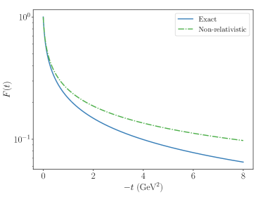
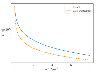
Figure 2: Form factors for a scalar toy model with deuteron-like kinematics. Exact results for (left panel) $F(t)$ and (right panel) $D(t)$ are compared to their non-relativistic approximations.

In Fig. 2, we compare the exact relativistic electromagnetic form factor $F(t)$ and exact stress form factor $D(t)$ to their non-relativistic approximations $F_{\mathrm{NR}}(t)$ and $D_{\mathrm{NR}}(t)$ as functions of $-t$. The derivation of the exact and non-relativistic form factors serves as a rough guide for the significance of relativistic effects in the system.

The exact and non-relativistic $F(t)$ are close when $-t/M^{2}<0.1$ (or $-t\approx 0.4$ GeV²), but diverge significantly at moderate and larger $-t$. Since $D(0)$ is not protected by a conservation law (unlike $F(0)$ or $A(0)$), it is possible for the exact and non-relativistic values to differ. Indeed we find an exact D-term value of $D(0)=-3.74$ and a non-relativistic value of $D_{\mathrm{NR}}(0)=-3.67$, which are fairly close in magnitude, but non-negligible. The differences between the exact and non-relativistic form factors illustrate the differences discussed in Eq. (33) and related paragraphs.

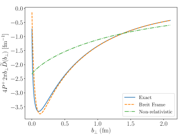
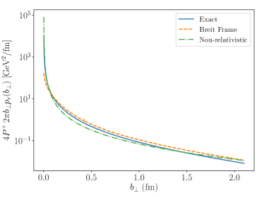
Figure 3: $D$-term related densities for a scalar toy model with deuteron-like kinematics. Exact results, Breit frame results, and non-relativistic approximations for (left panel) the potential $\widetilde{D}(b_{\perp})$ and (right panel) the 2D radial pressure $p_{r}(b_{\perp})$ are compared.

Next, we compare the densities entailed by the relativistic and non-relativistic $D(t)$ in Fig. 3. In particular, the direct Fourier transform $\widetilde{D}(b_{\perp})$ [as defined in Eq. (15)] and the radial pressure are both examined. For spin-zero targets, the Breit frame pseudo-density additionally differs from both the exact light front result due to the appearance of the factor $1/\sqrt{1-t/4M^{2}}$, so it is compared to the exact and non-relativistic results in both cases.

In the left panel of Fig. 3, the areas under the exact and Breit frame curves are the same, since the two-dimensional integrals of Eq. (15) and Eq. (70) are equal. However, the factor $1/\sqrt{1-t/4M^{2}}$ in Eq. (70) leads to the suppression of $\widetilde{D}_{\mathrm{BF}}(b_{\perp})$ at small values of $b_{\perp}$ and enhancement at moderate values, both by small amounts. At large values, the densities become equal, showing the corrections related to the factor $1/\sqrt{1-t/4M^{2}}$ become negligible at large distances. However, the non-relativistic result for $\widetilde{D}(b_{\perp})$ is significantly different from the exact and Breit frame results, suggesting that relativistic effects may persist in mechanical densities even at fairly large distances.

This same trend can be seen in the radial pressure, as depicted in the right panel of Fig. 3. Relativistic effects propagate to large $b_{\perp}$, even when they would be expected to vanish. This occurs because the pressure does not correspond to a conserved current, and is thus sensitive to the details the dynamics of a system (see Refs. Hudson and Schweitzer (2018); Freese and Cloët (2019) for examples of cases where the details of dynamics are significant). The details of the dynamics affect the overall mechanical structure of the hadron, and not just local aspects of the structure at small distances. Note that the log scale in the right panel of Fig. 3 covers more than six orders of magnitude, so that the apparently small differences are actually rather large.

For a slightly more detailed perspective, consider the right hand side of Eq. (65), which was used in obtaining the relativistic $\widetilde{D}(b_{\perp})$. The matrix element is weighted by a factor $\frac{1}{x}$ compared to the matrix elements for the densities associated with $F(t)$ and $A(t)$. This factor increases the integrand when $x\sim 0$ or $x\sim 1$, conditions that are explicitly discounted by the non-relativistic limit in which (for equal mass constituents) we make the replacement $\frac{1}{x}\mapsto\frac{1}{\alpha}\approx 2$.

The overall lesson of this case is that, because the mechanical properties of a hadron are not protected by a conservation law, they are sensitive to the details of dynamics, and accordingly non-relativistic effects can have a significant effect even at large distances and even for weakly bound systems.

IV.3.2 Pion-like kinematics

We now consider the scalar toy model with kinematics appropriate for a constituent quark model of the pion. We use a “quark” mass of 210 MeV, which leads to an excellent description of the pion’s electromagnetic form factor Chung et al. (1988). With $M=140~{}MeV$, this means that $B/M=2$, and according to Eq. (86) we get $D_{\mathrm{NR}}(0)=-1$, a result that immediately demonstrates the importance of relativistic effects for this model.

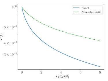
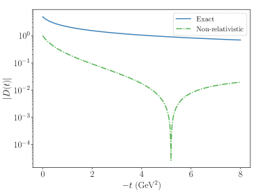
Figure 4: Form factors for a scalar toy model with pion-like kinematics. Exact results for (left panel) $F(t)$ and (right panel) $D(t)$ are compared to their non-relativistic approximations.

In Fig. 4, we present the exact and non-relativistic form factors $F(t)$ and $D(t)$. As expected, the relativistic effects are substantial. Even at $t=0$, we have $D(0)=-4.9$ and $D_{\mathrm{NR}}(0)=-1$, about a fifth of the true value. Moreover, the non-relativistic approximation of $D(t)$ as a zero crossing that’s absent in the exact result, as seen in the right panel of Fig. 4. This is because of the increasing importance of $z$ values near $\frac{1}{2}$ with larger $\Delta^{2}$, which causes the second term in the integrand of Eq. (85c) to dominate over the first term.

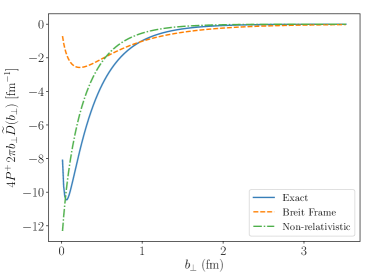
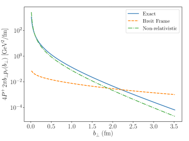
Figure 5: $D$-term related densities for a scalar toy model with pion-like kinematics. Exact results, Breit frame results, and non-relativistic approximations for (left panel) the potential $\widetilde{D}(b_{\perp})$ and (right panel) the 2D radial pressure $p_{r}(b_{\perp})$ are compared.

The density $\widetilde{D}(b_{\perp})$ and radial pressure are shown in Fig. 5. As expected, there are very substantial differences between the true density, Breit frame pseudo-density, and non-relativistic approximation. Remarkably, the Breit frame result is a worse approximation to the true density in this case than the non-relativistic approximation. This demonstrates the significance of the extraneous factor $1/\sqrt{1-t/(4M^{2})}$ present in the Breit frame densities, and strongly forces us to the conclusion that the findings of Refs. Panteleeva and Polyakov (2021); Kim and Kim (2021) cannot be applied outside of the spin-half case, where those results hold only by accident.

V Summary and conclusions

In this work, we obtained exact relativistic (light front) and approximate non-relativistic expressions for densities in spin-zero in spin-half hadrons. Focus was placed on the $P^{+}$ and mass densities, as well as the pressures encoded by the stress tensor as seen from the perspective of an observer comoving with the hadron. We compared the exact and non-relativistic expressions to those obtained in the Breit frame formalism. We find that, in general, the Breit frame densities do not have a direct correspondence with the exact light front densities, even through Abel transforms. This failure of correspondence occurs in the spin-zero case because of an extraneous factor $1/\sqrt{1-t/(4M^{2})}$ present in the integrand of every spin-zero Breit frame density, and in both cases because the relativistic light front densities do not exhibit spherical symmetry. The latter of these facts is illustrated for spin-half hadrons in particular by the azimuthal dependence of $P^{+}$ densities and pressures of transversely polarized states, to which the inverse Abel transform is inapplicable even formally. In general, however, the light front formalism lacks spherical symmetry, since there is no $\mathrm{SO}(3)$ subgroup of the Poincaré group that commutes with $P^{-}$ Brodsky et al. (1998).

The significance of both relativistic effects and the extraneous term $1/\sqrt{1-t/(4M^{2})}$ present in the spin-zero Breit frame densities is illustrated through a pedagogical model. Relativistic effects were found to affect the mechanical structure of a composite system significantly, even for weakly bound systems and at large distances—in contrast to the electromagnetic density or mass density, both of which are protected by conservation laws. Moreover, for strongly bound systems, we found that the extraneous factor $1/\sqrt{1-t/(4M^{2})}$ makes the (Abel transform of the) Breit frame density a poor approximation to the true density.

Taking the inverse Abel transform of a transverse light front density can, at best, return a partially non-relativistic approximation. This approximation is partially non-relativistic, since a non-relativistic approximation of the internal dynamics has not been applied to the form factors associated with the density, but instead only to the accompanying Lorentz tensors. In some circumstances, such as neutron star structure, this approximation may be warranted (cf. Ref. Rajan et al. (2018) for an example of this application), but one should bear in mind that this operation is an approximation that eliminates effects due to boosts from the target’s rest frame. For targets with wave functions localized to a smaller distance than their reduced Compton wavelength, or targets for which a finer resolution of internal structure than the Compton wavelength is desired—such as hadrons—this approximation cannot be justified.