Iterative Symbolic Regression for Learning Transport Equations

Abstract

Computational fluid dynamics (CFD) analysis is widely used in chemical engineering. Although CFD calculations are accurate, the computational cost associated with complex systems makes it difficult to obtain empirical equations between system variables. Here, we combine active learning (AL) and symbolic regression (SR) to get a symbolic equation for system variables from CFD simulations. Gaussian process regression-based AL allows for automated selection of variables by selecting the most instructive points from the available range of possible parameters. The results from these experiments are then passed to SR to find empirical symbolic equations for CFD models. This approach is scalable and applicable for any desired number of CFD design parameters. To demonstrate the effectiveness, we use this method with two model systems. We recover an empirical equation for the pressure drop in a bent pipe and a new equation for predicting backflow in a heart valve under aortic insufficiency.

Introduction

Computational fluid dynamics (CFD) provides a numerical approximation to the conservation of mass, momentum and energy (Navier-Stokes equations) that govern the fluid flow behavior. While experimentally quantifying fundamental mechanisms of a process is often insightful, CFD modeling can provide an alternative approach for better understanding of the underlying physics in a less resource-intensive manner¹. With continued growth of computational power and advances in CFD techniques, even complex models can be done on commodity hardware. Thus, CFD modeling is routinely applied in several fields of science and engineering such as chemistry^{2; 3}, materials⁴, fluid flow and heat transfer^{5; 6}, biology⁷, drug delivery⁸, semiconductors⁹, environmental engineering ^{10; 11}, biomedical engineering¹² and aeronautics¹³.

Parametric analysis has been widely used in process modeling and design optimization using a semi-automated or fully-automated workflows^{14; 15; 16}. However, running the entire CFD calculations on all possible design parameters can be computationally expensive, especially for complex CFD models. Thus, there is a need to identify which feature points are most important in experiment design, and allow for system analysis with fewer CFD simulations. Another challenge in the mentioned settings is the lack of quantitative general equations that can be applied to different systems. This includes different geometrical designs, as well as having different operating conditions such as temperature, pressure, velocity or fluid properties. These system variables that can be inputs to CFD models are referred to as feature points in this work.

Here, we apply active learning (AL) to CFD modeling experiment design and then use symbolic regression (SR) to find empirical symbolic equations for these CFD models. AL is an iterative supervised learning technique that attempts to learn a good model from a few data points, by allowing the model to pick which data points it trains from.¹⁷ In other words, AL is the process of choosing the next experiment or feature point optimally using less resources and adding this new point to the training data. In this paper, we use AL with gaussian process regression (GPR) to choose the next optimal CFD feature points. GPR is often associated with Bayesian optimization, where the goal is to optimize an expensive black box function. However, our goal is to find a symbolic equation across all feature values rather than a single optimum with as few CFD simulations as possible.

SR is a machine learning approach used to systematically determine symbolic equations that fit certain data with an unknown underlying function.^{18; 19; 20} Unlike regression, where data is fit to a pre-defined function, SR attempts to find both the model and model parameters simultaneously. Neural networks (NN) are a popular choice for learning from data. However, even though they can approximate any function, the output from neural networks is difficult to interpret and cannot be converted to an analytical function. SR gives interpretable symbolic equations from data, which makes this approach appealing. Here, “interpretable” means that the exact relationship between input features and outputs is known in equation form. There are limited studies that explore SR to find general relationships from CFD simulations.^{21; 22} In this study, we demonstrate the use of AL for design of CFD experiments, and then apply the SISSO SR method to determine the physics of fluid systems. Figure 1 provides an overview of this method. A fully-automated workflow is combined with AL to generate CFD data, which is then used to get an empirical symbolic equation using SR. To avoid non-physical symbolic equations, we include known asymptotic points using prior understanding of physics of the fluid systems being studied. These asymptotic points are included in the SR training data. This forces SR to return equations have the correct asymptotic behavior at extreme geometries and velocities. The AL and SR methods are described in detail in sections that follow.

Comparison to Related Work

Previous studies have implemented AL to accelerate simulation-driven design optimization. Owoyele et al. ²³ used AL to perform simulation-based data generation, ML learning and surrogate optimization to refine solution in the vicinity of predicted optimum parameters for design of a compression ignition engine. Gonçalves et al. ²⁴ studied the generation of simulation-based surrogate models with the task of parameter domain exploration using various sampling and regression-based AL strategies. In a similar work, Pan et al. ²⁵, used AL for developing surrogate models for industrial fluid flow case studies under a constraint of a limited function evaluations. AL has also been implemented in specific experiment design to deploy efficient design space exploration to enhance model quality.^{26; 27}. Over the past few decades, multiple methods to solve the SR problem have been developed. Traditional deterministic algorithms assume a predefined mathematical function and attempt to find parameters with the best fit to the data, whereas, evolutionary algorithms try to find parameters and learn the best-fit function, simultaneously. Some prevalent methods are genetic programming algorithms ^{28; 29; 30; 31; 32; 33; 34}, sparse regression ^{20; 35; 36; 37}, pareto-optimal regression ^{38; 39}, and the sure-independence screening and sparsifying operator (SISSO) method.^{40; 41} Most SR frameworks implement the popular Genetic programming, ⁴² which is an improved version of Genetic Algorithms (GA), ^{43; 44} inspired by Darwin’s theory of natural selection. Genetic programming has also been used to identify hidden physical laws from the input-output response prior.^{45; 46; 47} We use SISSO because it has been shown to be robust with small amounts of data.^{40; 48; 49} This is advantageous for analysis of CFD systems where the computational cost of simulations increases with increasing number of variables and complexity of the system. Compared to existing work, our approach is novel in the sense of combining AL and SR to optimize training efficiency and output a general equation for any fluid system of interest.

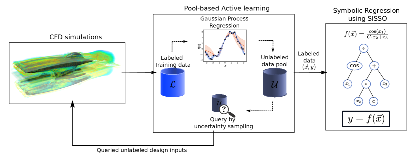
Figure 1: Process overview. A fully automated parameterized CFD model is coupled with pool-based active learning (AL). The CFD model is used to generate the labeled training data. The AL model is used to predict the next feature point for CFD simulations. An iteration of AL consists of learning the available data using gaussian process regression and then using uncertainty sampling to find the next feature point to label using a CFD simulation. The labeled data is then used as training data for symbolic regression to find the empirical symbolic equation for CFD feature inputs and outputs.

Theory

Governing Equations

The governing equations are the conservation of mass, momentum and energy. With the assumption of steady state, incompressible flow and constant temperature, we have the continuity equation:

$$\nabla.\vec{v}=0$$ (1)

and the momentum equation can be simplified to:

$$\rho(\vec{v}.\nabla)\vec{v}=-\nabla P+\mu\nabla^{2}\vec{v}$$ (2)

where, $\vec{v}$ is the velocity vector, $P$ is pressure and $\rho$ and $\mu$ denote the fluid density and viscosity, respectively. A Dirichlet boundary condition is imposed at the inlet, with a parabolic velocity profile normal to the boundary for all cases. This assumption allows the analysis for a fully-developed flow without the need for unnecessary geometry extensions, which results in extra mesh elements. The no-slip boundary condition imposed at the wall ensures a zero velocity relative to the pipe surface. Given the unknown pressure at the outlet, the outflow boundary condition is imposed. A convergence criterion is defined based on the conservation of mass at the inlet and outlet boundaries.

Pressure Drop in a Bent Pipe

The laminar fluid flow in circular pipes is a classical problem in fluid mechanics, and it has been analyzed by the means of momentum balance, resulting in the famous Hagen-Poiseuille (HP) equation ⁵⁰:

$$w=\frac{\pi(P_{0}-P)d^{4}\rho}{32\mu L}$$ (3)

where the mass flow rate $w$ is the product of cross-sectional area, density and average velocity $\langle v\rangle$. Here $d$ and $L$ are the pipe diameter and length, respectively, and $P_{0}$ and $P$ denote the pressure at the inlet and outlet of the pipe. Note that Equation 3 is only valid for continuous, laminar, incompressible, steady, Newtonian flow that is fully-developed. Given the pipe dimensions, fluid properties and average inlet velocity, one can easily obtain the pressure drop using Equation 3. Our goal here is to find an empirical equation for the pressure drop in a bent circular pipe as a function of the average inlet velocity ($\langle v\rangle$), pipe diameter ($d$) and bend angle ($\theta$). The fluid is considered to be water at 25 ^∘C with constant properties. This setting is implemented to limit the number of feature points to three. However, more complicated models involving chemical reactions and convective heat transfer can be analyzed with more feature points. The geometry has been parameterized and meshed with hexahedral elements, as represented in Figure 2. More details on model parameterization can be found in Section LABEL:section1.1 of Supplementary Information (SI).

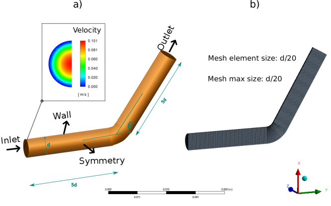
Figure 2: Bent pipe: a) parameterized geometry with inlet, wall, symmetry and outflow boundary conditions. A parabolic velocity profile is defined normal to the boundary to satisfy the assumption of fully-developed flow. The geometric constraints allow having different user inputs for $d$ and $\theta$ and ensure valid geometries. b) parameterized hexahedral mesh with element size and max element size of $d$/20, which allows for adjustable meshing given different geometric inputs for $d$ and $\theta$.

Using Equation 3, the model is validated based on 5 different inputs with a bend angle of 1^∘, which is approximately equivalent to a straight pipe. The mean error for the unit length pressure drop with respect to the HP equation is about 2$\%$.

Backflow at an Expansion Joint

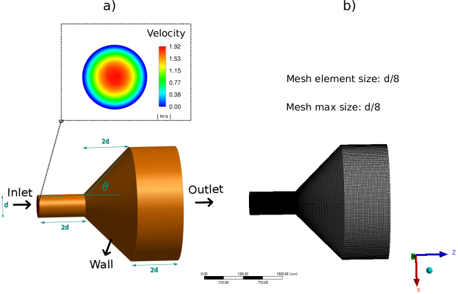
Figure 3: Expansion joint: a) parameterized geometry with inlet, wall and outflow boundary conditions. A parabolic velocity profile is defined normal to the boundary to satisfy the assumption of fully-developed flow. The geometric constraints allow having different user inputs for $d$ $\theta$ and ensure valid geometries. b) parameterized hexahedral mesh with element size and max element size of $d$/8, which allows for adjustable meshing given different geometric inputs for $d$ and $\theta$.

We can consider the human heart to operate as two pumps in series. The right heart pumps blood to the pulmonic circulation and the left heart to the systemic circulation⁵¹. The valves in the human heart open and close efficiently, allowing the blood flow in the forward direction and minimizing the regurgitation of flood to the chamber it came from. Aortic insufficiency is a condition in which the heart valve fails to tightly close, allowing blood to flow backwards into the heart instead of pumping out ⁵². We have considered an expansion joint to simulate this condition in a simplified geometry and quantify the backflow volume. The fluid is blood with constant properties with density and viscosity set to 1060 Kg/m³ and 0.004 Pa s at 37^oC. A fully-developed flow is defined at the inlet boundary, no-slip velocity at wall and outflow boundary condition at the outlet. The inlet pressure is set to 120 mmHg absolute. Once again, the geometry and the hexahedral mesh are constrained to avoid invalid models given different inputs (see Figure 3). Blood dominantly flows in the $z$ direction, thus the $z$ component of the velocity is used as our metric for defining the backflow. The backflow volume is calculated by summing over the volume of mesh with negative velocity in $z$ direction (see SI Section LABEL:section1.2). The inputs to the model in this setting are the average inlet velocity ($\langle v\rangle$), inlet diameter ($d$) and expansion angle ($\theta$). The model outputs the percentage backflow ($f$) by finding the ratio of $V_{bf}$ to the total system volume.

Active Learning Model

The goal of AL algorithms is to increase accuracy of a machine learning model, while minimizing the training data required to train the model. It is often formulated as an optimization problem.¹⁷ Here, we use a pool-based AL setting. Pool-based AL assumes that the model has access to a large set of unlabeled samples. Consider a dataset $\mathcal{D}\supseteq\{\mathcal{L},\mathcal{U}\}$ comprised of a small set of labeled data $\mathcal{L}=\{(\vec{x}_{i},y_{i})\}_{i=1}^{n_{\mathcal{L}}}$ with features $\vec{x}_{i}$ (n-dimensional vector) and corresponding labels $y_{i}$, and a large pool of unlabeled data $\mathcal{U}=\{\vec{x}_{j}\}_{j=1}^{n_{\mathcal{U}}}$ containing only features $\vec{x}_{j}$. $n_{\mathcal{L}}$ and $n_{\mathcal{U}}$ are the number of samples in the labeled and unlabeled dataset, respectively, and $n_{\mathcal{L}}\ll n_{\mathcal{U}}$. A model $\Phi$ is initially trained using the labeled data $\mathcal{L}$. Next, an unlabeled data sample, called a query, $\vec{x}_{i+1}$ is selected from the unlabeled data pool $\mathcal{U}$ using a query strategy. The selected query is then labeled by using an “oracle”. An oracle is a human expert, or an experiment, but in this work it is a CFD simulation. The label $y_{i+1}$ is found by conducting a CFD simulation for the flow conditions and geometry specified by $\vec{x}_{i+1}$. This new observation $(\vec{x}_{i+1},y_{i+1})$ is added to labeled data $\mathcal{L}$ and the model $\Phi$ is retrained based on this updated value. The process of query-label-retrain is iteratively repeated until the labeling budget is exhausted.

In this study, we use gaussian process regression⁵³ (GPR) as our predictive model $\Phi$ and uncertainty sampling⁵⁴ as the query strategy. The uncertainty sampling strategy selects the feature point whose prediction is most uncertain. The model has the least information in the vicinity of the most uncertain prediction, and it is relatively more confident about other predictions. Hence, labeling the most uncertain point is most informative for the model.^{17; 55} GPR is a probabilistic estimation method and has the ability to provide uncertainty measurement because it provides confidence intervals for predictions at each feature point. The goal of any regression model is to fit a function to datapoints. There are infinitely many functions that can possible fit a set of points. GPR assigns a probability to each of these functions.⁵⁶ Once the GPR model $\Phi$ is trained, the uncertainty in predictions and next feature point choice are calculated using Equations 4 and 5:

$$U(\vec{x})=\left[1-\max\left(P^{i}_{\Phi}(y|\vec{x})\right)\right]$$ (4)

$$\vec{x}_{i+1}=\operatorname*{\arg\!\max}_{x}U(x).$$ (5)

To ensure the method is robust to label noise, $U(x)$ is itself made a probability and $x_{i+1}$ is sampled rather than computing the $\operatorname*{\arg\!\max}$. This is accomplished by computing the softmax of the predicted uncertainty, $U(x)$.⁵⁷ Thus, our AL equation is

$$P(\vec{x}_{i+1})=\mathrm{softmax}[U(\vec{x})]=\frac{e^{U(x)_{j}}}{\Sigma_{j=1}^{n_{\mathcal{U}}}U(x)_{j}}$$ (6)

Readers are referred to Section LABEL:sectionAL of the SI for further details.

Symbolic Regression Model

To learn an interpretable model from CFD simulations, we use SISSO, developed by Ouyang et al. ⁴⁰ SISSO aims to construct a symbolic equation between primary features $\vec{x}$ and labels $y$. Given M samples, SISSO assumes that the labels can be expressed as a linear combination of non-linear functions of primary features. So, $y=f(\Psi)$ where $\Psi=\{\psi_{1},\psi_{2},...,\psi_{r}\}$ is a set of secondary features. The secondary features $\psi_{i}$ are non-linear, closed form functions of primary features. If $\vec{x}=[x_{1},x_{2},x_{3},...,x_{n}]$ are primary features, then examples of secondary features are $\{x_{1}/x_{3},\ x_{3}-x_{1}x_{2},\ x_{4}x_{5}/x_{1},...\}$. These secondary features are obtained by recursively applying a set of user-defined operators on the primary features and creating a set of potential secondary features. The operator set can be any combination of unary and binary operators. The number of potential secondary features is proportional to the number of primary features used, the number of operators used, and the level of recursion. At each iteration, SISSO selects the subsets of secondary features that have the largest linear correlations with $y$. The number of terms in the linear expansion $f(\Psi)$ (called descriptors) are controlled by a sparsifying $l_{0}$ regularization. Note, here the number of descriptors refers to the number of terms in the output equation. For each iteration $q$, SISSO constructs multiple models for $f(\Psi)$ using the secondary features and selects the one with the largest correlation with the target property. More details on this procedure can be found in Ouyang et al. ⁴⁰

In SISSO, dimensional analysis is performed to retain only valid combinations of primary features. This ensures that secondary features do not have unphysical units (e.g. force + time). To achieve this, there is an option in SISSO to group primary features that have the same derived units. We modified this option so that the primary features are expressed in terms of fundamental units of measurement (mass, length, time, angle) and grouped based on these fundamental units instead of derived units.

Methods

In this section, the fully-automated CFD workflow, AL and symbolic regression procedures are explained. As seen in Figure 1, we first use AL to get labeled data from the CFD model and then perform SR using that as training data, to obtain an empirical symbolic equation between features and labels.

Our fully-automated workflow has been used on two different fluid flow problems, as described in previous sections. These problems are not necessarily complex, and the main goal here is to demonstrate a more robust approach that can also be applied to complex problems. In this work, we have coupled ANSYS Workbench with python. The parameterized CFD models are developed by defining input feature points. These inputs can include geometric features, operating conditions and fluid flow properties. They are easily adjustable in a python script and the outputs are updated accordingly.

Table 1: Feature ranges and test data split for the two systems.

System		Features		Labels	Test data	Data Split (train:test counts)
	$d$ (m)	$\theta\ (^{\circ})$	$\langle v_{in}\rangle$ (m/s)
Bent pipe	$0.005-0.1$	$1-180$	$0.005-0.02$	$\Delta P/L$	$d>0.07$m and $\theta>120^{\circ}$	3696:400
Expansion joint	$0.0005-0.005$	$15-60$	$0.002-0.5$	$f$	$d>0.0025$m and $\theta>50^{\circ}$	1764:589

For both the systems described preciously, we have 3-dimensional (3D) features, meaning we vary are 3 input parameters for the CFD simulations. For the bent pipe system, these features are pipe diameter ($d$), bend angle ($\theta$), and average inlet velocity ($\langle v_{in}\rangle$). For the expansion joint, features are inlet pipe diameter ($d$), expansion angle ($\theta$) and average inlet velocity ($\langle v_{in}\rangle$). The target property $y$ for bent pipe is pressure drop $\Delta P/L$ and for the expansion joint, it is the backflow volume percentage $f$. To start with, a range of acceptable values for the input parameters is chosen to ensure laminar fluid flow and the 3D feature space is divided into training data and testing data. The ranges for features and test/train split criteria are shown in Table 1. Since we are not tuning hyperparameters, we do not use a validation split. To make sure that physics of the system are obeyed, we define asymptotes based on prior system knowledge. In the bent pipe system, $d=0$ will result infinite pressure drop ($\displaystyle{\lim_{d\to 0}\frac{\Delta P}{L}(d,\theta,v)=\infty}$), which is a valid asymptote as per the HP equation (Equation 3). Parameter $\theta$ is set to be bounded between $15-60^{\circ}$ in the expansion joint system. The rationale behind this choice comes from the fact that no backflow is formed at smaller expansion angles, which results a zero variance in the labels for all possible variations of the other two features ($f(d,\theta,v)\Big{|}_{\theta<15^{\circ}}=0;\forall d,v$). On the other hand, at larger angles beyond this limit, the size of the system increases significantly as a result of geometrical constraint set for the length of the expansion section (see Figure 3). Specifically, for the case of $\theta=90^{\circ}$, the system size becomes infinite as a result of having an infinite outlet diameter.

For AL, three random points $\vec{x}$ from the training data are sampled, and CFD simulations are generated to find corresponding labels $y$. This is our initial training data ($\mathcal{L}$) for our pool-based AL and the rest of the feature points form the unlabeled data pool $\mathcal{U}$. CFD simulations are used to label data for feature points obtained from Equation 6. After $N$ such queries, feature-label pairs in $\mathcal{L}$ are used as training data for the SISSO algorithm. We then add asymptotic points to this training data. The number of asymptotic points added depends on the number of training data points $N$ in $\mathcal{L}$. We add greater of 3 or 10% of $N$ points to $\mathcal{L}$ and make sure that all asymptotic conditions are represented. To create aymptotic data points, the primary features apart from the variable for which the aymptote is defined are sampled randomly from the regime defined for that feature. So, for the bent pipe system, when $\displaystyle{\lim_{d\to 0}\frac{\Delta P}{L}(d,\theta,v)=\infty}$, $\theta$ and $\langle v_{in}\rangle$ are randomly sampled from the bounds defined in Table 1. Density and Viscosity are also added as features for SISSO. We use the operator set $\{+,-,\times,\div,\exp,-\exp,()^{-1},()^{2},\sin,\cos\}$ with our features for both systems and set the number of descriptors to 3. The symbolic equation obtained from SISSO is used to predict labels for the test features. This method is compared against random search and grid search experiment design algorithms. Random search is random selection of feature points with uniform sampling probability from the data pool. Grid search is when a hypercube of points from the 3D feature grid are selected. Grid is equivalent to a factorial design if we view our levels as discretization of our features. SISSO is used to find equations for both these methods so they can be compared against our AL + SISSO method. The difference in these methods is reported using significance statistics obtained from an independent samples t-test. The independent samples t-test is a parametric test that compares the means of two independent distributions and gives statistics to confirm the hypothesis that the two populations are significantly different.⁵⁸

Results and Discussion

The method described above, AL + SISSO, is tested and compared with baseline methods used for experiment design like random search and grid search. The objective was to obtain a symbolic relationship between inputs/features and outputs/labels, given data.

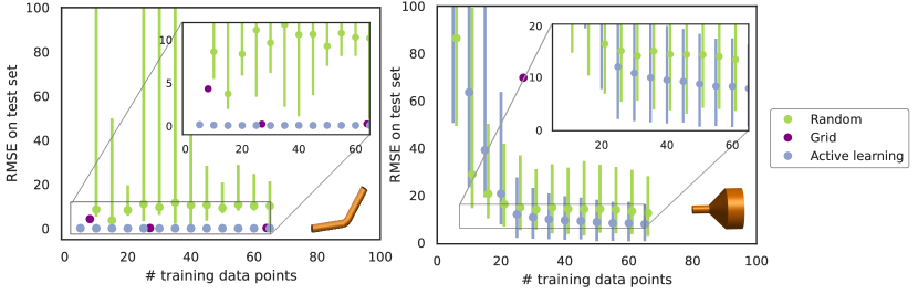
Figure 4: Root mean squared errors (RMSE) as a function of number of training data points. The symbolic regression equations obtained from different models for varying number of training data points are evaluated for test data and the RMSE in predictions is plotted. Error bars on these points indicate the 50^th quantile for RMSEs on test data. It is observed that AL model for experiment design has the best performance followed by random selection of experiment points. A grid search model requires many data points to achieve comparable performance.

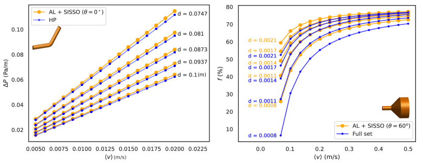
Figure 5: Comparison of SISSO results with baseline models.

In Figure 4, we compare the root mean squared error (RMSE) on test data from SR equations for AL, random search and grid search. The symbolic relationships obtained from SISSO for AL, random search and grid search are evaluated on the test data points and respective RMSEs are calculated between these values and actual CFD values. Test data was withheld from the training data pool for both systems, as shown in Table 1. In Figure 4, each data point for AL and random search represents the mean value for RMSE from 100 independent iterations of training data sampling followed by SISSO. The uncertainty in AL comes from the randomly sampled initial training points and is in the coefficients $C_{i}$ of SISSO equations. For bent pipe, we observe that AL converges quickly and requires fewer training points to get an accurate symbolic equation between features and labels. RMSEs for random search and AL are significantly different ($p=8.8\times 10^{-23}$, via independent samples t-test). Grid search outperforms random search and requires 27 training points to converge. Table LABEL:tab:system1 shows some equations obtained from SISSO for AL, random search, grid search and the full training set. The complete list of equations obtained for different methods, as a function of training data points, is reported in Table LABEL:tab:system1_si. The equations reported are those that are observed maximum times (mode of the distribution) for a given value of training points. AL combined with SISSO provides an accurate equation with as low as 10 training data points, and the general form of the equation remains the same with increasing training data points. Random search requires 15 training points to obtain a similar equation. The equation obtained for grid search varies with increasing training points. Although, random search obtains the correct general equation with few points, the variance in the coefficients for these equations is high and hence, have a high RMSE in their approximation of pressure drop in the system. For the expansion joint, AL outperforms random search and grid search. The difference in RMSE between AL and random search increases as the number of training points increases ($p=0.0125$, via independent samples t-test). Equations obtained from SISSO for this system are reported in Table LABEL:tab:system2 and the complete list as a function of training data points can be found in Table LABEL:tab:system2_si. The general equation for AL, random search and grid search remains the same after 30, 60 and 512 training points, respectively.

We also compare the performance of AL + SISSO models with baseline models. Figure 5 shows how AL + SISSO compares to the respective baseline models. At $\theta=0^{\circ}$, the bent pipe becomes a straight pipe, for which $\Delta P/L$ can be calculated using the HP equation (Equation 3) and is considered the baseline. AL + SISSO equation results fit the HP equation. For backflow in the expansion joint, there is no such theory-derived equation to compare against. So, we perform SISSO on the entire feature pool and consider that as the baseline model. AL + SISSO predictions for $\theta=60^{\circ}$ underestimate the backflow percentage compared to the baseline. However, the curves for AL + SISSO follow the same form as the baseline and there is an offset along the y-axis. SISSO equations obtained for AL and the baseline are the same, and the difference in predicted labels comes from the coefficients C1, C2, C3 for the two equations. This is reasonable since our goal is to find a symbolic equation to understand the system and not to minimize the regression error.

In the final analysis, it is important to consider how well the results of AL+SISSO can be used to describe flow and how well they compare to known equations when they exist. In the case of the bent pipe, the data in Figure 5 confirms that the AL+SISSO matches nearly exactly with the HP Equation. Note that all symbolic equations beyond 10 training points shown in Table LABEL:tab:system1_si are consistent with theory-driven HP equation (Equation 3) for $\theta=0$ and accurately describe the pressure drop in the system. When known equations do not exist, which is the case for most complex flow scenarios, the ability of AL+SISSO to describe flow needs to be carefully interpreted and compared to best known approximations. For the expansion joint, there are no accepted equations for the backflow volume percentage to compare against for any geometry, so comparisons are made with the entire feature pool referred to as the full set in the figure. The data in Figure 5 does show a difference between the AL+SISSO and the full set. The important observation is that the shape of the graph for the volume percentage versus velocity are quite similar, rising and then leveling off with velocity as one would expect. The observed difference is the result of the coefficients in the equations as mentioned above and not an incorrect symbolic equation.

Conclusions

We introduce an AL approach combined with SR for obtaining an empirical symbolic relationship between system variables for CFD simulations. This framework eliminates the need for the conventional trial-and-error or grid search methods for picking feature points since we let AL pick these points based on prior information available. We demonstrate the use of this method for two CFD systems and compare them against conventional methods. The results obtained from SISSO are more interpretable than those obtained from black box functions, and can be directly used. This method also greatly reduces the amount of data needed to get meaningful insights about a CFD system. One limitation of this method is that the obtained symbolic relationships are only valid for fluid flow regimes described by the feature domain considered for the training data pool (i.e. laminar flow regime for the two examples illustrated). Augmenting training data with asymptotic points from prior scientific knowledge helps ensure that the equations obey the physics of the system.

Table 2: Equations obtained from SISSO for the Bent Pipe system

Method	Training Points	Mean Test RMSE	Equation
AL	5	0.143	$\frac{C_{1}v+d\left(C_{2}v\sin{\left(\theta\right)}+C_{3}\theta\cos{\left(\theta\right)}\right)}{d^{2}}$
Random	5	349.42	$\frac{C_{1}\cos{\left(d\right)}}{d^{2}}+\frac{C_{2}e^{-v}}{d^{2}}+\frac{C_{3}\theta v^{2}}{d}$
Grid	8	4.32	$\frac{C_{1}v}{d^{2}}+\frac{C_{2}\theta^{2}v}{d}-C_{3}e^{v}+C_{3}e^{-\theta}$
AL	60	0.072	$\frac{v\left(C_{1}+C_{2}\theta+C_{3}d\theta v\right)}{d^{2}}$
Random	60	10.29	$\frac{v\left(C_{1}+C_{2}\theta+C_{3}d\theta v\right)}{d^{2}}$
Grid	64	0.246	$\frac{C_{1}v+C_{2}d\theta v^{2}+C_{3}\theta^{2}}{d^{2}}$
Full set	3696	0.085	$\frac{v\left(C_{1}+C_{2}\theta+C_{3}d\theta v\right)}{d^{2}}$

Table 3: Equations obtained from SISSO for the Expansion Joint

Method	Training Points	Mean Test RMSE	Equation
Random	5	86.42	$C_{1}v\sin{\left(\theta\right)}+C_{2}\theta ve^{d}+C_{3}de^{d}$
AL	5	107.13	$C_{1}\sin{\left(\theta\right)}+\frac{C_{2}\theta}{v\sin{\left(d\right)}}+C_{3}\sin{\left(\frac{\theta}{d}\right)}$
Grid	8	4955.92	$\theta\left(C_{1}v\sin{\left(\theta\right)}+C_{2}d\theta v+\frac{C_{3}d}{\cos{\left(d\right)}}\right)$
AL	60	8.25	$\frac{\theta\left(C_{1}dv\cos{\left(\theta\right)}+C_{2}+C_{3}\theta\right)}{dv}$
Random	60	13.30	$C_{1}e^{-d\theta}+C_{2}e^{\theta}+C_{2}e^{-\theta}+C_{3}dve^{-d}$
Grid	64	79.35	$C_{1}d\theta e^{-d}+C_{2}d^{3}v+C_{3}\sin{\left(\theta\right)}$
Full set	1764	12.65	$\frac{C_{1}\theta dv\cos{\left(\theta\right)}+C_{2}dv\sin{\left(d\theta\right)}+C_{3}}{dv}$

S1 CFD Models Methods

S1.1 Bent Pipe System

By cutting the geometry in half, a symmetrical boundary condition is imposed on the front interior face. To avoid invalid geometries, a set of parametric constraints are applied, where both inlet and outlet side extrusions have length of 5$d$. The reference point for the revolving bend is also set to be at a distance $d$ from the pipe center-line. Given the nature of our automated workflow, the mesh sizing is also constrained to $d/20$ which enables adjustable meshing based on the user input for the pipe diameter.

S1.2 Expansion Joint System

The inlet-side extrusion length, expansion height and outlet-side extrusion length are set to be 2$d$, while the expansion angle is $\theta$. The backflow volume is calculated by summing over the volume of mesh elements where $v_{z}<0$:

$$V_{bf}=\int_{V}\phi_{V}dV$$ (S1)

where $\phi$ is our user-defined function (UDF):

$$\phi_{V}=\begin{cases}1&\text{if }v_{z}<-0.0001\\ 0&\text{otherwise}\end{cases}$$ (S2)

Note that in Equation LABEL:eq:phi, the threshold is set to a small negative value (-0.0001 m/s), to avoid the inclusion of those mesh elements at the wall, where no-slip boundary is applied.

S2 Active learning Softmax Adjustment

When uncertainty prediction for AL uses argmax (Equation LABEL:eq:wo_softmax), the predictions are sensitive to noise in the labels. Figure LABEL:fig:without_softmax shows the RMSE on test data when softmax is not applied to AL prediction uncertainty.

$$\vec{x}_{i+1}=\operatorname*{\arg\!\max}_{x}\ \left[1-max\left(P_{\Phi}(\hat{y}|\vec{x})\right)\right]$$ (S3)

S3 Symbolic Regression Equations

Table 1: Equations obtained from SISSO for the Bent Pipe system

Method	Training Points	Mean Test RMSE	Equation
AL	5	0.143	$\frac{C_{1}v+d\left(C_{2}v\sin{\left(\theta\right)}+C_{3}\theta\cos{\left(\theta\right)}\right)}{d^{2}}$
Random	5	349.42	$\frac{C_{1}\cos{\left(d\right)}}{d^{2}}+\frac{C_{2}e^{-v}}{d^{2}}+\frac{C_{3}\theta v^{2}}{d}$
Grid	8	4.32	$\frac{C_{1}v}{d^{2}}+\frac{C_{2}\theta^{2}v}{d}-C_{3}e^{v}+C_{3}e^{-\theta}$
Random	10	8.63	$C_{1}v^{3}+C_{2}v^{3}+\frac{C_{3}\theta v}{d^{2}}$
AL	10	0.095	$\frac{v\left(\frac{C_{1}d}{\sin{\left(d\right)}}+C_{2}\theta+C_{3}d\theta v\right)}{d^{2}}$
Random	15	3.73	$\frac{v\left(C_{1}+C_{2}\theta+C_{3}d\theta v\right)}{d^{2}}$
AL	15	0.068	$\frac{v\left(\frac{C_{1}}{\sin{\left(d\right)}}+C_{2}\theta v+C_{3}d\theta^{2}v\right)}{d}$
AL	20	0.065	$\frac{C_{1}\sin{\left(v\right)}}{d^{2}}+\frac{C_{2}\theta v^{2}}{d}+C_{3}v^{2}e^{\theta}$
Random	20	8.36	$\frac{v\left(C_{1}+C_{2}\theta+C_{3}d\theta v\right)}{d^{2}}$
AL	25	0.075	$\frac{C_{1}\sin{\left(v\right)}}{d^{2}}+\frac{C_{2}\theta v^{2}}{d}+C_{3}v^{2}e^{\theta}$
Random	25	11.13	$\frac{v\left(C_{1}+C_{2}\theta+C_{3}d\theta v\right)}{d^{2}}$
Grid	27	0.22	$\frac{C_{1}v+C_{2}\theta^{2}+C_{3}d\theta v^{2}}{d^{2}}$
Random	30	9.65	$\frac{v\left(C_{1}+C_{2}\theta+C_{3}d\theta v\right)}{d^{2}}$
AL	30	0.061	$\frac{v\left(\frac{C_{1}d}{\sin{\left(d\right)}}+C_{2}\theta+C_{3}d\theta v\right)}{d^{2}}$
AL	35	0.071	$\frac{v\left(C_{1}+C_{2}\theta+C_{3}d\theta v\right)}{d^{2}}$
Random	35	11.77	$\frac{C_{1}\sin{\left(v\right)}+C_{2}\theta v+C_{3}d\theta v^{2}}{d^{2}}$
Random	40	10.59	$\frac{v\left(C_{1}+C_{2}\theta+C_{3}d\theta v\right)}{d^{2}}$
AL	40	0.083	$\frac{v\left(\frac{C_{1}d}{\sin{\left(d\right)}}+C_{2}\theta+C_{3}d\theta v\right)}{d^{2}}$
Random	45	10.65	$\frac{v\left(C_{1}+C_{2}\theta+C_{3}d\theta v\right)}{d^{2}}$
AL	45	0.066	$\frac{C_{1}\sin{\left(v\right)}}{d^{2}}+\frac{C_{2}\theta v^{2}}{d}+C_{3}v^{2}e^{\theta}$
AL	50	0.0822	$\frac{v\left(\frac{C_{1}d}{\sin{\left(d\right)}}+C_{2}\theta+C_{3}d\theta v\right)}{d^{2}}$
Random	50	9.28	$\frac{v\left(C_{1}+C_{2}\theta+C_{3}d\theta v\right)}{d^{2}}$
Random	55	10.78	$\frac{v\left(C_{1}+C_{2}\theta+C_{3}d\theta v\right)}{d^{2}}$
AL	55	0.075	$\frac{v\left(\frac{C_{1}d}{\sin{\left(d\right)}}+C_{2}\theta+C_{3}d\theta v\right)}{d^{2}}$
Random	60	10.29	$\frac{v\left(C_{1}+C_{2}\theta+C_{3}d\theta v\right)}{d^{2}}$
AL	60	0.072	$\frac{v\left(C_{1}+C_{2}\theta+C_{3}d\theta v\right)}{d^{2}}$
Grid	64	0.246	$\frac{C_{1}v+C_{2}d\theta v^{2}+C_{3}\theta^{2}}{d^{2}}$
AL	65	0.076	$\frac{v\left(C_{1}+C_{2}\theta+C_{3}d\theta v\right)}{d^{2}}$
Random	65	10.21	$\frac{v\left(\frac{C_{1}d}{\sin{\left(d\right)}}+C_{2}\theta+C_{3}d\theta v\right)}{d^{2}}$
Grid	125	2.92	$\frac{v\left(C_{1}+C_{2}d\theta v+C_{3}d^{3}\theta v\right)}{d^{2}}$
Random	125	9.91	$\frac{v\left(C_{1}+C_{2}\theta+C_{3}d\theta v\right)}{d^{2}}$
Grid	216	1.07	$\frac{v\left(C_{1}+C_{2}d\theta v+C_{3}d^{2}\theta^{2}\right)}{d^{2}}$
Random	216	9.97	$\frac{v\left(C_{1}+C_{2}\theta+C_{3}d\theta v\right)}{d^{2}}$
Grid	343	0.38	$\frac{C_{1}v}{d^{2}}+\frac{C_{2}v\sin{\left(\theta\right)}}{d}+\frac{C_{3}\theta e^{-\theta}}{v}$
Random	343	10.12	$\frac{v\left(C_{1}+C_{2}\theta+C_{3}d\theta v\right)}{d^{2}}$
Grid	512	0.10	$\frac{C_{1}v}{d^{2}}+\frac{C_{2}\theta e^{-\theta}}{d}+\frac{C_{3}v\sin{\left(\theta\right)}}{d}$
Random	512	10.36	$\frac{v\left(C_{1}+C_{2}\theta+C_{3}d\theta v\right)}{d^{2}}$
Random	729	10.64	$\frac{v\left(C_{1}+C_{2}\theta+C_{3}d\theta v\right)}{d^{2}}$
Grid	729	0.10	$\frac{C_{1}\sin{\left(v\right)}}{d^{2}}+\frac{C_{2}\theta e^{-\theta}}{d}+\frac{C_{3}v\sin{\left(\theta\right)}}{d}$
Full set	3696	0.085	$\frac{v\left(C_{1}+C_{2}\theta+C_{3}d\theta v\right)}{d^{2}}$

Table 2: Equations obtained from SISSO for the Expansion Joint

Method	Training Points	Mean Test RMSE	Equation
Random	5	86.42	$C_{1}v\sin{\left(\theta\right)}+C_{2}\theta ve^{d}+C_{3}de^{d}$
AL	5	107.13	$C_{1}\sin{\left(\theta\right)}+\frac{C_{2}\theta}{v\sin{\left(d\right)}}+C_{3}\sin{\left(\frac{\theta}{d}\right)}$
Grid	8	4955.92	$\theta\left(C_{1}v\sin{\left(\theta\right)}+C_{2}d\theta v+\frac{C_{3}d}{\cos{\left(d\right)}}\right)$
Random	10	28.86	$C_{1}\sin{\left(v\right)}+C_{2}d\sin{\left(\theta\right)}+C_{3}d\theta e^{-d}$
AL	10	63.54	$C_{1}\theta^{2}e^{\theta}+C_{2}\theta^{3}+\frac{C_{3}\sin{\left(\theta\right)}}{dv}$
Random	15	20.68	$C_{1}d\theta e^{\theta}+C_{2}\sin{\left(d\theta\right)}+C_{3}\theta ve^{-d}$
AL	15	39.14	$\frac{\frac{C_{1}dv\sin{\left(2\theta\right)}}{2}+C_{2}\theta+C_{3}\theta^{2}}{dv}$
Random	20	16.26	$C_{1}\sin{\left(v\right)}+C_{2}d\theta\cos{\left(\theta\right)}+C_{3}d\theta e^{-d}$
AL	20	20.75	$\frac{\frac{C_{1}dv\sin{\left(2\theta\right)}}{2}+C_{2}\theta+C_{3}\theta^{2}}{dv}$
Random	25	14.95	$C_{1}\sin{\left(v\right)}+C_{2}d\theta\cos{\left(\theta\right)}+C_{3}d\theta e^{-d}$
AL	25	11.94	$\frac{\frac{C_{1}dv\sin{\left(2\theta\right)}}{2}+C_{2}\theta+C_{3}\theta^{2}}{dv}$
Grid	27	69.72	$\left(C_{1}d\theta+v\left(C_{2}\theta+C_{3}\right)e^{\theta}\cos{\left(d\right)}\right)e^{-\theta}$
Random	30	14.03	$C_{1}\sin{\left(v\right)}+C_{2}d\theta\cos{\left(\theta\right)}+C_{3}d\theta e^{-d}$
AL	30	10.75	$\frac{\theta\left(C_{1}dv\cos{\left(\theta\right)}+C_{2}+C_{3}\theta\right)}{dv}$
AL	35	9.91	$\frac{\theta\left(C_{1}dv\cos{\left(\theta\right)}+C_{2}+C_{3}\theta\right)}{dv}$
Random	35	14.91	$C_{1}d\theta e^{\theta}+C_{2}\sin{\left(d\theta\right)}+C_{3}ve^{-d}$
AL	40	9.44	$\frac{\theta\left(C_{1}dv\cos{\left(\theta\right)}+C_{2}+C_{3}\theta\right)}{dv}$
Random	40	14.31	$\theta\left(C_{2}v+d\left(C_{1}\cos{\left(\theta\right)}+C_{3}\sin{\left(d\right)}\right)e^{d}\right)e^{-d}$
AL	45	9.18	$\frac{\theta\left(C_{1}dv\cos{\left(\theta\right)}+C_{2}+C_{3}\theta\right)}{dv}$
Random	45	14.26	$\frac{\frac{C_{1}dv\sin{\left(2\theta\right)}}{2}+C_{2}\theta^{2}+C_{3}\theta}{dv}$
AL	50	8.69	$\frac{\theta\left(C_{1}dv\cos{\left(\theta\right)}+C_{2}+C_{3}\theta\right)}{dv}$
Random	50	14.22	$\theta\left(C_{2}v+d\left(C_{1}\cos{\left(\theta\right)}+C_{3}\sin{\left(d\right)}\right)e^{d}\right)e^{-d}$
AL	55	8.28	$\frac{\theta\left(C_{1}dv\cos{\left(\theta\right)}+C_{2}+C_{3}\theta\right)}{dv}$
Random	55	13.91	$C_{1}e^{-d\theta}+C_{2}e^{\theta}+C_{2}e^{-\theta}+C_{3}dve^{-d}$
Random	60	13.30	$C_{1}e^{-d\theta}+C_{2}e^{\theta}+C_{2}e^{-\theta}+C_{3}dve^{-d}$
AL	60	8.25	$\frac{\theta\left(C_{1}dv\cos{\left(\theta\right)}+C_{2}+C_{3}\theta\right)}{dv}$
Grid	64	79.35	$C_{1}d\theta e^{-d}+C_{2}d^{3}v+C_{3}\sin{\left(\theta\right)}$
Random	65	12.55	$C_{1}e^{-d\theta}+C_{2}e^{\theta}+C_{2}e^{-\theta}+C_{3}dve^{-d}$
AL	65	7.86	$\frac{\theta\left(C_{1}dv\cos{\left(\theta\right)}+C_{2}+C_{3}\theta\right)}{dv}$
Grid	125	67.13	$C_{1}\theta v\cos{\left(\theta\right)}+C_{2}\theta v^{2}+C_{3}ve^{-d}$
Grid	216	126.55	$\theta\left(C_{3}v+d\left(C_{1}\cos{\left(\theta\right)}+C_{2}d\right)e^{d}\right)e^{-d}$
Grid	343	79.89	$C_{1}d\theta\cos{\left(\theta\right)}+C_{2}d^{2}\sin{\left(\theta\right)}+C_{3}\theta ve^{-d}$
Grid	512	8.65	$C_{1}d\theta e^{-\theta}+C_{2}d\theta e^{-d}+C_{3}v\cos{\left(\theta\right)}$
Grid	729	7.99	$C_{1}d\theta e^{-\theta}+C_{2}d\theta e^{-d}+C_{3}v\cos{\left(\theta\right)}$
Full set	1764	12.65	$C_{1}\theta\cos{\left(\theta\right)}+C_{2}\sin{\left(d\theta\right)}+\frac{C_{3}}{dv}$

References

- Zawawi et al. [2018] Mohd Hafiz Zawawi, A Saleha, A Salwa, NH Hassan, Nazirul Mubin Zahari, Mohd Zakwan Ramli, and Zakaria Che Muda. A review: Fundamentals of computational fluid dynamics (cfd). In AIP Conference Proceedings, volume 2030, page 020252. AIP Publishing LLC, 2018.
- Börnhorst et al. [2020] M Börnhorst, C Kuntz, S Tischer, and O Deutschmann. Urea derived deposits in diesel exhaust gas after-treatment: Integration of urea decomposition kinetics into a cfd simulation. Chemical Engineering Science, 211:115319, 2020.
- Cai and Pitsch [2015] Liming Cai and Heinz Pitsch. Optimized chemical mechanism for combustion of gasoline surrogate fuels. Combustion and flame, 162(5):1623–1637, 2015.
- Subin et al. [2018] MC Subin, Jason Savio Lourence, Ram Karthikeyan, and C Periasamy. Analysis of materials used for greenhouse roof covering-structure using cfd. In IOP Conference Series: Materials Science and Engineering, volume 346, page 012068. IOP Publishing, 2018.
- Mahian et al. [2019] Omid Mahian, Lioua Kolsi, Mohammad Amani, Patrice Estellé, Goodarz Ahmadi, Clement Kleinstreuer, Jeffrey S Marshall, Majid Siavashi, Robert A Taylor, Hamid Niazmand, et al. Recent advances in modeling and simulation of nanofluid flows-part i: Fundamentals and theory. Physics reports, 790:1–48, 2019.
- Tong et al. [2019] Zi-Xiang Tong, Ya-Ling He, and Wen-Quan Tao. A review of current progress in multiscale simulations for fluid flow and heat transfer problems: The frameworks, coupling techniques and future perspectives. International Journal of Heat and Mass Transfer, 137:1263–1289, 2019.
- Jayathilake et al. [2019] Pahala Gedara Jayathilake, Bowen Li, Paolo Zuliani, Tom Curtis, and Jinju Chen. Modelling bacterial twitching in fluid flows: a cfd-dem approach. Scientific reports, 9(1):1–10, 2019.
- Koullapis et al. [2019] Pantelis Koullapis, Bo Ollson, Stavros C Kassinos, and Josué Sznitman. Multiscale in silico lung modeling strategies for aerosol inhalation therapy and drug delivery. Current Opinion in Biomedical Engineering, 11:130–136, 2019.
- Zhang et al. [2019] Yichi Zhang, Yangyao Ding, and Panagiotis D Christofides. Multiscale computational fluid dynamics modeling of thermal atomic layer deposition with application to chamber design. Chemical Engineering Research and Design, 147:529–544, 2019.
- Lauriks et al. [2021] Tom Lauriks, Riccardo Longo, Donja Baetens, Marco Derudi, Alessandro Parente, Aurélie Bellemans, Jeroen Van Beeck, and Siegfried Denys. Application of improved cfd modeling for prediction and mitigation of traffic-related air pollution hotspots in a realistic urban street. Atmospheric Environment, 246:118127, 2021.
- Collivignarelli et al. [2020] Maria Cristina Collivignarelli, Marco Carnevale Miino, Sauro Manenti, Sara Todeschini, Enrico Sperone, Gino Cavallo, and Alessandro Abbà. Identification and localization of hydrodynamic anomalies in a real wastewater treatment plant by an integrated approach: Rtd-cfd analysis. Environmental Processes, 7:563–578, 2020.
- Azriff et al. [2018] Adi Azriff, Shah Mohammed Abdul Khader, Raghuvir Pai, Mohammed Zubair, Kamarul Arifin Ahmad, and Koteshwara Prakashini. Haemodynamics study in subject-specific abdominal aorta with renal bifurcation using cfd-a case study. Journal of Advanced Research in Fluid Mechanics and Thermal Sciences, 50(2):118–121, 2018.
- Jun et al. [2018] Hua Jun, Sui Zheng, Min Zhong, Wang Ganglin, Georg Eitelberg, Sinus Hegen, and Roy Gebbink. Recent development of a cfd-wind tunnel correlation study based on cae-avm investigation. Chinese Journal of Aeronautics, 31(3):419–428, 2018.
- Bucklow et al. [2017] John H Bucklow, Robin Fairey, and Mark R Gammon. An automated workflow for high quality cfd meshing using the 3d medial object. In 23rd AIAA Computational Fluid Dynamics Conference, page 3454, 2017.
- Deininger et al. [2020] Martina E Deininger, Maximilian von der Grün, Raul Piepereit, Sven Schneider, Thunyathep Santhanavanich, Volker Coors, and Ursula Voß. A continuous, semi-automated workflow: From 3d city models with geometric optimization and cfd simulations to visualization of wind in an urban environment. ISPRS International Journal of Geo-Information, 9(11):657, 2020.
- Gu et al. [2018] Xiangyu Gu, Pier Davide Ciampa, and Björn Nagel. An automated cfd analysis workflow in overall aircraft design applications. CEAS Aeronautical Journal, 9(1):3–13, 2018.
- Settles [2011] Burr Settles. From theories to queries: Active learning in practice. In Isabelle Guyon, Gavin Cawley, Gideon Dror, Vincent Lemaire, and Alexander Statnikov, editors, Active Learning and Experimental Design workshop In conjunction with AISTATS 2010, volume 16 of Proceedings of Machine Learning Research, pages 1–18, Sardinia, Italy, 16 May 2011. JMLR Workshop and Conference Proceedings. URL http://proceedings.mlr.press/v16/settles11a.html.
- Voss et al. [1998] H. Voss, M. J. Bünner, and M. Abel. Identification of continuous, spatiotemporal systems. Phys. Rev. E, 57:2820–2823, Mar 1998. doi:10.1103/PhysRevE.57.2820. URL https://link.aps.org/doi/10.1103/PhysRevE.57.2820.
- Schmidt and Lipson [2009a] Michael Schmidt and Hod Lipson. Distilling free-form natural laws from experimental data. Science, 324(5923):81–85, 2009a. ISSN 0036-8075. doi:10.1126/science.1165893. URL https://science.sciencemag.org/content/324/5923/81.
- Brunton et al. [2016] Steven L. Brunton, Joshua L. Proctor, and J. Nathan Kutz. Discovering governing equations from data by sparse identification of nonlinear dynamical systems. Proceedings of the National Academy of Sciences, 113(15):3932–3937, 2016. ISSN 0027-8424. doi:10.1073/pnas.1517384113. URL https://www.pnas.org/content/113/15/3932.
- Neumann et al. [2020] Pascal Neumann, Liwei Cao, Danilo Russo, Vassilios S Vassiliadis, and Alexei A Lapkin. A new formulation for symbolic regression to identify physico-chemical laws from experimental data. Chemical Engineering Journal, 387:123412, 2020. ISSN 1385-8947. doi:https://doi.org/10.1016/j.cej.2019.123412. URL https://www.sciencedirect.com/science/article/pii/S1385894719328256.
- Chakraborty et al. [2020] Arijit Chakraborty, Abhishek Sivaram, Lakshminarayanan Samavedham, and Venkat Venkatasubramanian. Mechanism discovery and model identification using genetic feature extraction and statistical testing. Computers & Chemical Engineering, 140:106900, 2020. ISSN 0098-1354. doi:https://doi.org/10.1016/j.compchemeng.2020.106900. URL https://www.sciencedirect.com/science/article/pii/S009813542030123X.
- Owoyele et al. [2021] Opeoluwa Owoyele, Pinaki Pal, and Alvaro Vidal Torreira. An automated machine learning-genetic algorithm framework with active learning for design optimization. Journal of Energy Resources Technology, Transactions of the ASME, 143(8), 2021. ISSN 15288994. doi:10.1115/1.4050489. URL http://asmedigitalcollection.asme.org/energyresources/article-pdf/143/8/082305/6680013/jert_143_8_082305.pdf.
- Gonçalves et al. [2020] Gabriel F. N. Gonçalves, Assen Batchvarov, Yuyi Liu, Yuxin Liu, Lachlan R. Mason, Indranil Pan, and Omar K. Matar. Data-driven surrogate modeling and benchmarking for process equipment. Data-Centric Engineering, 1:e7, 2020. doi:10.1017/dce.2020.8.
- Pan et al. [2019] Indranil Pan, Gabriel Goncalves, Assen Batchvarov, Yuxin Liu, Yuyi Liu, Vikneswaran Sathasivam, Nicholas Yiakoumi, Lachlan Mason, and Omar Matar. Active learning methodologies for surrogate model development in CFD applications. In APS Division of Fluid Dynamics Meeting Abstracts, APS Meeting Abstracts, page S41.008, November 2019.
- Deng et al. [2018] Hongying Deng, Yi Liu, Ping Li, and Shengchang Zhang. Active learning for modeling and prediction of dynamical fluid processes. Chemometrics and Intelligent Laboratory Systems, 183:11–22, 2018. ISSN 0169-7439. doi:https://doi.org/10.1016/j.chemolab.2018.10.005. URL https://www.sciencedirect.com/science/article/pii/S0169743918304817.
- Vandermause et al. [2020] Jonathan Vandermause, Steven B Torrisi, Simon Batzner, Yu Xie, Lixin Sun, Alexie M Kolpak, and Boris Kozinsky. On-the-fly active learning of interpretable bayesian force fields for atomistic rare events. npj Computational Materials, 6(1):1–11, 2020.
- Koza [1994] John R. Koza. Genetic programming as a means for programming computers by natural selection. Statistics and Computing, 4:87–112, 6 1994. ISSN 09603174. doi:10.1007/BF00175355. URL https://link.springer.com/article/10.1007/BF00175355.
- Icke and Bongard [2013] Ilknur Icke and Joshua C. Bongard. Improving genetic programming based symbolic regression using deterministic machine learning. In 2013 IEEE Congress on Evolutionary Computation, pages 1763–1770, 2013. doi:10.1109/CEC.2013.6557774.
- Lu et al. [2016] Qiang Lu, Jun Ren, and Zhiguang Wang. Using genetic programming with prior formula knowledge to solve symbolic regression problem. Computational Intelligence and Neuroscience, 2016, 2016. ISSN 16875273. doi:10.1155/2016/1021378.
- Wang et al. [2019] Yiqun Wang, Nicholas Wagner, and James M. Rondinelli. Symbolic regression in materials science. MRS Communications, 9:793–805, 9 2019. ISSN 21596867. doi:10.1557/mrc.2019.85. URL https://link.springer.com/article/10.1557/mrc.2019.85.
- El Hasadi and Padding [2019] Yousef MF El Hasadi and Johan T Padding. Solving fluid flow problems using semi-supervised symbolic regression on sparse data. AIP Advances, 9(11):115218, 2019.
- Weatheritt and Sandberg [2019] Jack Weatheritt and Richard David Sandberg. Improved junction body flow modeling through data-driven symbolic regression. Journal of Ship Research, 63(04):283–293, 2019.
- Androulakis and Venkatasubramanian [1991] IP Androulakis and V Venkatasubramanian. A genetic algorithmic framework for process design and optimization. Computers & chemical engineering, 15(4):217–228, 1991.
- Rudy et al. [2017] Samuel H. Rudy, Steven L. Brunton, Joshua L. Proctor, and J. Nathan Kutz. Data-driven discovery of partial differential equations. Science Advances, 3(4), 2017. doi:10.1126/sciadv.1602614. URL https://advances.sciencemag.org/content/3/4/e1602614.
- Schmelzer et al. [2020] Martin Schmelzer, Richard P Dwight, and Paola Cinnella. Discovery of algebraic reynolds-stress models using sparse symbolic regression. Flow, Turbulence and Combustion, 104(2):579–603, 2020.
- Naik et al. [2021] Richa Ramesh Naik, Armi Tiihonen, Janak Thapa, Clio Batali, Zhe Liu, Shijing Sun, and Tonio Buonassisi. Discovering equations that govern experimental materials stability under environmental stress using scientific machine learning, 2021.
- Udrescu and Tegmark [2020] Silviu-Marian Udrescu and Max Tegmark. Ai feynman: A physics-inspired method for symbolic regression. Science Advances, 6(16), 2020. doi:10.1126/sciadv.aay2631. URL https://advances.sciencemag.org/content/6/16/eaay2631.
- Udrescu et al. [2020] Silviu-Marian Udrescu, Andrew Tan, Jiahai Feng, Orisvaldo Neto, Tailin Wu, and Max Tegmark. Ai feynman 2.0: Pareto-optimal symbolic regression exploiting graph modularity. In H. Larochelle, M. Ranzato, R. Hadsell, M. F. Balcan, and H. Lin, editors, Advances in Neural Information Processing Systems, volume 33, pages 4860–4871. Curran Associates, Inc., 2020. URL https://proceedings.neurips.cc/paper/2020/file/33a854e247155d590883b93bca53848a-Paper.pdf.
- Ouyang et al. [2018] Runhai Ouyang, Stefano Curtarolo, Emre Ahmetcik, Matthias Scheffler, and Luca M Ghiringhelli. Sisso: A compressed-sensing method for identifying the best low-dimensional descriptor in an immensity of offered candidates. Physical Review Materials, 2:083802, Aug 2018. doi:10.1103/PhysRevMaterials.2.083802. URL https://link.aps.org/doi/10.1103/PhysRevMaterials.2.083802.
- Ouyang et al. [2019] Runhai Ouyang, Emre Ahmetcik, Christian Carbogno, Matthias Scheffler, and Luca M Ghiringhelli. Simultaneous learning of several materials properties from incomplete databases with multi-task sisso. Journal of Physics: Materials, 2:024002, 3 2019. ISSN 2515-7639. doi:10.1088/2515-7639/ab077b. URL https://iopscience.iop.org/article/10.1088/2515-7639/ab077b.
- Koza and Koza [1992] John R Koza and John R Koza. Genetic programming: on the programming of computers by means of natural selection, volume 1. MIT press, 1992.
- Mitchell [1998] Melanie Mitchell. An introduction to genetic algorithms. MIT press, 1998.
- Holland et al. [1992] John Henry Holland et al. Adaptation in natural and artificial systems: an introductory analysis with applications to biology, control, and artificial intelligence. MIT press, 1992.
- Vaddireddy et al. [2020] Harsha Vaddireddy, Adil Rasheed, Anne E Staples, and Omer San. Feature engineering and symbolic regression methods for detecting hidden physics from sparse sensor observation data. Physics of Fluids, 32(1):015113, 2020.
- Schmidt and Lipson [2009b] Michael Schmidt and Hod Lipson. Distilling free-form natural laws from experimental data. science, 324(5923):81–85, 2009b.
- Bongard and Lipson [2007] Josh Bongard and Hod Lipson. Automated reverse engineering of nonlinear dynamical systems. Proceedings of the National Academy of Sciences, 104(24):9943–9948, 2007.
- Xie et al. [2020] Stephen R Xie, Parker Kotlarz, Richard G Hennig, and Juan C Nino. Machine learning of octahedral tilting in oxide perovskites by symbolic classification with compressed sensing. Computational Materials Science, 180:109690, 2020.
- Breuck et al. [2021] Pierre Paul De Breuck, Geoffroy Hautier, and Gian Marco Rignanese. Materials property prediction for limited datasets enabled by feature selection and joint learning with modnet. npj Computational Materials 2021 7:1, 7:1–8, 6 2021. ISSN 2057-3960. doi:10.1038/s41524-021-00552-2. URL https://www.nature.com/articles/s41524-021-00552-2.
- Welty et al. [2020] James Welty, Gregory L Rorrer, and David G Foster. Fundamentals of momentum, heat, and mass transfer. John Wiley & Sons, 2020.
- Chandran [2010] Krishnan B Chandran. Role of computational simulations in heart valve dynamics and design of valvular prostheses. Cardiovascular engineering and technology, 1(1):18–38, 2010.
- Prodromo et al. [2012] John Prodromo, Giuseppe D’Ancona, Andrea Amaducci, and Michele Pilato. Aortic valve repair for aortic insufficiency: a review. Journal of cardiothoracic and vascular anesthesia, 26(5):923–932, 2012.
- Rasmussen and Williams [2006] C E Rasmussen and C K I Williams. Gaussian Processes for Machine Learning. MIT Press, 2006. ISBN 026218253X. URL www.GaussianProcess.org/gpml.
- Lewis and Catlett [1994] David D Lewis and Jason Catlett. Heterogeneous Uncertainty Sampling for Supervised Learning. In William W Cohen and Haym Hirsh, editors, Machine Learning Proceedings 1994, pages 148–156. Morgan Kaufmann, San Francisco (CA), 1994. ISBN 978-1-55860-335-6. doi:https://doi.org/10.1016/B978-1-55860-335-6.50026-X. URL https://www.sciencedirect.com/science/article/pii/B978155860335650026X.
- Nguyen et al. [2021] Vu Linh Nguyen, Mohammad Hossein Shaker, and Eyke Hüllermeier. How to measure uncertainty in uncertainty sampling for active learning. Machine Learning, pages 1–34, 6 2021. ISSN 15730565. doi:10.1007/S10994-021-06003-9/FIGURES/13. URL https://link.springer.com/article/10.1007/s10994-021-06003-9.
- Kapoor et al. [2007] Ashish Kapoor, Kristen Grauman, Raquel Urtasun, and Trevor Darrell. Active learning with gaussian processes for object categorization. In 2007 IEEE 11th International Conference on Computer Vision, pages 1–8, 2007. doi:10.1109/ICCV.2007.4408844.
- Goodfellow et al. [2016] Ian Goodfellow, Yoshua Bengio, and Aaron Courville. Deep Learning. MIT Press, 2016. http://www.deeplearningbook.org.
- Kalpić et al. [2011] Damir Kalpić, Nikica Hlupić, and Miodrag Lovrić. Student’s t-Tests, pages 1559–1563. Springer Berlin Heidelberg, Berlin, Heidelberg, 2011. ISBN 978-3-642-04898-2. doi:10.1007/978-3-642-04898-2_641. URL https://doi.org/10.1007/978-3-642-04898-2_641.
Supplemental Information: Iterative Symbolic Regression for Learning Transport Equations