Asymptotic Dependence of In- and Out-Degrees in a Preferential Attachment Model with Reciprocity

Abstract

Reciprocity characterizes the information exchange between users in a network, and some empirical studies have revealed that social networks have a high proportion of reciprocal edges. Classical directed preferential attachment (PA) models, though generating scale-free networks, may give networks with low reciprocity. This points out one potential problem of fitting a classical PA model to a given network dataset with high reciprocity, and indicates alternative models need to be considered. We give one possible modification of the classical PA model by including another parameter which controls the probability of adding a reciprocated edge at each step. Asymptotic analyses suggest that large in- and out-degrees become fully dependent in this modified model, as a result of the additional reciprocated edges.

1 Introduction

The reciprocity coefficient, which is classically defined as the proportion of reciprocated edges (cf. Newman et al. (2002); Wasserman and Faust (1994)), characterizes the mutual exchange of information between users in a social network. For instance, on Twitter, users share links or pass on information to a target user through sending direct @-messages. When interacting with peers on Twitter, the direct @-messages will be exchanged between users in both directions (cf. Cheng et al. (2011)). In addition, a study on eight different types of networks in Jiang et al. (2015) shows online social networks (e.g. Viswanath et al. (2009); Cha et al. (2009); Java et al. (2007); Magno et al. (2012); Mislove et al. (2007)) tend to have a higher proportion of reciprocal edges, compared to other types of networks such as biological networks, communication networks, software call graphs and P2P networks.

To model the evolution of social networks, one appealing approach is the directed preferential attachment (PA) model (cf. Bollobás et al. (2003); Krapivsky and Redner (2001)), which captures the scale-free property, i.e. both in- and out-degree distributions have Pareto-like tails (cf. Samorodnitsky et al. (2016); Resnick and Samorodnitsky (2015); Wan et al. (2017); Wang and Resnick (2020)). Asymptotic behaviors for the reciprocity coefficient in a directed PA model have recently been developed in Wang and Resnick (2021). We see from the theoretical results in Wang and Resnick (2021) that for certain choice of parameters, the classical PA model will generate networks with proportion of reciprocal edges close to 0, which deviates from the empirical findings for social networks described in Jiang et al. (2015). This motivates us to think of variants of the classical PA model that are able to generate a high proportion of reciprocated edges.

In Das and Resnick (2017), the authors analyze the Facebook wall post dataset available at http://konect.cc/networks/facebook-wosn-wall/, and find that for the subset of nodes with large in- and out-degrees, the in- and out-degree pairs are modeled as highly dependent. Taking a closer look at the data, we see more than 60% of the edges in the Facebook wall post network are reciprocal. These facts lead to the conjecture that nodes with large in- and out-degrees are likely to have the in- and out-degrees highly dependent in a network with high reciprocity. With this conjecture in mind, we extend the directed PA model by introducing another parameter, $\rho\in(0,1)$, which controls the probability of adding a reciprocated edge to a newly created edge following the PA rule. We then study the theoretical properties of this modified PA model with emphasis on the asymptotic dependence structure of large in- and out-degrees. Theoretical results are obtained through extending the embedding techniques in Wang and Resnick (2019, 2020) to continuous-time multitype branching processes with immigration. Empirical frequencies of nodes with in-degree $i$ and out-degree $j$ converge to a limiting regularly varying distribution $p_{ij}$, and unlike the traditional PA model where the mass of the limit distribution is spread out in the first quadrant, for the model with reciprocity we find that large in- and out-degrees become asymptotically fully dependent.

In Section 1.1, we give a detailed description of our modified model with reciprocity probability $\rho\in(0,1)$. We then present important preliminaries in Section 2, including background knowledge on continuous-time multitype branching processes and multivariate regular variation. Section 3 contains three theoretical properties for the modified PA model: (1) the growth of in- and out-degrees for a fixed node; (2) the asymptotic limit for the joint in- and out-degree distribution; and (3) the asymptotic dependence structure for large in- and out-degrees. We highlight some future research directions in Section 4, and technical proofs are given in Section 5.

1.1 Model Setup

Initialize the model with graph $G(0)$, which consists of one node (labeled as Node 1) and a self-loop. Let $G(n)$ denote the graph after $n$ steps and $V(n)$ be the set of nodes in $G(n)$ with $V(0)=\{1\}$ and $|V(0)|={1}$. Denote the set of directed edges in $G(n)$ by $E(n)$ such that an ordered pair $(w_{1},w_{2})\in E(n)$, $w_{1},w_{2}\in V(n)$, represents a directed edge $w_{1}\mapsto w_{2}$. When $n=0$, we have $E(0)=\{(1,1)\}$.

Set $\bigl{(}D^{\text{in}}_{w}(n),D^{\text{out}}_{w}(n)\bigr{)}$ to be the in- and out-degrees of node $w\in V(n)$. We use the convention that $D^{\text{in}}_{w}(n)=D^{\text{out}}_{w}(n)=0$ if $w\notin V(n)$. From $G(n)$ to $G(n+1)$, one of the following scenarios happens:

1. With probability $\alpha$, we add a new node $|V(n)|+1$ with a directed edge $(|V(n)|+1,w)$, where $w\in V(n)$ is chosen with probability

   $$\frac{D^{\text{in}}_{w}(n)+\delta}{\sum_{w\in V(n)}(D^{\text{in}}_{w}(n)+\delta)}=\frac{D^{\text{in}}_{w}(n)+\delta}{|E(n)|+\delta|V(n)|},$$ (1.1)

   and update the node set $V(n+1)=V(n)\cup\{|V(n)|+1\}$. If, with probability $\rho\in(0,1)$, a reciprocal edge $(w,|V(n)|+1)$ is added, we update the edge set as $E(n+1)=E(n)\cup\{(|V(n)|+1,w),(w,|V(n)|+1)\}$. If the reciprocal edge is not created, set $E(n+1)=E(n)\cup\{(|V(n)|+1,w)\}$.

2. With probability $\gamma$, we add a new node $|V(n)|+1$ with a directed edge $(w,|V(n)|+1)$, where $w\in V(n)$ is chosen with probability

   $$\frac{D^{\text{out}}_{w}(n)+\delta}{\sum_{w\in V(n)}(D^{\text{out}}_{w}(n)+\delta)}=\frac{D^{\text{out}}_{w}(n)+\delta}{|E(n)|+\delta|V(n)|},$$ (1.2)

   and update the node set $V(n+1)=V(n)\cup\{|V(n)|+1\}$. If, with probability $\rho\in(0,1)$, a reciprocal edge $(|V(n)|+1,w)$ is added, we update the edge set as $E(n+1)=E(n)\cup\{(|V(n)|+1,w),(w,|V(n)|+1)\}$. If the reciprocal edge is not created, set $E(n+1)=E(n)\cup\{(w,|V(n)|+1)\}$.

Here we assume the offset parameter $\delta\geq 0$, and takes the same value for both in- and out-degrees. From the description above, we see that $|V(n)|=n+1$, and as $n\to\infty$,

$$\frac{|E(n)|}{n}\stackrel{{\scriptstyle\text{a.s.}}}{{\longrightarrow}}1+\rho.$$

2 Preliminaries

We start by summarizing important embedding techniques that lay the foundation for theoretical results in Section 3. Also, to prepare for analyses on the asymptotic structure, we provide useful definitions related to multivariate regular variation.

2.1 Embedding techniques

In this section, we first provide important background knowledge on continuous-time multitype branching processes with immigration. Then we give the embedding framework for the in- and out-degree sequences in our modified PA model with reciprocity. These are the key ingredients to prove the asymptotic results in Section 3.

2.1.1 Continuous-Time Multitype Branching Process

We start this section with the general setup of continuous-time multitype branching processes as introduced in (Athreya and Ney, 1972, Chapter V). Consider a set of particles of $K$ types, and a type $i$ particle has an exponential lifetime with rate $a_{i}>0$, $i=1,\ldots,K$. Upon its death, this type $i$ particle produces $Y^{(i)}_{j}$ copies of type $j$ particles for $j=1,\ldots,K$. Here $(Y^{(i)}_{1},\ldots,Y^{(i)}_{K})\in\mathbb{N}^{K}$ is a random vector with finite expectations, $m_{i,j}:=\mathbb{E}\bigl{(}Y^{(i)}_{j}\bigr{)}$, $i,j=1,\ldots,K$, and with joint distribution

$$p^{(i)}(\boldsymbol{r}):=\mathbb{P}\left(Y^{(i)}_{j}=r_{j},j=1,\ldots,K\right),$$

and generating function

$$\boldsymbol{f}(\boldsymbol{s}):=(f^{(1)}(\boldsymbol{s}),\ldots,f^{(K)}(\boldsymbol{s})),$$

where $\boldsymbol{s}=(s_{1},\ldots,s_{K})\in[0,1]^{K}$, and

$$f^{(i)}(\boldsymbol{s})=\mathbb{E}\left(\prod_{j=1}^{K}s_{j}^{Y^{(i)}_{j}}\right)=\sum_{\boldsymbol{r}\in\mathbb{N}^{K}}p^{(i)}(\boldsymbol{r})s_{1}^{r_{1}}\cdots s_{K}^{r_{K}},\qquad i=1,\ldots,K.$$

All particles live and produce independently from each other, and of the past.

Let $\psi^{(i)}(t)$ denote the number of type $i$ particles at time $t$, and set

$$\boldsymbol{\Psi}(t):=(\psi^{(1)}(t),\ldots,\psi^{(K)}(t)),\qquad t\geq 0.$$

We assume that $\boldsymbol{\Psi}(0)$ is a $K$-dimensional random vector with distribution $p_{0}(\boldsymbol{r})$, $\boldsymbol{r}\in\mathbb{N}^{K}$. Following Chapter V.7.2 in Athreya and Ney (1972), we define a matrix $A:=(a_{i,j})_{i,j=1,\ldots,K}$ with

$$a_{i,j}=a_{j}(m_{i,j}-\boldsymbol{1}_{\{i=j\}}).$$ (2.1)

Suppose that all entries of $e^{t_{0}A}$ are positive for some $t_{0}>0$, then by the Perron–Frobenius theorem (cf. (Athreya and Ney, 1972, Theorem V.2.1)), the matrix $A$ has a largest positive eigenvalue, $\lambda_{1}>0$, with multiplicity 1. Let $\boldsymbol{v},\boldsymbol{u}$ be the left and right eigenvectors of $\lambda_{1}$ respectively, with all coordinates strictly positive, and $\boldsymbol{u}^{T}\boldsymbol{1}=1$, $\boldsymbol{u}^{T}\boldsymbol{v}=1$. Then Theorem 2 in (Athreya and Ney, 1972, Chapter V.7.5) gives that there exists some non-negative random variable $W$ such that

$$e^{-\lambda_{1}t}\boldsymbol{\Psi}(t)\stackrel{{\scriptstyle\text{a.s.}}}{{\longrightarrow}}W\boldsymbol{v}.$$ (2.2)

Also, $\mathbb{P}(W>0)>0$ if $\mathbb{E}\bigl{(}Y^{(i)}_{j}\log Y^{(i)}_{j}\bigr{)}<\infty$ for all $i,j=1,2,\ldots,K$.

In Rabehasaina and Woo (2021), the multitype branching process defined above is extended to a multitype branching process with immigration (mBI process), which is similar to the construction of a birth process with immigration; see Tavaré (1987); Wang and Resnick (2019) for details. Suppose that $N_{\theta}(t)$ is the counting function of homogeneous Poisson points $0<\tau_{1}<\tau_{2}<\ldots$ with rate $\theta>0$. Independent of this Poisson process, assume that we have iid copies of a multitype branching process $\{\boldsymbol{\Psi}_{k}(t):t\geq 0\}_{k\geq 0}$, with the same branching mechanism as the $\boldsymbol{\Psi}(\cdot)$ process defined in the previous paragraph. Assume also that $\boldsymbol{\Psi}_{k}(0)$ is a $K$-dimensional random vector with distribution $p_{0}(\boldsymbol{r})$, $\boldsymbol{r}\in\mathbb{N}^{K}$. Set $\tau_{0}=0$, and at times $\tau_{k},k\geq 1$, new particles (i.e. immigrants) arrive. The vector process giving the number of each type at time $t$ is:

$$\boldsymbol{\xi}_{\theta}(t):=\sum_{k=0}^{\infty}\boldsymbol{\Psi}_{k}(t-\tau_{k})\boldsymbol{1}_{\{t\geq\tau_{k}\}}=\sum_{k=0}^{N_{\theta}(t)}\boldsymbol{\Psi}_{k}(t-\tau_{k}),$$ (2.3)

and we refer to the Poisson rate parameter $\theta$ as the immigration parameter. Here the $\boldsymbol{\xi}_{\theta}(\cdot)$ is a Markov chain on $\mathbb{N}^{2}$.

Theorem 1

Let $\boldsymbol{\xi}_{\theta}(\cdot)$ be a mBI process as given in (2.3), then as $t\to\infty$, we have

$$e^{-\lambda_{1}t}\boldsymbol{\xi}_{\theta}(t)\stackrel{{\scriptstyle\text{a.s.}}}{{\longrightarrow}}\sum_{k=0}^{\infty}e^{-\lambda_{1}\tau_{k}}W_{k}\boldsymbol{v},$$ (2.4)

where $\{W_{k}:k\geq 0\}$ are iid, satisfy $e^{-\lambda_{1}t}\boldsymbol{\Psi}_{k}(t)\stackrel{{\scriptstyle\text{a.s.}}}{{\longrightarrow}}W_{k}\boldsymbol{v}$, and are independent from $\{\tau_{k}:k\geq 0\}$.

By the independence between $\{W_{k}:k\geq 0\}$ and $\{\tau_{k}:k\geq 0\}$, we see that

$$\mathbb{E}\left(\sum_{k=0}^{\infty}e^{-\lambda_{1}\tau_{k}}W_{k}\right) =\mathbb{E}(W_{0})\mathbb{E}\left(\sum_{k=0}^{\infty}e^{-\lambda_{1}\tau_{k}}\right)=\mathbb{E}(W_{0})\sum_{k=0}^{\infty}\left(\frac{\theta}{\theta+\lambda_{1}}\right)^{k}<\infty,$$

which implies the infinite series on the right hand side of (2.4) converges a.s.. Note also that Theorem 3 in Rabehasaina and Woo (2021) specifies the convergence in distribution in $\mathbb{R}_{+}^{K}$ for the mBI process in (2.4), which is weaker than our results in Theorem 1. The proof of Theorem 1 is deferred to Section 5.1. In what follows, we will consider the $K=2$ case, and embed the in- and out-degree sequences into a sequence of two-type branching processes with immigration.

2.1.2 Embedding

We now introduce the embedding framework for the PA model with reciprocity, using mBI processes. Let $\{\boldsymbol{\xi}_{k,\delta}(t)\equiv(\xi^{(1)}_{k,\delta}(t),\xi^{(2)}_{k,\delta}(t)):t\geq 0\}_{k\geq 1}$ be a sequence of independent two-type mBI processes with life time parameters $a_{1}=\alpha,a_{2}=\gamma$, immigration parameter $\delta\geq 0$, and offspring generating functions

$$f^{(1)}(\boldsymbol{s}) =(1-\rho)s_{1}^{2}+\rho s_{1}^{2}s_{2},$$ (2.5)

$$f^{(2)}(\boldsymbol{s}) =(1-\rho)s_{2}^{2}+\rho s_{1}s_{2}^{2},$$ (2.6)

for $\boldsymbol{s}=(s_{1},s_{2})\in[0,1]^{2}$. The initial value of every immigrant is a 2-dimensional random vector with distribution

$$p_{0}(\boldsymbol{r})\equiv\left(\alpha(1-\rho)\right)^{\boldsymbol{1}_{\{\boldsymbol{r}=(1,0)\}}}\left(\gamma(1-\rho)\right)^{\boldsymbol{1}_{\{\boldsymbol{r}=(0,1)\}}}\rho^{\boldsymbol{1}_{\{\boldsymbol{r}=(1,1)\}}}.$$ (2.7)

Initial values of $\{\boldsymbol{\xi}_{k,\delta}(t):t\geq 0\}_{k\geq 1}$ will be specified during the construction process. Equation (2.5) gives that at the end of the life time of a type 1 particle, with probability $1-\rho$, it will split into two type 1 particles, increasing the total number of type 1 particles by 1. With probability $\rho$, a type 1 particle will give birth to 2 type 1 particles and 1 type 2 particle upon its death, which increases the total numbers of type 1 and 2 particles both by 1. Similar interpretations also apply to (2.6). Later in Theorem 2, we will mimic the evolution of in- and out-degree processes of node $k$ using $\xi^{(1)}_{k,\delta}(\cdot)$ and $\xi^{(2)}_{k,\delta}(\cdot)$, respectively.

Conditioning on the current state $\boldsymbol{x}\equiv(x_{1},x_{2})$, the jump probabilities from $\boldsymbol{x}$ to $\boldsymbol{y}$ is

$$P(\boldsymbol{x},\boldsymbol{y}) =\begin{cases}\frac{\alpha(1-\rho)(x_{1}+\delta)}{\alpha x_{1}+\gamma x_{2}+\delta},&\qquad\boldsymbol{y}=\boldsymbol{x}+(1,0),\\ \frac{\gamma(1-\rho)(x_{2}+\delta)}{\alpha x_{1}+\gamma x_{2}+\delta},&\qquad\boldsymbol{y}=\boldsymbol{x}+(0,1),\\ \frac{\alpha\rho(x_{1}+\delta)+\gamma\rho(x_{2}+\delta)}{\alpha x_{1}+\gamma x_{2}+\delta},&\qquad\boldsymbol{y}=\boldsymbol{x}+(1,1).\end{cases}$$

Then we see that $\rho$ is the probability that when the first component jumps, it is due to both components making a jump. Suppose that $\boldsymbol{\xi}_{1,\delta}(0)=(1,1)$, then we set $T_{0}=0$ and initiate $\boldsymbol{\xi}_{1,\delta}(\cdot)$ at $t=0$. Let $T_{1}$ be the first time when the $\boldsymbol{\xi}_{1,\delta}(\cdot)$ process jumps. Then for $t\geq 0$,

$$\mathbb{P}\left(T_{1}>t\right) =\exp\left\{-t\left(\alpha\left(\boldsymbol{\xi}^{(1)}_{1,\delta}(0)+\delta\right)+\gamma\left(\boldsymbol{\xi}^{(1)}_{1,\delta}(0)+\delta\right)\right)\right\}=e^{-t(1+\delta)}.$$

Hence, $T_{1}$ follows an exponential distribution with rate $1+\delta$. We then initiate the process, $\{\boldsymbol{\xi}_{2,\delta}(t-T_{1}):t\geq T_{1}\}$, with one of the three initial values below:

1. If the $\boldsymbol{\xi}_{1,\delta}(\cdot)$ is increased by $(1,0)$, set $\boldsymbol{\xi}_{2,\delta}(0)=(0,1)$.

2. If the $\boldsymbol{\xi}_{1,\delta}(\cdot)$ is increased by $(0,1)$, set $\boldsymbol{\xi}_{2,\delta}(0)=(1,0)$.

3. If the $\boldsymbol{\xi}_{1,\delta}(\cdot)$ is increased by $(1,1)$, set $\boldsymbol{\xi}_{2,\delta}(0)=(1,1)$.

Therefore, $\boldsymbol{\xi}_{2,\delta}(0)$ is a 2-dimensional random vector with generating function

$$\mathbb{E}\left(s_{1}^{\xi^{(1)}_{2,\delta}(0)}s_{2}^{\xi^{(1)}_{2,\delta}(0)}\right)=\alpha(1-\rho)s_{2}+\gamma(1-\rho)s_{1}+\rho s_{1}s_{2},\qquad s_{1},s_{2}\in[0,1].$$ (2.8)

Define $R_{1}:=\boldsymbol{1}_{\{\boldsymbol{\xi}_{1,\delta}(T_{1})=\boldsymbol{\xi}_{1,\delta}(0)+(1,1)\}}$, then $\mathbb{P}(R_{1}=1)=\rho=1-\mathbb{P}(R_{1}=0)$. Set also

$$\mathcal{F}_{T_{1}}:=\sigma\left(R_{1};\left\{\boldsymbol{\xi}_{k,\delta}(t-T_{k-1}):t\in[T_{k-1},T_{1}]\right\}_{k=1,2}\right).$$

Next, let $T_{2}$ be the first time when one of the $\boldsymbol{\xi}_{k,\delta}(\cdot)$, $k=1,2$, jumps, and we let $J_{2}$ be the label, 1 or 2, of the process $\boldsymbol{\xi}_{1,\delta}$, $\boldsymbol{\xi}_{2,\delta}$ that jumps first. When the $\boldsymbol{\xi}_{J_{2},\delta}(\cdot)$ process jumps and is augmented by $(1,0)$, then we initiate $\{\boldsymbol{\xi}_{3,\delta}(t-T_{2}):t\geq T_{2}\}$ with $\boldsymbol{\xi}_{3,\delta}(0)=(0,1)$. When the $\boldsymbol{\xi}_{J_{2},\delta}(\cdot)$ process is augmented by $(0,1)$, we set $\boldsymbol{\xi}_{3,\delta}(0)=(1,0)$, and set $\boldsymbol{\xi}_{3,\delta}(0)=(1,1)$ if the $\boldsymbol{\xi}_{J_{2},\delta}(\cdot)$ process is augmented by $(1,1)$. Define also that

$$R_{2}=\boldsymbol{1}_{\left\{\boldsymbol{\xi}_{J_{2},\delta}(T_{2}-T_{J_{2}-1})=\boldsymbol{\xi}_{J_{2},\delta}(T_{1}-T_{J_{2}-1})+(1,1)\right\}},$$

and write $\mathbb{P}^{\mathcal{F}_{T_{1}}}(\cdot):=\mathbb{P}(\cdot|\mathcal{F}_{T_{1}})$. Then we have

$$\mathbb{P}^{\mathcal{F}_{T_{1}}}\left(R_{2}=1,J_{2}=1,T_{2}-T_{1}>t\right)$$

$$=\rho\times\frac{\alpha\left(\xi^{(1)}_{1,\delta}(T_{1})+\delta\right)+\gamma\left(\xi^{(2)}_{1,\delta}(T_{1})+\delta\right)}{\alpha\sum_{k=1}^{2}\xi^{(1)}_{k,\delta}(T_{1}-T_{k-1})+\gamma\sum_{k=1}^{2}\xi^{(2)}_{k,\delta}(T_{1}-T_{k-1})+2\delta},$$

and since $$\sum_{k=1}^{2}\xi^{(1)}_{k,\delta}(T_{1}-T_{k-1})=\sum_{k=1}^{2}\xi^{(2)}_{k,\delta}(T_{1}-T_{k-1})=2+R_{1}$$, we have

$$=\rho\times\frac{\alpha\left(\xi^{(1)}_{1,\delta}(T_{1})+\delta\right)+\gamma\left(\xi^{(2)}_{1,\delta}(T_{1})+\delta\right)}{2(1+\delta)+R_{1}}e^{-t(2(1+\delta)+R_{1})}$$

$$=\mathbb{P}^{\mathcal{F}_{T_{1}}}\left(R_{2}=1\right)\mathbb{P}^{\mathcal{F}_{T_{1}}}\left(J_{2}=1\right)\mathbb{P}^{\mathcal{F}_{T_{1}}}\left(T_{2}-T_{1}>t\right).$$

Therefore, $(R_{2},J_{2},T_{2}-T_{1})$ are conditionally independent under $\mathbb{P}^{\mathcal{F}_{T_{1}}}$.

In general, for $n\geq 1$, suppose that we have initiated $n+1$ mBI processes at time $T_{n}$,

$$\{\boldsymbol{\xi}_{k,\delta}(t-T_{k-1}):t\geq T_{k-1}\}_{1\leq k\leq n+1}.$$ (2.9)

Define $T_{n+1}$ as the first time when one of the processes in (2.9) jumps, and let $J_{n+1}$ be the label of the process that jumps at $T_{n+1}$. If the $\boldsymbol{\xi}_{J_{n+1},\delta}(\cdot)$ process is augmented by $(1,0)$, then we initiate $\{\boldsymbol{\xi}_{n+2,\delta}(t-T_{n+1}):t\geq T_{n+1}\}$ with $\boldsymbol{\xi}_{n+2,\delta}(0)=(0,1)$. If the $\boldsymbol{\xi}_{J_{n+1},\delta}(\cdot)$ process is augmented by $(0,1)$, set $\boldsymbol{\xi}_{n+2,\delta}(0)=(1,0)$, and set $\boldsymbol{\xi}_{n+2,\delta}(0)=(1,1)$ if the $\boldsymbol{\xi}_{J_{n+1},\delta}(\cdot)$ process is augmented by $(1,1)$. Hence, $\boldsymbol{\xi}_{n+2,\delta}(0)$ has the same generating function as in (2.8). Write

$$R_{n+1}=\boldsymbol{1}_{\left\{\boldsymbol{\xi}_{J_{n+1},\delta}(T_{n+1}-T_{J_{n+1}-1})=\boldsymbol{\xi}_{J_{n+1},\delta}(T_{n}-T_{J_{n+1}-1})+(1,1)\right\}},$$

and define

$$\mathcal{F}_{T_{n}}:=\sigma\left(\{R_{l}\}_{l=1}^{n};\left\{\boldsymbol{\xi}_{k,\delta}(t-T_{k-1}):t\in[T_{k-1},T_{n}]\right\}_{1\leq k\leq n+1}\right).$$

Using the fact that $\sum_{k=1}^{n+1}\xi^{(1)}_{k,\delta}(T_{n}-T_{k-1})=\sum_{k=1}^{n+1}\xi^{(2)}_{k,\delta}(T_{n}-T_{k-1})=n+1+\sum_{l=1}^{n}R_{l}$, we have

$$\mathbb{P}^{\mathcal{F}_{T_{n}}}\left(R_{n+1}=1,J_{n+1}=w,T_{n+1}-T_{n}>t\right)$$

$$=\rho\times\frac{\alpha\left(\xi^{(1)}_{w,\delta}(T_{n}-T_{w-1})+\delta\right)+\gamma\left(\xi^{(2)}_{w,\delta}(T_{n}-T_{w-1})+\delta\right)}{\alpha\sum_{k=1}^{n+1}\xi^{(1)}_{k,\delta}(T_{n}-T_{k-1})+\gamma\sum_{k=1}^{n-1}\xi^{(2)}_{k,\delta}(T_{n}-T_{k-1})+(n+1)\delta}$$

$$\quad\times\exp\left\{-t\left(\alpha\sum_{k=1}^{n+1}\xi^{(1)}_{k,\delta}(T_{n}-T_{k-1})+\gamma\sum_{k=1}^{n-1}\xi^{(2)}_{k,\delta}(T_{n}-T_{k-1})+(n+1)\delta\right)\right\}$$

$$=\rho e^{-t\left((n+1)(1+\delta)+\sum_{l=1}^{n}R_{l}\right)}$$

$$\quad\times\frac{\alpha\left(\xi^{(1)}_{w,\delta}(T_{n}-T_{w-1})+\delta\right)+\gamma\left(\xi^{(2)}_{w,\delta}(T_{n}-T_{w-1})+\delta\right)}{(n+1)(1+\delta)+\sum_{l=1}^{n}R_{l}}$$

$$=\mathbb{P}^{\mathcal{F}_{T_{n}}}\left(R_{n+1}=1\right)\mathbb{P}^{\mathcal{F}_{T_{n}}}\left(J_{n+1}=w\right)\mathbb{P}^{\mathcal{F}_{T_{n}}}\left(T_{n+1}-T_{n}>t\right),$$ (2.10)

i.e. $(J_{n+1},R_{n+1},T_{n+1}-T_{n})$ are conditionally independent under $\mathbb{P}^{\mathcal{F}_{T_{n}}}$.

Write

$${\boldsymbol{\xi}}^{*}_{\delta}(T_{n}):=\left(\boldsymbol{\xi}_{1,\delta}(T_{n}),\boldsymbol{\xi}_{2,\delta}(T_{n}-T_{1}),\ldots,\boldsymbol{\xi}_{n+1,\delta}(0),(0,0),\ldots\right),\qquad n\geq 0,$$

then the embedding framework described above shows that $\{{\boldsymbol{\xi}}^{*}_{\delta}(T_{n}):n\geq 0\}$ is Markovian on $\left(\mathbb{N}^{2}\right)^{\infty}$. In the following theorem, we embed the evolution of in- and out-degree processes into the mBI framework.

Theorem 2

In $\left(\mathbb{N}^{2}\right)^{\infty}$, define the in- and out-degree sequences as

$$\boldsymbol{D}(n):=\left(\bigl{(}D^{\text{in}}_{1}(n),D^{\text{out}}_{1}(n)\bigr{)},\ldots,\bigl{(}D^{\text{in}}_{n+1}(n),D^{\text{out}}_{n+1}(n)\bigr{)},(0,0),\ldots\right).$$

Then for $\{T_{k}:k\geq 0\}$ and $\{\boldsymbol{\xi}_{k,\delta}(t-T_{k-1}):t\geq T_{k-1}\}_{k\geq 1}$ constructed above, we have that in $\left(\left(\mathbb{N}^{2}\right)^{\infty}\right)^{\infty}$,

$$\bigl{\{}\boldsymbol{D}(n):n\geq 0\bigr{\}}\stackrel{{\scriptstyle d}}{{=}}\left\{{\boldsymbol{\xi}}^{*}_{\delta}(T_{n}):n\geq 0\right\}.$$

Proof

By the model description in Section 1.1, $\{\boldsymbol{D}(n):n\geq 0\}$ is Markovian on $\left(\mathbb{N}^{2}\right)^{\infty}$, so it suffices to check the transition probability from $\boldsymbol{D}(n)$ to $\boldsymbol{D}(n+1)$ agrees with that from ${\boldsymbol{\xi}}^{*}_{\delta}(T_{n})$ to ${\boldsymbol{\xi}}^{*}_{\delta}(T_{n+1})$. Write

$$\boldsymbol{e}_{w}^{(1)} :=\left(\bigl{(}0,0\bigr{)},\ldots,\bigl{(}0,0\bigr{)},\underbrace{\bigl{(}1,0\bigr{)}}_{\text{$w$-th entry}},\bigl{(}0,0\bigr{)},\ldots\right),$$

$$\boldsymbol{e}_{w}^{(2)} :=\left(\bigl{(}0,0\bigr{)},\ldots,\bigl{(}0,0\bigr{)},\underbrace{\bigl{(}0,1\bigr{)}}_{\text{$w$-th entry}},\bigl{(}0,0\bigr{)},\ldots\right),$$

and let $\mathcal{G}_{n}$ denote the $\sigma$-field generated by the history of the network up to $n$ steps. Then we have

$$\mathbb{P}^{\mathcal{G}_{n}}\left(\boldsymbol{D}(n+1)=\boldsymbol{D}(n)+\boldsymbol{e}_{w}^{(1)}\right) =\frac{\alpha(1-\rho)(D^{\text{in}}_{w}(n)+\delta)}{|E(n)|+\delta(n+1)},$$ (2.11)

$$\mathbb{P}^{\mathcal{G}_{n}}\left(\boldsymbol{D}(n+1)=\boldsymbol{D}(n)+\boldsymbol{e}_{w}^{(2)}\right) =\frac{\gamma(1-\rho)(D^{\text{out}}_{w}(n)+\delta)}{|E(n)|+\delta(n+1)},$$ (2.12)

$$\mathbb{P}^{\mathcal{G}_{n}}\left(\boldsymbol{D}(n+1)=\boldsymbol{D}(n)+\boldsymbol{e}_{w}^{(1)}+\boldsymbol{e}_{w}^{(2)}\right) =\rho\frac{\alpha(D^{\text{in}}_{w}(n)+\delta)+\gamma(D^{\text{out}}_{w}(n)+\delta)}{|E(n)|+\delta(n+1)},$$ (2.13)

where $|E(n)|-(n+1)$ follows a binomial distribution with size $n$ and success probability $\rho$.

By (2.10), we see that

$$\mathbb{P}^{\mathcal{F}_{T_{n}}} ({\boldsymbol{\xi}}^{*}_{\delta}(T_{n+1})={\boldsymbol{\xi}}^{*}_{\delta}(T_{n})+\boldsymbol{e}_{w}^{(1)}+\boldsymbol{e}_{w}^{(2)})=\mathbb{P}^{\mathcal{F}_{T_{n}}}(J_{n+1}=w,R_{n+1}=1)$$

$$=\frac{\alpha\rho\left(\xi^{(1)}_{w,\delta}(T_{n}-T_{w-1})+\delta\right)+\gamma\rho\left(\xi^{(2)}_{w,\delta}(T_{n}-T_{w-1})+\delta\right)}{(n+1)(1+\delta)+\sum_{l=1}^{n}R_{l}}.$$ (2.14)

Note also that for $n\geq 1$, $\mathbb{P}^{\mathcal{F}_{T_{n-1}}}(R_{n}=1)=\rho=1-\mathbb{P}^{\mathcal{F}_{T_{n-1}}}(R_{n}=0)$. Then for $n\geq 1$ and $r_{l}\in\{0,1\}$, $1\leq l\leq n$, we have

$$\mathbb{P}(R_{l}=r_{l},1\leq l\leq n) =\mathbb{E}\left[\boldsymbol{1}_{\left\{R_{l}=r_{l},1\leq l\leq n-1\right\}}\mathbb{P}^{\mathcal{F}_{T_{n-1}}}(R_{n}=r_{n})\right],$$

and if $$r_{n}=1$$, we have

$$=\mathbb{P}(R_{l}=r_{l},1\leq l\leq n-1)\mathbb{P}(R_{n}=1)$$

$$=\cdots=\prod_{l=1}^{n}\mathbb{P}(R_{l}=r_{l}).$$

Therefore, $\{R_{l}:1\leq l\leq n\}$ are iid Bernoulli random variables with $\mathbb{P}(R_{1}=1)=\rho$, then $\sum_{l=1}^{n}R_{l}$ has the same distribution as $|E(n)|-(n+1)$, which shows that the transition probability in (2.14) agrees with that in (2.13). Similarly,

$$\mathbb{P}^{\mathcal{F}_{T_{n}}}\left({\boldsymbol{\xi}}^{*}_{\delta}(T_{n+1})={\boldsymbol{\xi}}^{*}_{\delta}(T_{n})+\boldsymbol{e}_{w}^{(1)}\right) =\frac{\alpha(1-\rho)(\xi_{w,\delta}^{(1)}(T_{n}-T_{w-1})+\delta)}{(n+1)(1+\delta)+\sum_{l=1}^{n}R_{l}},$$

$$\mathbb{P}^{\mathcal{F}_{T_{n}}}\left({\boldsymbol{\xi}}^{*}_{\delta}(T_{n+1})={\boldsymbol{\xi}}^{*}_{\delta}(T_{n})+\boldsymbol{e}_{w}^{(2)}\right) =\frac{\gamma(1-\rho)(\xi_{w,\delta}^{(2)}(T_{n}-T_{w-1})+\delta)}{(n+1)(1+\delta)+\sum_{l=1}^{n}R_{l}},$$

which agree with transition probabilities in (2.11) and (2.12), respectively.

2.2 Multivariate regular variation

Later in Section 3.2, we will derive the asymptotic distribution of the joint in- and out-degree counts, and show that they are jointly heavy tailed. To formalize our analysis, we provide some useful definitions related to multivariate regular variation (MRV).

Suppose that $\mathbb{C}_{0}\subset\mathbb{C}\subset\mathbb{R}_{+}^{2}$ are two closed cones, and we provide the definition of $\mathbb{M}$-convergence in Definition 1 (cf. Lindskog et al. (2014); Hult and Lindskog (2006); Das et al. (2013); Kulik and Soulier (2020); Basrak and Planinić (2019)) on $\mathbb{C}\setminus\mathbb{C}_{0}$, which lays the theoretical foundation of regularly varying measures (cf. Definition 2).

Definition 1

Let $\mathbb{M}(\mathbb{C}\setminus\mathbb{C}_{0})$ be the set of Borel measures on $\mathbb{C}\setminus\mathbb{C}_{0}$ which are finite on sets bounded away from $\mathbb{C}_{0}$, and $\mathcal{C}(\mathbb{C}\setminus\mathbb{C}_{0})$ be the set of continuous, bounded, non-negative functions on $\mathbb{C}\setminus\mathbb{C}_{0}$ whose supports are bounded away from $\mathbb{C}_{0}$. Then for $\mu_{n},\mu\in\mathbb{M}(\mathbb{C}\setminus\mathbb{C}_{0})$, we say $\mu_{n}\to\mu$ in $\mathbb{M}(\mathbb{C}\setminus\mathbb{C}_{0})$, if $\int f\mathrm{d}\mu_{n}\to\int f\mathrm{d}\mu$ for all $f\in\mathcal{C}(\mathbb{C}\setminus\mathbb{C}_{0})$.

Without loss of generality Lindskog et al. (2014), we can and do take functions in $\mathcal{C}(\mathbb{C}\setminus\mathbb{C}_{0})$ to be uniformly continuous as well. Denote the modulus of continuity of a uniformly continuous function $f:\mathbb{R}_{+}^{p}\mapsto\mathbb{R}_{+}$ by

$$\Delta_{f}(\delta)=\sup\{|f(\boldsymbol{x})-f(\boldsymbol{y})|:d(\boldsymbol{x},\boldsymbol{y})<\delta\}$$ (2.15)

where $d(\cdot,\cdot)$ is an appropriate metric on the domain of $f$. Uniform continuity means $\lim_{\delta\to 0}\Delta_{f}(\delta)=0.$

Definition 2

The distribution of a random vector $\boldsymbol{Z}$ on $\mathbb{R}_{+}^{2}$, i.e. $\mathbb{P}(\boldsymbol{Z}\in\cdot)$, is (standard) regularly varying on $\mathbb{C}\setminus\mathbb{C}_{0}$ with index $c>0$ (written as $\boldsymbol{Z}\in\text{MRV}(c,b(t),\nu,\mathbb{C}\setminus\mathbb{C}_{0})$) if there exists some scaling function $b(t)\in\text{RV}_{1/c}$ and a limit measure $\nu(\cdot)\in\mathbb{M}(\mathbb{C}\setminus\mathbb{C}_{0})$ such that as $t\to\infty$,

$$t\mathbb{P}(\boldsymbol{Z}/b(t)\in\cdot)\rightarrow\nu(\cdot),\qquad\text{in }\mathbb{M}(\mathbb{C}\setminus\mathbb{C}_{0}).$$ (2.16)

When analyzing the asymptotic dependence between components of a bivariate random vector $\boldsymbol{Z}$ satisfying (2.16), it is often informative to make a polar coordinate transform and consider the transformed points located on the $L_{1}$ unit sphere

$$(x,y)\mapsto\left(\frac{x}{|x|+|y|},\frac{y}{|x|+|y|}\right),$$ (2.17)

after thresholding the data according to the $L_{1}$ norm. The plot of the transformed points is referred to as the diamond plot, which provides a visualization of dependence. Also, provided that $|x|+|y|$ is larger than some predetermined threshold, the density plot of thresholded values $x/(|x|+|y|)$ is called the angular density plot. These plots characterize the asymptotic dependence structure for extremal observations.

In Section 3.3.2, we apply the transformation in (2.17) to nodes with large in- and out-degrees, and find that the angular density plot concentrates around some particular value. In the terminology of Das and Resnick (2017), this indicates that the limiting in- and out-degree pair has full asymptotic dependence.

2.2.1 A modification of Breiman’s Theorem.

For the study of the regular variation properties of the asymptotic distribution of degree frequencies given in Theorem 6, we need the following generalization of Breiman’s Theorem Breiman (1965). This result about products has spawned many proofs and generalizations. See for instance Resnick (2007); Kulik and Soulier (2020); Fougeres and Mercadier (2012); Maulik et al. (2002); Chen et al. (2019); Basrak et al. (2002).

Theorem 3

Suppose $\{\boldsymbol{\xi}(t):t\geq 0\}$ is an $\mathbb{R}_{+}^{p}$-valued stochastic process for some $p\geq 1$. Let $X$ be a positive random variable with regularly varying distribution satisfying for some scaling function $b(t)$,

$$\lim_{t\to\infty}t\mathbb{P}(X/b(t)>x)=x^{-c}=:\nu_{c}\bigl{(}(x,\infty)\bigr{)},\quad x>0,c>0.$$

Further suppose

1. For some finite and positive random vector $\boldsymbol{\xi}_{\infty}$,

   $$\lim_{t\to\infty}{\boldsymbol{\xi}(t)}=\boldsymbol{\xi}_{\infty}\quad(\text{almost surely});$$

2. The random variable $X$ and the process $\boldsymbol{\xi}(\cdot)$ are independent.

Then:

(i) In $\mathbb{M}(\mathbb{R}_{+}^{p}\times(\mathbb{R}_{+}\setminus\{0\}))$,

$$t\mathbb{P}\Bigl{[}\Bigl{(}{\boldsymbol{\xi}(X)},\frac{X}{b(t)}\Bigr{)}\in\cdot\,\Bigr{]}\longrightarrow\mathbb{P}(\boldsymbol{\xi}_{\infty}\in\cdot\,)\times\nu_{c}(\cdot)=:\eta(\cdot).$$ (2.18)

If $\boldsymbol{\xi}_{\infty}$ is of the form $\boldsymbol{\xi}_{\infty}=:L\boldsymbol{v}$ where $L>0$ almost surely and $\boldsymbol{v}\in(0,\infty)^{p}$, then $\eta(\cdot)$ concentrates on the subcone $\mathcal{L}\times(\mathbb{R}_{+}\setminus\{0\})$ where $\mathcal{L}=\{\theta\boldsymbol{v}:\theta>0\}$.

(ii) If additionally, for some $c^{\prime}>c$ we have the condition

$$\kappa:=\sup_{t\geq 0}\mathbb{E}\left[\Bigl{(}{\|\boldsymbol{\xi}(t)\|}\Bigr{)}^{c^{\prime}}\right]<\infty,$$ (2.19)

for some $L_{p}$ norm $\|\cdot\|$, then the product of components in (2.18), $\boldsymbol{\xi}(X)X$, has a regularly varying distribution with scaling function $b(t)$ and in $\mathbb{M}(\mathbb{R}_{+}^{p}\setminus\{\boldsymbol{0}\})$,

$$t\mathbb{P}\Bigl{[}\frac{X\boldsymbol{\xi}(X)}{b(t)}\in\cdot\,\Bigr{]}\longrightarrow\left(\mathbb{P}(\boldsymbol{\xi}_{\infty}\in\cdot\,)\times\nu_{c}\right)\circ h^{-1},$$ (2.20)

where $h(\boldsymbol{y},x)=x\boldsymbol{y}$.

For the classical Breiman Theorem where $p=1$ and $\boldsymbol{\xi}(t)\equiv\boldsymbol{\xi}_{\infty}$, (2.19) is the expected moment condition. Detailed proofs of Theorem 3 are collected in Section 5.2.

3 Asymptotic Results

With the embedding framework in Theorem 2, we derive theoretical results on: (1) the a.s. growth of in- and out-degrees for a fixed node; (2) the limiting joint distribution of in- and out-degrees based on degree counts; (3) the asymptotic dependence structure for large in- and out-degrees.

3.1 Convergence of Degrees for a Fixed Node

By the construction of the $\{\boldsymbol{\xi}_{k,\delta}(t):t\geq 0\}_{k\geq 1}$, we see that the corresponding $A$ matrix as introduced in (2.1) is equal to

$$A=\begin{bmatrix}\alpha&\alpha\rho\\ \gamma\rho&\gamma\end{bmatrix},$$ (3.1)

with the largest eigenvalue

$$\lambda_{1}=\frac{1}{2}\left(1+\sqrt{(\alpha-\gamma)^{2}+4\alpha\gamma\rho^{2}}\right)=:\frac{1+\sqrt{\Delta}}{2}.$$

The left and right eigenvectors with respect to $\lambda_{1}$ are

$$\boldsymbol{v} =\left(\frac{\alpha+\gamma(2\rho-1)+\sqrt{\Delta}}{2\sqrt{\Delta}}\right)\begin{bmatrix}1\vskip 6.0pt plus 2.0pt minus 2.0pt\\ \frac{\gamma-\alpha+\sqrt{\Delta}}{2\gamma\rho}\end{bmatrix},$$ (3.2)

$$\boldsymbol{u} =\left(\frac{\alpha+\gamma(2\rho-1)+\sqrt{\Delta}}{2\sqrt{\Delta}}\right)^{-1}\begin{bmatrix}\frac{\alpha-\gamma+\sqrt{\Delta}}{2\sqrt{\Delta}}\vskip 6.0pt plus 2.0pt minus 2.0pt\\ \frac{\gamma\rho}{\sqrt{\Delta}}\end{bmatrix},$$ (3.3)

which satisfy $\boldsymbol{u}^{T}\boldsymbol{v}=1$ and $\boldsymbol{u}^{T}\boldsymbol{1}=1$. The following theorem gives the joint convergence of $(D^{\text{in}}_{w}(n),D^{\text{out}}_{w}(n))$ for a fixed node $w$.

Theorem 4

Suppose that $\boldsymbol{v},\boldsymbol{u}\in\mathbb{R}_{+}^{2}$ are as defined in (3.2) and (3.3). Then for $w\geq 1$, there exists some finite random variable $L_{w}$ such that

$$\left(\frac{D^{\text{in}}_{w}(n)}{n^{\lambda_{1}/(1+\rho+\delta)}},\,\frac{D^{\text{out}}_{w}(n)}{n^{\lambda_{1}/(1+\rho+\delta)}}\right)\stackrel{{\scriptstyle\text{a.s.}}}{{\longrightarrow}}L_{w}\boldsymbol{v}.$$ (3.4)

Proof

By the embedding results in Theorem 2, we prove (3.4) using the mBI framework, i.e. by proving

$$\frac{\boldsymbol{\xi}_{w,\delta}(T_{n}-{T_{w-1}})}{n^{\lambda_{1}}}\stackrel{{\scriptstyle\text{a.s.}}}{{\longrightarrow}}L_{w}\boldsymbol{v}.$$

Based on the definition of $\{T_{k}:k\geq 0\}$, we apply (Athreya and Ney, 1972, Theorem III.9.1) to obtain that

$$T_{n}-\sum_{k=1}^{n}\frac{1}{(1+\delta)k+\sum_{l=1}^{k}R_{l}}$$

is an $L_{2}$-bounded martingale with respect to $\{\mathcal{F}_{T_{k}}:k\geq 0\}$. Then applying the proof machinery in (Athreya et al., 2008, Proposition 2.2) gives that there exists some finite random variable $Z$ such that

$$T_{n}-\frac{1}{1+\rho+\delta}\log n\stackrel{{\scriptstyle\text{a.s.}}}{{\longrightarrow}}Z,$$ (3.5)

Then we are left to show the convergence of $e^{-\lambda_{1}(T_{n}-T_{w-1})}\boldsymbol{\xi}_{w,\delta}(T_{n}-T_{w-1})$ for $w\geq 1$, as $n\to\infty$.

Recall the construction of $\{\boldsymbol{\xi}_{k,\delta}(\cdot)\}_{k\geq 1}$ in Section 2.1.2. For $w=1$, the $\boldsymbol{\xi}_{1,\delta}(0)=(1,1)$, and the offspring generating functions are given in (2.5) and (2.6). This leads to a slightly different mBI setup from the one given in Section 2.1.1, which we now describe. Let $\{\boldsymbol{\zeta}_{0}(t):t\geq 0\}$ be a two-type branching process with $\boldsymbol{\zeta}_{0}(0)=(1,1)$ and offspring distribution as in (2.5) and (2.6). Assume $\{\boldsymbol{\zeta}_{k}(\cdot)\}_{k\geq 1}$ are independent from $\boldsymbol{\zeta}_{0}(\cdot)$, and are iid copies of the two-type branching process, where $\boldsymbol{\zeta}_{k}(0)$ has the same distribution as in (2.7), and $\boldsymbol{\zeta}_{k}(\cdot)$ has the same offspring generating functions as in (2.5) and (2.6). Denote jump times of an independent Poisson process with intensity $\delta>0$ as $\{\tau_{k}\}_{k\geq 1}$, and we have

$$\boldsymbol{\xi}_{1,\delta}(t){=}\boldsymbol{\zeta}_{0}(t)+\sum_{k=1}^{\infty}\boldsymbol{\zeta}_{k}(t-\tau_{k})\boldsymbol{1}_{\{t\geq\tau_{k}\}}.$$

Therefore, by the convergence results in (2.2) and (2.4), we have that as $t\to\infty$,

$$e^{-\lambda_{1}t}\boldsymbol{\xi}_{1,\delta}(t)\stackrel{{\scriptstyle\text{a.s.}}}{{\longrightarrow}}\left(\widetilde{W}_{0}+\sum_{k=1}^{\infty}e^{-\lambda_{1}\tau_{k}}\widetilde{W}_{k}\right)\boldsymbol{v}=:L_{1}\boldsymbol{v},$$

where $\{\widetilde{W}_{k}:k\geq 0\}$ satisfy $e^{-\lambda_{1}t}\boldsymbol{\zeta}_{k}(t)\widetilde{W}_{k}\boldsymbol{v}$, and are independent from $\{\tau_{k}:k\geq 1\}$. Hence, as $n\to\infty$,

$$e^{-\lambda_{1}T_{n}}\boldsymbol{\xi}_{1,\delta}(T_{n})\stackrel{{\scriptstyle\text{a.s.}}}{{\longrightarrow}}\left(\widetilde{W}_{0}+\sum_{k=1}^{\infty}e^{-\lambda_{1}\tau_{k}}\widetilde{W}_{k}\right)\boldsymbol{v}.$$ (3.6)

Combining (3.5) with (3.6) gives

$$\frac{\boldsymbol{\xi}_{1,\delta}(T_{n})}{n^{\lambda_{1}/(1+\rho+\delta)}}\stackrel{{\scriptstyle\text{a.s.}}}{{\longrightarrow}}e^{\lambda_{1}Z}\left(\widetilde{W}_{0}+\sum_{k=1}^{\infty}e^{-\lambda_{1}\tau_{k}}\widetilde{W}_{k}\right)\boldsymbol{v}.$$

For $w\geq 2$, we need to modify the initialization of the two-type branching process at $t=0$, i.e. we assume at $t=0$, for the initial process $\{\boldsymbol{\zeta}^{\prime}_{0}(t):t\geq 0\}$, $\boldsymbol{\zeta}^{\prime}_{0}(0)$ is a random vector with generating function as in (2.8). We assume that the offspring generating functions for $\boldsymbol{\zeta}^{\prime}_{0}(\cdot)$ are the same as in (2.5) and (2.6). Then by (2.2), there exists some random variable $W_{0}^{\prime}$ such that

$$e^{-\lambda_{1}t}\boldsymbol{\zeta}^{\prime}_{0}(t)\stackrel{{\scriptstyle\text{a.s.}}}{{\longrightarrow}}W_{0}^{\prime}\boldsymbol{v}.$$

Let $\{\tau^{\prime}_{k}\}_{k\geq 1}$ be jump times of a Poisson process with intensity $\delta>0$, independent from $\{\tau_{k}\}_{k\geq 1}$. Assume also that $\{\boldsymbol{\zeta}^{\prime}_{k}(\cdot)\}_{k\geq 1}$ are iid copies of the $\boldsymbol{\zeta}_{1}(\cdot)$ process, and are independent from both $\boldsymbol{\zeta}^{\prime}_{0}(\cdot)$ and $\{\tau^{\prime}_{k}:k\geq 1\}$. Then for $w\geq 2$,

$$\boldsymbol{\xi}_{w,\delta}(t)=\boldsymbol{\zeta}^{\prime}_{0}(t)+\sum_{k=1}^{\infty}\boldsymbol{\zeta}^{\prime}_{k}(t-\tau^{\prime}_{k})\boldsymbol{1}_{\{t\geq\tau^{\prime}_{k}\}},$$

which leads to

$$e^{-\lambda_{1}(T_{n}-T_{w-1})}\boldsymbol{\xi}_{w,\delta}(T_{n}-T_{w-1})\stackrel{{\scriptstyle\text{a.s.}}}{{\longrightarrow}}\left({W}_{0}^{\prime}+\sum_{k=1}^{\infty}e^{-\lambda_{1}\tau^{\prime}_{k}}\widetilde{W}_{k}\right)\boldsymbol{v}.$$ (3.7)

Again, combining (3.5) with (3.7) gives

$$\frac{\boldsymbol{\xi}_{w,\delta}(T_{n}-T_{w-1})}{n^{\lambda_{1}/(1+\rho+\delta)}}\stackrel{{\scriptstyle\text{a.s.}}}{{\longrightarrow}}e^{\lambda_{1}(Z-T_{w-1})}\left({W}^{\prime}_{0}+\sum_{k=1}^{\infty}e^{-\lambda_{1}\tau^{\prime}_{k}}\widetilde{W}_{k}\right)\boldsymbol{v}=:L_{w}\boldsymbol{v},$$

which completes the proof of the theorem.

One special case is having either $\alpha=1$ or $\gamma=1$, where we specify the distribution of $L_{w}$. We only consider the $\alpha=1$ case here, and results for $\gamma=1$ follow from a similar argument. When $\alpha=1$, the matrix $A$ associated with $\{\boldsymbol{\xi}_{w,\delta}(t):t\geq 0\}$ becomes

$$A=\begin{bmatrix}1&\rho\\ 0&0\end{bmatrix},$$ (3.8)

with $\lambda_{1}=1$ and $\boldsymbol{v}=(1,\rho)^{T}$. Then Theorem 4 implies

$$\left(\frac{D^{\text{in}}_{w}(n)}{n^{1/(1+\rho+\delta)}},\frac{D^{\text{out}}_{w}(n)}{n^{1/(1+\rho+\delta)}}\right)\stackrel{{\scriptstyle\text{a.s.}}}{{\longrightarrow}}L_{w}\begin{bmatrix}1\\ \rho\end{bmatrix}.$$

Note also that by the special structure in (3.8), we have

$$\boldsymbol{\xi}^{(2)}_{w,\delta}(T_{n}-T_{w-1})=\boldsymbol{1}_{\{w=1\}}+\sum_{m=1}^{\xi^{(1)}_{w,\delta}(T_{n}-T_{w-1})}R_{m},$$

and $\{\xi^{(1)}_{w,\delta}(t):t\geq 0\}$ is a single-type birth immigration process with $\xi^{(1)}_{w,\delta}(0)=\boldsymbol{1}_{\{w=1\}}+R_{w-1}\boldsymbol{1}_{\{w\geq 2\}}$, and transition rate $q_{h,h+1}=h+\delta$. Therefore by Tavaré (1987), when $\alpha=1$, the limiting random variable $L_{w}$ has pdf

$$f_{L_{w}}(x)=\frac{1-\rho}{\Gamma\left(\boldsymbol{1}_{\{w=1\}}+\delta\right)}x^{\boldsymbol{1}_{\{w=1\}}+\delta-1}e^{-x}+\frac{\rho}{\Gamma\left(1+\delta\right)}x^{\delta}e^{-x},\qquad x\geq 0.$$ (3.9)

3.2 Convergence of Degree Counts

In the current section, we study the limiting behavior of joint degree counts:

$$N_{m,l}(n)=\sum_{w=1}^{n+1}\boldsymbol{1}_{\left\{(D^{\text{in}}_{w}(n),D^{\text{out}}_{w}(n))=(m,l)\right\}}.$$

Using the embedding result, the following theorem shows the convergence of $N_{m,l}(n)/n$.

Theorem 5

Suppose that $\{\widetilde{\boldsymbol{\xi}}_{\delta}(t):t\geq 0\}$ is a two-type mBI process with the same initialization and branching mechanism as $\boldsymbol{\xi}_{2,\delta}(\cdot)$ given in (2.8). Then as $n\to\infty$, we have for $m,l\geq 0$,

$$\frac{N_{m,l}(n)}{n} \stackrel{{\scriptstyle p}}{{\longrightarrow}}\int_{0}^{\infty}(1+\rho+\delta)e^{-t(1+\rho+\delta)}\mathbb{P}\left(\widetilde{\boldsymbol{\xi}}_{\delta}(t)=(m,l)\right)\mathrm{d}t$$

$$=:\mathbb{P}\left(\big{(}\mathcal{I},\mathcal{O}\bigr{)}=(m,l)\right).$$ (3.10)

Proof

By the embedding results in Theorem 2, we have

$$\frac{N_{m,l}(n)}{n}\stackrel{{\scriptstyle d}}{{=}}\frac{1}{n}\sum_{w=2}^{n+1}\boldsymbol{1}_{\left\{\boldsymbol{\xi}_{w,\delta}(T_{n}-T_{w-1})=(m,l)\right\}}+\frac{1}{n}\boldsymbol{1}_{\left\{\boldsymbol{\xi}_{1,\delta}(T_{n})=(m,l)\right\}},$$ (3.11)

and we see that the second term on the right hand side goes to 0 a.s. as $n\to\infty$. Then it suffices to consider the limiting behavior of the first term in (3.11), which is divided into different parts below.

$$\frac{1}{n}\sum_{w=2}^{n+1}\boldsymbol{1}_{\left\{\boldsymbol{\xi}_{w,\delta}(T_{n}-T_{w-1})=(m,l)\right\}}$$

$$=\left(\frac{1}{n}\sum_{w=2}^{n+1}\boldsymbol{1}_{\left\{\boldsymbol{\xi}_{w,\delta}(T_{n}-T_{w-1})=(m,l)\right\}}-\frac{1}{n}\sum_{w=2}^{n+1}\boldsymbol{1}_{\left\{\boldsymbol{\xi}_{w,\delta}\left(\frac{\log(n/w)}{1+\rho+\delta}\right)=(m,l)\right\}}\right)$$

$$\,+\left(\frac{1}{n}\sum_{w=2}^{n+1}\boldsymbol{1}_{\left\{\boldsymbol{\xi}_{w,\delta}\left(\frac{\log(n/w)}{1+\rho+\delta}\right)=(m,l)\right\}}-\frac{1}{n}\sum_{w=2}^{n+1}\mathbb{P}\left[\boldsymbol{\xi}_{w,\delta}\left(\frac{\log(n/w)}{1+\rho+\delta}\right)=(m,l)\right]\right)$$

$$\,+\left(\frac{1}{n}\sum_{w=2}^{n+1}\mathbb{P}\left[\boldsymbol{\xi}_{w,\delta}\left(\frac{\log(n/w)}{1+\rho+\delta}\right)=(m,l)\right]\right.$$

$$\left.\qquad-\int_{0}^{1}\mathbb{P}\left[\boldsymbol{\xi}_{2,\delta}\left(-\frac{\log t}{1+\rho+\delta}\right)=(m,l)\right]\mathrm{d}t\right)$$

$$\,+\int_{0}^{1}\mathbb{P}\left[\boldsymbol{\xi}_{2,\delta}\left(-\frac{\log t}{1+\rho+\delta}\right)=(m,l)\right]\mathrm{d}t$$

$$=:A_{1}(n)+A_{2}(n)+A_{3}(n)+A_{4}.$$

Note that by a change of variable argument, $A_{4}$ is identical to the right hand side of (5), and we now show that $A_{k}(n)\stackrel{{\scriptstyle p}}{{\longrightarrow}}0$ for $k=1,2$, and $A_{3}(n)\to 0$.

For $A_{1}(n)$, we have

$$\mathbb{E}|A_{1}(n)| \leq\frac{1}{n}\sum_{w=2}^{n+1}\mathbb{E}\left|\boldsymbol{1}_{\{\xi^{(1)}_{w,\delta}(T_{n}-T_{w-1})=m\}}-\boldsymbol{1}_{\{\xi^{(1)}_{w,\delta}\bigl{(}\log(n/w)/(1+\rho+\delta)\bigr{)}=m\}}\right|$$

$$\quad+\frac{1}{n}\sum_{w=2}^{n+1}\mathbb{E}\left|\boldsymbol{1}_{\{\xi^{(2)}_{w,\delta}(T_{n}-T_{w-1})=l\}}-\boldsymbol{1}_{\{\xi^{(2)}_{w,\delta}\bigl{(}\log(n/w)/(1+\rho+\delta)\bigr{)}=l\}}\right|.$$ (3.12)

Since both $\xi^{(1)}_{w,\delta}(\cdot)$ and $\xi^{(2)}_{w,\delta}(\cdot)$ are non-explosive, i.e. have finite number of jumps in any finite time interval $[0,K]$ a.s., then Lemma 3.1 in Athreya et al. (2008) implies that for all $K>0$ and $w\geq 2$,

$$\lim_{\epsilon\downarrow 0}\sup_{t\in[0,K]}\mathbb{P}\left(\xi^{(i)}_{w,\delta}(t+\epsilon)-\xi^{(i)}_{w,\delta}\bigl{(}(t-\epsilon)\wedge 0)\bigr{)}\geq 1\right)=0,\qquad i=1,2.$$

Also, by (Athreya et al., 2008, Corollary 2.1(iii)), we see that for $\eta>0$,

$$\sup_{n\eta\leq w\leq n}\left|T_{n}-T_{w-1}-\frac{1}{1+\rho+\delta}\log(n/w)\right|\stackrel{{\scriptstyle\text{a.s.}}}{{\longrightarrow}}0.$$

Then using the proof machinery for (Athreya et al., 2008, Theorem 1.2, pp 489–490), we have

$$\left|\boldsymbol{1}_{\{\xi^{(1)}_{w,\delta}(T_{n}-T_{w-1})=m\}}-\boldsymbol{1}_{\{\xi^{(1)}_{w,\delta}\bigl{(}\log(n/w)/(1+\rho+\delta)\bigr{)}=l\}}\right|$$

$$\leq\sup_{t\in[0,-\log\eta/(1+\rho+\delta)]}\mathbb{P}\left(\xi^{(1)}_{2,\delta}(t+\epsilon)-\xi^{(1)}_{2,\delta}\bigl{(}(t-\epsilon)\wedge 0)\bigr{)}\geq 1\right)$$

$$\quad+\mathbb{P}\left(\sup_{n\eta\leq w\leq n}\left|T_{n}-T_{w-1}-\frac{1}{1+\rho+\delta}\log(n/w)\right|\geq\epsilon\right)=:p_{1}(\epsilon,\eta).$$

Similarly,

$$\left|\boldsymbol{1}_{\{\xi^{(2)}_{w,\delta}(T_{n}-T_{w-1})=l\}}-\boldsymbol{1}_{\{\xi^{(2)}_{w,\delta}\bigl{(}\log(n/w)/(1+\rho+\delta)\bigr{)}=l\}}\right|$$

$$\leq\sup_{t\in[0,-\log\eta/(1+\rho+\delta)]}\mathbb{P}\left(\xi^{(2)}_{2,\delta}(t+\epsilon)-\xi^{(2)}_{2,\delta}\bigl{(}(t-\epsilon)\wedge 0)\bigr{)}\geq 1\right)$$

$$\quad+\mathbb{P}\left(\sup_{n\eta\leq w\leq n}\left|T_{n}-T_{w-1}-\frac{1}{1+\rho+\delta}\log(n/w)\right|\geq\epsilon\right)=:p_{2}(\epsilon,\eta).$$

Then by (3.12), we see that

$$\mathbb{E}|A_{1}(n)| \leq 2\cdot\frac{1}{n}\cdot n\eta+\frac{1}{n}(1-\eta)n\bigl{(}p_{1}(\epsilon,\eta)+p_{2}(\epsilon,\eta)\bigr{)},$$

which implies $\lim_{n\to\infty}\mathbb{E}|A_{1}(n)|=0$. Therefore, $A_{1}(n)\stackrel{{\scriptstyle p}}{{\longrightarrow}}0$.

For $A_{2}(n)$, we use Markov’s inequality to obtain

$$\mathbb{P}(|A_{2}(n)|>\epsilon)$$

$$\leq \frac{1}{n^{4}\epsilon^{4}}\mathbb{E}\left[\sum_{w=2}^{n+1}\left(\boldsymbol{1}_{\left\{\boldsymbol{\xi}_{w,\delta}\left(\frac{\log(n/w)}{1+\rho+\delta}\right)=(m,l)\right\}}-\mathbb{P}\left(\boldsymbol{\xi}_{w,\delta}\left(\frac{\log(n/w)}{1+\rho+\delta}\right)=(m,l)\right)\right)\right]^{4}.$$ (3.13)

Write $X_{w}:=\boldsymbol{1}_{\left\{\boldsymbol{\xi}_{w,\delta}\left(\frac{\log(n/w)}{1+\rho+\delta}\right)=(m,l)\right\}}-\mathbb{P}\left(\boldsymbol{\xi}_{w,\delta}\left(\frac{\log(n/w)}{1+\rho+\delta}\right)=(m,l)\right)$, then $\mathbb{E}(X_{w})=0$. Also, by the independence among $\{\boldsymbol{\xi}_{w,\delta}(\cdot)\}_{w\geq 2}$, we have

$$\mathbb{E}(X_{w}X_{u})=\mathbb{E}(X_{w}^{2}X_{u})=\mathbb{E}(X_{w}^{3}X_{u})=0,\qquad w\neq u.$$

Then (3.13) becomes

$$\mathbb{P}(|A_{2}(n)|>\epsilon)\leq\frac{1}{n^{4}\epsilon^{4}}\left[\sum_{w=2}^{n+1}X_{w}\right]^{4}$$

$$= \frac{1}{n^{4}\epsilon^{4}}\mathbb{E}\left[\sum_{w}X_{w}^{4}+4\sum_{w_{1}\neq w_{2}}X_{w_{1}}^{3}X_{w_{2}}+3\sum_{w_{1}\neq w_{2}}X_{w_{1}}^{2}X_{w_{2}}^{2}\right.$$

$$\left.\qquad+6\sum_{w_{1}\neq w_{2}\neq w_{3}}X_{w_{1}}^{2}X_{w_{2}}X_{w_{3}}+\sum_{w_{1}\neq w_{2}\neq w_{3}\neq w_{4}}X_{w_{1}}X_{w_{2}}X_{w_{3}}X_{w_{4}}\right]$$

$$= \frac{1}{n^{4}\epsilon^{4}}\mathbb{E}\left[\sum_{w}X_{w}^{4}+3\sum_{w_{1}\neq w_{2}}X_{w_{1}}^{2}X_{w_{2}}^{2}\right]\leq\frac{1}{n^{3}\epsilon^{4}}+\frac{1}{n^{2}\epsilon^{4}}.$$

Then by the Borel-Cantelli lemma, we have $A_{2}(n)\stackrel{{\scriptstyle\text{a.s.}}}{{\longrightarrow}}0$. For $A_{3}(n)$, since the function $\mathbb{P}[\boldsymbol{\xi}_{2,\delta}(t)=(m,l)]$ is bounded and continuous in $t$, then $A_{3}(n)\to 0$ by the Riemann integrability of $\mathbb{P}[\boldsymbol{\xi}_{2,\delta}(-\log t/(1+\rho+\delta))=(m,l)]$, thus completing the proof of (5).

Based on the limiting joint distribution in Theorem 5, we further study the asymptotic behavior of $(\mathcal{I},\mathcal{O})$, and the next theorem shows that $(\mathcal{I},\mathcal{O})$ are jointly regularly varying.

Theorem 6

Let $(\mathcal{I},\mathcal{O})$ be as in (5). If $\lambda_{1}\geq\log 2$, then

$$(\mathcal{I},\mathcal{O})\in\text{MRV}\left(\frac{1+\rho+\delta}{\lambda_{1}},t^{\lambda_{1}/(1+\rho+\delta)},\mu,\mathbb{R}_{+}^{2}\setminus\{\boldsymbol{0}\}\right),$$ (3.14)

where the limit measure $\mu\in\mathbb{M}(\mathbb{R}_{+}^{2}\setminus\{\boldsymbol{0}\})$ satisfies for any $f\in\mathcal{C}(\mathbb{R}_{+}^{2}\setminus\{\boldsymbol{0}\})$,

$$\mu(f)=\int_{0}^{\infty}\mathbb{E}\bigl{(}f(y\widetilde{L}\boldsymbol{v})\bigr{)}\nu_{(1+\rho+\delta)/\lambda_{1}}(\mathrm{d}y),$$ (3.15)

and $\widetilde{L}$ satisfies $e^{-\lambda_{1}t}\widetilde{\boldsymbol{\xi}}_{\delta}(t)\stackrel{{\scriptstyle\text{a.s.}}}{{\longrightarrow}}\widetilde{L}\boldsymbol{v}$. Also, $(v_{1},v_{2})^{T}\equiv\boldsymbol{v}$ is given in (3.2). Since $\widetilde{L}$ is one-dimensional and $\boldsymbol{v}$ is deterministic, the distribution of $\widetilde{L}\boldsymbol{v}$ concentrates on a one-dimensional subspace and therefore $\mu(\cdot)$ concentrates Pareto mass on the line $y=ax$ where

$$a=\frac{v_{2}y\widetilde{L}}{v_{1}y\widetilde{L}}=\frac{v_{2}}{v_{1}}=\begin{cases}\frac{\gamma-\alpha+\sqrt{\Delta}}{2\gamma\rho},&\text{ if }\alpha<1,\\ \rho,&\text{ if }\alpha=1.\end{cases}$$ (3.16)

In addition, there exists some constant $C>0$ such that $\mu\bigl{(}(x,\infty)\times[0,\infty)\bigr{)}=Cx^{-(1+\rho+\delta)/\lambda_{1}}$, $x>0$.

Switching to $L_{1}$-polar coordinates via the transformation

$$T:(x,y)\mapsto\Bigl{(}\frac{(x,y)}{x+y},(x+y)\Bigr{)}=:(\boldsymbol{\theta},r)$$

from $\mathbb{R}_{+}^{2}\setminus\{\boldsymbol{0}\}\mapsto\{(x,y)\in\mathbb{R}_{+}^{2}\setminus\{\boldsymbol{0}\}:x+y=1\}\times(0,\infty)=:\aleph_{0}\times(0,\infty)$, we find with

$$\boldsymbol{\theta}_{0}=\Bigl{(}\frac{v_{1}}{v_{1}+v_{2}},\frac{v_{2}}{v_{1}+v_{2}}\Bigr{)}$$

that

$$\mu\circ T^{-1}(\mathrm{d}\boldsymbol{\theta},\mathrm{d}r)=\epsilon_{\boldsymbol{\theta}_{0}}(d\boldsymbol{\theta})\widetilde{C}\nu_{(1+\rho+\delta)/\lambda_{1}}(\mathrm{d}r)$$

where $\epsilon_{\boldsymbol{\theta}_{0}}(\cdot)$ is the Dirac probabilty measure concentrating all mass on $\boldsymbol{\theta}_{0}$ and

$$\widetilde{C}=\int_{0}^{\infty}\frac{(1+\rho+\delta)}{\lambda_{1}}z^{-1-(1+\rho+\delta)/\lambda_{1}}\times\mathbb{P}\left(\widetilde{L}>\frac{1}{z(v_{1}+v_{2})}\right)\mathrm{d}z.$$

Note the connection between Cartesian and polar representations of $\mu(\cdot)$ is

$$\boldsymbol{\theta}_{0}=\Bigl{(}\frac{1}{1+a},\frac{a}{1+a}\Bigr{)},$$

and when $\alpha=1$, $\boldsymbol{\theta}_{0}$ simplifies to

$$\boldsymbol{\theta}_{0}=\Bigl{(}\frac{1}{1+\rho},\frac{\rho}{1+\rho}\Bigr{)}.$$

Proof

We will prove Theorem 6 by applying Theorem 3, so we first need to check $\mathbb{P}(\widetilde{L}>0)=1$. By the representation in (3.7), it suffices to show that $W_{0},\widetilde{W}_{k},k\geq 1$ are all strictly positive a.s., which follows directly from Theorem V.7.2 and Equation (V.25) in Athreya and Ney (1972). Hence, we have $\widetilde{L}>0$ a.s..

From (5), we see that $\big{(}\mathcal{I},\mathcal{O}\bigr{)}\stackrel{{\scriptstyle d}}{{=}}\widetilde{\boldsymbol{\xi}}(T^{*})$, where $T^{*}$ is an exponential random variable with rate $1+\rho+\delta$, independent from the $\widetilde{\boldsymbol{\xi}}_{\delta}(\cdot)$ process. The proof of (3.14) and (3.15) is an application of Theorem 3 after making the identifications

$$\boldsymbol{\xi}(t)=t^{-1}\widetilde{\boldsymbol{\xi}}_{\delta}\left(\frac{1}{\lambda_{1}}\log t\right), \boldsymbol{\xi}_{\infty}=\widetilde{L}\boldsymbol{v}, X=e^{\lambda_{1}T^{*}},$$

$$b(t)=t^{\lambda_{1}/(1+\rho+\delta)}, c=(1+\rho+\delta)/\lambda_{1}$$ .

The remaining piece is to show (2.19) in this context and we will show any $\delta\geq 0$ and any $q=1,2,\ldots$, there exists some constant $C(\delta,q)>0$ such that

$$\sup_{t\geq 0}e^{-\lambda_{1}qt}\mathbb{E}\left[\left(\widetilde{\xi}^{(1)}_{\delta}(t)\right)^{q}\right]\leq C(\delta,q).$$ (3.17)

We defer the technical proof of (3.17) to Section 5.3. The comments about where $\mu(\cdot)$ concentrates and the representation of $\mu$ in polar coordinates is standard; see, for example, (Lindskog et al., 2014, p. 292) and this completes the proof of Theorem 6.

When $\alpha=1$, recall the special structure in (3.8), and we have

$$\widetilde{\xi}^{(2)}_{\delta}(T^{*})=\sum_{k=1}^{\widetilde{\xi}^{(1)}_{\delta}(T^{*})}R_{k},$$ (3.18)

and $\{\widetilde{\xi}^{(1)}_{\delta}(t):t\geq 0\}$ is a single-type birth immigration process with $\widetilde{\xi}^{(1)}_{\delta}(0)=0$ and transition rate $q_{h,h+1}=h+\delta$, $h\geq 0$. For fixed $t$, applying the distributional property of a single-type birth immigration process (cf. Tavaré (1987)) we have that

$$\widetilde{\xi}^{(1)}_{\delta}(t)\stackrel{{\scriptstyle d}}{{=}}(1-R)Z_{\delta}(e^{-t})+R\,Z_{1+\delta}(e^{-t}),$$ (3.19)

where $Z_{\delta}(p)$, $p\in[0,1]$, is a negative binomial random variable with generating function

$$\mathbb{E}(s^{Z_{\delta}(p)})=(s+(1-s)/p)^{-\delta},\qquad s\in[0,1],$$

and $R$ is a Bernoulli random variable with $\mathbb{P}(R=1)=\rho$, independent from $Z_{\delta}(e^{-t})$, $Z_{1+\delta}(e^{-t})$ and $T^{*}$. The next corollary gives the explicit asymptotic limit of $N_{m,l}(n)/n$ for $\alpha=1$.

Corollary 1

When $\alpha=1$, there exist some random variables $(\mathcal{I},\mathcal{O})$ such that for $m\geq 0$ and $l\geq 1$,

$$\frac{N_{m,l}(n)}{n}\stackrel{{\scriptstyle p}}{{\longrightarrow}}\mathbb{P}(\mathcal{I}=m,\mathcal{O}=l).$$

In particular, the generating function of $(\mathcal{I},\mathcal{O})$ is

$$\mathbb{E}\left(z_{1}^{\mathcal{I}}z_{2}^{\mathcal{O}}\right)= (1-\rho)z_{2}\int_{0}^{\infty}(1+\rho+\delta)e^{-(1+\rho+\delta)t}\bigl{(}z_{1}(1-\rho+\rho u_{2})$$

$$\qquad\qquad+(1-z_{1}(1-\rho+\rho z_{2}))e^{t}\bigr{)}^{-\delta}\mathrm{d}t$$

$$+\rho z_{1}z_{2}\int_{0}^{\infty}(1+\rho+\delta)e^{-(1+\rho+\delta)t}\bigl{(}z_{1}(1-\rho+\rho z_{2})$$

$$\qquad\qquad+(1-u_{1}(1-\rho+\rho z_{2}))e^{t}\bigr{)}^{-(1+\delta)}\mathrm{d}t,$$ (3.20)

for $z_{1},z_{2}\in[0,1]$. Moreover,

$$(\mathcal{I},\mathcal{O})\in\text{MRV}\left({1+\rho+\delta},t^{1/(1+\rho+\delta)},\mu_{1},\mathbb{R}_{+}^{2}\setminus\{\boldsymbol{0}\}\right),$$

where the limit measure $\mu_{1}$ satisfies for $(x,y)\in\mathbb{R}_{+}^{2}\setminus\{\boldsymbol{0}\}$,

$$\mu_{1}\bigl{(}(x,\infty)\times(y,\infty)\bigr{)}$$

$$=\int_{0}^{\infty}{(1+\rho+\delta)}z^{-(2+\rho+\delta)}\times\mathbb{P}\left({L_{0}}>\frac{1}{z}\max\left\{x,y/\rho\right\}\right)\mathrm{d}z,$$ (3.21)

and the pdf of ${L_{0}}$ is as given in (3.9).

Proof

The generating function in (3.20) follows from the distributional representation in (3.18) and (3.19). Also, note that

$$e^{-t}\widetilde{\xi}^{(1)}_{\delta}(t)\stackrel{{\scriptstyle\text{a.s.}}}{{\longrightarrow}}R\Gamma_{1+\delta}+(1-R)\Gamma_{\delta},$$

where $\Gamma_{1+\delta}$ and $\Gamma_{\delta}$ are two independent Gamma random variables with pdfs

$$\frac{x^{\delta}e^{-x}}{\Gamma(1+\delta)},\quad\text{and}\quad\frac{x^{\delta-1}e^{-x}}{\Gamma(\delta)},\qquad x\geq 0,$$

respectively, and are also independent from $R$. Then the convergence in (1) is a direct result of Theorem 5.

3.3 Asymptotic dependence

3.3.1 Comments and simulations on asymptotic dependence.

The asymptotic dependence structure for the limiting random variables $(\cal I,\cal O)$ is given by the measure $\mu(\cdot)$ in Theorem 6. The fact that $\mu$ concentrates on the line $\mathcal{L}_{a}:=\left\{(x,y)\in(0,\infty)^{2}:y=ax\right\},$ shows that large $(\cal I,\cal O)$ pairs are fully dependent, a situation described in Das and Resnick (2017) as full asymptotic dependence.

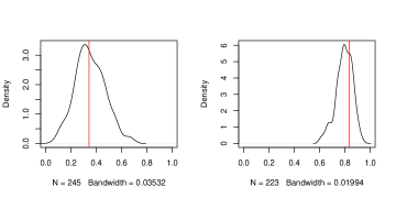
Figure 3.1: Angular density plots for $(\alpha,\gamma,\rho,\delta,n)=(0.3,0.7,0.2,2,50000)$ (left) and $(1,0,2,0.2,50000)$ (right). The red vertical lines are placed at $1/(1+a)$, with $a$ defined in (3.16).

We illustrate the full asymptotic dependence between in- and out-degrees by simulation. In Figure 3.1, we provide two empirical angular density plots for two sets of parameters: $(\alpha,\gamma,\rho,\delta,n)=(0.3,0.7,0.2,2,50000)$ (left) and $(1,0,0.2,2,50000)$ (right). The thresholds chosen in both cases are the 99.5%-percentile of $\{D^{\text{in}}_{w}(n)+D^{\text{out}}_{w}(n):1\leq w\leq n+1\}$. From Figure 3.1, we see that both angular density plots show a mode which is close to the red vertical lines placed at $1/(1+a)$, and $a$ is as specified in (3.16). Comparing the two panels in Figure 3.1, we observe that the $\alpha=1$ case shows less spread about the vertical line at $a/(1+a).$

3.3.2 Speculation on hidden regular variation.

When a limit measure concentrates on a subcone of the full state space, to improve estimates of probabilities in the complement of the subcone, we can seek a second hidden regular variation regime after removing the subcone. In the present case, $\mu(\cdot)$ concentrates on $\mathcal{L}_{a}$ and thus we may seek a regular variation property on $\mathbb{R}_{+}^{2}\setminus\mathcal{L}_{a}$ using a weaker scaling function $b_{0}(t)$ such that $t^{\lambda_{1}/(1+\rho+\delta)}/b_{0}(t)\to\infty$. See Das and Resnick (2017, 2015); Resnick (2007); Das et al. (2013); Lindskog et al. (2014). A convenient way to seek the hidden regular variation is by using generalized polar coordinates which in this case amount to the transformation

$$\boldsymbol{x}\to\Bigl{(}d_{2}(\boldsymbol{x},\mathcal{L}_{a}),\frac{\boldsymbol{x}}{d_{2}(\boldsymbol{x},\mathcal{L}_{a})}\Bigr{)},$$

where $d_{2}(\boldsymbol{x},\boldsymbol{y})$ is a metric on $\mathbb{R}_{+}^{2}\setminus\{\boldsymbol{0}\}$ chosen here for convenience to be the $L_{2}$-metric. The distance of a point $(x,y)$ to $\mathcal{L}_{a}$ is readily computed (Das and Resnick, 2017, p. 881) to be $d_{2}\bigl{(}(x,y),\mathcal{L}_{a}\bigr{)}={|y-ax|}/{\sqrt{1+a^{2}}},$ and we use a scaled version

$$d^{\prime}_{2}\bigl{(}(x,y),\mathcal{L}_{a}\bigr{)}=|y-ax|.$$ (3.22)

Hidden regular variation will be present for $(\mathcal{I},\mathcal{O})\stackrel{{\scriptstyle d}}{{=}}\widetilde{\boldsymbol{\xi}}_{\delta}(T^{*})$ if

$$tP\left[\left(\frac{d^{\prime}_{2}(\widetilde{\boldsymbol{\xi}}_{\delta}(T^{*}),\mathcal{L}_{a})}{b_{0}(t)},\frac{\widetilde{\boldsymbol{\xi}}_{\delta}(T^{*})}{d^{\prime}_{2}\left(\widetilde{\boldsymbol{\xi}}_{\delta}(T^{*}),\mathcal{L}_{a}\right)}\right)\in\cdot\,\right]$$

converges to a limit measure in $\mathbb{M}((0,\infty)\times\aleph_{\mathcal{L}_{a}})$ where $\aleph_{\mathcal{L}_{a}}=\{\boldsymbol{x}\in\mathbb{R}_{+}^{2}\setminus\mathcal{L}_{a}:d_{2}(\boldsymbol{x},\mathcal{L}_{a})=1\}$. Thus, considering (3.22), evidence consistent with this hidden regular variation is that

$$d^{\prime}_{2}(\widetilde{\boldsymbol{\xi}}_{\delta}(T^{*}),\mathcal{L}_{a})=\left|\widetilde{\xi}_{\delta}^{(2)}(T^{*})-a\widetilde{\xi}_{\delta}^{(1)}(T^{*})\right|$$

be a random variable with a regularly varying tail. Since $\widetilde{\boldsymbol{\xi}}_{\delta}(t)/e^{\lambda_{1}t}\stackrel{{\scriptstyle\text{a.s.}}}{{\longrightarrow}}\widetilde{L}\boldsymbol{v}$, we have

$$\frac{\xi_{\delta}^{(2)}(t)-a\xi_{\delta}^{(1)}(t)}{e^{\lambda_{1}t}}\stackrel{{\scriptstyle\text{a.s.}}}{{\longrightarrow}}\widetilde{L}v_{2}-a\widetilde{L}v_{1}=0,$$

so the index of the sought hidden regular variation needs to be smaller than the one indicated in (3.14). In what follows, we offer some (incomplete) evidence this is the case.

When $\delta=0$ and $\alpha<1$, $\widetilde{\boldsymbol{\xi}}_{0}(\cdot)$ becomes a two-type branching process without immigration. Then by (3.1), the second eigenvalue of $A$ is

$$\lambda_{2}=\frac{1}{2}(1-\sqrt{\Delta}),$$

and its associated right eigenvector is $\boldsymbol{u}^{\prime}=(a,-1)^{T}$. Note that Theorem 5 assumes $\lambda_{1}\geq\log 2$, i.e. $\sqrt{\Delta}\geq 2\log 2-1$, so that

$$\lambda_{1}-2\lambda_{2}=\frac{3}{2}\sqrt{\Delta}-\frac{1}{2}=3\log 2-2>0.$$

By (Athreya and Ney, 1972, Corollary V.8.1), one property for a 2-type branching process, $\widetilde{\boldsymbol{\xi}}_{0}(\cdot)$, is that if

$$\lambda_{1}>2\lambda_{2},$$ (3.23)

then there exists some normal random variable $V$ with mean 0 and some variance $\sigma^{2}>0$, such that

$$\lim_{t\to\infty} \mathbb{P}\left(0<x_{1}<\widetilde{L}\leq x_{2}<\infty,\,e^{-\lambda_{1}t/2}{\left|\widetilde{\xi}^{(2)}_{0}(t)-a\widetilde{\xi}^{(1)}_{0}(t)\right|}\leq y\right)$$

$$=\int_{x_{1}}^{x_{2}}f_{\widetilde{L}}(z)\mathbb{P}\left(|V|\leq\frac{y}{\sqrt{z}}\right)\mathrm{d}z.$$ (3.24)

In (3.24), the distribution of $\widetilde{L}$ as well as the constant $\sigma$ depend on ${\widetilde{\boldsymbol{\xi}}_{0}(0)}$, but for brevity of notation, we suppress the conditioning on ${\widetilde{\boldsymbol{\xi}}_{0}(0)}$. Based on (3.24), we make the following conjecture: if it were true that for $q^{\prime}>2(1+\rho)/\lambda_{1}$,

$$\sup_{t\geq 0}e^{-\lambda_{1}q^{\prime}t/2}\mathbb{E}\left(\left|\widetilde{\xi}^{(2)}_{0}(t)-a\widetilde{\xi}^{(1)}_{0}(t)\right|^{q^{\prime}}\right)<\infty,$$ (3.25)

then

$$t\mathbb{P}\Bigl{(} \frac{\left|\mathcal{O}-a\mathcal{I}\right|}{t^{\lambda_{1}/(2(1+\rho))}}>y\Bigr{)}=t\mathbb{P}\left(\frac{\left|\widetilde{\xi}^{(2)}_{0}(T^{*})-a\widetilde{\xi}^{(1)}_{0}(T^{*})\right|}{t^{\lambda_{1}/(2(1+\rho))}}>y\right)$$

$$\longrightarrow\frac{1+\rho}{\lambda_{1}}\int_{0}^{\infty}u^{-1-(1+\rho)/\lambda_{1}}\int_{0}^{\infty}f_{\widetilde{L}}(z)\mathbb{P}\left(|V|>\frac{y}{\sqrt{uz}}\right)\mathrm{d}z,\qquad{(t\to\infty)}.$$ (3.26)

We have not been able to prove the moment condition (3.25). However, we offer simulation evidence for (3.3.2) and simulate a network with parameters

$$(\alpha,\gamma,\rho,\delta,n)=(0.2,0.8,0.25,{0},50000),$$

so that $\lambda_{1}=0.816>\log 2$, and $\lambda_{2}=0.184<\lambda_{1}/2$.

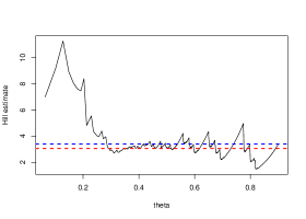
Figure 3.2: AltHill plot based on (3.27) with $(\alpha,\gamma,\rho,\delta,n)=(0.2,0.8,0.25,0,50000)$. The red and blue lines represent the true and estimated values of $2(1+\rho)/\lambda_{1}$, respectively.

In Figure 3.2, we present the altHill plot (cf. Drees et al. (2000)) based on

$$\left\{\left|aD^{\text{in}}_{w}(n)-D^{\text{out}}_{w}(n)\right|:w\in V(n)\right\}.$$ (3.27)

The red dashed line is the true value of $2(1+\rho)/\lambda_{1}$, and the blue line corresponds to the estimated value of $2(1+\rho)/\lambda_{1}$ using the minimum distance method in Clauset et al. (2009). The altHill plot supports our conjecture in (3.3.2). For $\delta>0$, we have similar speculation as in (3.3.2), i.e. we conjecture $\left|\mathcal{O}-a\mathcal{I}\right|$ be regularly varying with index $2(1+\rho+\delta)/\lambda_{1}$. We repeat the simulation procedure above for a different set of parameters:

$$(\alpha,\gamma,\rho,\delta,n)=(0.2,0.8,0.25,0.5,50000).$$

The corresponding altHill plot is given in Figure 3.3. The red dashed line is the true value of $2(1+\rho+\delta)/\lambda_{1}$, and the blue line corresponds to the estimated value of $2(1+\rho+\delta)/\lambda_{1}$. These provide evidence for our conjecture, even when $\delta=0.5>0$.

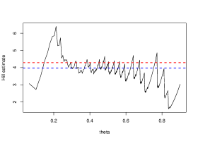
Figure 3.3: AltHill plot based on (3.27) with $(\alpha,\gamma,\rho,\delta,n)=(0.2,0.8,0.25,0.5,50000)$. The red and blue lines represent the true and estimated values of $2(1+\rho+\delta)/\lambda_{1}$, respectively.

4 Potential Extensions of the Model

Now that we have studied theoretical properties of the proposed PA model with reciprocity, this section discusses possible extensions that we will investigate in the future.

Randomized $\rho$.

So far we have assumed that each node has a common and fixed reciprocity parameter, $\rho\in(0,1)$ but this may not reflect realistic behavior and allow good fits to datasets. For instance, users on Facebook (nodes) may have their own probabilities to respond to a post on his/her wall. Keeping such heterogeneity in mind, we consider a randomized scenario: for each node $v\geq 1$, upon its creation, its affiliated reciprocity probability, $U_{v}$, is uniformly distributed on $[A,B]$. Here we also assume $0\leq A\leq B\leq 1$, and $\{U_{v}:v\geq 1\}$ are iid.

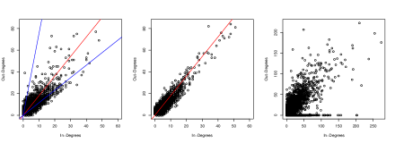
Figure 4.1: Scatter plots of simulated in- and out-degrees from PA models with randomized (left) and fixed (middle) reciprocity, as well as those from Facebook wall posts between 2006-01-01 and 2007-02-25. We set $(\alpha,\gamma,\delta,n)=(0.2,0.8,0.5,10^{5})$. The random reciprocity is uniform on $[0.1,0.8]$ and the fixed reciprocity $\rho=0.45$. Red lines in left and middle panels correspond to $\mathcal{L}_{a}=\{(x,y)\in\mathbb{R}^{2}_{+}:y=1.805x\}$, and the two blue lines in the left panel constructs $[\text{wedge}]$ as in (4.1).

We use simulation to inspect features of this PA model with randomized reciprocity. Set $(\alpha,\gamma,\delta,n)=(0.2,0.8,0.5,10^{5})$, and simulate a PA network with randomized reciprocity using $(A,B)=(0.1,0.8)$, and the scatter plot of simulated out- vs in-degrees is presented in the left panel of Figure 4.1. Since in this case $\mathbb{E}(U_{1})=0.45$, for comparison purposes, we also include a scatter plot from a PA network with fixed reciprocity, i.e. $(\alpha,\gamma,\rho,\delta,n)=(0.2,0.8,0.45,0.5,10^{5})$, in the middle panel of Figure 4.1. When $\rho=0.45$, the slope of $\mathcal{L}_{a}$, is calculated from (3.16), i.e. $a=1.805$, and $\mathcal{L}_{a}$ is marked as the red line in left and middle panels of Figure 4.1. In the right panel of Figure 4.1, we also include the scatter plot of out- vs in-degrees from the Facebook wall posts data (available at http://konect.cc/networks/facebook-wosn-wall/) between 2006-01-01 and 2007-02-25.

The three panels in Figure 4.1 show that a randomized reciprocity parameter tends to generate a scatter plot which matches the real data example better. In addition, based on the left and middle scatter plots, we see that in- and out-degrees from the model with randomized reciprocity are less concentrating around $\mathcal{L}_{a}$. The two blue lines in the left panel of Figure 4.1 correspond to the concentration lines for $\rho=A,B$, whose slopes are equal to 7.533 and 2, respectively. The left panel of Figure 4.1 shows that large in- and out-degrees are concentrating within the wedge:

$$[\text{wedge}]:=\{(x,y)\in\mathbb{R}^{2}_{+}:1.154x\leq y\leq 7.533x\}.$$ (4.1)

This phenomenon coincides with the notion of strong asymptotic dependence as discussed in Das and Resnick (2017), and has been detected in real datasets(cf. (Das and Resnick, 2017, Section 5)), but the rigorous justification under the network setup needs working out.

Adding edges between existing nodes.

The model proposed in Section 1.1 requires adding a new node at each step, and the offset parameters are identical for the evolution of both in- and out-degrees. These assumptions are restrictive in practice. We create an extended model by including the following scenario added to cases (i) and (ii) in Section 1.1:

1. With probability $\beta\in(0,1)$, we add an edge $(w_{1},w_{2})$ between two existing nodes $w_{1},w_{2}\in V(n)$, with probability

   $$\frac{D^{\text{in}}_{w_{2}}(n)+\delta}{\sum_{w_{2}\in V(n)}(D^{\text{in}}_{w_{2}}(n)+\delta)}\frac{D^{\text{out}}_{w_{1}}(n)+\delta}{\sum_{w_{1}\in V(n)}(D^{\text{out}}_{w_{1}}(n)+\delta)}$$

   $$=\frac{D^{\text{in}}_{w_{2}}(n)+\delta}{|E(n)|+\delta_{\text{in}}|V(n)|}\frac{D^{\text{out}}_{w_{1}}(n)+\delta}{|E(n)|+\delta|V(n)|}.$$

   Then with probability $\rho\in(0,1)$, we add a reciprocal edge $(w_{2},w_{1})$. We then update the edge set as $E(n+1)=E(n)\cup\{(w_{1},w_{2}),(w_{2},w_{1})\}$. If the reciprocal edge is not created, then $E(n+1)=E(n)\cup\{(w_{1},w_{2})\}$.

With this third scenario, both the number of nodes and of edges in $G(n)$ are random. The $\beta$-scenario makes the model more realistic since a large proportion of edges are created between two existing nodes in real datasets (e.g. those listed on KONECT Kunegis (2013)). However, the additional scenario does not fit into the embedding framework directly, as it may simultaneously increase the in- and out-degrees of two different nodes. In addition, the HRV conjecture in Section 3.3.2 is based on the condition that $\lambda_{1}>2\lambda_{2}$, which is a direct result from the $\lambda_{1}\geq\log 2$ assumption in Theorem 5. With the additional $\beta$-scenario, it is possible to have $\lambda_{1}<2\lambda_{2}$, which may lead to different limiting behavior of $d^{\prime}_{2}((\mathcal{I},\mathcal{O}),\mathcal{L}_{a})$.

Asymptotic dependence in higher dimensions.

Another possible extension is to consider the multitype branching structure with $K\geq 2$. For instance, when modeling the retweet or reply network on Twitter, the follower/following relationship may also have an impact on the generation of retweets or replies (directed edges). Assume each node (user) to have four different degrees: ordinary in- and out-degrees, together with the numbers of followers and accounts one is following. Then an embedding framework using four-type branching processes may provide a resolution to uncover the asymptotic dependence structure between retweeting degrees and friendship degrees.

We will explore further in all these directions in our future research.

5 Proofs

5.1 Proof of Theorem 1

By (Athreya and Ney, 1972, Theorem V.8.1), we see that

$$\left\{e^{-\lambda_{t}}\boldsymbol{u}\cdot\boldsymbol{\Psi}_{k}(t):t\geq 0\right\}$$

is a martingale with respect to the filtration $\sigma\left(\boldsymbol{\Psi}_{k}(s):0\leq s\leq t\right)$. Also, discussion in Chapter V.7.4 of Athreya and Ney (1972) shows that for $k\geq 0$,

$$\sup_{t\geq 0}\mathbb{E}\left[\left(e^{-\lambda_{1}t}\boldsymbol{u}\cdot\boldsymbol{\Psi}_{k}(t)\right)^{2}\right]<\infty.$$

Therefore, $\{e^{-\lambda_{1}t}\boldsymbol{u}\cdot\boldsymbol{\xi}_{\theta}(t):t\geq 0\}$ is a non-negative sub-martingale with respect to $\sigma\left(\boldsymbol{\xi}_{\theta}(s):0\leq s\leq t\right)$, and

$$\sup_{t\geq 0} \mathbb{E}\left(e^{-\lambda_{1}t}\boldsymbol{u}\cdot\boldsymbol{\xi}_{\theta}(t)\right)=\sup_{t\geq 0}\sum_{k=0}^{\infty}\mathbb{E}\left(e^{-\lambda_{1}\tau_{k}}e^{-\lambda_{1}(t-\tau_{k})}\boldsymbol{u}\cdot\boldsymbol{\Psi}_{k}(t-\tau_{k})\boldsymbol{1}_{\{t\geq\tau_{k}\}}\right)$$

$$\leq\sum_{k=0}^{\infty}\left(\mathbb{E}\left(e^{-2\lambda_{1}\tau_{k}}\right)\right)^{1/2}\sup_{t\geq 0}\left(\mathbb{E}\left[\left(e^{-\lambda_{1}t}\boldsymbol{u}\cdot\boldsymbol{\Psi}_{0}(t)\right)^{2}\right]\right)^{1/2}<\infty.$$

Then we conclude that there exists some random variable $I_{0}$ such that as $t\to\infty$,

$$e^{-\lambda_{1}t}\boldsymbol{u}\cdot\boldsymbol{\xi}_{\theta}(t)\stackrel{{\scriptstyle\text{a.s.}}}{{\longrightarrow}}I_{0}.$$

Also, since

$$\left(e^{-\lambda_{1}t}\boldsymbol{u}\cdot\boldsymbol{\xi}_{\theta}(t)\right)^{2}$$

$$= \left(\sum_{k=0}^{\infty}e^{-\lambda_{1}\tau_{k}}e^{-\lambda_{1}(t-\tau_{k})}\boldsymbol{u}\cdot\boldsymbol{\Psi}_{k}(t-\tau_{k})\boldsymbol{1}_{\{t\geq\tau_{k}\}}\right)^{2}$$

$$\leq \left(\sum_{k=0}^{\infty}e^{-\lambda_{1}\tau_{k}}\right)\left(\sum_{k=0}^{\infty}e^{-\lambda_{1}\tau_{k}}\left(e^{-\lambda_{1}(t-\tau_{k})}\boldsymbol{u}\cdot\boldsymbol{\Psi}_{k}(t-\tau_{k})\boldsymbol{1}_{\{t\geq\tau_{k}\}}\right)^{2}\right),$$

then

$$\mathbb{E}\left[\left(e^{-\lambda_{1}t}\boldsymbol{u}\cdot\boldsymbol{\xi}_{\theta}(t)\right)^{2}\right]$$

$$\leq \sup_{t\geq 0}\mathbb{E}\left[\left(e^{-\lambda_{1}t}\boldsymbol{u}\cdot\boldsymbol{\Psi}_{0}(t)\right)^{2}\right]\mathbb{E}\left[\sum_{k=0}^{\infty}e^{-\lambda_{1}\tau_{k}}\left(\sum_{k=0}^{\infty}e^{-\lambda_{1}\tau_{k}}\right)\right]$$

$$\leq \sup_{t\geq 0}\mathbb{E}\left[\left(e^{-\lambda_{1}t}\boldsymbol{u}\cdot\boldsymbol{\Psi}_{0}(t)\right)^{2}\right]\sum_{k=0}^{\infty}\left(\mathbb{E}\left(e^{-2\lambda_{1}\tau_{k}}\right)\right)^{1/2}\left(\mathbb{E}\left[\left(\sum_{k=0}^{\infty}e^{-\lambda_{1}\tau_{k}}\right)^{2}\right]\right)^{1/2}$$

$$< \infty.$$

Hence, we have

$$\mathbb{E}\left(I_{0}\right) =\lim_{t\to\infty}\mathbb{E}\left(e^{-\lambda_{1}t}\boldsymbol{u}\cdot\boldsymbol{\xi}_{\theta}(t)\right)$$

$$=\lim_{t\to\infty}\sum_{k=0}^{\infty}\mathbb{E}\left(e^{-\lambda_{1}\tau_{k}}\right)\mathbb{E}\left(e^{-\lambda_{1}(t-\tau_{k})}\boldsymbol{u}\cdot\boldsymbol{\Psi}_{k}(t-\tau_{k})\boldsymbol{1}_{\{t\geq\tau_{k}\}}\right)$$

$$=\sum_{k=0}^{\infty}\mathbb{E}\left(e^{-\lambda_{1}\tau_{k}}\right)\mathbb{E}\left(W_{k}\right)=\mathbb{E}\left(\sum_{k=0}^{\infty}e^{-\lambda_{1}\tau_{k}}W_{k}\right).$$

In addition, by Fatou’s lemma, we see that a.s.

$$I_{0}\geq\sum_{k=0}^{\infty}e^{-\lambda_{1}\tau_{k}}W_{k}.$$

Then we conclude that

$$I_{0}=\sum_{k=0}^{\infty}e^{-\lambda_{1}\tau_{k}}W_{k}\qquad\text{a.s.}.$$

Then for $i=1,\ldots,K$, we see that

$$e^{-\lambda_{1}t}\xi_{\theta}^{(i)}(t) =e^{-\lambda_{1}t}\sum_{k=0}^{\infty}\frac{\psi_{k}^{(i)}(t-\tau_{k})}{\boldsymbol{u}\cdot\boldsymbol{\Psi}_{k}(t-\tau_{k})}\boldsymbol{u}\cdot\boldsymbol{\Psi}_{k}(t-\tau_{k})\boldsymbol{1}_{\{t\geq\tau_{k}\}}.$$

For fixed $M>0$, it follows from (2.2) that

$$e^{-\lambda_{1}t}\sum_{k=0}^{M}\frac{\psi_{k}^{(i)}(t-\tau_{k})}{\boldsymbol{u}\cdot\boldsymbol{\Psi}_{k}(t-\tau_{k})}\boldsymbol{u}\cdot\boldsymbol{\Psi}_{k}(t-\tau_{k})\boldsymbol{1}_{\{t\geq\tau_{k}\}}\stackrel{{\scriptstyle\text{a.s.}}}{{\longrightarrow}}\sum_{k=0}^{M}e^{-\lambda_{1}\tau_{k}}W_{k}v_{i}.$$

Also, since all entries of $\boldsymbol{u}$ are strictly positive, we then have

$$\lim_{M\to\infty}\lim_{t\to\infty} e^{-\lambda_{1}t}\sum_{k=M+1}^{\infty}\left|\frac{\psi_{k}^{(i)}(t-\tau_{k})}{\boldsymbol{u}\cdot\boldsymbol{\Psi}_{k}(t-\tau_{k})}-v_{i}\right|\boldsymbol{u}\cdot\boldsymbol{\Psi}_{k}(t-\tau_{k})\boldsymbol{1}_{\{t\geq\tau_{k}\}}$$

$$\leq\left(\frac{1}{u_{i}}+v_{i}\right)\lim_{M\to\infty}\lim_{t\to\infty}\sum_{k=M+1}^{\infty}e^{-\lambda_{1}t}\boldsymbol{u}\cdot\boldsymbol{\Psi}_{k}(t-\tau_{k})\boldsymbol{1}_{\{t\geq\tau_{k}\}}\stackrel{{\scriptstyle a.s.}}{{=}}0,$$

which completes the proof of the theorem.

5.2 Proof of Theorem 3

To show (i) in $\mathbb{M}\left(\mathbb{R}_{+}^{p}\times(\mathbb{R}_{+}\setminus\{0\})\right)$, take $f\in\mathcal{C}\bigl{(}\mathbb{R}_{+}^{2}\times(\mathbb{R}_{+}\setminus\{0\})\bigr{)}$, which is bounded, uniformly continuous, and satisfies that for some $\varepsilon_{0}>0$, $f(\boldsymbol{x},y)=0$ if $y<\varepsilon_{0}$. Then to prove (2.18), we show

$$\lim_{t\to\infty} t\mathbb{E}\left[f\left({{\boldsymbol{\xi}}(X)},\frac{X}{b(t)}\right)\right]=\int_{\varepsilon_{0}}^{\infty}\mathbb{E}\left[f\bigl{(}\boldsymbol{\xi}_{\infty},y\bigr{)}\right]\nu_{c}(\mathrm{d}y).$$ (5.1)

Rewrite the left hand side of (5.1) as

$$t\mathbb{E}\left[f\left({\boldsymbol{\xi}(X)},\frac{X}{b(t)}\right)\right]-t\mathbb{E}\left[f\left(\boldsymbol{\xi}_{\infty},\frac{X}{b(t)}\right)\right]$$

$$\quad+t\mathbb{E}\left[f\left(\boldsymbol{\xi}_{\infty},\frac{X}{b(t)}\right)\right]-\int_{\varepsilon_{0}}^{\infty}\mathbb{E}\left[f\bigl{(}\boldsymbol{\xi}_{\infty},y\bigr{)}\right]\nu_{c}(\mathrm{d}y)$$

$$\quad+\int_{\varepsilon_{0}}^{\infty}\mathbb{E}\left[f\bigl{(}\boldsymbol{\xi}_{\infty},y\bigr{)}\right]\nu_{c}(\mathrm{d}y)$$

$$=:I_{t}+II_{t}+\int_{\varepsilon_{0}}^{\infty}\mathbb{E}\left[f\bigl{(}\boldsymbol{\xi}_{\infty},y\bigr{)}\right]\nu_{c}(\mathrm{d}y),$$

and we will show that both $|I_{t}|$ and $|II_{t}|$ go to 0 as $t\to\infty$.

For $II_{t}$, we see that

$$t \mathbb{E}\left[f\left(\boldsymbol{\xi}_{\infty},\frac{X}{b(t)}\right)\right]=\int_{\varepsilon_{0}}^{\infty}f\left(\boldsymbol{x},y\right)\mathbb{P}\left(\boldsymbol{\xi}_{\infty}\in\mathrm{d}\boldsymbol{x}\right)\times t\mathbb{P}\left(\frac{X}{b(t)}\in\mathrm{d}y\right).$$

For any fixed $\boldsymbol{x}\in\mathbb{R}_{+}^{2}$, $f(\boldsymbol{x},\cdot)\in\mathcal{C}(\mathbb{R}_{+}\setminus\{0\})$ so that as $t\to\infty$,

$$\int_{\varepsilon_{0}}^{\infty}f(\boldsymbol{x},y)\times t\mathbb{P}\left(\frac{X}{b(t)}\in\mathrm{d}y\right)\longrightarrow\int_{\varepsilon_{0}}^{\infty}f(\boldsymbol{x},y)\nu_{c}(\mathrm{d}y).$$

Since $f$ is bounded, there exists some constant $K_{0}>0$ such that

$$\sup_{\boldsymbol{x}\in\mathbb{R}_{+}^{2},y\geq\varepsilon_{0}}f(\boldsymbol{x},y)\leq K_{0},$$

and for all $t$,

$$\sup_{\boldsymbol{x}\in\mathbb{R}_{+}^{2},y\geq\varepsilon_{0}} \int_{\varepsilon_{0}}^{\infty}f(\boldsymbol{x},y)\times t\mathbb{P}\left(\frac{X}{b(t)}\in\mathrm{d}y\right)$$

$$\leq K_{0}\times t\mathbb{P}\left(\frac{X}{b(t)}>\varepsilon_{0}\right)\longrightarrow K_{0}\varepsilon_{0}^{-c}<\infty.$$

Then by dominated convergence, we see that $|II_{t}|\to 0$, as $t\to\infty$.

Now we consider the first term $I_{t}$. Since $\boldsymbol{\xi}(t)\to\boldsymbol{\xi}_{\infty}$ almost surely, by Egorov’s Theorem, for any $\varepsilon>0$, there exists an $\omega$-set $A_{\varepsilon}$ such that

$$\sup_{\omega\in A_{\varepsilon}}\left|{\boldsymbol{\xi}}(t,\omega)-\boldsymbol{\xi}_{\infty}(\omega)\right|\longrightarrow 0,$$

and $\mathbb{P}(A_{\varepsilon}^{c})<\varepsilon$. Then we bound $|I_{t}|$ by

$$|I_{t}| \leq\mathbb{E}\left[\left|f\left({\boldsymbol{\xi}(X)},\frac{X}{b(t)}\right)-f\left(\boldsymbol{\xi}_{\infty},\frac{X}{b(t)}\right)\right|\boldsymbol{1}_{A_{\varepsilon}\cap\{{X}/{b(t)}\geq\varepsilon_{0}\}}\right]$$

$$\quad+\mathbb{E}\left[\left|f\left({\boldsymbol{\xi}(X)},\frac{X}{b(t)}\right)-f\left(\boldsymbol{\xi}_{\infty},\frac{X}{b(t)}\right)\right|\boldsymbol{1}_{A^{c}_{\varepsilon}\cap X/b(t)\geq\varepsilon_{0}\}}\right]$$

$$=:I^{a}_{t}+I^{b}_{t}.$$ (5.2)

Let $d\left((\boldsymbol{x},y),(\boldsymbol{x}^{\prime},y^{\prime})\right)$ denote the distance between $(\boldsymbol{x},y)$ and $(\boldsymbol{x}^{\prime},y^{\prime})$ on $\mathbb{R}_{+}^{p}\times\mathbb{R}_{+}\setminus\{0\}$ and recall the modulus of continuity of $f$ given in (2.15). Applying Egorov’s Theorem, for a given $\eta>0$, there exists $M_{0}>0$ such that

$$\sup_{t\geq M_{0}}\sup_{\omega\in A_{\varepsilon}}\left|{\boldsymbol{\xi}}(t,\omega)-\boldsymbol{\xi}_{\infty}(\omega)\right|\leq\eta.$$

Then as long as $t$ is large enough such that $b(t)\varepsilon_{0}>M_{0}$, we have

$$I^{a}_{t} \leq\Delta_{f}\left(\eta\right)t\mathbb{P}\left(A_{\varepsilon}\cap\left\{\frac{X}{b(t)}\geq\varepsilon_{0}\right\}\right)$$

$$\leq\Delta_{f}\left(\eta\right)t\mathbb{P}\left(\frac{X}{b(t)}\geq\varepsilon_{0}\right)\stackrel{{\scriptstyle t\to\infty}}{{\longrightarrow}}\Delta_{f}\left(\eta\right)\varepsilon_{0}^{-c}\stackrel{{\scriptstyle\eta\to 0}}{{\longrightarrow}}0.$$

For $I^{b}_{t}$, we have

$$I^{b}_{t} \leq 2K_{0}\times t\mathbb{P}\left(A_{\varepsilon}^{c}\cap\left\{\frac{X}{b(t)}\geq\varepsilon_{0}\right\}\right),$$

and since $$A^{c}_{\varepsilon}\in\sigma\{{\boldsymbol{\xi}}(t):t\geq 0\} X \{{\boldsymbol{\xi}}(t):t\geq 0\}$$, and is independent of , then

$$=2K_{0}\mathbb{P}\left(A_{\varepsilon}^{c}\right)t\mathbb{P}\left(\frac{X}{b(t)}\geq\varepsilon_{0}\right)$$

$$\stackrel{{\scriptstyle t\to\infty}}{{\longrightarrow}}2K_{0}\mathbb{P}\left(A_{\varepsilon}^{c}\right)\varepsilon_{0}^{-c}\leq 2K_{0}\varepsilon\cdot\varepsilon_{0}^{-c}.$$

So $|I_{t}|\to 0$, as $t\to\infty$, which completes the proof of (2.18).

Now we turn to the proof of (2.20) in part (ii). Define a mapping $\chi:\mathbb{R}_{+}^{2}\times(\mathbb{R}_{+}\setminus\{0\})\mapsto\mathbb{R}_{+}^{2}\times(\mathbb{R}_{+}\setminus\{0\})$ by $\chi((x,y),\sigma)=\bigl{(}(\sigma x,\sigma y),\sigma\bigr{)}.$ Then by (Lindskog et al., 2014, Example 3.3), we apply $\chi$ to the convergence in (2.18) to obtain that in $\mathbb{M}\left(\mathbb{R}_{+}^{2}\times(\mathbb{R}_{+}\setminus\{0\})\right)$,

$$t\mathbb{P}\left[\left(\frac{\boldsymbol{\xi}(X)X}{b(t)},\frac{X}{b(t)}\right)\in\cdot\right]\to\left(\mathbb{P}\left[\boldsymbol{\xi}_{\infty}\in\cdot\right]\times\nu_{c}\right)\circ\chi^{-1}(\cdot).$$ (5.3)

Let $g\in\mathcal{C}(\mathbb{R}_{+}^{2}\setminus\{\boldsymbol{0}\})$, and $g(\boldsymbol{x})=0$ if $\|\boldsymbol{x}\|\leq\theta$ for some $\theta>0$ with $\sup_{\boldsymbol{x}}|g(\boldsymbol{x})|=:\|g\|.$ For typographical simplicity, assume $\|g\|=1.$ We can prove (2.20) by showing

$$t\mathbb{E}g\Bigl{(}\frac{\boldsymbol{\xi}(X)X}{b(t)}\Bigr{)}\to\int_{0}^{\infty}\mathbb{E}g(\boldsymbol{\xi}_{\infty}x)\nu_{c}(dx),$$ (5.4)

knowing that from (5.3), for any $\eta>0$,

$$t\mathbb{E} \left[g\Bigl{(}\frac{\boldsymbol{\xi}(X)X}{b(t)}\Bigr{)}1_{[X/b(t)>\eta]}\right]$$

$$\to\int_{\eta}^{\infty}\mathbb{E}g\bigl{(}h(\boldsymbol{\xi}_{\infty},x)\bigr{)}\nu_{c}(dx)=\int_{\eta}^{\infty}\mathbb{E}g(\boldsymbol{\xi}_{\infty}x)\nu_{c}(dx).$$ (5.5)

Differencing the left sides of (5.4) and (5.2) we must show

$$\lim_{\eta\to 0}\limsup_{t\to\infty}t\mathbb{E}\left[g\Bigl{(}\frac{\boldsymbol{\xi}(X)X}{b(t)}\Bigr{)}\boldsymbol{1}_{\{X/b(t)\leq\eta\}}\right]=0.$$ (5.6)

Bearing in mind the support of $g$, we have

$$t\mathbb{E}\left[g\Bigl{(}\frac{\boldsymbol{\xi}(X)X}{b(t)}\Bigr{)}\boldsymbol{1}_{\{X/b(t)\leq\eta\}}\right]\leq t\mathbb{P}\Bigl{(}\left\|\frac{\boldsymbol{\xi}(X)X}{b(t)}\right\|>\theta,\frac{X}{b(t)}\leq\eta\Bigr{)}$$

$$=t\mathbb{P}\Bigl{(}\left\|\frac{\boldsymbol{\xi}(X)X}{b(t)}\boldsymbol{1}_{\{X/b(t)\leq\eta\}}\right\|>\theta\Bigr{)}$$

$$\leq \theta^{-c^{\prime}}t\mathbb{E}\left\|\frac{\boldsymbol{\xi}(X)X}{b(t)}\boldsymbol{1}_{\{X/b(t)\leq\eta\}}\right\|^{c^{\prime}}$$

and recalling $$\boldsymbol{\xi}(\cdot) X$$ and are independent, this is evaluated to

$$= \theta^{-c^{\prime}}\int_{0}^{\eta}\mathbb{E}\left\|{\boldsymbol{\xi}(b(t)s)}\right\|^{c^{\prime}}s^{c^{\prime}}tP(X/b(t)\in ds)$$

$$\leq \theta^{-c^{\prime}}\kappa t\mathbb{E}\left[\left(\frac{X}{b(t)}\right)^{c^{\prime}}\boldsymbol{1}_{\{X/b(t)\leq\eta\}}\right]$$

and applying Karamata’s theorem on integration, this converges as $$t\to\infty$$

$$= \theta^{-c^{\prime}}\kappa\eta^{c^{\prime}-c}\to 0,$$

as $\eta\to 0$ giving (5.6) and hence (5.4).

5.3 Proof of Equation (3.17)

We will now prove the claim in (3.17) by showing a bound of the moment of a $K$-type branching process with immigration. We start with analyzing the $q$-th moment of a $K$-type branching process as given in Section 2.1.1, for $q\geq 2$. Then with the construction of a $K$-type branching process with immigration as in (2.3), we derive the bound of its $q$-th moment.

Proposition 1

Let $\{\boldsymbol{\Psi}_{0}(t):t\geq 0\}$ be a continuous time $K$-type branching process with matrix $A$ as given in (2.1), and $\boldsymbol{u}$ be the right eigenvector associated with the largest eigenvalue of $A$, i.e. $\lambda_{1}$. Suppose that $Y_{j}^{(i)}$ is the number of type $j$ particles produced by a type $i$ particle at the end of its lifetime, and

$$Y_{j}^{(i)}\leq e^{\lambda_{1}},\qquad\text{for all }\quad i,j=1,\ldots,K.$$ (5.7)

Then for an integer $q\geq 1$, we have

$$\sup_{t\geq 0}e^{-\lambda_{1}qt}\mathbb{E}\left[\left(\boldsymbol{u}\cdot\boldsymbol{\Psi}_{0}(t)\right)^{q}\right]<\infty.$$ (5.8)

Proof

Note that for $n\geq 0$ integer, $\{\boldsymbol{\Psi}_{0}(n):n\geq 0\}$ is a discrete time $K$-type branching process, and we have

$$\sup_{t\geq 0}e^{-\lambda_{1}qt}\mathbb{E}\left[\left(\boldsymbol{u}\cdot\boldsymbol{\Psi}_{0}(t)\right)^{q}\right]\leq e^{\lambda_{1}}\sup_{n\geq 0}e^{-\lambda_{1}qn}\mathbb{E}\left[\left(\boldsymbol{u}\cdot\boldsymbol{\Psi}_{0}(n)\right)^{q}\right].$$

Hence it suffices to show for some constant $C^{\prime}_{q}>0$,

$$\sup_{n\geq 0}e^{-\lambda_{1}qn}\mathbb{E}\left[\left(\boldsymbol{u}\cdot\boldsymbol{\Psi}_{0}(n)\right)^{q}\right]\leq C^{\prime}_{q}.$$ (5.9)

The proof of (5.9) for $q=1,2$ has been given in (Athreya and Ney, 1972, Chapter V.7.4). Here we use induction to show (5.9) also holds for $q\geq 3$. Suppose (5.9) is true for $k=1,\ldots,q$, $q\geq 2$, and define

$$Z_{n}:=e^{-\lambda_{1}n}\left(\boldsymbol{u}\cdot\boldsymbol{\Psi}_{0}(n)\right).$$

We need to prove that for some $C^{\prime}_{q+1}>0$,

$$\sup_{n\geq 0}\mathbb{E}\left[\left(Z_{n}\right)^{q+1}\right]\leq C^{\prime}_{q+1}.$$ (5.10)

Note also that by (Athreya and Ney, 1972, Theorem V.8.1), $Z_{n}$ is a martingale with respect to the filtration $\mathcal{F}^{\prime}_{n}:=\sigma\{Z_{k}:k\leq n\}$ for $n\geq 0$. Also, under $\mathbb{P}^{\mathcal{F}^{\prime}_{n}}$,

$$Z_{n+1}\stackrel{{\scriptstyle d}}{{=}}e^{-\lambda_{1}(n+1)}\sum_{j=1}^{K}u_{j}\sum_{i=1}^{K}\sum_{l=1}^{\psi_{0}^{(i)}(n)}Y^{(i)}_{j,l},$$ (5.11)

then we see from (5.11) that for $q\geq 2$,

$$\mathbb{E}^{\mathcal{F}^{\prime}_{n}}\left(Z_{n+1}^{q}\right) \leq e^{-\lambda_{1}(n+1)q}\left(e^{\lambda_{1}}\boldsymbol{u}\cdot\boldsymbol{\Psi}_{0}(n)\right)^{q}=Z_{n}^{q}.$$ (5.12)

Next, we apply Lemma 2.1 in Athreya et al. (2008) to obtain that

$$\mathbb{E}^{\mathcal{F}^{\prime}_{n}}\left(Z_{n+1}^{q+1}\right)\leq\mathbb{E}^{\mathcal{F}^{\prime}_{n}}\left(Z_{n+1}^{q}\right)\mathbb{E}^{\mathcal{F}^{\prime}_{n}}\left(Z_{n+1}\right)$$

$$\,+\sum_{k=1}^{q}{q\choose k}\mathbb{E}^{\mathcal{F}^{\prime}_{n}}\left(Z_{n+1}^{q-k}\right)e^{-\lambda_{1}(k+1)(n+1)}\sum_{j=1}^{K}u_{j}\sum_{i=1}^{K}\sum_{l=1}^{\psi_{0}^{(i)}(n)}\mathbb{E}^{\mathcal{F}^{\prime}_{n}}\left[\left(Y^{(i)}_{j,l}\right)^{k+1}\right],$$

which by (5.12) is bounded by

$$\leq Z_{n}^{q+1}+\sum_{k=1}^{q}{q\choose k}Z_{n}^{q-k}e^{-\lambda_{1}(k+1)(n+1)}e^{\lambda_{1}(k+1)}\left(\boldsymbol{u}\cdot\boldsymbol{\Psi}_{0}(n)\right)$$

$$=Z_{n}^{q+1}+\sum_{k=1}^{q}{q\choose k}Z_{n}^{q-k+1}e^{-\lambda_{1}(k+1)(n+1)+\lambda_{1}n}e^{\lambda_{1}(k+1)}$$

$$=Z_{n}^{q+1}+\sum_{k=1}^{q}{q\choose k}Z_{n}^{q-k+1}e^{-\lambda_{1}kn}.$$

Then we have

$$\sup_{n\geq 0}\mathbb{E}\left(Z_{n}^{q+1}\right) \leq\mathbb{E}\left(Z_{0}^{q+1}\right)+\sum_{k=1}^{q}{q\choose k}\sum_{n=0}^{\infty}e^{-\lambda_{1}kn}\mathbb{E}\left(Z_{n}^{q-k+1}\right).$$ (5.13)

By the induction hypothesis, we have that $\sup_{n\geq 0}\mathbb{E}\left(Z_{n}^{q-k+1}\right)\leq C^{\prime}_{q-k+1}$, $k=1,\ldots,q$. In addition, $\sum_{n\geq 0}e^{-\lambda_{1}kn}<\infty$, then (5.10) follows directly from (5.13).

Using the distribution representation in (2.3), we now give the moment bound for a $K$-type branching process with immigration.

Proposition 2

Denote the $K$-type branching process with immigration given in (2.3) as

$$\left\{\boldsymbol{\xi}_{\theta}(t)\equiv(\xi^{(1)}_{\theta}(t),\ldots,\xi^{(K)}_{\theta}(t)):t\geq 0\right\}.$$

Suppose that the condition in (5.7) holds, then we have

$$\sup_{t\geq 0}e^{-\lambda_{1}qt}\mathbb{E}\left[\left(\xi^{(i)}_{\theta}(t)\right)^{q}\right]<\infty.$$ (5.14)

Proof

Let $\{\tau_{l}:l\geq 0\}$ be the jump times of a Poisson process with rate $\theta>0$, and $\tau_{0}\equiv 0$. Assume that

$$\left\{\boldsymbol{\Psi}_{0,l}(t)\equiv(\psi^{(1)}_{0,l}(t),\ldots,\psi^{(K)}_{0,l}(t)):t\geq 0\right\}_{l\geq 0}$$

is a sequence of iid $K$-type branching process as in Proposition 1, which is also independent from $\{\tau_{l}:l\geq 0\}$. Then by (2.3), we construct a $K$-type branching process with immigration as

$$\boldsymbol{\xi}_{\theta}(t)=\sum_{l=0}^{\infty}\boldsymbol{\Psi}_{0,l}(t-\tau_{l})\boldsymbol{1}_{\{t\geq\tau_{l}\}},\qquad t\geq 0.$$

By Jensen’s inequality, we see that

$$\left(\frac{\sum_{l=0}^{\infty}e^{-\lambda_{1}(t-\tau_{l})}\psi_{0,l}^{(i)}(t-\tau_{l})\boldsymbol{1}_{\{t\geq\tau_{l}\}}e^{-\lambda_{1}\tau_{l}}}{\sum_{l=0}^{\infty}e^{-\lambda_{1}\tau_{l}}}\right)^{q}$$

$$\leq\frac{\sum_{l=0}^{\infty}e^{-\lambda_{1}\tau_{l}}\left(e^{-\lambda_{1}(t-\tau_{l})}\psi_{0,l}^{(i)}(t-\tau_{l})\boldsymbol{1}_{\{t\geq\tau_{l}\}}\right)^{q}}{\sum_{l=0}^{\infty}e^{-\lambda_{1}\tau_{l}}}.$$ (5.15)

Write $\widetilde{Z}^{(i)}_{l}(t):=e^{-\lambda_{1}(t-\tau_{l})}\psi_{0,l}^{(i)}(t-\tau_{l})\boldsymbol{1}_{\{t\geq\tau_{l}\}}$, then (5.3) implies

$$\left(\sum_{l=0}^{\infty}\widetilde{Z}^{(i)}_{l}(t)e^{-\lambda_{1}\tau_{l}}\right)^{q}\leq\left(\sum_{l=0}^{\infty}e^{-\lambda_{1}\tau_{l}}\bigl{(}\widetilde{Z}^{(i)}_{l}(t)\bigr{)}^{q}\right)\left(\sum_{k=0}^{\infty}e^{-\lambda_{1}\tau_{k}}\right)^{q-1}.$$

Therefore,

$$e^{-\lambda_{1}qt} \mathbb{E}\left[\left(\psi^{(i)}_{\theta}(t)\right)^{q}\right]=\mathbb{E}\left[\left(\sum_{l=0}^{\infty}\widetilde{Z}^{(i)}_{l}(t)e^{-\lambda_{1}\tau_{l}}\right)^{q}\right]$$

$$\leq\mathbb{E}\left[\left(\sum_{l=0}^{\infty}e^{-\lambda_{1}\tau_{l}}\bigl{(}\widetilde{Z}^{(i)}_{l}(t)\bigr{)}^{q}\right)\left(\sum_{k=0}^{\infty}e^{-\lambda_{1}\tau_{k}}\right)^{q-1}\right]$$

$$\leq\sup_{t\geq 0}\mathbb{E}\left[\bigl{(}\psi_{0,1}^{(i)}(t)\bigr{)}^{q}\right]\mathbb{E}\left[\sum_{l=0}^{\infty}e^{-\lambda_{1}\tau_{l}}\left(\sum_{k=0}^{\infty}e^{-\lambda_{1}\tau_{k}}\right)^{q-1}\right].$$

By Proposition 1, we have $\sup_{t\geq 0}\mathbb{E}\left[\bigl{(}\psi_{0,1}^{(i)}(t)\bigr{)}^{q}\right]<\infty$, for all $i=1,\ldots,K$, then it suffices to show

$$\sum_{l=0}^{\infty}\mathbb{E}\left[e^{-\lambda_{1}\tau_{l}}\left(\sum_{k=0}^{\infty}e^{-\lambda_{1}\tau_{k}}\right)^{q-1}\right]<\infty.$$ (5.16)

Using Cauchy-Schwartz inequality, we have that

$$\mathbb{E} \left[e^{-\lambda_{1}\tau_{l}}\left(\sum_{k=0}^{\infty}e^{-\lambda_{1}\tau_{k}}\right)^{q-1}\right]$$

$$\leq\left(\mathbb{E}\left(e^{-2\lambda_{1}\tau_{l}}\right)\right)^{1/2}\left(\mathbb{E}\left[\left(\sum_{k=0}^{\infty}e^{-\lambda_{1}\tau_{k}}\right)^{2(q-1)}\right]\right)^{1/2}.$$

Since $\{\tau_{l}:l\geq 1\}$ are jump times from a Poisson process with rate $\theta$, then $\mathbb{E}\left(e^{-2\lambda_{1}\tau_{l}}\right)=(\theta/(\theta+2\lambda_{1}))^{l}$. By the reasoning in (Athreya et al., 2008, Page 485), we also have

$$\mathbb{E}\left[\left(\sum_{k=0}^{\infty}e^{-\lambda_{1}\tau_{k}}\right)^{2(q-1)}\right]\leq\Gamma(2(q-1)+1)\left(\frac{\theta+\lambda_{1}}{\lambda_{1}}\right)^{2(q-1)},$$

which completes the proof of (5.16).

The claim in (3.17) follows directly from Proposition 2, since by the embedding construction, we have $Y^{(i)}_{j}\leq 2\leq e^{\lambda_{1}}$ for all $i,j=1,2$.

References

- Athreya and Ney (1972) Athreya K, Ney P (1972) Branching Processes. Springer-Verlag, New York
- Athreya et al. (2008) Athreya K, Ghosh A, Sethuraman S (2008) Growth of preferential attachment random graphs via continuous-time branching processes. Proceedings Mathematical Sciences 118(3):473–494
- Basrak and Planinić (2019) Basrak B, Planinić H (2019) A note on vague convergence of measures. Statist Probab Lett 153:180–186, DOI 10.1016/j.spl.2019.06.004, URL https://doi-org.proxy.library.cornell.edu/10.1016/j.spl.2019.06.004
- Basrak et al. (2002) Basrak B, Davis R, Mikosch T (2002) A characterization of multivariate regular variation. Ann Appl Probab 12(3):908–920
- Bollobás et al. (2003) Bollobás B, Borgs C, Chayes J, Riordan O (2003) Directed scale-free graphs. In: Proceedings of the Fourteenth Annual ACM-SIAM Symposium on Discrete Algorithms (Baltimore, 2003), ACM, New York, pp 132–139
- Breiman (1965) Breiman L (1965) On some limit theorems similar to the arc-sin law. Theory Probab Appl 10:323–331
- Cha et al. (2009) Cha M, Mislove A, Gummadi K (2009) A measurement-driven analysis of information propagation in the Flickr social network. In: Proceedings of the 18th International Conference on World Wide Web, Association for Computing Machinery, New York, NY, USA, WWW ’09, p 721–730, DOI 10.1145/1526709.1526806, URL https://doi.org/10.1145/1526709.1526806
- Chen et al. (2019) Chen Y, Chen D, Gao W (2019) Extensions of Breiman’s theorem of product of dependent random variables with applications to ruin theory. Communications in Mathematics and Statistics 7:1–23, DOI 10.1007/s40304-018-0132-2
- Cheng et al. (2011) Cheng J, Romero D, Meeder B, Kleinberg J (2011) Predicting reciprocity in social networks. In: 2011 IEEE Third International Conference on Privacy, Security, Risk and Trust and 2011 IEEE Third International Conference on Social Computing, IEEE, pp 49–56
- Clauset et al. (2009) Clauset A, Shalizi C, Newman M (2009) Power-law distributions in empirical data. SIAM Rev 51(4):661–703, DOI 10.1137/070710111, URL http://dx.doi.org/10.1137/070710111
- Das and Resnick (2015) Das B, Resnick S (2015) Models with hidden regular variation: Generation and detection. Stochastic Systems 5(2):195–238, DOI 10.1214/14-SSY141
- Das and Resnick (2017) Das B, Resnick S (2017) Hidden regular variation under full and strong asymptotic dependence. Extremes 20(4):873–904
- Das et al. (2013) Das B, Mitra A, Resnick S (2013) Living on the multi-dimensional edge: Seeking hidden risks using regular variation. Advances in Applied Probability 45(1):139–163
- Drees et al. (2000) Drees H, de Haan L, Resnick S (2000) How to make a Hill plot. Ann Statist 28(1):254–274
- Fougeres and Mercadier (2012) Fougeres A, Mercadier C (2012) Risk measures and multivariate extensions of Breiman’s theorem. Journal of Applied Probability 49(2):364––384
- Hult and Lindskog (2006) Hult H, Lindskog F (2006) Regular variation for measures on metric spaces. Publ Inst Math (Beograd) (NS) 80(94):121–140, DOI 10.2298/PIM0694121H, URL http://dx.doi.org/10.2298/PIM0694121H
- Java et al. (2007) Java A, Song X, Finin T, Tseng B (2007) Why we Twitter: Understanding microblogging usage and communities. Association for Computing Machinery, New York, NY, USA, WebKDD/SNA-KDD ’07, pp 56–65, DOI 10.1145/1348549.1348556, URL https://doi.org/10.1145/1348549.1348556
- Jiang et al. (2015) Jiang B, Zhang Z, Towsley D (2015) Reciprocity in social networks with capacity constraints. In: Proceedings of the 21th ACM SIGKDD International Conference on Knowledge Discovery and Data Mining, Association for Computing Machinery, New York, NY, USA, KDD ’15, pp 457–466, DOI 10.1145/2783258.2783410, URL https://doi.org/10.1145/2783258.2783410
- Krapivsky and Redner (2001) Krapivsky P, Redner S (2001) Organization of growing random networks. Physical Review E 63(6):066123:1–14
- Kulik and Soulier (2020) Kulik R, Soulier P (2020) Heavy-Tailed Time Series. Springer Series in Operations Research and Financial Engineering, Springer, New York, NY
- Kunegis (2013) Kunegis J (2013) Konect: the Koblenz network collection. In: Proceedings of the 22nd International Conference on World Wide Web, ACM, pp 1343–1350
- Lindskog et al. (2014) Lindskog F, Resnick S, Roy J (2014) Regularly varying measures on metric spaces: Hidden regular variation and hidden jumps. Probab Surv 11:270–314, DOI 10.1214/14-PS231
- Magno et al. (2012) Magno G, Comarela G, Saez-Trumper D, Cha M, Almeida V (2012) New kid on the block: Exploring the Google social graph. In: Proceedings of the 2012 Internet Measurement Conference, Association for Computing Machinery, New York, NY, USA, IMC ’12, pp 159–170, DOI 10.1145/2398776.2398794, URL https://doi.org/10.1145/2398776.2398794
- Maulik et al. (2002) Maulik K, Resnick S, Rootzén H (2002) Asymptotic independence and a network traffic model. J Appl Probab 39(4):671–699
- Mislove et al. (2007) Mislove A, Marcon M, Gummadi K, Druschel P, Bhattacharjee B (2007) Measurement and analysis of online social networks. In: Proceedings of the 7th ACM SIGCOMM Conference on Internet Measurement, Association for Computing Machinery, New York, NY, USA, IMC ’07, pp 29–42, DOI 10.1145/1298306.1298311, URL https://doi.org/10.1145/1298306.1298311
- Newman et al. (2002) Newman M, Forrest S, Balthrop J (2002) Email networks and the spread of computer viruses. Physical Review E - Statistical, Nonlinear, and Soft Matter Physics 66(3), DOI 10.1103/PhysRevE.66.035101
- Rabehasaina and Woo (2021) Rabehasaina L, Woo J (2021) Multitype branching process with nonhomogeneous Poisson and contagious Poisson immigration. Journal of Applied Probability
- Resnick (2007) Resnick S (2007) Heavy Tail Phenomena: Probabilistic and Statistical Modeling. Springer Series in Operations Research and Financial Engineering, Springer-Verlag, New York, iSBN: 0-387-24272-4
- Resnick and Samorodnitsky (2015) Resnick S, Samorodnitsky G (2015) Tauberian theory for multivariate regularly varying distributions with application to preferential attachment networks. Extremes 18(3):349–367, DOI 10.1007/s10687-015-0216-2
- Samorodnitsky et al. (2016) Samorodnitsky G, Resnick S, Towsley D, Davis R, Willis A, Wan P (2016) Nonstandard regular variation of in-degree and out-degree in the preferential attachment model. Journal of Applied Probability 53(1):146–161, DOI 10.1017/jpr.2015.15
- Tavaré (1987) Tavaré S (1987) The birth process with immigration, and the genealogical structure of large populations. Journal of Mathematical Biology 25(2):161––168
- Viswanath et al. (2009) Viswanath B, Mislove A, Cha M, Gummadi K (2009) On the evolution of user interaction in Facebook. In: Proceedings of the 2nd ACM SIGCOMM Workshop on Social Networks (WOSN’09)
- Wan et al. (2017) Wan P, Wang T, Davis RA, Resnick SI (2017) Fitting the linear preferential attachment model. Electron J Statist 11(2):3738–3780, DOI 10.1214/17-EJS1327
- Wang and Resnick (2019) Wang T, Resnick S (2019) Consistency of Hill estimators in a linear preferential attachment model. Extremes 22(1), doi: 10.1007/s10687-018-0335-7
- Wang and Resnick (2020) Wang T, Resnick S (2020) Degree growth rates and index estimation in a directed preferential attachment model. Stochastic Processes and their Applications 130(2):878–906
- Wang and Resnick (2021) Wang T, Resnick SI (2021) Measuring reciprocity in a directed preferential attachment network. ArXiv e-prints 2103.07424
- Wasserman and Faust (1994) Wasserman S, Faust K (1994) Social Network Analysis: Methods and Applications. Structural Analysis in the Social Sciences, Cambridge University Press, DOI 10.1017/CBO9780511815478