Smooth Symbolic Regression:
Transformation of Symbolic Regression into a Real-valued Optimization Problem

Abstract

The typical methods for symbolic regression produce rather abrupt changes in solution candidates. In this work, we have tried to transform symbolic regression from an optimization problem, with a landscape that is so rugged that typical analysis methods do not produce meaningful results, to one that can be compared to typical and very smooth real-valued problems. While the ruggedness might not interfere with the performance of optimization, it restricts the possibilities of analysis. Here, we have explored different aspects of a transformation and propose a simple procedure to create real-valued optimization problems from symbolic regression problems.

1 Introduction

When analyzing complex data sets not only to predict a variable from others but also trying to gain insights into the relationships between variables, symbolic regression is a very valuable tool. It can often produce human-interpretable explanations for relationships between variables. The considered formulas are explored by substituting variables or re-organizing the syntax tree. This results in rather abrupt changes in the behavior of these formulas.

Genetic programming (GP) [12] is a technique that uses an evolutionary algorithm to evolve computer programs that solve a given problem when executed. These programs are often represented as symbolic expression trees, and operations such as crossover and mutation are performed on sub-trees. One particular problem that can be solved by GP is symbolic regression [12], where the goal is to find a function, mapping the known values of input variables to the value of a target variable with minimal error.

Several specialized and improved variants of GP for symbolic regression have already been described in the literature e.g. [9, 11, 20, 10] and it has been shown that other techniques are also viable for solving symbolic regression problems such as FFX [14] or dynamic programming [23].

While GP – or other (quasi-)combinatorial methods – typically work well in identifying formulas that describe relations between variables and, therefore, do not create a black-box function but an opaque and often human-interpretable description of these relations, the process for obtaining these formulas is complicated and and large effort is necessary to grasp their progression.

During the optimization, the symbolic expression tree can vary wildly between individuals and between generations. In other words, when a GP fitness landscape is analyzed it appears extremely rugged. A typical measure for ruggedness, the autocorrelation [22] between two “neighboring” solution candidates, is usually very close to zero.

This makes it very hard to derive any meaningful conclusions of GP fitness landscapes as typical “neighbors” are too dissimilar to each other, even more so, when crossover operators are employed which creates even more drastic changes, let alone the difficulties of crossover landscapes themselves [18].

In this paper, we present the idea of creating a smoother fitness landscape for symbolic regression problems by borrowing ideas from neural networks and combining them with typical tree formulations found in genetic programming. The intent is to have a smooth transition from one syntax tree to another. At the same time, we want to ensure that the final output settles for and determines one of the available operators at each node.

1.1 Symbolic Regression

In a regression problem the task is to find a mapping from a set of input variables to on or more output variables so that using only the input values, the output can be accurately predicted. This task can be tackled with two fundamentally different approaches. On the one hand, so-called black-box models focus on providing predictions with maximum quality sacrificing “understanding” of the model for exampling when employing neural networks [16] and deep learning [4] or Support Vector Machines [3]. On the other hand, white box models try not only to give good quality explanations but also try to provide some insight into how the relationship between the variables. Examples are most prominently linear regression [5] and generalized linear regression [15].

As an extension to these methods, symbolic regression provides great freedom in the formulation of a regression formula. By allowing an arbitrary syntax tree as the formulation for the relationship between the variables. This freedom, however, comes with the price of a much large solution space and, hence, much more possibilities for a goo solution. Therefore, powerful methods have to be used to control the complexity of this approach.

Genetic Programming (GP) [12] is a method that is able to conquer these problems and create white-box models with good quality and often understandable models that can give new insights into the relationships between the variables in addition to the provided predictions.

In Genetic Programming, syntax trees are usually modified using two different methods both drawing the solution candidates from a pool called the current generation. The most important form of modification is achieved via crossover, where two trees are recombined into a new tree that has some features from both predecessors. The second form of modification is mutation that randomly introduces or changes some features of the syntax tree, such as replacing operators or changing constants.

Overall, genetic programming provides powerful means of evolving symbolic trees and has proven its effectiveness and efficiency in providing good quality white box models of difficult regression problems. On the downside, however, the changes introduced during the evolution of syntax trees are quite drastic and the process, how genetic programming arrives at these solutions is very difficult to follow through, and its analysis is complicated.

1.2 Fitness Landscape Analysis

Every optimization problem implies a so-called fitness landscape that describes the relationship of solution candidates and their associated fitness. Formally, a fitness landscape can be defined as the triple $\mathcal{F}:=\left\{\mathcal{S},f,\mathcal{X}\right\}$, where $\mathcal{S}$ is an arbitrary set of solution candidates for the optimization problems at hand. The function $f:\mathcal{S}\rightarrow\mathds{R}$ is the actual fitness function that assigns a value of desirability to every solution candidate and is often the most expensive part in the optimization of a problem. Finally, $\mathcal{X}$ describes how solution candidates relate to each other: A very simple case would be to define $\mathcal{X}\subseteq\mathcal{S}\times\mathcal{S}$ a relation of neighboring solution candidates or alternatively as distance function $\mathcal{X}:\mathcal{S}\times\mathcal{S}\rightarrow\mathds{R}$. The important observation is that this definition of a fitness landscape can be made for any optimization problem and, therefore, provides the foundation for very general and portable problem analysis techniques.

Based on this formulation several different analysis methods have been proposed. Many of which require a sample of the solution space, i.e. so called walkable landscapes [7]. This sample often comes in the form of a trajectory inside the solution space, following the neighborhood relation or distance function.

Based on these trajectories, different measures can be defined that characterize the fitness landscape. Examples are auto correlation [22] that measures the average decay of correlation of fitness values as the trajectory moves away from a point. Typically, it is only defined for the very first step but can be continued to an arbitrary distance. The distance at which the correlation is not statistically significant anymore is called the correlation length also defined in [22].

Other techniques include the information analysis proposed in [19] where several measure are defined that try to capture information theoretic characteristics of these trajectories. One particularly simple but interesting property is the information stability which simply captures the maximum fitness difference between neighboring solution candiates and has proven to be a very characteristic property of a problem instance.

Besides these trajectory-based analysis methods several other methods have been proposed such as analytical decomposition into elementary landscapes [17, 2] or fitness distance correlation [8].

2 Transformation

As described in the previous sections most landscape analysis methods as well as trajectory-based optimization algorithms rely on a relatively smooth landscape or, in other words, high correlation between neighboring solution candidates. Conversely, typical modifications in genetic programming are very large and previous attempts of applying classic fitness landscape analysis (FLA) have failed.

Figure 1 summarizes the basic ideas for this transformation: To overcome the drastic fitness changes induced by changes in the tree structure, the first simple ideas is to fix the tree structure (Figure 1a) to a full (e.g binary) tree. This is comparable to the limited tree depth or tree size that can often be found in genetic programming. This limits the maximum change to the replacement of an operator in the tree. However, directly switching from e.g. an addition to a multiplication can still have quite a large impact on the behavior of the formula. Therefore, the second idea is to make this transition smooth too, as illustrated in Figure 1b. A very simple way to achieve this smooth transition is to simply use a weighted average over all possible operators as shown in Equation 1, where the $\mathrm{op}_{i}(x,y)$ are the possible operators and $\mathrm{op}(x,y)$ is the overall operation result. In the simplest case, when only two operators are available, i.e. addition and multiplication, only a single factor needs to be tuned, i.e. $\mathrm{op(x,y)}:=\alpha\cdot(x+y)+(1-\alpha)\cdot(x\cdot y)$.

$$\textrm{op}(x,y):=\sum_{i}^{2^{d}-1}\alpha_{i}\cdot\textrm{op}_{i}(x,y)$$ (1)

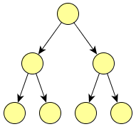
(a) fixed structure

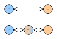
(b) operation average

Figure 1: Basic Ideas

So far, this yields a smooth optimization problem for the operator choices where only real values have to be adjusted. However, this simply replaces every operator with a weighted average of other operators and make the formula much more complicated. Therefore, another simple addition is necessary: The overall fitness function is augmented with a penalty for undecided operator choices. In the simplest possible case where two possible operators are chosen an inverted quadratic function that peaks at 0.5 and intersects with the abscissa at zero and one can be used. When more than two operations are available a different penalty function is required. In this case the least penalty should occur when exactly one operator is chosen and it should increase progressively the more weight other operators are receiving. Therefore, the simple formula shown in Equation 2 can been used to steer the optimization towards a unique operator choice.

$$p_{\mathrm{op}}(\alpha):=\left(\sum_{i}^{2^{d}-1}\alpha_{i}-\max_{i}\alpha_{i}\right)/(2^{d}-2)$$ (2)

Now that the structure and the operators of the tree can be selected using only real values, the last remaining aspect is how to make a smooth choices between variables. This task is a litte more complicated as the variables should also have a weight attached. However, another simple solution can be applied as shown in Equation 3 where the operation in the leaf node is selected in addition to the variables, and $n$ is the number of input variables in $X$. Please note that one additional weight $\beta_{i,n+1}$is included to allow a constant to be selected which gives the ability to “mute” parts of the tree by selecting for example a multiplication with one or an addition with zero for some subtree.

$$\mathrm{op}(X):=\sum_{i}^{2^{d-1}}\alpha_{i}\cdot\mathrm{op}(\beta_{i,1}\cdot X_{1},\ldots,\beta_{i,n}\cdot X_{n},\beta_{i,n+1})$$ (3)

This yields quite a large number of variable weights. As the number of leaf nodes increases exponentially with the tree depth and is further multiplied with the number of input variables. For example a smooth symbolic regression problem with ten variables and a tree depth of five has only 31 operator weights but 176 variable weights.

In Figure 2 several alternative ideas are shown for variable selection schemes with fewer resulting variables. However, they have not been very promising in preliminary tests. Therefore, we can only recommend to use the variable selection scheme with more variables, given the complexity of the variable selection problem per se. The first idea was to use only a single angle and take the two closest variables weighted by distance, as shown in Figure 2a, however, this blinds the algorithm by completely hiding other choices. This might still be a good option for other algorithms where diversity of the population is kept very high. Another idea was to use multidimensional scaling [1] to project the variables according to their correlation onto e.g. a two dimensional plane and use only two coordinates to choose between all variables. Figure 2b shows the selection of the two nearest neighbors, which has similar problems as the angular selection as it completely hides other variable choices. The second alternative is to use again a weighted average, however, using the distance to the coordinates as the weights.

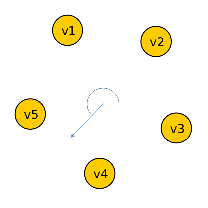
(a) angular

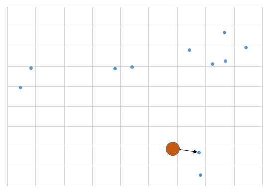
(b) nearest neighbor

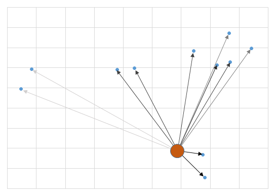
(c) weighted average

Figure 2: Alternative Variable Selection Strategies

It has to be noted, that also for the variable selection the optimization has to be guided towards limiting the number of variables. This can be achieved similarly to the operator choice, only that this time two or more non-zero weights are acceptable and their weights can be subtracted from the penalty.

In summary, the new encoding transforms a problem with $2^{d}-1$ tree nodes, where $d$ is the depth of the tree, $k$ possible operations at each node and $n$ input variables into a problem with $(2^{d}-1)\cdot(k-1)$ operator weights $\alpha$ and $(2^{d-1})\cdot n$ variable weights $\beta$. So, for example, for a depth of five, with two operations and ten variables we get a 31+176=207 dimensional real-valued problem instead of a combinatorial problem with $6\cdot 10^{20}$ possible choices. Obviously this does not make the problem less complex, i.e. dimensions compared with choices, however it makes the fitness landscape much smoother. One could think of discrete points in space in the combinatorial formulation and filling the volume between them in the smooth approach.

3 Experimental Results

We have tested this new implementation only on comparatively simple problems most notably the Poly-10 Problem [13] using custom operators in HeuristicLab [21] with a CMA Evolution Strategy[6]. One very interesting aspect is shown in Figure 3 where the penalties for operators and variable weights have been successively turned on. It can be seen that the correlation of the formula slightly decreases as the optimization tries to lower the operator penalty but quickly recovers with very low operator penalties, indicating a crisp operator choice. This choice is also achieved rather quickly indicating that it might not be so difficult to make this crisp operator choice. When turning on the variable selection penalty a distinct knee and steeper slope can be seen in the variable selection penalty curve, however, it is much harder to decrease as many more weights are involved.

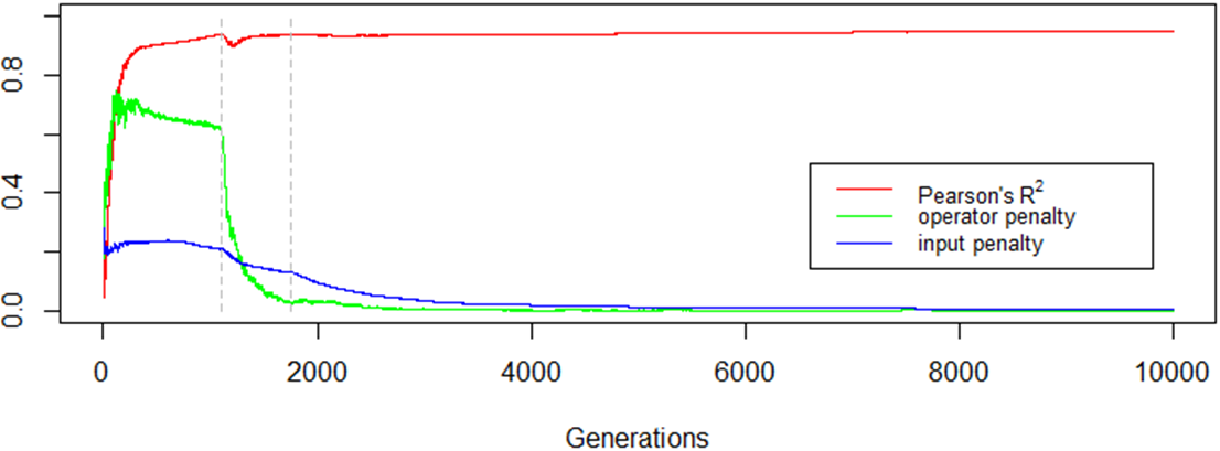
Figure 3: Results

Finally, we have used the new formulation to calculate some fitness landscape analysis measures. For the first time, traditional techniques can be applied to symbolic regression problems and reasonable results can be obtained as shown in Table 1, where the fitness landscape of the Poly-10 Problem was analyzed using different neighborhoods: In particular polynomial one position or all position manipulators where used with contiguity of 15 or only 2 as well as a uniform one position manipulator. Both random and up-down walks [8] where performed to get a first impression of the landscape’s characteristics.

Table 1: Fitness Landscape Analysis of Symbolic Regression Problem

	Poly-1-15	Poly-All-15	Poly-1-2	Poly-All-2	Uni-1
auto correlation	0.999	0.910	0.998	0.547	0.991
corr. length	2245	57	1246	11	290
density basin information	0.628	0.619	0.626	0.593	0.628
information content	0.546	0.394	0.686	0.403	0.399
information stability	0.058	0.141	0.058	0.255	0.037
partial inf. content	0.476	0.532	0.457	0.586	0.506
up walk length	328.063	124.872	14.321	5.179	83.433
up walk len. variance	46668.196	5405.852	35.814	3.176	870.758
down walk length	296.563	123.400	12.140	4.878	83.100
down walk len. variance	27152.263	4627.477	26.232	2.713	832.024

4 Conclusions

While there is certainly still a lot of work needed to fine tune the optimization process and play with different variants of variable selection and penalty schemes, this transformation principle opens the door for classical fitness landscape analysis applied to symbolic regression problems. The focus of future work should therefore not be the tuning of algorithm performance but rather the interpretation and utilization of FLA results generated for the class of symbolic regression problems.

Acknowledgments

The work described in this paper was done within the COMET Project Heuristic Optimization in Production and Logistics (HOPL), #843532 funded by the Austrian Research Promotion Agency (FFG).

References

- [1] Borg, I., Groenen, P.: Modern Multidimensional Scaling: theory and applications. New York: Springer-Verlag. (2005)
- [2] Chicano, F., Whitley, L.D., Alba, E., Luna, F.: Elementary landscape decomposition of the frequency assignment problem. Theoretical Computer Science 412, 6002–6019 (2011)
- [3] Cortes, C., Vapnik, V.: Support-vector networks. Machine Learning 20(3), 273–297 (1995)
- [4] Deng, L., Yu, D.: Deep Learning: Methods and Applications, Foundations and Trens in Signal Processing, vol. 7. Now Publishers Inc. (2013)
- [5] Freedman, D.A.: Statistical Models: Theory and Practice. Cambridge University Press (2009)
- [6] Hansen, N.: Towards a New Evolutionary Computation: Advances on Estimation of Distribution Algorithms, chap. The CMA evolution strategy: a comparing review, pp. 1769–1776. Springer (2006)
- [7] Hordijk, W.: A measure of landscapes. Evol. Comput. 4(4), 335–360 (1996)
- [8] Jones, T.: Evolutionary Algorithms, Fitness Landscapes and Search. Ph.D. thesis, University of New Mexico, Albuquerque, New Mexico (1995)
- [9] Keijzer, M.: Improving symbolic regression with interval arithmetic and linear scaling. In: Genetic Programming, 6th European Conference, EuroGP 2003, Essex, UK, April 14-16, 2003. Proceedings. pp. 70–82 (2003)
- [10] Kommenda, M., Kronberger, G., Winkler, S., Affenzeller, M., Wagner, S.: Effects of constant optimization by nonlinear least squares minimization in symbolic regression. In: GECCO ’13 Companion: Proceeding of the fifteenth annual conference companion on Genetic and evolutionary computation conference companion. pp. 1121–1128. ACM, Amsterdam, The Netherlands (2013)
- [11] Kotanchek, M., Smits, G., Vladislavleva, E.: Trustable symbolic regression models: using ensembles, interval arithmetic and pareto fronts to develop robust and trust-aware models. In: Riolo, R.L., Soule, T., Worzel, B. (eds.) Genetic Programming Theory and Practice V, chap. 12, pp. 201–220. Genetic and Evolutionary Computation, Springer (2007)
- [12] Koza, J.R.: Genetic Programming: On the Programming of Computers by Means of Natural Selection. MIT Press (1992)
- [13] Langdon, W.B., Banzhaf, W.: Repeated patterns in genetic programming. Natural Computing 7(4), 589–613 (2008)
- [14] McConaghy, T.: FFX: fast, scalable, deterministic symbolic regression technology. Genetic Programming Theory and Practice IX pp. 235–260 (2011)
- [15] Nelder, J., Wedderburn, R.: Generalized linear models. Journal of the Royal Statistical Society Series A (General) 135(3), 370–384 (1972)
- [16] Rosenblatt, F.: The perceptron: A probabilistic model for information storage and organization in the brain. Psychological Review 65(6), 386–408 (1958)
- [17] Stadler, P.F.: Linear operators on correlated landscapes. J.Phys.I France 4, 681–696 (1994)
- [18] Stadler, P., Wagner, G.: The algebraic theory of recombination spaces. Evol.Comp. 5, 241–275 (1998)
- [19] Vassilev, V.K., Fogarty, T.C., Miller, J.F.: Information characteristics and the structure of landscapes. Evol. Comput. 8(1), 31–60 (2000)
- [20] Vladislavleva, E.J., Smits, G.F., Hertog, D.D.: Order of nonlinearity as a complexity measure for models generated by symbolic regression via pareto genetic programming. IEEE Transactions on Evolutionary Computation 13(2), 333–349 (2009)
- [21] Wagner, S.: Heuristic Optimization Software Systems - Modeling of Heuristic Optimization Algorithms in the HeuristicLab Software Environment. Ph.D. thesis, Johannes Kepler University, Linz, Austria (2009)
- [22] Weinberger, E.: Correlated and uncorrelated fitness landscapes and how to tell the difference. Biological Cybernetics 63(5), 325–336 (1990)
- [23] Worm, T., Chiu, K.: Prioritized grammar enumeration: symbolic regression by dynamic programming. In: GECCO. pp. 1021–1028 (2013)