BiMaL: Bijective Maximum Likelihood Approach to
Domain Adaptation in Semantic Scene Segmentation

Abstract

Semantic segmentation aims to predict pixel-level labels. It has become a popular task in various computer vision applications. While fully supervised segmentation methods have achieved high accuracy on large-scale vision datasets, they are unable to generalize on a new test environment or a new domain well. In this work, we first introduce a new Unaligned Domain Score to measure the efficiency of a learned model on a new target domain in unsupervised manner. Then, we present the new Bijective Maximum Likelihood (BiMaL) loss that is a generalized form of the Adversarial Entropy Minimization without any assumption about pixel independence. We have evaluated the proposed BiMaL on two domains. The proposed BiMaL approach consistently outperforms the SOTA methods on empirical experiments on “SYNTHIA to Cityscapes”, “GTA5 to Cityscapes”, and “SYNTHIA to Vistas”.

1 Introduction

Semantic segmentation is one of the most popular computer vision topics, which aims to to assign each pixel in an image to a predefined class. It has various practical applications, especially in autonomous driving where a segmentation model is needed to recognize roads, sidewalks, pedestrians or vehicles in a large variety of urban conditions. A typical supervised segmentation model is usually trained on datasets with labels. However, annotating images for the semantic segmentation task is costly and time-consuming. Alternatively, a powerful and cost-effective way to acquire a large-scale training set is to use a simulation, e.g. game engines, to create a synthetic dataset [42, 43]. However, fully supervised models [3, 24] trained on the synthetic datasets are often unable to perform well on real images due to the pixel appearance gap between synthetic and real images.

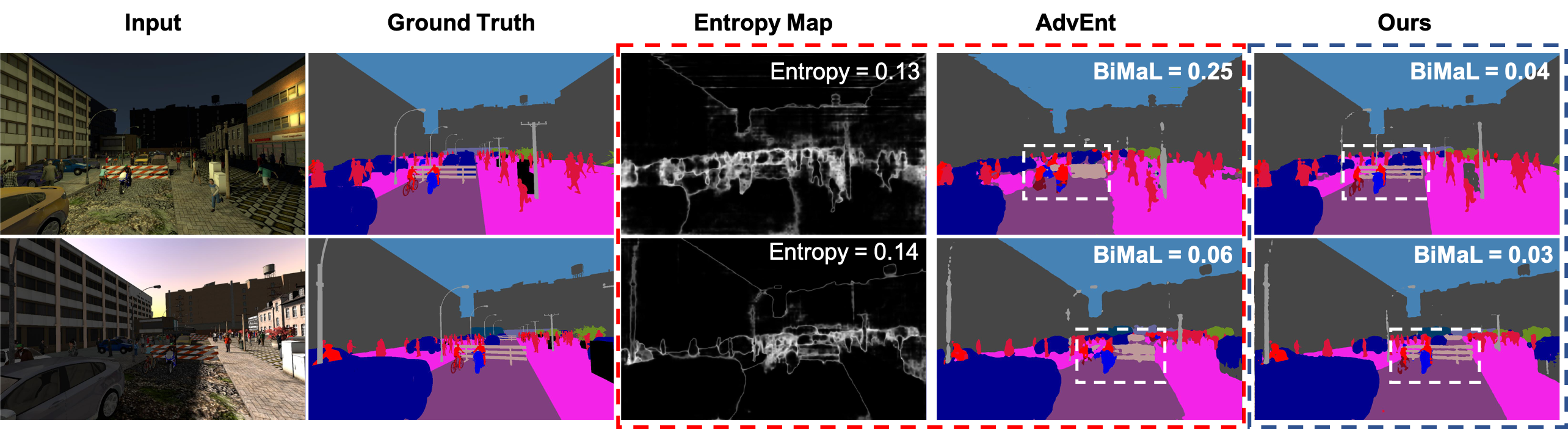
Figure 1: Two images have the same entropy but one has a poor prediction (a top image) and one has an better prediction (a bottom image). Columns 1 and 2 are an input image and a ground truth. Columns 3 and 4 are an entropy map and a prediction of AdvEnt [54]. Column 5 is the results of our proposed method. The two predictions produced by AdvEnt have similar entropy scores ($0.13$ and $0.14$). Meanwhile, the BiMaL value of the bottom prediction ($0.06$) is smaller than the top prediction ($0.14$). Our results in the last column, which have better BiMaL values than AdvEnt, can well model the structure of an image. In particular, our results have sharper results of a barrier and a rider (white dash box), and a clear boundary between road and sidewalk.

Unsupervised Domain Adaptation (UDA) aims to train a machine learning model on an annotated dataset, i.e. the source, and guarantee its high performance on a new unlabeled dataset, i.e. the target. The UDA approaches have been applied to various computer vision tasks such as Semantic Segmentation [3, 24, 26, 54, 55, 57], Face Recognition [12, 32, 33, 34, 35]. The recent UDA methods aim to reduce the cross-domain discrepancy, along with the supervised training on the source domain [5, 16, 29, 40, 52, 54]. In particular, these methods aim to minimize the distribution discrepancy of the deep representations extracted from the source and the target domains. This process can be performed at single or multiple levels of deep features using maximum mean discrepancies [16, 29, 52], or adversarial training [5, 6, 20, 21, 22, 50]. The approaches in this group have shown their potential in aligning the predicted outputs of images from the two domains. However, the binary cross-entropy label predicted by the learned discriminator is usually a weak indication of structural learning for the segmentation task. Another approach named self-training utilizes the pseudo-labels or generative networks conditioned on target images [37, 58]. Semi-supervised learning is an approach related to UDA where the training set consists of both labeled and unlabeled samples. Thus, it has motivated several UDA approaches such as Class-balanced self-training (CBST) [60], and entropy minimization [4, 17, 40, 47, 54]. Although metrics such as entropy can be efficiently computed and adopted for training, they tend to rely on easy predictions, i.e. high confident scores, as references for the label transfer from source to target domains. This issue is alleviated in a later approach [4] by preventing learned models from over-focusing on high confident areas. However, this type of metrics is formulated in pixel-wised manner, and, therefore, neglects the structural information presented in the image (see Figure 1).

Contributions of this Work. This work presents a new unsupervised domain adaptation approach to tackle the semantic segmentation problem. Table 1 summarizes the difference between our proposed approach and the prior ones. Our contributions can be summarized as follows.

Firstly, a new Unaligned Domain Score (UDS) is introduced to measure the efficiency of the learned model on a target domain in an unsupervised manner. Secondly, the presented UDS is further extended as a new loss function, named Bijective Maximum Likelihood (BiMaL) loss, that can be used with an unsupervised deep neural network to generalize on target domains. Indeed, we further demonstrate BiMaL loss is a generalized form of the Adversarial Entropy Minimization (AdvEnt) [54] without pixel independence assumption. Far apart from AdvEnt that assumes pixel independence, BiMaL loss is formed using a Maximum-likelihood formulation to model the global structure of a segmentation input and a Bijective function to map that segmentation structure to a deep latent space. Finally, the proposed BiMaL method is evaluated on three popular large-scale semantic segmentation benchmarks, including GTA5 [42] $to$ CityScapes [7], SYNTHIA [43] $to$ Cityscapes, and SYNTHIA $to$ Vista [38]. The experimental results demonstrate our proposed BiMaL approach consistently outperforms the State-of-the-Art (SOTA) methods [5, 40, 50, 54, 55] in all these benchmark databases. To the best of our knowledge, this is one of the first works that introduces a novel bijective maximum likelihood approach with flow-based metric to unsupervised domain adaptation in semantic segmentation.

2 Related Work

Unsupervised Domain Adaptation has recently become one of the most active research topics. The common UDA approaches are domain discrepancy minimization [16, 29, 52], adversarial learning [5, 6, 20, 21, 22, 50], entropy minimization [37, 40, 54, 58], self-training [60]. In the scope of this work, UDA is focused on semantic segmentation.

Adversarial training is the most common approach employed to UDA for semantic segmentation. Similar to generative adversarial networks (GANs), the adversarial training paradigm aims at training a discriminator to predict the domain of inputs while the segmentation network tries to fool the discriminator. This adversarial step is trained simultaneously with the supervised segmentation task on the source domain. Hoffman et al. [21] first introduced GAN-based UDA approach to semantic segmentation. Later, Chen et al. [6] presented global and class-wise adaptation learned by adversarial learning on pseudo labels. Considering the difference in spatial distribution, [5] proposed a spatial-aware adaptation method to align two domains along with a target guided distillation loss. Hong et al. [22] learned a conditional generator to transform the feature maps of source domain to be similar to target domain. Tasi et al. [50] used adversarial learning to learn a consistency of scene layout and local context between source and target domains. There are some prior methods that utilize the generative networks to synthesize target images conditioned on source images [58, 37]. Hoffman et al. [20] presented Cycle-Consistent Adversarial Domain Adaptation that aligns at both pixel-level and feature-level representations. Zhu et al. [59] introduced a conservative loss in an adversarial framework that penalizes the easy and hard source examples. We et al. [56] proposed a DCAN framework that uses the channel-wise feature alignment in the segmentation networks. Sakaridis et al. [44] proposed an UDA framework on scene understanding that gradually adapts a segmentation model from non-foggy to heavy-foggy images.

Table 1: Comparison in the properties between our proposed approach and other methods. Convolutional Neural Network (CNN), Generative Adversarial Net (GAN), Bijective Network (BiN), Entropy Minimization (EntMin), Curriculum Training (CT), Image-wise Weighting (IW), Segmentation Map (Seg), Depth Map (Depth); $\ell_{CE}$: Cross-entropy Loss, $\ell_{adv}$: Adversarial Loss, $\ell_{Huber}$: Huber Loss.

Methods	Architecture	Source Label	Learning Mechanism	Loss Function	Structural Learning
AdaptSeg [50]	CNN + GAN	Seg	Domain Adaptation	$\ell_{adv}$	Weak (binary label)
AdaptPatch [51]	CNN + GAN	Seg	Domain Adaptation	$\ell_{adv}$	Weak (binary label)
CBST [60]	CNN	Seg	Self-Training	$\ell_{CE}$	Not Applicable
ADVENT [54]	CNN + GAN	Seg	Domain Adaptation	EntMin	Weak (binary label)
MaxSquare [4]	CNN + GAN	Seg	Domain Adaptation	Squares loss + IW	Weak (binary label)
IntraDA [40]	CNN + GAN	Seg	Curriculum Learning	EntMin	Weak (binary label)
SPIGAN [25]	CNN + GAN	Seg + Depth	Domain Adaptation	$\ell_{adv}$ + $\ell_{1}$	Weak (binary label)
DADA [55]	CNN + GAN	Seg + Depth	Domain Adaptation	$\ell_{adv}$ + $\ell_{Huber}$	Depth-aware Label
BiMaL	CNN + BiN	Seg	Domain Adaptation	Maximum Likelihood	Segmentation Density (Unsupervised)

To enhance the performance of domain adaptation, several methods explore the use of privileged information available on source data [2, 27, 45]. Vapnik et al. [53] first introduced the idea of privileged information, i.e. additional information only available at the training process. Later, many methods [19, 30, 36, 46] take advantage of privileged information for various tasks. In semantic segmentation, SPIGAN [25] proposed an UDA approach that utilizes the depth information during the training phase. Following SPIGAN, Vu et al. [55] presented an adversarial approach that utilizes the depth-aware of source and target images.

Entropy minimization has been used for semi-supervised learning [17, 47]. Vu et al. [54] first introduced the entropy minimization approach for domain adaptation in semantic segmentation. The minimization process is solved by adversarial learning. Later, [40] introduced an intra-domain adaptation approach based on the entropy level of predictions. The learning process involves two phases. The first phase performs adaptation from the source domain to the target domain, whereas the second phase aligns the hard split and easy split within the target domain. Another recent UDA approach is self-training, where the predictions of the trained model are used as pseudo-labels for the unlabeled data to train the new model. Self-training has been widely used in classification [28] and segmentation tasks [60].

3 Unaligned Domain Scores (UDS)

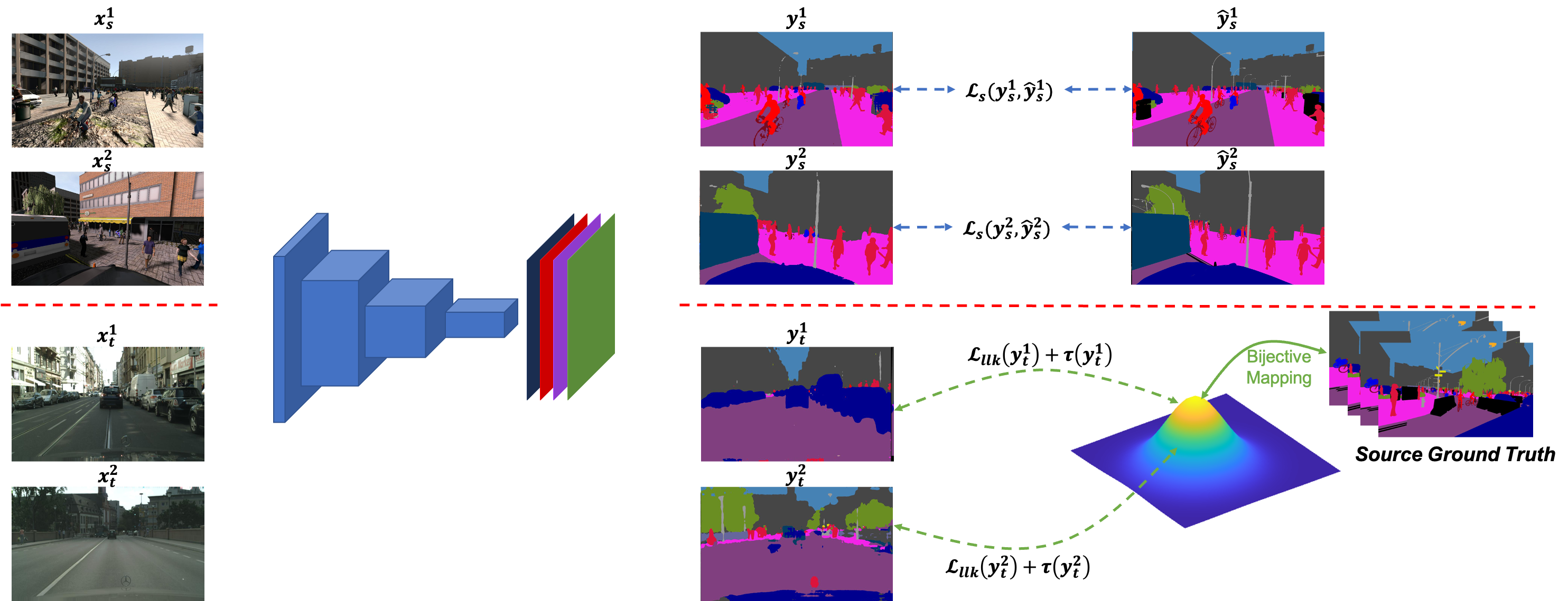
Figure 2: The Proposed Framework. The RGB image input is firstly forwarded to a deep semantic segmentation network to produce a segmentation map. The supervised loss is employed on the source training samples. Meanwhile, the predicted segmentation on target training samples will be mapped to the latent space to compute the Bijective Maximum Likelihood loss. The bijective mapping network is trained on the ground-truth images of the source domain.

Let $\mathbf{x}_{s}\in\mathcal{X}_{s}\subset\mathbb{R}^{H\times W\times 3}$ be an input image of the source domain ($H$ and $W$ are the height and width of an image), $\mathbf{x}_{t}\in\mathcal{X}_{t}\subset\mathbb{R}^{H\times W\times 3}$ be an input image of the target domain, $G:\mathcal{X}\to\mathcal{Y}$ where $\mathcal{X}=\mathcal{X}_{s}\cup\mathcal{X}_{t}$ be a semantic segmentation function that maps an input image to its corresponding segmentation map $\mathbf{y}\subset\mathbb{R}^{H\times W\times C}$, i.e. $\mathbf{y}=G(\mathbf{x},\theta)$ ($C$ is the number of semantic classes). In general, given $N$ labeled training samples from a source domain $\mathcal{D}_{s}=\{\mathbf{x}_{s}^{i},\hat{\mathbf{y}}_{s}^{i}\}_{1}^{N}$ and $M$ unlabeled samples from a target domain $\mathcal{D}_{t}=\{\mathbf{x}_{t}^{i}\}_{1}^{M}$, the unsupervised domain adaptation for semantic segmentation can be formulated as:

$$\small\begin{split}\theta^{*}&=\arg\min_{\theta}\sum_{i,j}\big{[}\mathcal{L}_{s}(G(\mathbf{x}^{i}_{s},\theta),\hat{\mathbf{y}}^{i}_{s})+\mathcal{L}_{t}(G(\mathbf{x}^{j}_{t},\theta))\big{]}\\ &=\arg\min_{\theta}\Big{[}\mathbb{E}_{\mathbf{x}_{s}\sim p(\mathbf{x}_{s}),\hat{\mathbf{y}}_{s}\sim p(\hat{\mathbf{y}}_{s})}\big{[}\mathcal{L}_{s}(G(\mathbf{x}_{s},\theta),\hat{\mathbf{y}}_{s})]\\ &\quad\quad\quad\quad+\mathbb{E}_{\mathbf{x}_{t}\sim p(\mathbf{x}_{t})}[\mathcal{L}_{t}(G(\mathbf{x}_{t},\theta))\big{]}\Big{]}\\ &=\arg\min_{\theta}\Big{[}\mathbb{E}_{\mathbf{y}_{s}\sim p(\mathbf{y}_{s}),\hat{\mathbf{y}}_{s}\sim p(\hat{\mathbf{y}}_{s})}\big{[}\mathcal{L}_{s}(\mathbf{y}_{s},\hat{\mathbf{y}}_{s})]\\ &\quad\quad\quad\quad+\mathbb{E}_{\mathbf{y}_{t}\sim p(\mathbf{y}_{t})}[\mathcal{L}_{t}(\mathbf{y}_{t})\big{]}\Big{]}\\ \end{split}$$ (1)

where $\theta$ is the parameters of $G$, $p(\mathbf{\cdot})$ is the probability density function. As the labels for $\mathcal{D}_{s}$ are available, $\mathcal{L}_{s}$ can be efficiently formulated as a supervised cross-entropy loss:

$$\small\mathcal{L}_{s}(\mathbf{y}_{s},\hat{\mathbf{y}}_{s})=-\sum_{h,w,c}\hat{\mathbf{y}}^{h,w,c}_{s}\log\left(\mathbf{y}^{h,w,c}_{s}\right)$$ (2)

where $\mathbf{y}^{h,w,c}$ and $\hat{\mathbf{y}}^{h,w,c}$ represent the predicted and ground-truth probabilities of the pixel at the location of $(h,w)$ taking the label of $c$ , respectively. Meanwhile, $\mathcal{L}_{t}$ handles unlabeled data from the target domain where the ground-truth labels are not available. To alleviate this label lacking issue, several forms of $\mathcal{L}_{t}(\mathbf{y}_{t})$ have been exploited such as cross-entropy loss with pseudo-labels [60], Probability Distribution Divergence (i.e. Adversarial loss defined via an additional Discriminator) [50, 51], or entropy formulation [54, 40].

Entropy minimization revisited. By adopting the Shannon entropy formulation to the target prediction and constraining function $G$ to produce a high-confident prediction, $\mathcal{L}_{t}$ can be formulated as

$$\small\mathcal{L}_{t}(\mathbf{y}_{t})=\frac{-1}{\log(C)}\sum_{h,w,c}\mathbf{y}^{h,w,c}_{t}\log\left(\mathbf{y}^{h,w,c}_{t}\right).$$ (3)

Although this form of $\mathcal{L}_{t}$ can give a direct assessment of the predicted segmentation maps, it tends to be dominated by the high probability areas (since the high probability areas produce a higher value updated gradient due to $\lim_{\mathbf{y}^{h,w,c}_{t}\to 1}\frac{-\partial\mathcal{L}_{t}(\mathbf{y}_{t})}{\partial\mathbf{y}^{h,w,c}_{t}}=\frac{1}{\log(C)}$ and $\lim_{\mathbf{y}^{h,w,c}_{t}\to 0}\frac{-\partial\mathcal{L}_{t}(\mathbf{y}_{t})}{\partial\mathbf{y}^{h,w,c}_{t}}=-\infty$), i.e. easy classes, rather than difficult classes [54]. More importantly, this is essentially a pixel-wise formation, where pixels are treated independently of each other. Consequently, the structural information is usually neglected in this form. This issue could lead to a confusion point during training process where two predicted segmentation maps have similar entropy but different segmentation accuracy, one correct and other incorrect as shown in Fig 1.

3.1 The Proposed UDS Metric

In the entropy formulation, the pixel independent constraints are employed to convert the image-level metric to pixel-level metric. In contrast, we propose an image-level UDS metric that can directly evaluate the structural quality of $\mathbf{y}_{t}$. Particularly, let $p_{t}(\mathbf{y}_{t})$ and $q_{t}(\mathbf{y}_{t})$ be the probability mass functions of the predicted distribution and the real (actual) distribution of the predicted segmentation map $\mathbf{y}_{t}$, respectively. UDS metric measuring the efficiency of function $G$ on the target dataset can be expressed as follows:

$$\begin{split}\operatorname{UDS}&=\mathbb{E}_{\mathbf{y}_{t}\sim p(\mathbf{y}_{t})}\mathcal{L_{Y}}\left(p_{t}(\mathbf{y}_{t}),q_{t}(\mathbf{y}_{t})\right)\\ &=\int\mathcal{L_{Y}}\left(p_{t}(\mathbf{y}_{t}),q_{t}(\mathbf{y}_{t})\right)p_{t}(\mathbf{y}_{t})d\mathbf{y}_{t}\;,\end{split}$$ (4)

where $\mathcal{L_{Y}}\left(p_{t}(\mathbf{y}_{t}),q_{t}(\mathbf{y}_{t})\right)$ defines the distance between two distributions $p_{t}(\mathbf{y}_{t})$ and $q_{t}(\mathbf{y}_{t})$. Since there is no label for sample in the target domain, the direct access to $q_{t}(\mathbf{y}_{t})$ is not available. Note that although $\mathbf{x}_{s}$ and $\mathbf{x}_{t}$ could vary significantly in image space (e.g. difference in pixel appearance due to lighting, scenes, weather), their segmentation maps $\mathbf{y}_{t}$ and $\mathbf{y}_{s}$ share similar distributions in terms of both class distributions as well as global and local structural constraints (sky has to be above roads, trees should be on sidewalks, vehicles should be on roads, etc.). Therefore, one can practically adopted the prior knowledge learned from segmentation labels of the source domains for $q_{t}(\mathbf{y}_{t})$ as

$$\begin{split}\operatorname{UDS}&\approx\int\mathcal{L_{Y}}\left(p_{t}(\mathbf{y}_{t}),q_{s}(\mathbf{y}_{t})\right)p_{t}(\mathbf{y}_{t})d\mathbf{y}_{t}\;,\end{split}$$ (5)

where the distribution $q_{s}(\mathbf{y}_{t})$ is the probability mass functions of the real distribution learned from ground-truth segmentation maps of $\mathcal{D}_{s}$. As a result, the proposed USD metric can be computed without the requirement of labeled target data for learning the density of segmentation maps in target domain. There are several choices for $\mathcal{L_{Y}}$ to estimate the divergence between the two distributions $p_{t}(\mathbf{y}_{t})$ and $q_{s}(\mathbf{y}_{t})$. In this paper, we adopt the common metric such as Kullback–Leibler (KL) formula for $\mathcal{L_{Y}}$. Note that other metrics are also applicable in the proposed UDS formulation. Moreover, to enhance the smoothness of the predicted semantic segmentation, a regularization term $\tau$ is imposed into $\mathcal{L_{Y}}$ as

$$\begin{split}\small\mathcal{L_{Y}}\left(p_{t}(\mathbf{y}_{t}),q_{s}(\mathbf{y}_{t})\right)&=\log\left(\frac{p_{t}(\mathbf{y}_{t})}{q_{s}(\mathbf{y}_{t})}\right)+\tau(\mathbf{y}_{t}).\\ \end{split}$$ (6)

By computing UDS, one can measure the quality of the predicted segmentation maps $\mathbf{y}_{t}$ on the target data.

In the next sections, we firstly discuss in details the learning process of $q_{s}(\mathbf{y}_{t})$, and then derivations of the UDS metric for the novel Bijective Maximum Likelihood loss.

3.2 Learning Distribution with Bijective Mapping on the Source Domain

Let $F:\mathcal{Y}\to\mathcal{Z}$ be the bijective mapping function that maps a segmentation $\hat{\mathbf{y}}_{s}\in\mathcal{Y}$ to the latent space $\mathcal{Z}$, i.e. $\hat{\mathbf{z}}_{s}=F(\hat{\mathbf{y}}_{s},\theta_{F})$, where $\hat{\mathbf{z}}_{s}\sim q_{z}(\hat{\mathbf{z}}_{s})$ is the latent variable, and $q_{z}$ is the prior distribution. Then, the probability distribution $q_{s}(\hat{\mathbf{y}}_{s})$ can be formulated via the change of variable formula:

$$\small\log(q_{s}(\hat{\mathbf{y}}_{s}))=\log\left(q_{z}(\hat{\mathbf{z}}_{s})\right)+\log\left(\left|\frac{\partial F(\hat{\mathbf{y}}_{s},\theta_{F})}{\partial\hat{\mathbf{y}}_{s}}\right|\right),$$ (7)

where $\theta_{F}$ is the parameters of $F$, $\left|\frac{\partial F(\hat{\mathbf{y}}_{s},\theta_{F})}{\partial\hat{\mathbf{y}}_{s}}\right|$ denotes the Jacobian determinant of function $F(\hat{\mathbf{y}}_{s},\theta_{F})$ with respect to $\hat{\mathbf{y}}_{s}$. To learn the mapping function, the negative log-likelihood will be minimized as follows:

$$\footnotesize\begin{split}\theta_{F}^{*}=&\arg\min_{\theta_{F}}\mathbb{E}_{\hat{\mathbf{y}}_{s}\sim q_{s}(\hat{\mathbf{y}}_{s})}\Big{[}-\log(q_{s}(\hat{\mathbf{y}}_{s}))\Big{]}\\ =&\arg\min_{\theta_{F}}\mathbb{E}_{\hat{\mathbf{z}}_{s}\sim q_{z}(\hat{\mathbf{z}}_{s})}\left[-\log\left(q_{z}(\hat{\mathbf{z}}_{s})\right)-\log\left(\left|\frac{\partial F(\hat{\mathbf{y}}_{s},\theta_{F})}{\partial\hat{\mathbf{y}}_{s}}\right|\right)\right].\end{split}$$ (8)

In general, there are various choices for the prior distribution $q_{z}$. However, the ideal distribution should satisfy two criteria: (1) simplicity in the density estimation, and (2) easy in sampling. Considering the two criteria, we choose Normal distribution as the prior distribution $q_{z}$. Note that any other distribution is also feasible as long as it satisfies the mentioned criteria.

To enforce the information flow from a segmentation domain to a latent space with different abstraction levels, the bijective function $F$ can be further formulated as a composition of several sub-bijective functions $f_{i}$ as $F=f_{1}\circ f_{2}\circ...\circ f_{K}$, where $K$ is the number of sub-functions. The Jacobian $\frac{\partial F}{\partial\mathbf{y}_{s}}$ can be derived by $\frac{\partial F}{\partial\hat{\mathbf{y}}_{s}}=\frac{\partial f_{1}}{\partial\hat{\mathbf{y}}_{s}}\cdot\frac{\partial f_{2}}{\partial f_{1}}\cdots\frac{\partial f_{K}}{\partial f_{K-1}}$. With this structure, the properties of each $f_{i}$ will define the properties for the whole bijective mapping function $F$. Interestingly, with this form, $F$ becomes a DNN structure when $f_{i}$ is a non-linear function built from a composition of convolutional layers. Several DNN structures [8, 9, 39, 15, 23, 14, 49] can be adopted for sub-functions.

4 Bijective Maximum Likelihood Loss

In this section, we present the proposed Bijective Maximum Likelihood (BiMaL) which can be used as the loss of target domain $\mathcal{L}_{t}$. From Eqns. (5) and (6), UDS metric can be rewritten as follows:

$$\small\begin{split}\text{UDS}&=\int\left[\log\left(\frac{p_{t}(\mathbf{y}_{t})}{q_{s}(\mathbf{y}_{t})}\right)+\tau(\mathbf{y}_{t})\right]p_{t}(\mathbf{y}_{t})d\mathbf{y}_{t}\\ &={\mathbb{E}}_{\mathbf{y}_{t}\sim p_{t}(\mathbf{y}_{t})}\left[\log(p_{t}(\mathbf{y}_{t}))\right]\\ &\quad-{\mathbb{E}}_{\mathbf{y}_{t}\sim p_{t}(\mathbf{y}_{t})}\left[\log(q_{s}(\mathbf{y}_{t}))\right]+{\mathbb{E}}_{\mathbf{y}_{t}\sim p_{t}(\mathbf{y}_{t})}\left[\tau(\mathbf{y}_{t})\right]\\ &\leq{\mathbb{E}}_{\mathbf{y}_{t}\sim p_{t}(\mathbf{y}_{t})}\left[-\log(q_{s}(\mathbf{y}_{t}))+\tau(\mathbf{y}_{t})\right]\end{split}$$ (9)

It should be noticed that with any form of the distribution $p_{t}$, the above inequality still holds as $p_{t}(\mathbf{y}_{t})\in[0,1]$ and $\log(p_{t}(\mathbf{y}_{t}))\leq 0$. Now, we define our Bijective Maximum Likelihood Loss as

$$\begin{split}\mathcal{L}_{t}(\mathbf{y}_{t})=-\log(q_{s}(\mathbf{y}_{t}))+\tau(\mathbf{y}_{t}),\end{split}$$ (10)

where $\log(q_{s}(\mathbf{y}_{t}))$ defines the log-likelihood of $\mathbf{y}_{t}$ with respect to the density function $q_{s}$. Then, by adopting the bijectve function $F$ learned from Eqn. (8) using samples from source domain and the prior distribution $q_{z}$, the first term of $\mathcal{L}_{t}(\mathbf{y}_{t})$ in Eqn. (10) can be efficiently computed via log-likelihood formulation:

$$\small\begin{split}\mathcal{L}_{llk}(\mathbf{y}_{t})&=-\log(q_{s}(\mathbf{y}_{t}))\\ &=-\log\left(q_{z}(\mathbf{z}_{t})\right)-\log\left(\left|\frac{\partial F(\mathbf{y}_{t},\theta_{F})}{\partial\mathbf{y}_{t}}\right|\right),\end{split}$$ (11)

where $\mathbf{z}_{t}=F(\mathbf{y}_{t},\theta_{F})$. Thanks to the bijective property of the mapping function $F$, the minimum negative log-likelihood loss $\mathcal{L}_{llk}(\mathbf{y}_{t})$ can be effectively computed via the density of the prior distribution $q_{z}$ and its associated Jacobian determinant $\left|\frac{\partial F(\mathbf{y}_{t},\theta_{F})}{\partial\mathbf{y}_{t}}\right|$. For the second term of $\mathcal{L}_{t}(\mathbf{y}_{t})$, we further enhance the smoothness of the predicted semantic segmentation with the pair-wised formulation to encourage similar predictions for neighbourhood pixels with similar color:

$$\scriptsize\tau(\mathbf{y}_{t})=\sum_{h,w}\sum_{h^{\prime},w^{\prime}}\exp\left\{-\frac{||\mathbf{x}_{t}^{h,w}-\mathbf{x}_{t}^{h^{\prime},w^{\prime}}||_{2}^{2}}{2\sigma_{1}^{2}}-\frac{||\mathbf{y}_{t}^{h,w}-\mathbf{y}_{t}^{h^{\prime},w^{\prime}}||_{2}^{2}}{2\sigma_{2}^{2}}\right\}$$ (12)

where $(h^{\prime},w^{\prime})\in\mathcal{N}_{h,w}$ denotes the neighbourhood pixels of $(h,w)$, $\mathbf{x}^{h,w}$ represents the color at pixel $(h,w)$; and $\{\sigma_{1},\sigma_{2}\}$ are the hyper parameters controlling the scale of Gaussian kernels. It should be noted that any regularizers [3, 13] enhancing the smoothness of the segmentation results can also be adopted for $\tau$. Putting Eqns. (10), (11), (12) to Eqn (1), the objective function can be rewritten as:

$$\small\begin{split}\theta^{*}=\arg\min_{\theta}\Big{[}&\mathbb{E}_{\mathbf{y}_{s}\sim p(\mathbf{y}_{s}),\hat{\mathbf{y}}_{s}\sim p(\hat{\mathbf{y}}_{s})}\big{[}\mathcal{L}_{s}(\mathbf{y}_{s},\hat{\mathbf{y}}_{s})]\\ &+\mathbb{E}_{\mathbf{y}_{t}\sim p(\mathbf{y}_{t})}[\mathcal{L}_{llk}(\mathbf{y}_{t})+\tau(\mathbf{y}_{t})\big{]}\Big{]}\end{split}$$ (13)

Figure 2 illustrates our proposed BiMaL framework to learn the deep segmentation network $G$. Also, we can prove that direct entropy minimization as Eqn. (3) is just a particular case of our log likelihood maximization. We will further discuss how our maximum likelihood can cover the case of pixel-independent entropy minimization in Section 4.2.

4.1 BiMaL properties

Global Structure Learning. Sharing similar property with [10, 11, 15, 39, 48], from Eqn. (7), as the learned density function is adopted for the entire segmentation map $\hat{\mathbf{y}}_{s}$, the global structure in $\hat{\mathbf{y}}_{s}$ can be efficiently captured and modeled.

Tractability and Invertibility. Thanks to the designed bijection F, the complex distribution of segmentation maps can be efficiently captured. Moreover, the mapping function is bijective, and, therefore, both inference and generation are exact and tractable.

4.2 Relation to Entropy Minimization

The first term of UDS in Eqn. (9) can be derived as

$$\small\begin{split}&\int\log\left(\frac{p_{t}(\mathbf{y})}{q_{s}(\mathbf{y})}\right)p_{t}(\mathbf{y}_{t})d\mathbf{y}_{t}\geq 0\\ \Leftrightarrow&{\mathbb{E}}_{\mathbf{y}_{t}\sim p_{t}(\mathbf{y}_{t})}\left[\log(p_{t}(\mathbf{y}_{t}))-\log(q_{s}(\mathbf{y}_{t}))\right]\geq 0\\ \Leftrightarrow&{\mathbb{E}}_{\mathbf{y}_{t}\sim p_{t}(\mathbf{y}_{t})}\left[-\log(q_{s}(\mathbf{y}_{t}))\right]\geq{\mathbb{E}}_{\mathbf{y}_{t}\sim p_{t}(\mathbf{y}_{t})}\left[-\log(p_{t}(\mathbf{y}_{t}))\right]\\ \Leftrightarrow&\mathbb{E}_{\mathbf{y}_{t}\sim p_{t}(\mathbf{y}_{t})}[\mathcal{L}_{llk}(\mathbf{y}_{t})]\geq\text{Ent}(\mathbf{Y}_{t})\end{split}$$ (14)

where $\mathbf{Y}_{t}$ is the random variable with possible values $\mathbf{y}_{t}\sim p_{t}(\mathbf{y}_{t})$, and $\text{Ent}(\mathbf{Y}_{t})$ denotes the entropy of the random variable $\mathbf{Y}_{t}$. It can be seen that the proposed negative log-likelihood $\mathcal{L}_{llk}$ is an upper bound of the entropy of $\mathbf{Y}_{t}$. Therefore, minimizing our proposed BiMaL loss will also enforce the entropy minimization process. Moreover, by not assuming pixel independence, our proposed BiMaL can model and evaluate structural information at the image-level better than previous pixel-level approaches [4, 40, 54].

5 Experimental Results

This section will present our experimental results on three different benchmarks, i.e. SYNTHIA $to$ Cityscapes, GTA $to$ Cityscapes, and SYNTHIA $to$ Vistas. First, we overview datasets and network architectures used in our experiments. Second, we present the ablation study to analyze the effectiveness of our proposed BiMaL and the capability of the bijective network. Finally, we present the quantitative and qualitative results of our method compared to prior methods on the three benchmarks.

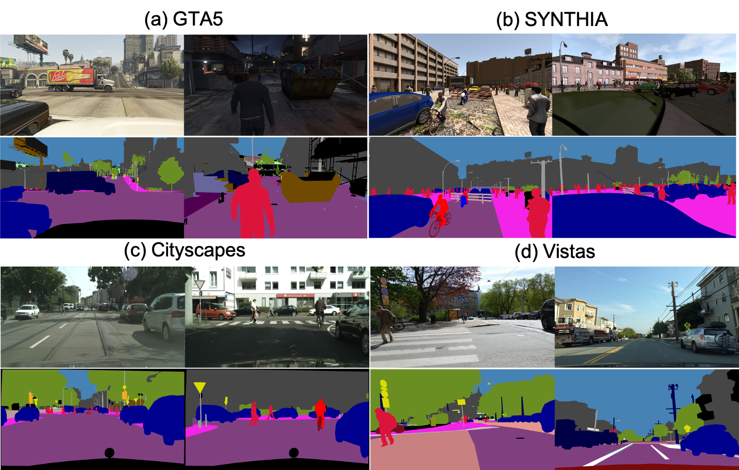
Figure 3: Examples of four semantic segmentation datasets including RGB images (top row) and corresponding ground-truth images (bottom row). (a) GTA and (b) SYNTHIA are synthetic datasets, (c) Cityscapes and (d) Vistas are real collected datasets.

5.1 Datasets

GTA5 [42] is a synthetic dataset containing $24,966$ densely labelled images at the resolution of $1,914\times 1,052$. This dataset was collected from the game Grand Theft Auto V. The ground-truth annotations were automatically generated with 33 categories. In our experiments, we consider 19 categories that are compatible with the Cityscapes [7].

SYNTHIA (SYNHIA-RAND-CITYSCAPES) [43] is also synthetic dataset that contains $9,400$ pixel-level labelled RGB images. In our experiments, we use the 16 common categories that overlap with the Cityscapes dataset.

Cityscapes [7] is a real-world dataset including $3,975$ images with fine semantic, dense pixel annotations of 30 classes. In our experiments, $2,495$ images are used for training and $500$ images are used for testing.

Vistas (Mapillary Vistas Dataset) [38] is diverse street-level imagery dataset with pixel‑accurate and instance‑specific human annotations for understanding street scenes around the world. Vistas consists of $25,000$ high-resolution images and $124$ semantic object categories. In our experiments, we consider 7 classes that are common to SYNTHIA, Cityscapes and Vistas as shown in Fig. 3.

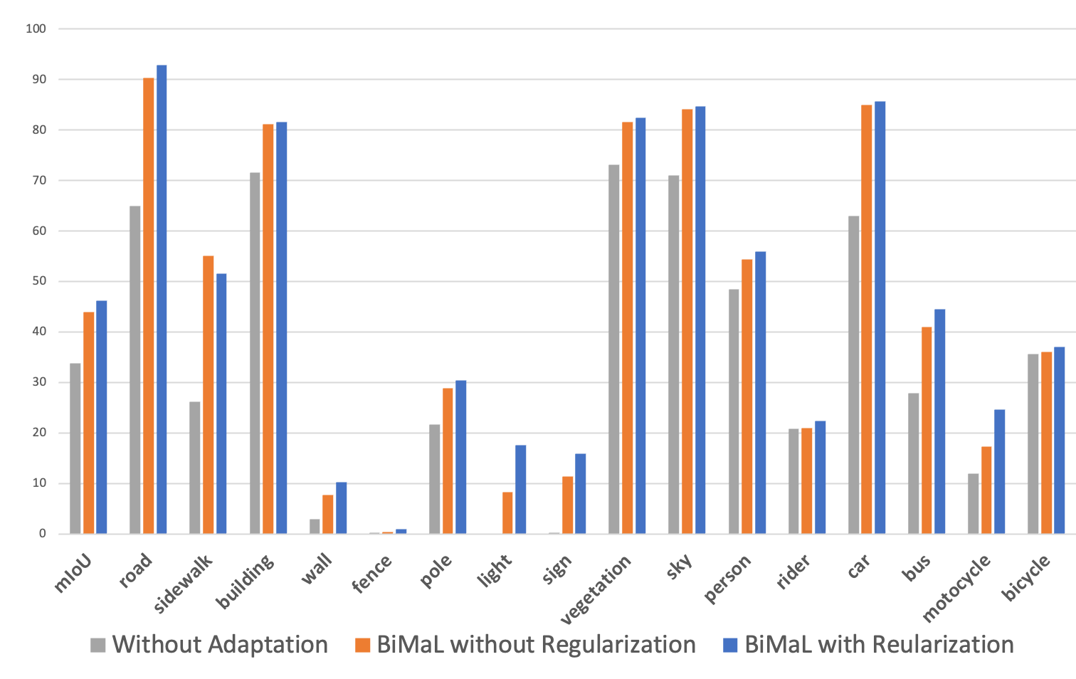
Figure 4: Ablative semantic segmentation performance mIoU (%) on the effectiveness of the proposed BiMaL loss.

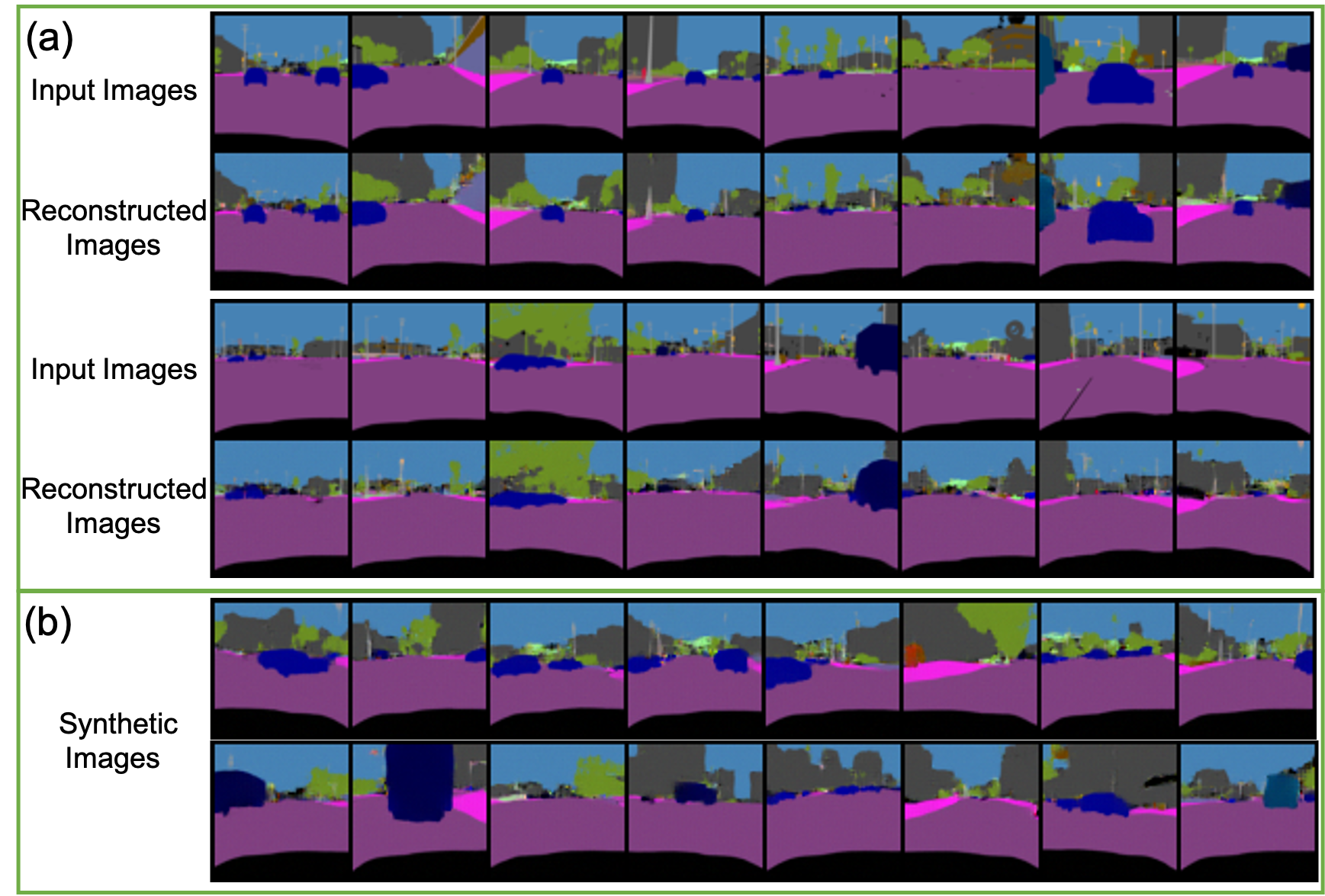
Figure 5: Reconstructed Images and Synthetic Images From The Bijective Mapping Function $F$. (a) Reconstructed images (bottom row) from the corresponding input images (top row). (b) Synthetic images sampled from the latent space.

Table 2: Semantic segmentation performance mIoU (%) on Cityscapes validation set of different models trained on SYNTHIA. We also show the mIoU (%) of the $13$ classes (mIoU*) excluding classes with *.

SYNTHIA $\rightarrow$ Cityscapes (16 classes)
Models	road	sidewalk	building	wall*	fence*	pole*	light	sign	veg	sky	person	rider	car	bus	mbike	bike	mIoU	mIoU*
Without Adaptation	64.9	26.1	71.5	3.0	0.2	21.7	0.1	0.2	73.1	71.0	48.4	20.7	62.9	27.9	12.0	35.6	33.7	39.6
SPIGAN-no-PI [25]	69.5	29.4	68.7	4.4	0.3	32.4	5.8	15.0	81.0	78.7	52.2	13.1	72.8	23.6	7.9	18.7	35.8	41.2
SPIGAN [25]	71.1	29.8	71.4	3.7	0.3	33.2	6.4	15.6	81.2	78.9	52.7	13.1	75.9	25.5	10.0	20.5	36.8	42.4
AdaptSegnet [50]	79.2	37.2	78.8	-	-	-	9.9	10.5	78.2	80.5	53.5	19.6	67.0	29.5	21.6	31.3	-	45.9
AdaptPatch [51]	82.2	39.4	79.4	-	-	-	6.5	10.8	77.8	82.0	54.9	21.1	67.7	30.7	17.8	32.2	-	46.3
CLAN [31]	81.3	37.0	80.1	-	-	-	16.1	13.7	78.2	81.5	53.4	21.2	73.0	32.9	22.6	30.7	-	47.8
AdvEnt [54]	87.0	44.1	79.7	9.6	0.6	24.3	4.8	7.2	80.1	83.6	56.4	23.7	72.7	32.6	12.8	33.7	40.8	47.6
IntraDA [40]	84.3	37.7	79.5	5.3	0.4	24.9	9.2	8.4	80.0	84.1	57.2	23.0	78.0	38.1	20.3	36.5	41.7	48.9
DADA[55]	89.2	44.8	81.4	6.8	0.3	26.2	8.6	11.1	81.8	84.0	54.7	19.3	79.7	40.7	14.0	38.8	42.6	49.8
Our BiMaL	92.8	51.5	81.5	10.2	1.0	30.4	17.6	15.9	82.4	84.6	55.9	22.3	85.7	44.5	24.6	38.8	46.2	53.7

Table 3: Semantic segmentation performance mIoU (%) on Cityscapes validation set of different models trained on GTA5

GTA5 $\to$ Cityscapes (19 classes)
Models	road	sidewalk	building	wall	fence	pole	light	sign	veg	terrain	sky	person	rider	car	truck	bus	train	mbike	bike	mIoU
Without Adaptation [50]	75.8	16.8	77.2	12.5	21.0	25.5	30.1	20.1	81.3	24.6	70.3	53.8	26.4	49.9	17.2	25.9	6.5	25.3	36.0	36.6
ROAD [5]	76.3	36.1	69.6	28.6	22.4	28.6	29.3	14.8	82.3	35.3	72.9	54.4	17.8	78.9	27.7	30.3	4.0	24.9	12.6	39.4
AdaptSegNet [50]	86.5	36.0	79.9	23.4	23.3	23.9	35.2	14.8	83.4	33.3	75.6	58.5	27.6	73.7	32.5	35.4	3.9	30.1	28.1	42.4
MinEnt [54]	84.2	25.2	77.0	17.0	23.3	24.2	33.3	26.4	80.7	32.1	78.7	57.5	30.0	77.0	37.9	44.3	1.8	31.4	36.9	43.1
AdvEnt [54]	89.9	36.5	81.6	29.2	25.2	28.5	32.3	22.4	83.9	34.0	77.1	57.4	27.9	83.7	29.4	39.1	1.5	28.4	23.3	43.8
Our BiMaL	91.2	39.6	82.7	29.4	25.2	29.6	34.3	25.5	85.4	44.0	80.8	59.7	30.4	86.6	38.5	47.6	1.2	34.0	36.8	47.3

5.2 Network Architectures

In our experiments, we adopt the DeepLab-V2 [3] with ResNet-101 [18] backbone for the segmentation network $G$. Also, we utilize the Atrous Spatial Pyramid Pooling with sampling rate $\{6,12,18,24\}$. We only use the output of layer conv5 to predict the segmentation. In the Bijective network $F$, we use the multi-scale architecture as [8, 9, 14, 23, 39]. For each scale, we have multiple steps of flow, each of which consists of ActNorm, Invertible $1\times 1$ Convolution, and Affine Coupling Layer [23, 48]. In our experiments, the number of scales and number of flow steps are set to $4$ and $32$, respectively.

The entire framework is implemented in PyTorch [41]. Training and validating models are conducted on 4 GPUs of NVIDIA Quadpro P8000 with 48GB each GPU. Segmentation and bijective networks are trained by a Stochastic Gradient Descent optimizer [1] with learning rate $2.5\times 10^{-4}$, momentum $0.9$, and weight decay $10^{-4}$. The batch size per GPU is set to $4$ for segmentation network, and $16$ for learning bijective network. The image size is set to $1280\times 720$ pixels in all experiments.

5.3 Ablation Study

Effectiveness of Losses. Figure 4 reports the semantic performance (mIoU) of BiMaL on the 16 classes of the Cityscape validation set when the model is trained on SYNTHIA dataset. We consider three cases: (1) without adaptation (train with source only), (2) BiMaL without regularization term ($\mathcal{L}_{llk}(\mathbf{y})$ only), and (3) BiMaL with regularization term ($\mathcal{L}_{llk}(\mathbf{y})+\tau(\mathbf{y})$). Overall, the proposed BiMaL improve the performance of the method. In particular, the mIoU accuracy of the baseline (without adaptation) is $33.7\%$. In comparison, BiMaL without regularization and BiMaL with regularization achieve the mIoU accuracy of $43.5\%$ and $46.2\%$, respectively. In terms of per-class accuracy, using BiMaL significantly improves the performance on classes of ‘road’, ‘sidewalk’, ‘bus’, and ‘motocycle’.

Bijective Network Ability. We conduct a pilot experiment of the bijective network on ground-truth semantic segmentation images of the GTA dataset. This experiment aims to analyze the ability of the bijective network in modeling the image and structure information. The number of scales and number of flow steps are set to $3$, and $32$, respectively. As shown in Figure 5(a), our bijective network can successfully reconstruct good-quality images. It also can synthesize images sampled from the latent space as shown in Figure 5(b). These experimental results have shown that the bijective network can model images even with complex structures as scene segmentation.

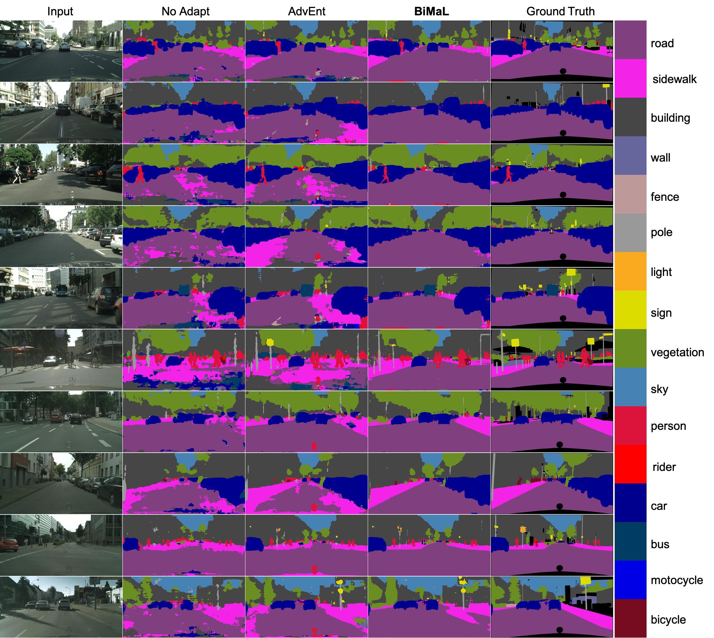
Figure 6: Qualitative results of the SYNTHIA $\to$ Cityscapes experiment. Columns 1 and 5 are the input and corresponding ground truth. Columns 2, 3 and 4 are the results of the model without adaptation, AdvEnt [54], and our method.

5.4 Comparisons with SOTA Methods

We present the experimental results of the proposed approach in comparison to other strong baselines. Comparative experiments are conducted on three benchmarks: i.e. SYNTHIA $to$ Cityscapes, GTA5 $to$ Cityscapes, and SYNTHIA $to$ Vistas. In all three benchmarks, our method consistently achieves the SOTA semantic segmentation performance in term of “mean Intersection over Union” (mIoU).

SYNTHIA $to$ Cityscapes. Table 2 presents the semantic performance (mIoU) on the 16 classes of the Cityscape validation set. Our proposed method achieves better accuracy than the prior methods, i.e. $46.2\%$ higher than DADA [55] by $3.6\%$. Considering per-class results, our method significantly improves the results on classes of ‘sidewalk’ ($51.5\%$), ‘car’ ($85.7\%$), and ‘bus’ ($44.5\%$). We also report the results on a 13-class subset where our proposed method also achieves the State-of-the-Art performance.

GTA5 $to$ Cityscapes. Table 3 shows the mIoU of 19 classes of Cityscapes on the validation set. Our approach gains mIoU of $47.3\%$ that is state-of-the-art performance compared to the prior methods. Analysing per-class results, our method gains the improvement on most classes. In particular, the results on classes of ‘terrain’ (+$10.0\%$), ‘truck’ ($+9.1\%$), ‘bus’ ($+8.0\%$), ‘motorbike’ ($+5.6\%$) demonstrate significant improvements compared to AdvEnt. For other classes, the proposed method gains moderate improvements, compared to prior SOTA methods.

Table 4: Semantic segmentation performance mIoU (%) on Vistas testing set of different models trained on SYNTHIA. (const. denotes for construction)

SYNTHIA $\to$ Vistas (7 classes)
Models	flat	const.	object	nature	sky	human	vehicle	mIoU
SPIGAN-no-PI [25]	53.0	30.8	3.6	14.6	53.0	5.8	26.9	26.8
SPIGAN [25]	74.1	47.1	6.8	43.3	83.7	11.2	42.2	44.1
AdvEnt [54]	86.9	58.8	30.5	74.1	85.1	48.3	72.5	65.2
DADA [55]	86.7	62.1	34.9	75.9	88.6	51.1	73.8	67.6
Our BiMaL	87.6	61.6	35.3	77.5	87.8	53.3	75.6	68.4

SYNTHIA $to$ Vistas. Table 4 reports the mIoU on 7 classes of the Vistas testing set. Our approach gains an mIoU of $67.2\%$ which is the SOTA performance compared to prior methods. Moreover, our method also gains moderate improvements in per-class accuracy.

Qualitative Results. Figure 6 illustrates the qualitative results of the SYNTHIA $to$ Cityscapces experiment. Our method gives the better qualitative results compared to a model trained on the source domain and AdvEnt [54]. Our method can model well the structure of an image. In particular, our results have a clear border between ‘road’ and ‘sidewalk’. Meanwhile, the results of model trained on source only and AdvEnt have an unclear border between ‘road’ and ‘sidewalk’. Overall, our qualitative semantic segmentation results are sharper than the results of AdvEnt.

6 Conclusions

This paper has presented a new Bijective Maximum Likelihood approach to domain adaptation in semantic scene segmentation. Compared to Adversarial Entropy Minimization loss, it is a more generalized form and can work without any assumption about pixel independence. In addition, a new Unaligned Domain Score metric has been also introduced to measure the efficiency of a segmentation model on a new target domain in the unsupervised manner. Through intensive experiments on three different datasets, i.e. SYNTHIA $to$ Cityscapes, GTA $to$ Cityscapes, and SYNTHIA $to$ Vistas, we achieve SOTA performance compared to prior methods. Specifically, our semantic segmentation accuracy on these three benchmarks are $46.2\%$, $47.3\%$, and $68.4\%$, respectively. The future direction of this work is to solve challenging cases coming from the differences in “segmentation structures” between source and target domains such as left- and right-hand traffic.

Acknowledgement

This work is supported by NSF Data Science, Data Analytics that are Robust and Trusted (DART), Chancellor’s Innovation Fund, UAF and NSF Small Business Grant.

References

- [1] Léon Bottou. Large-scale machine learning with stochastic gradient descent. In COMPSTAT. 2010.
- [2] Lin Chen, Wen Li, and Dong Xu. Recognizing RGB images by learning from RGB-D data. In CVPR, 2014.
- [3] Liang-Chieh Chen, George Papandreou, Iasonas Kokkinos, Kevin Murphy, and Alan L Yuille. Deeplab: Semantic image segmentation with deep convolutional nets, atrous convolution, and fully connected CRFs. TPAMI, 2018.
- [4] Minghao Chen, Hongyang Xue, and Deng Cai. Domain adaptation for semantic segmentation with maximum squares loss. In ICCV, 2019.
- [5] Yuhua Chen, Wen Li, and Luc Van Gool. Road: Reality oriented adaptation for semantic segmentation of urban scenes. In CVPR, 2018.
- [6] Yi-Hsin Chen, Wei-Yu Chen, Yu-Ting Chen, Bo-Cheng Tsai, Yu-Chiang Frank Wang, and Min Sun. No more discrimination: Cross city adaptation of road scene segmenters. In ICCV, 2017.
- [7] Marius Cordts, Mohamed Omran, Sebastian Ramos, Timo Rehfeld, Markus Enzweiler, Rodrigo Benenson, Uwe Franke, Stefan Roth, and Bernt Schiele. The Cityscapes dataset for semantic urban scene understanding. In CVPR, 2016.
- [8] Laurent Dinh, David Krueger, and Yoshua Bengio. Nice: Non-linear independent components estimation, 2015.
- [9] Laurent Dinh, Jascha Sohl-Dickstein, and Samy Bengio. Density estimation using real nvp, 2017.
- [10] Chi Nhan Duong, Khoa Luu, Kha Gia Quach, and Tien D. Bui. Longitudinal face modeling via temporal deep restricted boltzmann machines. In CVPR, 2016.
- [11] Chi Nhan Duong, Khoa Luu, Kha Gia Quach, and Tien D. Bui. Deep appearance models: A deep boltzmann machine approach for face modeling. IJCV, 2019.
- [12] Chi Nhan Duong, Khoa Luu, Kha Gia Quach, and Ngan Le. Shrinkteanet: Million-scale lightweight face recognition via shrinking teacher-student networks. arXiv:1905.10620, 2019.
- [13] Chi Nhan Duong, Khoa Luu, Kha Gia Quach, Nghia Nguyen, Eric Patterson, Tien D. Bui, and Ngan Le. Automatic face aging in videos via deep reinforcement learning. In CVPR, 2019.
- [14] Chi Nhan Duong, Kha Gia Quach, Khoa Luu, T Hoang Ngan Le, Marios Savvides, and Tien D Bui. Learning from longitudinal face demonstration—where tractable deep modeling meets inverse reinforcement learning. IJCV, 2019.
- [15] Chi Nhan Duong, Thanh-Dat Truong, Khoa Luu, Kha Gia Quach, Hung Bui, and Kaushik Roy. Vec2face: Unveil human faces from their blackbox features in face recognition. In CVPR, 2020.
- [16] Yaroslav Ganin and Victor Lempitsky. Unsupervised domain adaptation by backpropagation. In ICML, 2015.
- [17] Yves Grandvalet and Yoshua Bengio. Semi-supervised learning by entropy minimization. In NIPS, 2005.
- [18] Kaiming He, Xiangyu Zhang, Shaoqing Ren, and Jian Sun. Deep residual learning for image recognition. In CVPR, 2016.
- [19] Judy Hoffman, Saurabh Gupta, and Trevor Darrell. Learning with side information through modality hallucination. In CVPR, 2016.
- [20] Judy Hoffman, Eric Tzeng, Taesung Park, Jun-Yan Zhu, Phillip Isola, Kate Saenko, Alexei Efros, and Trevor Darrell. CyCADA: Cycle-consistent adversarial domain adaptation. In ICML, 2018.
- [21] Judy Hoffman, Dequan Wang, Fisher Yu, and Trevor Darrell. FCNs in the wild: Pixel-level adversarial and constraint-based adaptation. arXiv:1612.02649, 2016.
- [22] Weixiang Hong, Zhenzhen Wang, Ming Yang, and Junsong Yuan. Conditional generative adversarial network for structured domain adaptation. In CVPR, 2018.
- [23] Durk P Kingma and Prafulla Dhariwal. Glow: Generative flow with invertible 1x1 convolutions. In S. Bengio, H. Wallach, H. Larochelle, K. Grauman, N. Cesa-Bianchi, and R. Garnett, editors, NIPS, 2018.
- [24] T. Hoang Ngan Le, Kha Gia Quach, Khoa Luu, Chi Nhan Duong, and Marios Savvides. Reformulating level sets as deep recurrent neural network approach to semantic segmentation. TIP, 2018.
- [25] Kuan-Hui Lee, German Ros, Jie Li, and Adrien Gaidon. SPIGAN: Privileged adversarial learning from simulation. In ICLR, 2019.
- [26] Guangrui Li, Guoliang Kang, Wu Liu, Yunchao Wei, and Yi Yang. Content-consistent matching for domain adaptive semantic segmentation. In ECCV, 2020.
- [27] Wen Li, Li Niu, and Dong Xu. Exploiting privileged information from web data for image categorization. In ECCV, 2014.
- [28] Xinzhe Li, Qianru Sun, Yaoyao Liu, Qin Zhou, Shibao Zheng, Tat-Seng Chua, and Bernt Schiele. Learning to self-train for semi-supervised few-shot classification. In NeurIPS, 2019.
- [29] Mingsheng Long, Yue Cao, Jianmin Wang, and Michael I Jordan. Learning transferable features with deep adaptation networks. In ICML, 2015.
- [30] David Lopez-Paz, Léon Bottou, Bernhard Schölkopf, and Vladimir Vapnik. Unifying distillation and privileged information. In ICLR, 2016.
- [31] Yawei Luo, Liang Zheng, Tao Guan, Junqing Yu, and Yi Yang. Taking a closer look at domain shift: Category-level adversaries for semantics consistent domain adaptation. arXiv:1809.09478, 2019.
- [32] K. Luu, T. D. Bui, K. Ricanek Jr., and C. Y. Suen. Age estimation using active appearance models and support vector machine regression. In BTAS, 2009.
- [33] K. Luu, T. D. Bui, and C. Y. Suen. Kernel spectral regression of perceived age from hybrid facial features. In FG, 2011.
- [34] K. Luu, K. Ricanek Jr., T. D. Bui, and C. Y. Suen. The familial face database: A longitudinal study of family-based growth and development on face recognition. In ROBUST, 2008.
- [35] K. Luu, K. Seshadri, M. Savvides, T. D. Bui, and C. Y. Suen. Contourlet appearance model for facial age estimation. In IJCB, 2011.
- [36] Taylor Mordan, Nicolas Thome, Gilles Henaff, and Matthieu Cord. Revisiting multi-task learning with rock: a deep residual auxiliary block for visual detection. In NIPS, 2018.
- [37] Zak Murez, Soheil Kolouri, David Kriegman, Ravi Ramamoorthi, and Kyungnam Kim. Image to image translation for domain adaptation. In CVPR, 2018.
- [38] Gerhard Neuhold, Tobias Ollmann, Samuel Rota Bulò, and Peter Kontschieder. The mapillary vistas dataset for semantic understanding of street scenes. In ICCV, 2017.
- [39] Chi Nhan Duong, Kha Gia Quach, Khoa Luu, Ngan Le, and Marios Savvides. Temporal non-volume preserving approach to facial age-progression and age-invariant face recognition. In ICCV, Oct 2017.
- [40] Fei Pan, Inkyu Shin, Francois Rameau, Seokju Lee, and In So Kweon. Unsupervised intra-domain adaptation for semantic segmentation through self-supervision. In CVPR, 2020.
- [41] Adam Paszke, Sam Gross, Francisco Massa, Adam Lerer, James Bradbury, Gregory Chanan, Trevor Killeen, Zeming Lin, Natalia Gimelshein, Luca Antiga, Alban Desmaison, Andreas Köpf, Edward Yang, Zach DeVito, Martin Raison, Alykhan Tejani, Sasank Chilamkurthy, Benoit Steiner, Lu Fang, Junjie Bai, and Soumith Chintala. Pytorch: An imperative style, high-performance deep learning library, 2019.
- [42] Stephan R. Richter, Vibhav Vineet, Stefan Roth, and Vladlen Koltun. Playing for data: Ground truth from computer games. In ECCV, 2016.
- [43] German Ros, Laura Sellart, Joanna Materzynska, David Vazquez, and Antonio M. Lopez. The SYNTHIA dataset: A large collection of synthetic images for semantic segmentation of urban scenes. In CVPR, 2016.
- [44] Christos Sakaridis, Dengxin Dai, Simon Hecker, and Luc Van Gool. Model adaptation with synthetic and real data for semantic dense foggy scene understanding. In ECCV, 2018.
- [45] Nikolaos Sarafianos, Michalis Vrigkas, and Ioannis A Kakadiaris. Adaptive SVM+: Learning with privileged information for domain adaptation. In ICCV, 2017.
- [46] Viktoriia Sharmanska, Novi Quadrianto, and Christoph H. Lampert. Learning to rank using privileged information. In ICCV, 2013.
- [47] Jost Tobias Springenberg. Unsupervised and semi-supervised learning with categorical generative adversarial networks. ICLR, 2016.
- [48] Thanh-Dat Truong, Chi Nhan Duong, Khoa Luu, Minh-Triet Tran, and Ngan Le. Domain generalization via universal non-volume preserving approach. In CRV, 2020.
- [49] Thanh-Dat Truong, Chi Nhan Duong, Minh-Triet Tran, Ngan Le, and Khoa Luu. Fast flow reconstruction via robust invertible n × n convolution. Future Internet, 2021.
- [50] Yi-Hsuan Tsai, Wei-Chih Hung, Samuel Schulter, Kihyuk Sohn, Ming-Hsuan Yang, and Manmohan Chandraker. Learning to adapt structured output space for semantic segmentation. In CVPR, 2018.
- [51] Yi-Hsuan Tsai, Kihyuk Sohn, Samuel Schulter, and Manmohan Chandraker. Domain adaptation for structured output via discriminative representations. arXiv:1901.05427, 2019.
- [52] Eric Tzeng, Judy Hoffman, Kate Saenko, and Trevor Darrell. Adversarial discriminative domain adaptation. In CVPR, 2017.
- [53] Vladimir Vapnik and Akshay Vashist. A new learning paradigm: Learning using privileged information. Neural networks, 2009.
- [54] Tuan-Hung Vu, Himalaya Jain, Maxime Bucher, Matthieu Cord, and Patrick Pérez. Advent: Adversarial entropy minimization for domain adaptation in semantic segmentation. In CVPR, 2019.
- [55] Tuan-Hung Vu, Himalaya Jain, Maxime Bucher, Mathieu Cord, and Patrick Pérez. Dada: Depth-aware domain adaptation in semantic segmentation. In ICCV, 2019.
- [56] Zuxuan Wu, Xintong Han, Yen-Liang Lin, Mustafa Gokhan Uzunbas, Tom Goldstein, Ser Nam Lim, and Larry S. Davis. DCAN: Dual channel-wise alignment networks for unsupervised scene adaptation. In ECCV, 2018.
- [57] Qiming Zhang, Jing Zhang, Wei Liu, and Dacheng Tao. Category anchor-guided unsupervised domain adaptation for semantic segmentation. In NIPS, 2019.
- [58] Jun-Yan Zhu, Taesung Park, Phillip Isola, and Alexei A Efros. Unpaired image-to-image translation using cycle-consistent adversarial networks. In ICCV, 2017.
- [59] Xinge Zhu, Hui Zhou, Ceyuan Yang, Jianping Shi, and Dahua Lin. Penalizing top performers: Conservative loss for semantic segmentation adaptation. In ECCV, 2018.
- [60] Yang Zou, Zhiding Yu, BVK Vijaya Kumar, and Jinsong Wang. Unsupervised domain adaptation for semantic segmentation via class-balanced self-training. In ECCV, 2018.