Loss of Antibunching

Abstract

We describe some of the main external mechanisms that lead to a loss of antibunching, i.e., that spoil the character of a given quantum light to deliver its photons separated the ones from the others. Namely, we consider contamination by noise, a time jitter in the photon detection and the effect of frequency filtering (or detection with finite bandwidth). The emission from a two-level system under both incoherent and coherent driving is taken as a particular case of special interest. The coherent case is further separated into its vanishing (Heitler) and high (Mollow) driving regimes. We provide analytical solutions which, in the case of filtering, unveil an unsuspected structure in the transitions from perfect antibunching to thermal (incoherent case) or uncorrelated (coherent case) emission. The experimental observations of these basic and fundamental transitions would provide another compelling evidence of the correctness and importance of the theory of frequency-resolved photon correlations.

I Introduction

Antibunching [1] describes one of the most popular type of quantum light, the one for which photons get separated from each other and avoid the opposite bunching tendency of bosons to appear clumped together [2]. Through its observation by Kimble in 1977 [3], it provided the first direct evidence of quantization of the light field, that is to say, the first observation, albeit indirect, of photons. Antibunched light is also of considerable importance for quantum applications, for instance to feed quantum gates or for the already commercialized quantum cryptography, in which case one seeks the ultimate antibunching where transform-limited photons [4] are never detected more than one at a time. This would provide the ultimate antibunching. This is an asymptotic race, however, as perfect antibunching has still not been achieved and some residual multiple-photon emission has always accompanied the most crafted setups. In principle, since we are dealing with a quantized property, with a gap separating its value (one photon) from its neighbours (vacuum and two or more photons), there is no a priori reason why one could not observe perfect antibunching, just as one does observe perfect conductivity from a superconductor or perfect flow from a superfluid. In all these cases, there are experimental limitations, inaccuracy of measurements, finite times and energy involved, and yet, one can show that the measurement of resistance is compatible with a mathematical zero in a superconductor, where experiments with superconducting coils have demonstrated current flow persisting for years without degradation, points to a current lifetime of at least 100,000 years and with theoretical estimates for the lifetime of a persistent current to exceed the lifetime of the universe [5]. This is in this sense that one can speak of the resistance becoming “truly zero” in a superconductor. Instead, when it comes to the more basic problem of detecting a single photon, one finds instead deviation from uncorrelated light of at best (to the best of our knowledge) $7.5\times 10^{-5}$ [6] and $9.5\times 10^{-5}$ [7] which are, furthermore, sensibly better than most values reported in an ample literature (which cannot be browsed completely even if we narrow it down to recent reports below $10^{-2}$ [8, 9, 10, 11, 12, 13, 14, 15, 16, 17, 6, 18, 7, 19, 20], see Ref. [21] for a recent review.) The record-value antibunching [6, 7] were significantly improved by counteracting re-excitations of the two-level system by implementing improved two-photon excitation schemes (In Ref. [22], we have also discussed how exciting a 2LS with quantum light indeed improves its single-photon characteristics). But even with this newly added trick to suppress multiphoton emission, the perfect antibunching of an exact zero—or no-coincidence at all however long the experiment is run—is still out of reach. In this text, we discuss mechanisms that leads to a loss of antibunching, regardless of the source of light itself which can, indeed, be perfectly antibunched. We cover both technical (noise, time-jitter) as well as fundamental reasons (linked to photon-detection).

II Definition of antibunching

The definition of antibunching requires some discussion, as it varies throughout times and authors [23] and is commonly confused for another one (subpoissonian statistics). At the heart of every definition one finds Glauber’s theory of optical coherence [24], that introduces correlation functions $g^{(n)}$ for the $n^{\mathrm{th}}$-order coherence as

$$g^{(n)}(t_{1},\cdots,t_{n})\equiv\\ \frac{\langle{a^{\dagger}}(t_{1}){a^{\dagger}}(t_{2})\cdots{a^{\dagger}}(t_{n})a(t_{n})\cdots a(t_{2})a(t_{1})\rangle}{\langle{a^{\dagger}}(t_{1})a(t_{1})\rangle\langle{a^{\dagger}}(t_{2})a(t_{2})\rangle\cdots\langle{a^{\dagger}}(t_{n})a(t_{n})\rangle}\,,$$ (1)

where we have assumed that the times $t_{k}$ are in increasing order, i.e., $t_{1}<t_{2}<\cdots<t_{n}$, and we have assumed a single bosonic mode $a$, which is the best way to root our discussion at its most fundamental level, since involving a continuum from the start should eventually bring us to the same results. At the two photons level, that of more common occurence, Eq. (1) reads

$$g^{(2)}(t_{1},t_{2})={\langle{a^{\dagger}}(t_{1}){a^{\dagger}}(t_{2})a(t_{2})a(t_{1})\rangle\over\langle({a^{\dagger}}a)(t_{1})\rangle\langle({a^{\dagger}}a)(t_{1})\rangle}$$ (2)

and if dealing with a steady state, so that only the time difference $\tau\equiv t_{2}-t_{1}$ matters:

$$g^{(2)}(\tau)={\langle{a^{\dagger}}{a^{\dagger}}(\tau)a(\tau)a\rangle\over\langle{a^{\dagger}}a\rangle^{2}}\,.$$ (3)

At zero time delay $\tau=0$, Eq. (3) further simplifies to

$$g^{(2)}(0)={\langle{a^{\dagger 2}}a^{2}\rangle\over\langle{a^{\dagger}}a\rangle^{2}}\,,$$ (4)

and the application of Eq. (4) on a density matrix $\rho$ yields the two-photon coincidences $g^{(2)}(0)$ in terms of the probabilities $p(n)\equiv\left\langle n\right|\rho\left|n\right\rangle$ as:

$$g^{(2)}(0)={\sum_{n=0}^{\infty}n(n-1)p(n)\over(\sum_{n=0}^{\infty}np(n))^{2}}\,.$$ (5)

Antibunching is nowadays commonly defined by the condition [25, 26]:

$$g^{(2)}(0)<g^{(2)}(\tau)\hbox{ for all $0\leq\tau<\tau_{\mathrm{max}}$}\,,$$ (6)

where $\tau_{\mathrm{max}}$ can be infinite. Since for time delays long enough, photons are uncorrelated, which means, by definition, that the numerator in Eq. (3) factorizes in the form of the denominator, i.e., $\lim_{\tau\rightarrow\infty}g^{(2)}(\tau)=1$, then a popular understanding of antibunching reads

$$g^{(2)}(0)<1\,.$$ (7)

This is inaccurate at best since Eqs. (6) and (7) are logically independent, i.e., none implies the other, although they are strongly related to each others [27]. This point has been made by Zou and Mandel [28]. A proper name for Eq. (7) is sub-Poisson light [23] (other denominations can be found such as “photon-number-squeezed light” [23]). Such discussions truely become important for particular, and often, odd cases such as antibunching of super-Poissonian light. In this text, we will focus on the simplest case that is also that of greatest (today’s) interest of sub-Poissonian antibunched light, so such precautions in the terminology will not be entirely necessary. By antibunching, we shall thus understand the tendency of emitting single photons, as is often the case in the literature anyway. Note that our formalisms and results could nevertheless be applied to all types of photon correlations (superbunching, etc.) but we will focus presently on antibunching.

III Measurement of antibunching

The typical setup for measuring antibunching experimentally is that designed by Hanbury Brown [29] to implement an intensity interferometer following his naked-eye observation of radar correlations in the early days of its elaboration. While initially designed for interferometry in radio-astronomy [30], its application to visible light was quickly understood as involving photon correlations at the single-particle level, which initially caused much controversy but was quickly confirmed experimentally [31] (the denomination of “coherent” for the beams of light in Ref. [31] predates Glauber’s theory of optical coherence and refers to monochromatic thermal light). The theory of the effect by Twiss gives to the setup its famed name of Hanbury Brown–Twiss (HBT) interferometer. While designed for bunching—the natural tendency of bosons which symmetric wavefunctions tend to clutter together—the same setup is apt to measure all types of photon correlations, including antibunching, as had been readily predicted [32, 33]. The HBT setup consists in a beam-splitter followed by two detectors in each branch which are temporally correlated. In practice, the first detector that records a click starts a time-counter while the other detector stops it and a normalized histogram of the time differences $\tau$ between the successive photons thus reconstructs the second-order coherence function $g^{(2)}(\tau)$. It is also known as a photon-coincidence measurement. The critical elements that affect the quantum correlations in this setup are the detectors, which are typically APDs (Avalanche photodiodes) [34]. The most frequently used detectors for detection of low-intensity light are photomultiplier tubes (PMTs), but their quantum efficiency is small (smaller than 50%). For this reason APDs are used, which have an additional gain mechanism, the ‘avalanch effect’. With the APDs, a stable gain on the order of $10^{2}$ to $10^{3}$ can be achieved, which is still too low to detect single photons. For this purpose, the APDs must be used in the ‘Geiger mode’ [35]. These single-photon avalanche photodiodes (SPADs) have a high detection efficiency and low dark count rates, but they are slow and with a big timming jitter (typically $300-400$ ps, with low values of $35$ ps [36]). To multiply the signal, they use semiconductor materials. Depending on these materials, the APDs operate in different frequency windows between $550$ and $1550$ nm. Another source of noise characteristic of APDs is the afterpulsing, which can limit the count rate [37].

New methods have emerged to measure photon correlations, in particular one that relies on a direct observation of the photon streams as measured by a streak camera [38]. The detected photons are first transformed into photoelectrons by means of a photocathode. These new photoelectrons are deflected vertically to different pixels on the detector as a function of time. Thanks to this shift, the vertical position on the detector defines the time of arrival of the photon. Streak cameras have low detection efficiency but allow for a resolution of the order of the ps. They operate in frequency windows of $300-1700$ nm, depending on the material used for the photocathode. One advantage of a streak camera setup in a cw regime is that it provides the raw result with no need for post-processing or normalization. Namely, the condition $g^{(2)}(\tau\to\infty)=1$ which is used to normalize the signal in the case of an HBT measurement, should be automatically verified with the streak setup. Failure to be the case should point at some problem in the detection, e.g., non-stationarity of the signal [39]. This also allows to compute higher-order photon correlations, which can also be achieved with other emerging techniques such as transition edge sensors set up to direclty resolve the number of detected photons [40].

With this brief overview of some of the main methods to measure antibunching, one gets a feeling of the mechanisms that lead to its loss and that we will model theoretically in the following. These include, basically, external noise and time uncertainty in the detection. The latter can be due to a jitter, meaning that a fluctuation or scrambling of the arrival time due to the detector, or at a more fundamental level, be linked to the time-energy uncertainty which is inherent even to ideal detectors. We will cover both mechanisms. Interestingly, photon-losses, which constitute an important limitation of all schemes of photon detections, are not detrimental for the measurement of antibunching. This merely dims the signal, but preserves its statistics. Although only a coherent signal can pass linear optical element without being distorted, and that subpoissonian or superpoissonian signals get closer to Poissonian distributions, e.g., by passing through beam-splitters [41], this, however, refers to the noise of the signal rather than to its statistics. A well ordered stream of single photons would appear less ordered in the presence of losses, but this would in no way lead to spurious coincidences. Such a closeness to a Poissonian distribution is typically measured by the Fano factor, which relates the width of the input distribution to the expected one for a Poissonian distribution with the same average number as $F=(\langle n^{2}\rangle-\langle n\rangle^{2})/\langle n\rangle$. Therefore, as the Fano factor can grow linearly from 0, corresponding to a Number-state distribution, to 1, corresponding to a Poisson distribution, as the probability to loose any one photon of the input beam is increased, the statistics as measured by $g^{(2)}(0)$ remains constant, equal to that of the ideal signal. This is clear on physical grounds since removing photons to an antibunched signal cannot create bunching. What is spoiled is the signal, which can however be compensated by longer integration times. The loss is therefore in quantity, not in quality. This features makes the lossy setups, including the HBT one, able to measure antibunching as it does not matter that strictly successive photons be recorded, $g^{(2)}(\tau)$ being a density probability for any two photons to be separated by the interval $\tau$, regardless of whether other photons are present in between or not. In fact, a histogram of exactly successive photons would fail to produce the uncorrelated plateau at long $\tau$. We can therefore already strike out one of the main difficulties encountered in the experiment and focus on the other above-cited mechanisms. Before turning to them in detail, we first review the antibunching from the source we shall use to illustrate the general theory, which is of great interest regardless, being the most fundamental and widespread type of single-photon source.

IV Examples of antibunching

The two-level system (2LS) is the paradigmatic source of single photons. When the emission occurs with the system relaxing from its excited to its ground state, and since it takes a finite amount of time for the 2LS to be re-excited, together with the impossibility to host more than one excitation at a time, two photons can never be emitted simultaneously. This is at least the basic picture which one can form and that applies in the simplest cases of incoherent excitation as well as strong coherent excitation. Under weak coherent excitation, on the other hand, subtle interferences at the multi-photon level also produce antibunching but with a distinct physical origin [42]. In the remaining of the text we will work with these three cases: i) incoherent and ii) coherent excitation, the latter being further separated into its weak (Heitler) and high (Mollow) regimes.

IV.1 Incoherent excitation

The Hamiltonian of an incoherently driven 2LS is simply its free energy, namely

$$H_{\sigma}=\omega_{\sigma}{\sigma^{\dagger}}\sigma\,,$$ (8)

where the 2LS is described through the annihilation operator $\sigma$, which satisfies the algebra of pseudo-spins, and $\omega_{\sigma}$ is the natural frequency of the 2LS. Both the excitation and decay of the 2LS is taken into account by turning to a master equation (we use $\hbar=1$ along the paper)

$$\partial_{t}\rho=i[\rho,H]+\sum_{k}\mathcal{L}_{c_{k}}\rho\,,$$ (9)

with the Lindblad terms $\mathcal{L}_{\sigma^{\dagger}}\rho=(P_{\sigma}/2)(2{\sigma^{\dagger}}\rho\sigma-\sigma{\sigma^{\dagger}}\rho-\rho\sigma{\sigma^{\dagger}})$, where $P_{\sigma}$ is the rate of excitation and $\mathcal{L}{\sigma}\rho=(\gamma_{\sigma}/2)(2{\sigma}\rho{\sigma^{\dagger}}-{\sigma^{\dagger}}{\sigma}\rho-\rho{\sigma^{\dagger}}{\sigma})$, where $\gamma_{\sigma}$ is the decay rate. It is then a simple algebraic procedure to obtain the second-order correlations of a 2LS under incoherent driving as

$$g^{(2)}_{\sigma,P_{\sigma}}(\tau)=1-e^{-\Gamma_{\sigma}\tau}\,,$$ (10)

in terms of the effective decay rate $\Gamma_{\sigma}\equiv\gamma_{\sigma}+P_{\sigma}$ that causes the power-broadening of the emission spectrum.

IV.2 Coherent excitation

The counterpart of the previous section but for coherent excitation is described by supplementing the master equation (9) with the Hamiltonian

$$H_{\sigma}=\omega_{\sigma}{\sigma^{\dagger}}\sigma+\Omega_{\sigma}(\sigma e^{i\omega_{\mathrm{L}}t}+{\sigma^{\dagger}}e^{-i\omega_{\mathrm{L}}t})\,,$$ (11)

where $\Omega_{\sigma}$ is the intensity at which the 2LS is driven by a laser, which emits photons at a frequency $\omega_{\mathrm{L}}$. The temporal dependence of the Hamiltonian in Eq. (11) is removed by making a Dirac transformation, leaving the contribution from the free energy of the 2LS and of the detector proportional to the detuning between the laser and their natural frequencies, namely, $\Delta_{c}\equiv(\omega_{c}-\omega_{\mathrm{L}})$ for $c=\sigma,a$.

The same techniques applied to this variation of the problem provide the correlations for the 2LS under coherent excitation as

$$g^{(2)}_{\sigma,\Omega}(\tau)=1-e^{-3\gamma_{\sigma}\tau/4}\left[\cos\left(\frac{\gamma_{\mathrm{M}}\tau}{4}\right)+\frac{3\gamma_{\sigma}}{\gamma_{\mathrm{M}}}\sin\left(\frac{\gamma_{\mathrm{M}}\tau}{4}\right)\right]\,,$$ (12)

where $\gamma_{\mathrm{M}}\equiv\sqrt{\gamma_{\sigma}^{2}-(8\Omega_{\sigma})^{2}}$ (‘M’ is for “Mollow”) and $\Omega_{\sigma}$ is the intensity of the driving laser. This more involved expression follows from the two regimes of low and high driving. In the Heitler regime [43], where the rate of excitation is much weaker than the decay rate of the 2LS, the correlations simplify to

$$g_{\sigma,\Omega\rightarrow 0}^{(2)}(\tau)=\left(1-e^{-\gamma_{\sigma}\tau/2}\right)^{2}\,,$$ (13)

and in the limit of large driving, the correlations are strongly oscillating between the envelopes

$$g_{\sigma,\Omega\rightarrow\infty}^{(2)}(\tau)=1\pm e^{-3\gamma_{\sigma}\tau/4}\,,$$ (14)

that decay from 0 and 2 respectively to 1. Note also that the expressions in Eqs. (10), (12–14) are auto-correlations, and as such they are symmetric functions, namely $g_{\sigma}^{(2)}(-\tau)=g^{(2)}_{\sigma}(\tau)$.

Already, we have more than enough material to study from this basic emitter the highly-nontrivial physics of loss of antibunching, and we will focus the rest of our discussion on this case. Other antibunched sources would either behave similarly and/or could be studied following a similar approach.

V Loss of antibunching by noise contamination

A first obvious and simple way that antibunching can be lost is due to the signal being perturbed by noise. Dark counts, for instance, which correspond to photon-detection even in absence of light (whence the name) [44], clearly spoil antibunching, since the extra photon can arrive simultaneously with a signal photon that was supposed to be detected in isolation. Also, in some cases, the laser driving the system can directly inject a spurious fraction of photons into the detectors [45]. All these photons that are uncorrelated with the source cause a random noise, or shot noise, which (usually) spoils antibunching (shoit noise usually assume Poissonian statistics of the noise).

If we call $I(t)$ the instantaneous photon intensity from the source (signal) and $I^{\prime}(t)$ that of the randomly added photons (noise), the total final intensity is given by:

$$I^{*}(t)=I^{\prime}(t)+I(t)\,,$$ (15)

and the photon statistics of the total signal is given by

$$g^{*(2)}(\tau)=\frac{\langle{:}I^{*}(t)I^{*}(t+\tau){:}\rangle}{\langle I^{*}(t)\rangle^{2}}\,,$$ (16)

where ${:}\cdots{:}$ normal-orders the operators so that they appear in the form of Eq. (2). Since signal and noise are uncorrelated $\langle{:}I(t)I^{\prime}(t^{\prime}){:}\rangle=\langle I(t)\rangle\langle I^{\prime}(t^{\prime})\rangle$ for all $t$, $t^{\prime}$and also introducing $\xi$ the noise to signal ratio, i.e., $\xi\equiv\langle I^{\prime}(t)\rangle/\langle I(t)\rangle$, one can get a simple expression that relates the photon statistics of the signal contaminated by the noise with statistics $g^{\prime(2)}(\tau)\equiv\langle{:}I^{\prime}(t)I^{\prime}(t+\tau){:}\rangle/{\langle I^{\prime}(t)\rangle^{2}}$ to that of the original signal $g^{(2)}(\tau)$ as

$$g^{*(2)}(\tau)=\frac{1}{(1+\xi)^{2}}\left(g^{(2)}(\tau)+\xi^{2}g^{\prime(2)}(\tau)+2\xi\right)\,.$$ (17)

If the noise has no correlation, $g^{\prime(2)}(\tau)=1$ for all $\tau$ and for perfect antibunching with $g^{(2)}(0)=0$, the loss of antibunching $\xi(2+\xi)/(1+\xi)^{2}$ requires a noise-to-signal ratio of $\sqrt{2}-1\approx 42\%$ to spoil it to 0.5 and even when there is twice as much noise as perfectly antibunched signal, the resulting antibunching of $8/9\approx 0.89$ is still comfortably observed. The random noise tends to flatten the correlations to that of an uncorrelated (coherent) signal with $g^{*(2)}(\tau)=1$ everywhere, in a way that shifts the curves to one, without transforming bunching into antibunching or vice versa [46]. It also has no effect on the coherence time (the time necessary for the correlation to converge to one is independent of the percentage of noise). Thermal noise, not surprisingly, is more detrimental to antibunching, with $\xi=1/3$ to spoil perfect antibunching to 0.5 and when noise and signal are equal in intensity, then $g^{*(2)}(0)=1$ with super-Poissonian statistics for higher $\xi$. Depending on the coherence time of the thermal light, $g^{*(2)}(\tau)$ is either bunched or antibunched in the sense of decreasing or increasing correlations in time. If the noise itself is antibunched, it cannot increase $g^{*(2)}(0)$ beyond $0.5$, which it does when $\xi=1$. Further noise reduces $g^{*(2)}(0)$ again as the original signal becomes the noise for the now dominating antibunching. In all cases, in the limit $\xi\to\infty$, $g^{*(2)}(\tau)\to g^{\prime(2)}(\tau)$ and then one observes the noise itself, so what is lost is indeed the antibunching of the signal (such as its coherence time). Finally, we commented already how a possible source of noise is from the driving laser itself. We have assumed in this discussion that noise and signal are independent and do not interfere, so that their intensity simply add in a way reminiscent of a classical pictures of photons as particles which are superimposed the ones onto the others. In this respect the normal ordering above plays no direct role and one could understand the result with classical stochastic fields $I$ which are not number-operators. It could also be the case that the admixing of the two quantum fields is done at the level of their amplitudes, in which case the description would need to be along the lines of Ref. [47] where time and operator orderings would be significant and more complex correlations could be obtained as a result.

VI Loss of antibunching by time uncertainty

We now turn to the loss of antibunching due to a time uncertainty in the detection of the photons. Such a scenario can be due to a dead-time of the detector or a jitter effect. In both cases, the result is that a photon arriving to the detector at a time $t_{0}$ is reported by the latter at some other time $t_{0}+t$, with $t$ following a probability distribution $D^{2}_{\Gamma}(t)$, to which we will refer as the “jitter” function. The parameter $\Gamma$ is the inverse of the mean jitter time, and it is also a measure of the width of the distribution. Independently of $\Gamma$, since we assume perfect detection, the jitter function must be such that

$$\int_{-\infty}^{\infty}D_{\Gamma}^{2}(t)\,dt=1\,,$$ (18)

implying that all the photons that arrive to the detector are ultimately reported. The temporal structure of the photon stream that is received by the detector is modified by the jitter function. Its effect can be formally taken into account through the physical spectrum of emission, defined as [48]

$$S_{\Gamma}^{(1)}(\omega,T)=\frac{1}{2\pi}\iint_{-\infty}^{\infty}D_{\Gamma}(T-t_{1})D_{\Gamma}(T-t_{2})\\ e^{i\omega(t_{2}-t_{1})}\langle{a^{\dagger}}(t_{1})a(t_{2})\rangle\,dt_{1}dt_{2}\,,$$ (19)

where $a$ is the annihilation operator of the field emitting the photons and $\omega$ is the frequency at which these photons are being emitted. Integrating Eq. (19) in frequency leads to the time-resolved population

$$S_{\Gamma}^{(1)}(T)=\int_{-\infty}^{\infty}D^{2}_{\Gamma}(T-t)\langle{a^{\dagger}}a\rangle(t)\,dt\,.$$ (20)

Namely, the time-resolved population of the light emitted is the convolution of the population with the jitter function. If the signal is in a steady state, then the population is independent of time, $\langle{a^{\dagger}}a\rangle=n_{a}$, and we find that the time-resolved population is equal to the total intensity, $S_{\Gamma}(T)=n_{a}$, and that the jitter does not play a role on this observation. This makes sense since in the steady state, shuffling the times at which the photons are reported does not change the mean number of detected photons per unit time.

Applying the same treatment to the intensity-intensity correlation function describes the effect of the time jitter on $g^{(2)}(\tau)$ which now persists even in the steady state. Instead of the physical spectrum, one starts in this case with the second-order correlation function resolved in time and frequency [49]:

$$S_{\Gamma_{1}\Gamma_{2}}^{(2)}(\omega_{1},T_{1};\omega_{2},T_{2})=\frac{\Gamma_{1}\Gamma_{2}}{(2\pi)^{2}}\iiiint_{-\infty}^{\infty}dt_{1}dt_{2}dt_{3}dt_{4}\\ D_{\Gamma_{1}}(T_{1}-t_{1})D_{\Gamma_{1}}(T_{1}-t_{4})D_{\Gamma_{2}}(T_{2}-t_{2})D_{\Gamma_{2}}(T_{2}-t_{3})\\ e^{i\omega_{1}(t_{4}-t_{1})}e^{i\omega_{2}(t_{3}-t_{2})}\langle\mathcal{T}_{-}[{a^{\dagger}}(t_{1}){a^{\dagger}}(t_{2})]\mathcal{T}_{+}[a(t_{3})a(t_{4})]\rangle\,.$$ (21)

where $\Gamma_{1}$ and $\Gamma_{2}$ accommodate the fact that the pair of photons can be recorded by detectors with different jitters, and where $\mathcal{T}_{\pm}$ means time-reordering of the operators so that the first time is to the far right/left, and the whole expression is time-ordered. Assuming that the uncertainty for both detectors is equal (i.e., $\Gamma_{1}=\Gamma_{2}=\Gamma$), the frequency-integrated quantity becomes:

$$S_{\Gamma}^{(2)}(T_{1};T_{2})=\iint_{-\infty}^{\infty}D^{2}_{\Gamma}(T_{1}-t_{1})D^{2}_{\Gamma}(T_{2}-t_{2})\\ \langle\mathcal{T}_{-}[{a^{\dagger}}(t_{1}){a^{\dagger}}(t_{2})]\mathcal{T}_{+}[a(t_{2})a(t_{1})]\rangle\,dt_{1}dt_{2}\,,$$ (22)

which corresponds to the intensity correlations between two branches of a split-signal that is affected by the time jitter. Time ordering of the operators leads to two integration regions, $t_{1}>t_{2}$ and $t_{2}>t_{2}$, that allows to express Eq. (22) in terms of the standard $G^{(2)}(t,x)$ of the system, letting $t=\mathrm{min}(t_{1},t_{2})$ and $x=|t_{1}-t_{2}|$:

$$S_{\Gamma}^{(2)}(T_{1};T_{2})=\\ \int_{-\infty}^{\infty}dt\int_{0}^{\infty}dx\,G^{(2)}(t,x)\left[D^{2}_{\Gamma}(T_{1}-t)D^{2}_{\Gamma}(T_{2}-t-x)\right.+{}\\ \left.{}+D^{2}_{\Gamma}(T_{1}-t-x)D^{2}_{\Gamma}(T_{2}-t)\right]\,,$$ (23)

where $0\leq x<\infty$ represents the delay between the two detected photons. The second-order correlations function of the stream of photons affected by the time jitter is then obtained by normalizing Eq. (23) with Eq. (20) as

$$g_{\Gamma}^{(2)}(T_{1};T_{2})=S_{\Gamma}^{(2)}(T_{1};T_{2})/[S_{\Gamma}^{(1)}(T_{1})S_{\Gamma}^{(1)}(T_{2})]\,.$$ (24)

In the case of a steady state, it is convenient to express the correlations as a function of the time-delay between the photon pairs (the initial time is irrelevant in this case). This provides the main result of this Section in the form of the jittered $g_{\Gamma}^{(2)}$ expression from that of the original signal as affected by the jitter function $D_{\Gamma}$:

$$g_{\Gamma}^{(2)}(\tau)=\\ \int_{0}^{\infty}g^{(2)}(\theta)\int_{-\infty}^{\infty}\left[D^{2}_{\Gamma}(-t-\theta)D^{2}_{\Gamma}(\tau-t)\right.+{}\\ \left.{}+D^{2}_{\Gamma}(-t)D^{2}_{\Gamma}(\tau-t-\theta)\,dt\right]\,d\theta\,,$$ (25)

where we have used the fact that in the steady state $S_{\Gamma}^{(1)}(T)=n_{a}$ is independent of time, and $g^{(2)}(\theta)$ is the second-order correlation of the photon stream without the time-jitter. Equation (25) is general: it holds for any $g^{(2)}(\theta)$ (as long as it is obtained in the steady state), and the particular shape of the correlations with time jitter will be given by the rightmost integral, which depends only on the jitter function.

We now consider a few particular cases for the jitter function, describing a possible physical origin in each case. The analytical expressions for the corresponding photon correlations for the emission from a two-level system (2LS) in the various regimes of excitation—which generalize the fundamental expressions (10) & (12)—can be obtained in all theses cases, but they are bulky and not enlightening per se, therefore we provide their full expression in the appendix. All the distributions have been chosen such that their variance be identical, namely, equal to $1/\Gamma^{2}$, so as to compare them usefully (the variance is a better indicator of the effect of the distribution on antibunching than the mean).

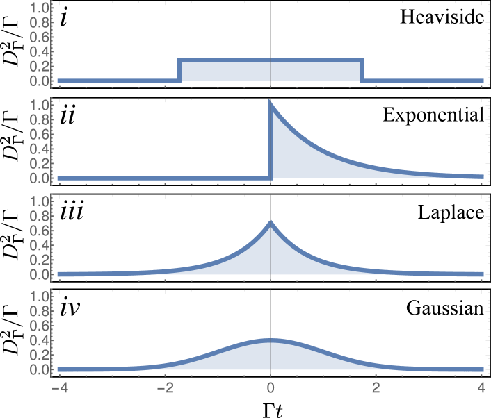
Figure 1: Jitter functions considered in this text, namely ($i$) Heaviside, Eq. (26), ($ii$) Single exponential, Eq. (27), ($iii$) Double exponential (Laplace), Eq. (28) and ($iv$) Gaussian, Eq. (29), all with the variance $1/\Gamma^{2}$. A photon from the original signal at time $0$ is replaced by one at time $t$ following the respective distributions.

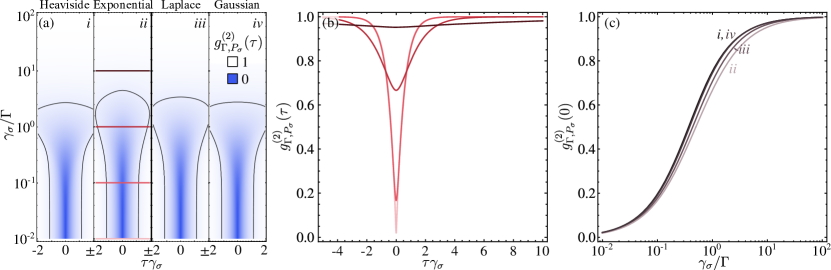
Figure 2: Photon-correlations with various types of time jitter for the incoherently driven 2LS. (a) Transition from perfect antibunching when the mean jitter time $\tau_{j}$ vanishes (corresponding to a large $\Gamma$ of the jitter functions) to uncorrelation. The progression occurs at different speeds depending on the type of jitter, namely, $i$ Heaviside, $ii$ Double exponential, $iii$ Single exponential and $iv$ Gaussian. The black contours shows the isolines $g^{(2)}_{\Gamma,P_{\sigma}}=0.9$ (b) Cuts along the lines marked in (a)$iii$ (single-exponential). (c) Zero delay correlations for the various types of jitter. All figures are for $P_{\sigma}=\gamma_{\sigma}$.

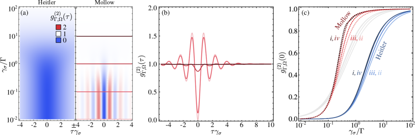
Figure 3: Photon-correlations with various types of time jitter for the coherently driven 2LS. (a) The loss of antibunching depends strongly on the regime of excitation, i.e., in the Heitler regime (left) the transition to uncorrelation requires a greater time jitter than in the Mollow triplet regime (right). The behavior with the four jitter functions follows the trend shown in Fig. 2(a), and therefore we only show the case for the single exponential. (b) Cuts along the lines marked on (a) for the Mollow triplet, showing the dampening of the correlations as the mean jitter time increases. (c) Zero delay correlations: the solid and dashed lines correspond to the 2LS driven in the Mollow and Heitler regimes, respectively. The various lines $i$–$iv$ correspond to the different jitter functions, namely, Heaviside, double exponential, single exponential and Gaussian, respectively. Figures are for $\Omega={\color[rgb]{1,0,0}??}$ in the Heitler regime and $\Omega=2\gamma_{\sigma}$ in the Mollow regime.

1. The Heaviside function describes a device that has no time resolution within a given time window, in which case, the jitter function reads

   $$\kern 21.33955ptD_{\Gamma}(t)\equiv\sqrt{\Gamma\over\sqrt{12}}\theta\left(1-{2\Gamma t\over\sqrt{12}}\right)\theta\left({1}+{2\Gamma t\over{\sqrt{12}}}\right)\,,$$ (26)

   where $\theta(t)$ is the Heaviside function, and the distribution in Eq. (26) is only nonzero in the interval $|t|<\sqrt{3}/\Gamma$ (chosen, again, so that the variance of the jitter is $1/\Gamma^{2}$). This could correspond to a streak camera which randomizes the time information within one pixel of the CCD camera [50]. The filtered correlations are given by Eq. (46) for incoherent excitation and by Eq. (48) for coherent excitation.

2. The Exponential function describes a device that is equally likely to trigger the signal at any moment that follows its excitation, with jitter function

   $$D_{\Gamma}(t)=\sqrt{\Gamma}\theta(t)e^{-\Gamma t/2}\,,$$ (27)

   where $\theta(t)$ is the Heaviside function, as shown in Fig. 1(b). This describes a wide class of devices with a memoryless dead time. The filtered correlations are given by Eq. (50) for incoherent excitation and by Eq. (51) for coherent excitation.

3. The double exponential function, also known as Laplace distribution, describes a device that has a memoryless dead time not only in its signal emission, like the previous type, but also in its excitation time, with jitter function

   $$D_{\Gamma}(t)=\sqrt{{\Gamma\over\sqrt{2}}}e^{-|t|\Gamma/\sqrt{2}}\,,$$ (28)

   shown in Fig. 1(c). It can be seen as a refinement of the two previous cases, where the variation at which the photons are reported can be both delayed or advanced according to an exponential function. The filtered correlations are given by Eq. (54) for incoherent excitation and by Eq. (55) for coherent excitation.

4. Finally, the Gaussian function describes normally-distributed fluctuations in the detection time, with jitter function

   $$D_{\Gamma}(t)=\frac{\sqrt{\Gamma}}{(2\pi)^{1/4}}e^{-(\Gamma t/2)^{2}}\,.$$ (29)

   This could be due to, e.g., the electronics involved in the detection of a photon after its arrival, or various types of noise [51]. The filtered correlations are given by Eq. (58) for incoherent excitation and by Eq. (59) for coherent excitation.

The two-photon correlations as seen by a detector with the four types of time jitters just described are shown in Fig. 2 for incoherent excitation and in Fig. 3 for coherent excitation, as follows from the analytical expressions given in the appendix.

The most striking result is that while various types of jitter result in an overall identical loss of antibunching, the robustness of the photon correlations depends on the type and the regime of driving, even though the emitter is the same (2LS), namely, the most robust photon correlations are from the coherent driving in the Heitler regime. This can be understood to some extent from the coherence time of these correlations, which is shorter than for the incoherently driven 2LS. Comparing the panels (c) in Figs. 2 and 3 (the trace of the former are reproduced in light-gray in the latter), one can see how the Mollow regime, the incoherent 2LS and finally the Heitler regime appear in order of least robust to most robust (the same amount of any type of jitter affects much more the Mollow antibunching than it does its Heitler counterpart). For very small filtering, with $\Gamma/\gamma_{\sigma}\lessapprox 0.1$, the Mollow antibunching gets more robust than the incoherent 2LS, which is very fragile to imperfect detection. It is well-known that resonant excitation yields stronger antibunching but this is attributed to the cleaner environment that is free of carriers, heating, etc. Here we find that at a fundamental level too, resonant excitation typically produces a stronger antibunching in the sense that it is more resilient to factors that spoils it. The Heaviside and Gaussian types of jitter lead to almost identical losses of antibunching, suggesting that spreading more photons has a worse effect than displacing fewer of them but farther. There is, nevertheless, a difference between the Haviside and Gaussian types of jitter in the Mollow case, since the former filters resolves the side peaks “all of a sudden”, while the Gaussian perceives them in advance, showing as well the importance of the spectral structure. This produces, when that happens, a ripple in the loss of antibunching with heaviside-type of jitter. In all cases, the single-exponential, memory-less jitter, is the one that least affects the antibunching. Since the exact, quantitative results differ only slightly from one type of jitter to the other, we show the traces for the loss of antibunching for one case only ($ii$, single-exponential) in Panels (b), where the temporal dependence also exhibits a change in the correlation time in addition to the damping of the correlations. In all cases, in the limit of large widths of the jitter noise, the correlations follow a Poisson distribution. The mean uncertainty brought to the times at which the photons are observed increases to a point where times are essentially randomized. While this is true regardless of the type of jitter, the speed of this randomization varies.

As a concluding remark, while there is, obviously, a link between the type of time uncertainty and the observed correlations, this does not follow from a mere convolution of the naked signal with the noise and involves some specifics of the dynamics (such as the regime of driving). Therefore, the original correlations cannot be recovered simply by deconvolution of the raw data, and while we do not discuss here how serious or superficial is this problem, or how it could be best compensated for, care should be exerted regarding the methods reported in the literature that seem to overlook these aspects [52, 53, 54, 55, 56, 57, 58, 59, 60, 61, 62, 63, 64, 65, 66, 67, 68, 69, 70, 71, 72, 73].

VII Loss of antibunching by frequency filtering

Antibunching is also spoiled by another reason, this time more fundamental since it is inherent to any detection process. Consider a photon counting experiment in which one not only has the information about the time of arrival, but also about the frequency (or energy) of the detected photon. In such a scenario, Heisenberg’s uncertainty principle applies: the absolute uncertainty about the frequency of the photons allows to have a perfect resolution in the time of arrival (and therefore in the time of emission) of each photon. Satisfying this condition allows to observe perfect antibunching, namely, for a 2LS, the second-order correlation functions given in Eq. (10) and Eq. (12) for incoherent and coherent driving, respectively. However, gaining information about the frequency of the detected photons inevitably means that the temporal resolution ceases to be perfect, and antibunching gets lost as a consequence. Every detectors have a finite bandwidth and emission spectra are typically Lorentzian, i.e., with fat tails and regularly emission arbitrarily far from the central frequency. Therefore, all detection is limited in its frequency range, or, equivalently, temporal resolution. Formally, such an effect is embodied in the expressions for the first- and second-order physical spectra, shown in Eq. (19) and Eq. (21), respectively. Thus, the frequency-resolved second-order correlation function is then obtained as

$$g^{(2)}_{\Gamma_{1}\Gamma_{2}}(\omega_{1},T_{1};\omega_{2},T_{2})=\frac{S^{(2)}_{\Gamma_{1}\Gamma_{2}}(\omega_{1},T_{1};\omega_{2},T_{2})}{S^{(1)}_{\Gamma_{1}}(\omega_{1},T_{1})S^{(1)}_{\Gamma_{2}}(\omega_{2},T_{2})}\,,$$ (30)

which is the counterpart of Eq. (1) for $n=2$ and corresponding to photons that have been filtered in frequency before their collection.

Obtaining the frequency-resolved correlations in Eq. (30) is a complicated task, for which several integrals must be performed, keeping track of the integration regions that stem from the time-ordering requirements. Even for the most fundamental system, the two-level system, and a detection function with an exponential profile (as given in Eq. (27)), this endeavor required some approximations that, however, allowed to obtain approximate analytical expressions [74, 75, 76, 77, 78, 79, 80].

A theory to compute $N$-photon frequency-resolved photon correlations [49]—for which Eq. (30) is a particular case with $N=2$— was shown to be both exact and simple to implement. It simply consists in adding detectors to the source of light, whose correlations model those of the filtered emission of the source. This is exact provided that the dynamics of the detectors does not perturb that of the source itself. This can be ensured either by having the source and the detector coupled with a vanishing strength (this was actually the approach taken in the original paper [49]) or by turning to the cascaded formalism [81, 82], by which the coupling is unidirectional and the detector becomes the target of the excitation of the source of light, which remains unaffected by the presence of the detector. We have also shown that, for Glauber correlations, these two approaches are equivalent [83] (to measure, say, the numerators of the Glauber correlators, of which the population is a particular case of interest, the cascading formalism must be used). In practical terms, the description of the augmented systems, consisting of the source and the detector of the emission, is done through the same master equation as Eq. (9). Thus, if the source of light is described by a field with annihilation operator $\sigma$ (which in our case is the two-level system but could be any other operator with any given quantum algebra), and the detector is described with a bosonic operator $\xi$, then the Hamiltonian in Eq. (9) is given by (still with $\hbar=1$)

$$H=H+\omega_{\xi}{\xi^{\dagger}}\xi+\epsilon({\sigma^{\dagger}}\xi+{\xi^{\dagger}}\sigma)\,,$$ (31)

where $H$ is the free Hamiltonian of the source, $\omega_{\xi}$ is the frequency at which the detector is collecting the light, and $\epsilon$ is the (vanishing) strength of the coupling between the source and the detector. In addition, the bandwidth $\Gamma$ of the detector $\xi$ is included thought a Lindblad terms $\mathcal{L}_{\xi}\rho=(\Gamma/2)(2\xi\rho{\xi^{\dagger}}-{\xi^{\dagger}}\xi\rho-\rho{\xi^{\dagger}}\xi)$. Given that the operator $\xi$ describes the detector of the light, the parameter $\Gamma$ can also be interpreted as the linewidth of the detector. Note that if the detector were in isolation (without coupling it to the source of light), its emission spectrum is given by a Lorentzian of width $\Gamma$ centered at $\omega_{\xi}$. Therefore the frequency filtering done with this detector has a Lorentzian profile, and the time-resolution is lost following an exponential distribution with mean $1/\Gamma$, as the function that we have considered in §A.2. the method outlined above can also be used to describe detectors with different temporal and spectral resolutions, such as the ones that we have considered in the previous section: one simply has to couple the source of light to a quantum object, whose emission spectrum has the desired shape. However, their implementation is more involved [84] and therefore in this paper we will restrain to the case of Lorentzian filters.

The rest of the section is devoted to the explicit application of the theory of frequency-resolved correlations to the emission of a two-level system, considering both the excitation from an incoherent and a coherent source of light.

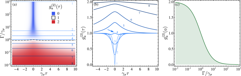
Figure 4: Loss of antibunching of an incoherently driven 2LS due to frequency-filtering. (a) The observed correlations transit from perfect antibunching in the limit in which the frequency of the detected photons is not know ($\Gamma\rightarrow\infty$) to a complete thermalization in the opposite regime ($\Gamma\rightarrow 0$), as predicted by Eq. (32). (b) Cuts of the map in Panel (a) for the $\Gamma/\gamma_{\sigma}$ ratios highlighted by the dashed blue lines shown with small colored numbers 1–8. Note that while the correlations vary from antibunching to bunching, they don’t pass through an exactly uncorrelated emission, as is evidenced by the lump in the correlations marked by the arrow on line 4. (c) Zero-delay correlation as a function of the linewidth of the detector, showing the smooth loss of antibunching due to frequency filtering.

VII.1 incoherent excitation

The master equation in Eq. (9) with the Hamiltonian in Eq. (8) complemented with a detector $\xi$ of bandwidth $\Gamma$ gives access to the frequency-resolved correlations of the incoherently-driven 2LS. When the detector is in resonance to the 2LS, i.e., $\omega_{\xi}=\omega_{\sigma}$, the correlations become

$$g_{\sigma}^{(2)}(\tau)=1-\left(\frac{\Gamma}{\Gamma-\Gamma_{\sigma}}\right)^{2}e^{-\Gamma_{\sigma}\tau}+\frac{\Gamma_{\sigma}(\Gamma_{\sigma}^{2}-3\Gamma\Gamma_{\sigma}-2\Gamma^{2})}{(\Gamma_{\sigma}-\Gamma)^{2}(\Gamma_{\sigma}+3\Gamma)}e^{-\Gamma\tau}+\frac{2\Gamma_{\sigma}\Gamma(5\Gamma-\Gamma_{\sigma})}{(\Gamma_{\sigma}-\Gamma)^{2}(\Gamma_{\sigma}+3\Gamma)}e^{-(\Gamma_{\sigma}+\Gamma)\tau/2}\,,$$ (32)

where $\Gamma_{\sigma}=\gamma_{\sigma}+P_{\sigma}$. This result has been confirmed by independent numerical calculations from frequency-resolved Monte Carlo simulations in Ref. [83]. The expressions for higher-order correlations can also be obtained in a closed form, but they become bulky and typically not considered for antibunching so we do not consider them here. Furthemore, in Ref. [22], we have provided a recurrence relation for all correlations at zero delay. The expression in Eq. (32) is written for positive values of $\tau$, but these correlations are a symmetric function of time, namely $g_{\sigma}^{(2)}(\tau)=g_{\sigma}^{(2)}(-\tau)$, as is shown in Fig. 4. There, one can appreciate the transition form perfect antibunching (in the limit in which the linewidth of the detector is infinite, $\Gamma\rightarrow\infty$, and one does not have information about the frequency of the observed photons), to photon bunching (in the opposite regime, where the linewidth of the detector is much smaller than the linewidth of the emission, $\Gamma/\gamma_{\sigma}\rightarrow 0$) where the extreme frequency filtering yields a thermalization of the signal [85, 86, 50, 22]. Cuts for some values of the detector linewidth are shown in Panel (b), where the various lines (marked with numbers) have a corresponding horizontal dashed line in panel (a). There is a transition of the correlations from antibunching to a thermal state as filtering tightens with an increase of the coherence time. These results have also been previously confirmed through a frequency-resolved Monte Carlo numerical experiment [83]. Note that the isoline $g^{(2)}_{a}(\tau)=1$ is not straight (it is shown as a black dashed-dotted line in the density plot of Fig. 4(a)), and therefore, the passage from antibunching to bunching does not transit through exactly uncorrelated (or coherent light). The shape is similar to that of an antibunched signal contaminated by thermal noise with a smaller coherence time (cf. Eq. (17)) and possibly the effect of the filter could be understood in these terms: as converting some photons from the signal by thermal photons. The particular case of Eq. (32) at zero-delay reduces to

$$g^{(2)}_{\sigma}(0)=\frac{2\Gamma_{\sigma}}{\Gamma_{\sigma}+3\Gamma}\,,$$ (33)

and is shown in Fig. 4(c) (this was also obtained from the cascaded formalism in Ref. [87], Eq. (14b)), where we can appreciate the smooth transition from antibunching to bunching, while also recovering the universal behaviour of thermalization by extreme filtering and of no filtering when detecting at all frequencies, namely

$$\lim_{\Gamma\rightarrow 0}g^{(2)}_{\sigma}(\tau)=2\quad\mathrm{and}\quad\lim_{\Gamma\rightarrow\infty}g^{(2)}_{\sigma}(\tau)=g^{(2)}(\tau)\mathrm{\ of\,\,Eq.~{}(\ref{eq:Thu23Apr2020225637BST})}\,.$$ (34)

A series expansion of $\Gamma$ around zero give the time-dependence for the correlation function for vanishing filters as $g^{(2)}(\tau)\approx 1+\exp(-\Gamma\tau)$, showing how in this case the dynamics of the emitter itself is completely washed out by the filter which is sole responsible for the statistics of the surviving photons. The limit of vanishing frequency-filtering thus deviates qualitatively from the case considered in the previous Section, where the loss of antibunching was due to temporal uncertainty in the measurement. Here, we observe thermalization, with $g_{\sigma}^{(2)}(0)=2$, while in the latter case we observed that the signal became uncorrelated, with $\lim_{\Gamma\rightarrow 0}g^{(2)}_{\Gamma}(\tau)=1$, regardless of the jitter function. This highlights the fundamental difference between the two mechanisms through which the antibunching is lost, with the randomization in the case of temporal uncertainty and the indisitnguishablility bunching stemming from frequency-filtering [86].

The transition is thus richer than one could have expected, although the overal physical behavior matches with expectations. Therefore, Eq. (34) should be more accurately used than the customary single exponential fit $g^{(2)}(\tau)\approx 1-g^{(2)}_{0}\exp(-t/\tau_{0})$, where the value of the parameter $g_{0}$ is introduce from a “deconvolution” of the photon correlations with the temporal profile of the instrument response function (IRF) [52, 53, 54, 55, 56, 57, 58, 59, 60, 61, 62, 63, 64, 65, 66, 67, 68, 69, 70, 71, 72, 73]. The observation of this detailed structure of the loss of antibunching seems to be readily observable experimentally and would consisted a fundamental test of the theory of frequency-resolved photon correlation from the one of the most basic types of quantum emission.

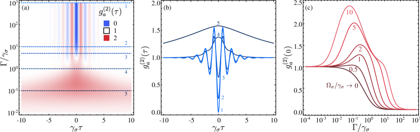
Figure 5: Loss of antibunching of a coherently driven 2LS due to frequency-filtering. (a) The Rabi oscillations induced by the laser are dampened by the frequency filtering, and the perfect antibunching obtained in the limit $\Gamma\rightarrow\infty$ thermalises when $\Gamma=\gamma_{\sigma}$. However, further reducing the linewidth of the detector reveals the uncorrelated nature of the light emitted by the driving laser. (b) Cuts of the density plot in panel (a) illustrating the transition between regimes. (c) The zero-delay correlation of the light emitted by the coherently driven 2LS can be tuned through the linewidth of the detector. The figure corresponds to $\Omega_{\sigma}=2\gamma_{\sigma}$.

VII.2 Coherent excitation

Now turning to Eq. (9) with the Hamiltonian (11) complemented with a detector $\xi$, we obtain the time-resolved frequency-resolved correlations for the coherently-driven 2LS. The general expression can be obtained analytically but it becomes quite cumbersome and will require the definition of a few auxiliary notations. It takes the form of a sum of seven exponentials of $\tau$ correcting the no-correlation value (unity):

$$g^{(2)}_{\sigma}(\tau)=1+\sum_{i=1}^{7}\mathcal{G}_{i}^{(2)}\exp(-\gamma_{i}\tau)$$ (35)

with coherence times

$$\gamma_{1} \equiv(3\gamma_{\sigma}+\gamma_{\mathrm{M}})/4\,,$$ (36a)

$$\gamma_{2} \equiv(3\gamma_{\sigma}-\gamma_{\mathrm{M}})/4\,,$$ (36b)

$$\gamma_{3} \equiv\Gamma/2\,,$$ (36c)

$$\gamma_{4} \equiv\gamma_{{11}}/2\,,$$ (36d)

$$\gamma_{5} \equiv(\gamma_{{23}}+\gamma_{\mathrm{M}})/4\,,$$ (36e)

$$\gamma_{6} \equiv(\gamma_{{23}}-\gamma_{\mathrm{M}})/4\,,$$ (36f)

$$\gamma_{7} \equiv\Gamma\,,$$ (36g)

where we have introduced the notations and

$$\gamma_{{ij}}\equiv i\Gamma+j\gamma_{\sigma}$$ (37)

i.e., $\gamma_{{11}}=\Gamma+\gamma_{\sigma}$ and $\gamma_{{23}}=2\Gamma+3\gamma_{\sigma}$ (a bar means taking the negative number). The corresponding coefficients $\mathcal{G}_{i}$ are bulky and given in Appendix B as Eqs. (61–67), but various limits of interest can be obtained in closed-form of size reasonable enough to be featured as complete expressions, starting with the zero-delay correlation for arbitrary driving intensities:

$$g_{\sigma}^{(2)}(0)=\frac{\gamma_{{11}}(\gamma_{{01}}^{2}+4\Omega^{2})(\gamma_{{11}}\gamma_{{12}}+8\Omega^{2})[\gamma_{{11}}\gamma_{{21}}^{2}\gamma_{{31}}^{2}\gamma_{{12}}\gamma_{{32}}+4\gamma_{{10}}\gamma_{{31}}(17\gamma_{{10}}^{3}+29\gamma_{{10}}^{2}\gamma_{{01}}+18\gamma_{{10}}\gamma_{{01}}^{2}+4\gamma_{{01}}^{3})\Omega^{2}+48\gamma_{{10}}^{2}\gamma_{{21}}\Omega_{0}^{4}]}{\gamma_{{21}}\gamma_{{31}}(\gamma_{{11}}\gamma_{{21}}+4\Omega^{2})(\gamma_{{31}}\gamma_{{32}}+8\Omega^{2})(\gamma_{{11}}^{2}\gamma_{{12}}+4\gamma_{{10}}\Omega^{2})^{2}}\,,$$ (38)

with $\gamma_{{ij}}$ defined in Eq. (37), e.g., $\gamma_{{31}}=3\Gamma+\gamma_{\sigma}$. This was also obtained from the cascaded formalism in Ref. [87], Eq. (19b), and used to account for finite-driving departures in Ref. [42] where this expressions provided an essentially exact fit to the raw data. The time-correlations in the low-driving, Heitler limit can be substantially simplified:

$$g^{(2)}_{\sigma,\mathrm{Heitler}}(\tau)={e^{-(\Gamma+\gamma_{\sigma})\tau}\left(\Gamma^{2}e^{\Gamma\tau/2}-\Gamma\gamma_{\sigma}e^{\gamma_{\sigma}\tau/2}-(\Gamma^{2}-\gamma_{\sigma}^{2})e^{(\Gamma+\gamma_{\sigma})\tau/2}\right)^{2}\over(\Gamma^{2}-\gamma_{\sigma}^{2})^{2}}\,.$$ (39)

with a simple overall behaviour of a monotonous loss of antibunching due to frequency filtering given by:

$$g^{(2)}_{\sigma,\mathrm{Heitler}}(0)=\left(\frac{\gamma_{\sigma}}{\gamma_{\sigma}+\Gamma}\right)^{2}\,.$$ (40)

The high-driving, Mollow regime, on the other hand, is more complex. In particular, taking the limit $\Omega_{\sigma}\to\infty$ sends the satellite peaks away and filtering will be limited to the central peak in this case, which can only produce bunching, namely

$$g^{(2)}_{\sigma,\mathrm{Mollow}\atop 0\ll\Gamma\ll\Omega_{\sigma}}(\tau)=1+2\gamma_{\sigma}{2\Gamma e^{-(\Gamma+\gamma_{\sigma})\tau/2}-(\Gamma+\gamma_{\sigma})e^{-\Gamma\tau}\over(\Gamma-\gamma_{\sigma})(3\Gamma+\gamma_{\sigma})}\,,$$ (41)

with zero-delay coincidences

$$g^{(2)}_{\sigma,\mathrm{Mollow}\atop 0\ll\Gamma\ll\Omega_{\sigma}}(0)={3(\Gamma+\gamma_{\sigma})\over 3\Gamma+\gamma_{\sigma}}\,.$$ (42)

This corresponds to the central part of Fig. 6. The two other parts have to be treated independently and retain the $\Omega_{\sigma}$ dependence, to yield:

$$g^{(2)}_{\sigma,\mathrm{Mollow}\atop\Gamma\to 0}(\tau)= 1+\left({2\gamma_{\sigma}^{2}\over\Omega_{\sigma}^{2}}+{4\Gamma\gamma_{2\overline{1}}\over\gamma_{\sigma}^{2}}\right)e^{-(\Gamma+\gamma_{\sigma})\tau/2}+{3\gamma_{\sigma}^{8}-8\Gamma\gamma_{\sigma}^{4}\gamma_{11}\Omega_{\sigma}^{2}+16\Gamma^{2}(\Gamma\gamma_{5\overline{1}}+\gamma_{\sigma}^{2})\Omega_{\sigma}^{4}\over 8\Gamma^{2}\gamma_{\sigma}^{2}\Omega_{\sigma}^{4}}e^{-\Gamma\tau}$$ (43a)

$$g^{(2)}_{\sigma,\mathrm{Mollow}\atop\Gamma\gg\Omega_{\sigma}}(\tau)= 1+{8(\Gamma/\Omega_{\sigma})^{2}(10+(\Gamma/\Omega_{\sigma})^{2})\over(4+(\Gamma/\Omega_{\sigma})^{2})(8+(\Gamma/\Omega_{\sigma})^{2})^{2}}e^{-\Gamma\tau}-{4(\Gamma/\Omega_{\sigma})^{2}(16+(\Gamma/\Omega_{\sigma})^{2})\over(4+(\Gamma/\Omega_{\sigma})^{2})(8+(\Gamma/\Omega_{\sigma})^{2})^{2}}e^{-(\gamma_{\sigma}+\Gamma)\tau/2}$$

$$+{4(\Gamma/\Omega_{\sigma})^{2}\big{(}(16+(\Gamma/\Omega_{\sigma})^{2}\cos(2\Omega_{\sigma}\tau)+(\Gamma/\Omega_{\sigma})(10+(\Gamma/\Omega_{\sigma})^{2})\sin(2\Omega_{\sigma}\tau)\big{)}\over(4+(\Gamma/\Omega_{\sigma})^{2})(8+(\Gamma/\Omega_{\sigma})^{2})^{2}}e^{-(3\gamma_{\sigma}+2\Gamma)\tau/4}$$ (43b)

$$-{(\Gamma/\Omega_{\sigma})^{2}(16+(\Gamma/\Omega_{\sigma})^{2})\cos(2\Omega_{\sigma}\tau)\over(8+(\Gamma/\Omega_{\sigma})^{2})^{2}}e^{-3\gamma_{\sigma}\tau/4}\,,$$

with corresponding zero-delay correlations:

$$g^{(2)}_{\sigma,\mathrm{Mollow}\atop\Gamma\to 0}(0) ={{\gamma_{41}\gamma_{\sigma}^{9}+12\Gamma\gamma_{21}\gamma_{\sigma}^{6}\Omega_{\sigma}^{2}}{-16\Gamma^{2}\gamma_{\sigma}^{3}\gamma_{14,\overline{5}}\Omega_{\sigma}^{4}-192\Gamma^{3}\gamma_{2\overline{1}}\Omega_{\sigma}^{6}}\over\gamma_{\sigma}(\gamma_{\sigma}^{3}+4\Gamma\Omega_{\sigma}^{2})^{3}}\,,$$ (44a)

$$g^{(2)}_{\sigma,\mathrm{Mollow}\atop\Gamma\gg\Omega_{\sigma}}(0) ={8(2+(\Gamma/\Omega_{\sigma})^{2})(16+(\Gamma/\Omega_{\sigma})^{2})\over(4+(\Gamma/\Omega_{\sigma})^{2})(8+(\Gamma/\Omega_{\sigma})^{2})^{2}}\,,$$ (44b)

which correspond to the left and right parts of Fig. 6, respectively. The simplest formula we can find that unites all these behaviours is the one that is valid for all $\Omega_{\sigma}$ anyway, namely, Eq. (38) to describe the three limits of Eqs. (44a), (42) and (44b) that together reconstruct the curve in Fig. 6(a), and, for the $\tau$ dependence, Eq. (35) along with (36) and (61–67) for the corresponding limits of Eqs. (43a), (41) and (43b). Some of the above results are quite heavy but that only illustrates how rich and complex is the seemingly simple and basic problem of filtering a two-level system and the sort of complexity needed to embody all these various regimes and behaviours in a single analytical expression. One can also check that these results recover those of the unfiltered case in the limit $\Gamma\to\infty$, namely, both Eqs. (35) and (43b) recover Eq. (12), while Eq. (44b) simply recovers the perfect antibunching $g_{\sigma,\Omega\gg\gamma_{\sigma},\Gamma\to\infty}^{(2)}(0)=0$, provided, again, that the limit be taken in the correct order (the filtering should be larger than the Mollow splitting). The situation is, again, simpler in the Heitler regime where also Eqs (39) recovers Eq. (13) and Eq. (40) going to 0, much faster than the Mollow antibunching, as shown in Fig. 6.

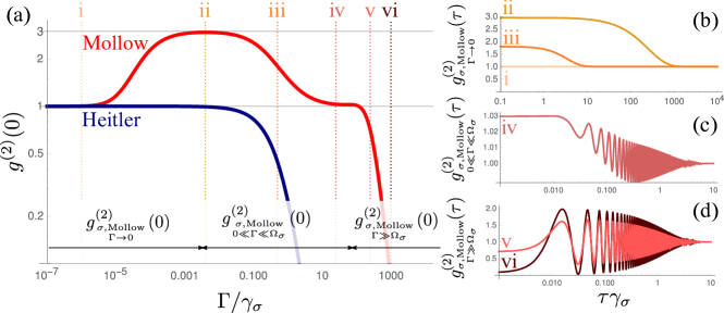
Figure 6: Loss of antibunching for the coherently-driven 2LS both at (a) zero-delay and (b–d) as a function of time $\tau$ in the various limits of the Mollow triplet ($\Omega_{\sigma}\gg\gamma_{\sigma}$ depending on the filter widths: (b) when $\Gamma$ is small, exhibiting bunching, (c) at intermediate $\Gamma$, with onset of correlations and (d) when $\Gamma$ is large and beyond the triplet splitting, exhibiting antibunching. Note that the case iii which belongs to the intermediate regime displays a correlation function akin to those of the low-$\Gamma$ case and is best represented with them. These results can be obtained either from Eqs. (38)–(44) in the corresponding limits or from Eq. (35) that covers all the cases simultaneously (but through a very bulky expression).

We show some temporal correlations for the coherently-driven SPS in Figure 5(a), as a function of time and the linewidth of the detector, for a 2LS with a driving $\Omega_{\sigma}=2\gamma_{\sigma}$, thus well within the Mollow regime of excitation (the loss of antibunching in the Heitler regime has been recently studied in detail both theoretically, along the lines of the current text, and experimentally [73, 42]). On the upper part, where the detector is colorblind, the correlations are given by Eq. (12) and the Rabi oscillations induced by the laser have the maximum visibility [88].

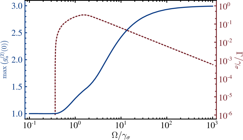
Figure 7: (solid, blue) Maximum value that the zero-delay correlation $g^{(2)}_{\sigma}(0)$ of the coherently-driven 2LS can take for a given driving intensity $\Omega$. At every intensity of the driving, the filter’s linewidth $\Gamma$ has been taken to maximize $g^{(2)}_{\sigma}(0)$ and is shown in dashed, red with values on the right-axis. This shows that a coherently-driven 2LS can always fail to display antibunching depending on the filtering. At $\Omega/\gamma_{\sigma}\lessapprox 0.4$, the filter’s width gets too small to still be featured on the plot but theoretically exists and still remain larger than the $\delta$ function (that has no width) as to produce uncorrelated photons. It would produce bunching otherwise. The qualitative change at about $\Omega/\gamma_{\sigma}\sim 2$ occurs when the three peaks of the Mollow triplet start to be distinguished.

As the linewidth of the detector becomes commensurable with the linewidth of the 2LS, and therefore starts filtering mostly the central peak of the Mollow triplet, the oscillations are softened and vanish completely when the detector filters within a region narrower than the linewidth of the 2LS. Panel (b) shows a series of cuts for several values of $\Gamma/\gamma_{\sigma}$, marked in (a) by dashed lines. The transition from perfect detection in time to perfect detection in frequency can pass through an intermediate regime in which the correlations are bunched. This is clear when focusing on the zero-delay correlations (38), as shown in Fig. 5(c) as a function of the linewidth of the detector for several intensities of the driving. The low-driving case has been observed experimentally by two independent groups [73, 42]. One can observe striking differences with respect to the case of incoherent driving (4(c)): first, the limit of vanishing filtering width leads to randomization rather than to thermalization, thereby behaving like a time-jitter rather than thermal filtering. Such a behaviour is a manifestation of the type of driving and the approximation made to describe the laser as a $\delta$-function, which has exactly zero linewidth. Because of this approximation, one can never filter the photons from within the emission line of the laser, and therefore the thermalization does not appear. However, turning to more sophisticated models of the laser, e.g., the one atom laser [89], then on reaches a thermalization in the limit $\Gamma\rightarrow 0$. The widely used approximation of the laser as a $\delta$-function has nevertheless been shown to be good enough to account for experimental observations several times and under different conditions: mapping the two- and three-photon correlation landscape of the 2LS [90, 91] (in agreement with the theoretical predictions [86, 92]) and recently by measuring the effect of the filter [42] in perturbing the balance between the quantum emission and the laser itself in a self-homodyning picture [93]. In this case, when the linewidth of the filtering is not vanishing, but still remains below the natural linewidth of the 2LS, the correlations become bunched as the intensity of the driving increases. This brings us to the second main departure from the incoherent case, namely, the non-monotonous evolution of $g_{\sigma}^{(2)}(0)$ even if it would thermalize at vanishing $\Gamma$. One can find a region of superbunching with more bunched photons emitted by the 2LS than thermal light itself. The maximum bunching is $g_{\sigma}^{(2)}(0)=3$, as shown in Fig. 7 and is obtained in the limit of high driving and vanishing filtering. This is realized after the observed qualitative change at $\Omega_{\sigma}/\gamma_{\sigma}\geq 1/\sqrt{8}$, when the intensity of the driving is such that the emission spectrum of the 2LS is given by the sum of three Lorentzians [87]. Satisfying the latter condition implies entering into the Mollow triplet regime, and filtering below the natural linewidth of the 2LS means that one is filtering the photons coming from the central peak. The correlations from the photons coming from this region have been predicted to display bunching [94, 79, 86], which has since been observed experimentally [90]. The bunching also observed before that point can be explained by the self-homodyning picture [47], which we do not discuss further as this relate to bunching rather than antibunching that comes with specificities of its own, but this serves to illustrate how the regime of driving result in very different dynamics for the antibunching of the emitter. In particular, the loss of antinbunching is so serious for the coherently-driven 2LS that it complete for all driving intensities, if the filtering is too stringent.

Conclusions and perspectives

We have described a variety of mechanisms—in our understanding the most common and important ones—that lead to a reduction of antibunching with a particular focus on that produced by a two-level system under various regimes of excitations. Much of our results either apply directly to other cases, including both other systems and other types of photon statistics, or could be adapted to systems of interest following the above techniques. For instance, it would be instructive to adapt this analysis to the current record-holder of antibunched emission [6, 7] and track whether the origin of the remaining imperfection lies in the factors analyzed here or in the source itself (i.e., residual re-excitation). We surmise that a perfect antibunched source should not have a Lorentzian profile but feature a standard deviation so as to avoid spurious coincidences from the finite-bandwidth of the detector. This, in itself, however constitutes a different problem.

Even the 2LS system that we have studied above could be analyzed further, e.g., to higher photon-orders, out of resonance with the filter, including other processes such as pure dephasing or phonon-induced dephasing, etc. One could also extend the discussion to other mechanisms that spoil antibunching (some, such as the gravity peak of a streak camera whereby one photon spreads over several pixels of the detectors, are covered in Ref. [39]) or combine those that we have discussed above, from either loss by external noise (Section V), by time uncertainty (or time jitter) (Sec. VI) and/or by frequency filtering (Sec. VII). There are indeed more mechanisms than one would actually want to account for, which lead to a loss of antibunching, and most of them do not constitute in a simple exponential damping of the perfect antibunching of the source. While one particular mechanism (frequency filtering) has been recently investigated in-depth for one of the regimes considered above (Heitler regime) [73, 42], there remains much to confirm experimentally. In particular, the transition frmo antibunching to bunching for the incoherently-driven two-level system, tending to thermalization ruled by the filter alone and passing by an imperfectly uncorrelated state which exhibits a small supression of photon pairs within the emitter’s coherence time when exact coincidences are those of a coherent state ($g^{(2)}(0)=1$), remain to be experimentally demonstrated, a considerable omission for what is arguably the most widely studied quantum optical emitter. The level of agreement with the theory would allow to assess how valid is the two-level picture for the emitter in question, how well-understood is the mechanism leading to its loss of antibunching as well as, at a more fundamental level, how accurate is the theory of frequency-resolved photon correlations, which constitutes in itself a basic aspect of the theory of photodetection.

Appendix: Analytical expresssions

The appendix gives the closed-form analytical expressions which are needed, discussed and/or plotted in the text.

Appendix A Time Jitter

A.1 Heaviside function

The case of the Heaviside function Eq. (26) yields for Eq. (25)

$$g^{(2)}_{\Gamma}(\tau)=\Gamma\int_{\tau}^{\tau+\frac{1}{\Gamma}}\!\!dx\,g^{(2)}(x)[1-\Gamma(x-\tau)]+\theta\left(\tau-\frac{1}{\Gamma}\right)\Gamma\int_{\tau-\frac{1}{\Gamma}}^{\tau}\!\!dx\,g^{(2)}(x)[1+\Gamma(x-\tau)]\\ {}+\theta\left(\frac{1}{\Gamma}-\tau\right)\Gamma\left\{\int_{0}^{\frac{1}{\Gamma}-\tau}\!\!dx\,g^{(2)}(x)\left[1-\Gamma(x+\tau)\right]+{}\right.+\left.\int_{0}^{\tau}\!\!dx\,g^{(2)}(x)\left[1+\Gamma(x-\tau)\right]\right\}\,,$$ (45)

providing the photon correlations from an incoherently driven 2LS with time jitter:

$$g^{(2)}_{\Gamma,P_{\sigma}}(\tau)=1 -{\Gamma^{2}\over\Gamma_{\sigma}^{2}}e^{-\Gamma_{\sigma}(\tau+1/\Gamma)}(1-e^{\Gamma_{\sigma}/\Gamma})^{2}\theta\left(\tau-{1\over\Gamma}\right)$$ (46)

$$-{2\Gamma^{2}\over\Gamma_{\sigma}^{2}}\left\{e^{-\Gamma_{\sigma}/\Gamma}\cosh(\Gamma_{\sigma}\tau)-e^{-\Gamma_{\sigma}\tau}+\Gamma_{\sigma}({1\over\Gamma}-\tau)\right\}\theta\left({1\over\Gamma}-\tau\right)\,,$$ (47)

with the $\tau\geq 1/\Gamma$ behaviour on the first line and $\tau\leq 1/\Gamma$ on the second line, while the corresponding expression for the coherently driven 2LS is

$$g^{(2)}_{\Gamma,\Omega}(\tau)=1-\frac{32\Gamma^{2}e^{-3\gamma_{\sigma}\tau/4}}{R_{\sigma}(R_{\sigma}^{2}+9\gamma_{\sigma}^{2})^{2}}\left[9\gamma_{\sigma}(R_{\sigma}^{2}-3\gamma_{\sigma}^{2})\sin\left(\frac{R_{\sigma}\tau}{4}\right)+R_{\sigma}(R_{\sigma}^{2}-27\gamma_{\sigma}^{2})\cos\left(\frac{R_{\sigma}\tau}{4}\right)\right]+{}\\ {}+\frac{16\Gamma e^{-3\gamma_{\sigma}\tau/4}e^{-3\gamma_{\sigma}/(4\Gamma)}}{R_{\sigma}(R_{\sigma}^{2}+9\gamma_{\sigma}^{2})^{2}}\left\{9\gamma_{\sigma}(R_{\sigma}^{2}-3\gamma_{\sigma}^{2})\sin\left[\frac{R_{\sigma}(1+\Gamma\tau)}{4\Gamma}\right]+R_{\sigma}(R_{\sigma}^{2}-27\gamma_{\sigma}^{2})\cos\left[\frac{R_{\sigma}(1+\Gamma\tau)}{4\Gamma}\right]\right\}+{}\\ {}+\frac{16\Gamma^{2}(R_{\sigma}^{2}-27\gamma_{\sigma}^{2})}{(R_{\sigma}^{2}+9\gamma_{\sigma}^{2})^{2}}\cos\left[\frac{R_{\sigma}(1-\Gamma\tau)}{4\Gamma}\right]e^{-\frac{3\gamma_{\sigma}|1-\Gamma\tau|}{4\Gamma}}-\frac{48\Gamma\gamma_{\sigma}(1-\Gamma\tau)}{R_{\sigma}^{2}+9\gamma_{\sigma}^{2}}\theta\left(\frac{1}{\Gamma}-\tau\right)+{}\\ {}+\frac{144\Gamma^{2}\gamma_{\sigma}(R_{\sigma}^{2}-3\gamma_{\sigma}^{2})}{R_{\sigma}(R_{\sigma}^{2}+9\gamma_{\sigma}^{2})^{2}}\sin\left[\frac{R_{\sigma}(1-\Gamma\tau)}{4\Gamma}\right]\left[e^{-\frac{3\gamma_{\sigma}(1-\Gamma\tau)}{4\Gamma}}\theta\left(\frac{1}{\Gamma}-\tau\right)-e^{\frac{3\gamma_{\sigma}(1-\Gamma\tau)}{4\Gamma}}\theta\left(\tau-\frac{1}{\Gamma}\right)\right]\,.$$ (48)

A.2 Exponential function

In this case, the correlations with time jitter is given by

$$g^{(2)}_{\Gamma}(\tau)=\Gamma\cosh(\Gamma\tau)\int_{0}^{\infty}g^{(2)}(x)e^{-\Gamma x}\,dx-\Gamma\int_{0}^{\tau}\,g^{(2)}(x)\sinh\left[\Gamma(\tau-x)\right]\,dx\,.$$ (49)

In the case of the incoherently driven 2LS, the correlations with time jitter become

$$g^{(2)}_{\Gamma,P_{\sigma}}(\tau)=1-{1\over 1-(\Gamma_{\sigma}/\Gamma)^{2}}\left(e^{-\Gamma_{\sigma}\tau}-(\Gamma_{\sigma}/\Gamma)e^{-\Gamma\tau}\right)\,,$$ (50)

with limit $g^{(2)}_{\Gamma,P_{\sigma}}(\tau)=1-e^{-\Gamma_{\sigma}\tau}(1+\Gamma_{\sigma}\tau)/2$ when $\Gamma=\Gamma_{\sigma}$, whereas the correlations of the coherently driven 2LS become

$$g^{(2)}_{\Gamma,\Omega}(\tau)=1-\frac{j_{1,\Omega}}{N_{+}N_{-}}e^{-\Gamma\tau}-\frac{j_{2,\Omega}}{R_{\sigma}N_{+}N_{-}}e^{-3\gamma_{\sigma}\tau/2}\,,$$ (51)

where $N_{\pm}=R_{\sigma}^{2}+(4\Gamma\pm 3\gamma_{\sigma})^{2}$ and we have defined the functions

$$j_{1,\Omega}=24\Gamma\gamma_{\sigma}(R_{\sigma}^{2}+9\gamma_{\sigma}^{2})\,,$$ (52a)

$$j_{2,\Omega}=16R_{\sigma}\Gamma^{2}(R_{\sigma}^{2}+16\Gamma^{2}-27\gamma_{\sigma}^{2})\cos(R_{\sigma}\tau/4)+48\Gamma^{2}\gamma_{\sigma}(3R_{\sigma}^{2}+16\Gamma^{2}-9\gamma_{\sigma}^{2})\sin(R_{\sigma}\tau/4)\,.$$ (52b)

A.3 Double-exponential

With this function, the expression for the time jitter correlations are given by

$$g^{(2)}_{\Gamma}(\tau)=\Gamma\int_{0}^{\infty}dx\,g^{(2)}(x)e^{-2\Gamma x}\left[(1+2x\Gamma)\cosh(2\Gamma\tau)\right.-{}\\ \left.2\Gamma\tau\sinh(2\Gamma\tau)\right]-\Gamma\int_{0}^{\tau}dx\,g^{(2)}(x)\left\{\sinh[2\Gamma(\tau-x)]-{}\right.\\ \left.{}-2\Gamma(\tau-x)\cosh[2\Gamma(\tau-x)]\right\}\,.$$ (53)

In this case, the correlations of the incoherently driven 2LS, with bare correlations given in Eq. (10), become

$$g^{(2)}_{\Gamma,P_{\sigma}}(\tau)=1-\frac{16}{\Delta^{2}}e^{-\Gamma_{\sigma}\tau}+\frac{(\Gamma_{\sigma}/\Gamma)\big{(}8+\Delta(1+2\Gamma\tau)\big{)}}{\Delta^{2}}e^{-2\Gamma\tau}\,,$$ (54)

where we have used the notation $\Delta\equiv 4-(\Gamma_{\sigma}/\Gamma)^{2}$. The counterpart for the coherent excitation is given by

$$g_{\Gamma,\Omega}^{(2)}(\tau)=1-\frac{g_{1,\Omega}}{\mathcal{N}_{\Omega}}e^{-3\gamma_{\sigma}\tau/4}-\frac{g_{2,\Omega}}{\mathcal{N}_{\Omega}}e^{-2\Gamma\tau}\,,$$ (55)

where we have introduced the functions $g_{1,\Omega}$, $g_{2,\Omega}$ and $\mathcal{N}_{\Omega}$ as follows

$$g_{1,\Omega}=4096\Gamma^{4}\left\{R_{\sigma}\left[(R_{\sigma}^{2}+64\Gamma^{2})^{2}-18(5R_{\sigma}^{2}+192\Gamma^{2})\gamma_{\sigma}^{2}+405\gamma_{\sigma}^{4}\right]\cos(R_{\sigma}\tau/4)+{}\right.\\ \left.{}+3\gamma_{\sigma}\left[5R_{\sigma}^{4}+6R_{\sigma}^{2}(64\Gamma^{2}-15\gamma_{\sigma}^{2})+(64\Gamma^{2}-9\gamma_{\sigma}^{2})^{2}\right]\sin(R_{\sigma}\tau/4)\right\}\,,$$ (56a)

$$g_{2,\Omega}=24R_{\sigma}\Gamma\gamma_{\sigma}(R_{\sigma}^{2}+9\gamma_{\sigma}^{2})+\left\{R_{\sigma}^{4}+384R_{\sigma}^{2}\Gamma^{2}+20480\Gamma^{4}-3456\Gamma^{2}\gamma_{\sigma}^{2}+81\gamma_{\sigma}^{4}+{}\right.\\ \left.{}+2\Gamma[R_{\sigma}^{2}+(8\Gamma-3\gamma_{\sigma})^{2}][R_{\sigma}^{2}+(8\Gamma+3\gamma_{\sigma})^{2}]\tau\right\}\,,$$ (56b)

$$\mathcal{N}_{\Omega}=R_{\sigma}\left[R_{\sigma}^{4}+2R_{\sigma}^{2}(64\Gamma^{2}+9\gamma_{\sigma}^{2})+(64\Gamma^{2}-9\gamma_{\sigma}^{2})^{2}\right]\,.$$ (56c)

A.4 Gaussian

$$g_{\Gamma}^{(2)}(\tau)=\frac{\Gamma}{2\sqrt{\pi}}\int_{0}^{\infty}g^{(2)}(x)\left\{e^{-[(\tau+x)\Gamma/2]^{2}}+e^{-[(\tau-x)\Gamma/2]^{2}}\right\}\,dx\,.$$ (57)

The correlation with time uncertainty for the incoherently driven 2LS becomes

$$g_{\Gamma,P_{\sigma}}^{(2)}(\tau)=1-\frac{e^{(\Gamma_{\sigma}/\Gamma)^{2}}}{2}\left\{e^{-\Gamma_{\sigma}\tau}\mathrm{Erfc}(\tau_{-})+e^{\Gamma_{\sigma}\tau}\mathrm{Erfc}(\tau_{+})\right\}\,,$$ (58)

where $\mathrm{Erfc(\tau)}$ is the complementary error function and we have defined

$$\tau_{\pm}=\frac{\Gamma_{\sigma}}{\Gamma}\pm\frac{\Gamma\tau}{2}\,.$$

The counterpart for coherent excitation has a more complicated structure

$$g_{\Gamma,\Omega}^{(2)}(\tau)=1-\frac{\Delta_{-}}{iR_{\sigma}}e^{(\Delta_{+}/\Gamma)^{2}}h_{1,\Omega}-\frac{\Delta_{+}}{iR_{\sigma}}e^{(\Delta_{-}/\Gamma)^{2}}h_{2,\Omega}\,,$$ (59)

where we have introduced the functions $h_{1,\Omega}$, $h_{2,\Omega}$ and the parameters $\Delta_{\pm}$, defined as

$$h_{1,\Omega}=2\cosh(\Delta_{+}\tau)+\mathrm{Erf}(\lambda_{1,+})e^{\Delta_{+}\tau}+\mathrm{Erf}(\lambda_{1,-})e^{-\Delta_{+}\tau}\,,$$ (60a)

$$h_{2,\Omega}=2\cosh(\Delta_{-}\tau)-\mathrm{Erf}(\lambda_{2,+})e^{\Delta_{-}\tau}-\mathrm{Erf}(\lambda_{2,-})e^{-\Delta_{-}\tau}\,,$$ (60b)

where we have used $\Delta_{\pm}=(iR_{\sigma}\pm 3\gamma_{\sigma})/4$, $\lambda_{1,\pm}=\Delta_{+}/\Gamma\pm\Gamma\tau/2$, $\lambda_{2,\pm}=\Delta_{-}/\Gamma\pm\Gamma\tau/2$ and $R_{\sigma}$ is as defined in Eq. (12).

Appendix B Frequency Filtering

The seven coefficients $\mathcal{G}_{i}$ which, together with the coherence times (36), yield the general two-photon auto-correlation function $g^{(2)}_{\sigma}(\tau)$ for the coherently driven 2LS according to Eq. (35) are given below. They also consist of intricate combinations of the various rates involved, this time also involving subtractions, so that we upgrade Eq. (37)

$$\mathcal{G}_{1}\equiv{\begin{multlined}512\Gamma^{2}\gamma_{11}\Omega_{\sigma}^{2}(\gamma_{11}\gamma_{12}+16\Omega_{\sigma}^{2})(\Gamma\gamma_{1\overline{2}}\gamma_{1\overline{1}}(\gamma_{\mathrm{M}}+\gamma_{\sigma})+8[14\Gamma^{2}+2\gamma_{\sigma}(\gamma_{\mathrm{M}}+\gamma_{\sigma})-\Gamma(7\gamma_{\mathrm{M}}+17\gamma_{\sigma})]\Omega_{\sigma}^{2}-512\Omega_{\sigma}^{4})\\ \kern 5.69046pt\times(\gamma_{11}\gamma_{12}\gamma_{21}(\Gamma(\gamma_{\mathrm{M}}-3\gamma_{\sigma})+2\gamma_{\sigma}(\gamma_{\mathrm{M}}-\gamma_{\sigma}))+8[8\Gamma^{3}+32\Gamma\gamma_{\sigma}^{2}-2\gamma_{\sigma}^{2}(\gamma_{\mathrm{M}}-7\gamma_{\sigma})+\Gamma^{2}(\gamma_{\mathrm{M}}+25\gamma_{\sigma})]\Omega_{\sigma}^{2}+256\Gamma\Omega_{\sigma}^{4})\end{multlined}512\Gamma^{2}\gamma_{11}\Omega_{\sigma}^{2}(\gamma_{11}\gamma_{12}+16\Omega_{\sigma}^{2})(\Gamma\gamma_{1\overline{2}}\gamma_{1\overline{1}}(\gamma_{\mathrm{M}}+\gamma_{\sigma})+8[14\Gamma^{2}+2\gamma_{\sigma}(\gamma_{\mathrm{M}}+\gamma_{\sigma})-\Gamma(7\gamma_{\mathrm{M}}+17\gamma_{\sigma})]\Omega_{\sigma}^{2}-512\Omega_{\sigma}^{4})\\ \kern 5.69046pt\times(\gamma_{11}\gamma_{12}\gamma_{21}(\Gamma(\gamma_{\mathrm{M}}-3\gamma_{\sigma})+2\gamma_{\sigma}(\gamma_{\mathrm{M}}-\gamma_{\sigma}))+8[8\Gamma^{3}+32\Gamma\gamma_{\sigma}^{2}-2\gamma_{\sigma}^{2}(\gamma_{\mathrm{M}}-7\gamma_{\sigma})+\Gamma^{2}(\gamma_{\mathrm{M}}+25\gamma_{\sigma})]\Omega_{\sigma}^{2}+256\Gamma\Omega_{\sigma}^{4})\over\gamma_{\mathrm{M}}(\gamma_{\mathrm{M}}-\Gamma)(\gamma_{\mathrm{M}}-\gamma_{\sigma})(\gamma_{\mathrm{M}}+\gamma_{\sigma})^{2}(\gamma_{\mathrm{M}}+\gamma_{\sigma}-2\Gamma)(\gamma_{\mathrm{M}}+3\gamma_{\sigma}-4\Gamma)(\gamma_{\mathrm{M}}+3\gamma_{\sigma}-2\Gamma)(\gamma_{11}\gamma_{21}+8\Omega_{\sigma}^{2})(\gamma_{11}^{2}\gamma_{12}+8\Gamma\Omega_{\sigma}^{2})^{2}}$$ (61)

$$\mathcal{G}_{2}\equiv\mathcal{G}_{1}\ \hbox{with }\gamma_{\mathrm{M}}\leftrightarrow-\gamma_{\mathrm{M}}$$ (62)

$$\mathcal{G}_{3}\equiv 2{256\Gamma\gamma_{11}\gamma_{\sigma}\Omega_{\sigma}^{2}(\gamma_{11}\gamma_{12}+16\Omega_{\sigma}^{2})(\gamma_{11}^{2}\gamma_{12}\gamma_{1\overline{2}}\gamma_{21}^{2}+8\gamma_{11}(9\Gamma^{3}+20\Gamma\gamma_{\sigma}\gamma_{11}+8\gamma_{\sigma}^{3})\Omega_{\sigma}^{2}+128\Gamma^{2}\Omega_{\sigma}^{4})\over\gamma_{11}^{2}\gamma_{21}(\gamma_{\mathrm{M}}^{2}-\gamma_{\sigma}^{2})(\gamma_{\mathrm{M}}^{2}-\gamma_{2\overline{3}}^{2})(\gamma_{11}\gamma_{21}+8\Omega_{\sigma}^{2})(\gamma_{12}+8\Gamma\Omega_{\sigma}^{2})^{2}}$$ (63)

$$\mathcal{G}_{4}\equiv 2{2\Gamma^{3}(\gamma_{\sigma}^{2}+8\Omega_{\sigma}^{2})(\gamma_{11}\gamma_{12}+16\Omega_{\sigma}^{2})(\gamma_{11}^{2}\gamma_{12}^{2}\gamma_{31}+48\Gamma\gamma_{11}^{2}\Omega_{\sigma}^{2}-256\gamma_{\sigma}\Omega_{\sigma}^{4})\over\gamma_{1\overline{1}}\gamma_{31}(\gamma_{\mathrm{M}}^{2}-\gamma_{2\overline{1}}^{2})(\gamma_{11}\gamma_{21}+8\Omega_{\sigma}^{2})(\gamma_{11}^{2}\gamma_{12}+8\Gamma\Omega_{\sigma}^{2})^{2}}$$ (64)

$$\mathcal{G}_{5}\equiv 2\frac{\begin{multlined}-1024\Gamma^{2}\gamma_{11}\Omega_{\sigma}^{4}\Big{[}\gamma_{11}^{2}\gamma_{12}^{2}\gamma_{21}\gamma_{31}\gamma_{32}\big{(}2\Gamma^{2}(\gamma_{\mathrm{M}}-3\gamma_{\sigma})-\Gamma\gamma_{\sigma}(\gamma_{\mathrm{M}}+3\gamma_{\sigma})-2\gamma_{\sigma}^{2}(\gamma_{\mathrm{M}}-\gamma_{\sigma})\big{)}+{}\\ {}+8\gamma_{11}\gamma_{12}\Omega_{\sigma}^{2}\Big{\{}-108\Gamma^{6}+\Gamma^{5}(215\gamma_{\mathrm{M}}-1203\gamma_{\sigma})+3\Gamma^{4}\gamma_{\sigma}(239\gamma_{\mathrm{M}}-1081\gamma_{\sigma})+\Gamma^{3}\gamma_{\sigma}^{2}(1051\gamma_{\mathrm{M}}-3947\gamma_{\sigma})+{}\\ \hskip 73.12378pt{}+\Gamma^{2}\gamma_{\sigma}^{3}(803\gamma_{\mathrm{M}}-2465\gamma_{\sigma})+10\Gamma\gamma_{\sigma}^{4}(31\gamma_{\mathrm{M}}-77\gamma_{\sigma})+48\gamma_{\sigma}^{5}(\gamma_{\mathrm{M}}+2\gamma_{\sigma})\Big{\}}+{}\\ {}+128\Omega_{\sigma}^{4}\Big{\{}6\Gamma^{6}+\Gamma^{5}(131\gamma_{\mathrm{M}}-227\gamma_{\sigma})+\Gamma^{4}\gamma_{\sigma}(546\gamma_{\mathrm{M}}-776\gamma_{\sigma}^{2})+\Gamma^{3}\gamma_{\sigma}^{2}(889\gamma_{\mathrm{M}}-933\gamma_{\sigma})+{}\\ +\Gamma^{2}\gamma_{\sigma}^{3}(724\gamma_{\mathrm{M}}-488\gamma_{\sigma})+\Gamma\gamma_{\sigma}^{4}(296\gamma_{\mathrm{M}}-96\gamma_{\sigma})+48\gamma_{\mathrm{M}}\gamma_{\sigma}^{5}\Big{\}}+{}\\ {}+2048\Omega_{\sigma}^{6}\Big{\{}74\Gamma^{4}+2\Gamma^{3}(6\gamma_{\mathrm{M}}+109\gamma_{\sigma})+5\Gamma^{2}\gamma_{\sigma}(3\gamma_{\mathrm{M}}+61\gamma_{\sigma})+2\Gamma\gamma_{\sigma}^{2}(-\gamma_{\mathrm{M}}+103\gamma_{\sigma})-4\gamma_{\sigma}^{3}(\gamma_{\mathrm{M}}-13\gamma_{\sigma})\Big{\}}+{}\\ {}+131072\Gamma\gamma_{21}\Omega_{\sigma}^{8}\Big{]}\end{multlined}-1024\Gamma^{2}\gamma_{11}\Omega_{\sigma}^{4}\Big{[}\gamma_{11}^{2}\gamma_{12}^{2}\gamma_{21}\gamma_{31}\gamma_{32}\big{(}2\Gamma^{2}(\gamma_{\mathrm{M}}-3\gamma_{\sigma})-\Gamma\gamma_{\sigma}(\gamma_{\mathrm{M}}+3\gamma_{\sigma})-2\gamma_{\sigma}^{2}(\gamma_{\mathrm{M}}-\gamma_{\sigma})\big{)}+{}\\ {}+8\gamma_{11}\gamma_{12}\Omega_{\sigma}^{2}\Big{\{}-108\Gamma^{6}+\Gamma^{5}(215\gamma_{\mathrm{M}}-1203\gamma_{\sigma})+3\Gamma^{4}\gamma_{\sigma}(239\gamma_{\mathrm{M}}-1081\gamma_{\sigma})+\Gamma^{3}\gamma_{\sigma}^{2}(1051\gamma_{\mathrm{M}}-3947\gamma_{\sigma})+{}\\ \hskip 73.12378pt{}+\Gamma^{2}\gamma_{\sigma}^{3}(803\gamma_{\mathrm{M}}-2465\gamma_{\sigma})+10\Gamma\gamma_{\sigma}^{4}(31\gamma_{\mathrm{M}}-77\gamma_{\sigma})+48\gamma_{\sigma}^{5}(\gamma_{\mathrm{M}}+2\gamma_{\sigma})\Big{\}}+{}\\ {}+128\Omega_{\sigma}^{4}\Big{\{}6\Gamma^{6}+\Gamma^{5}(131\gamma_{\mathrm{M}}-227\gamma_{\sigma})+\Gamma^{4}\gamma_{\sigma}(546\gamma_{\mathrm{M}}-776\gamma_{\sigma}^{2})+\Gamma^{3}\gamma_{\sigma}^{2}(889\gamma_{\mathrm{M}}-933\gamma_{\sigma})+{}\\ +\Gamma^{2}\gamma_{\sigma}^{3}(724\gamma_{\mathrm{M}}-488\gamma_{\sigma})+\Gamma\gamma_{\sigma}^{4}(296\gamma_{\mathrm{M}}-96\gamma_{\sigma})+48\gamma_{\mathrm{M}}\gamma_{\sigma}^{5}\Big{\}}+{}\\ {}+2048\Omega_{\sigma}^{6}\Big{\{}74\Gamma^{4}+2\Gamma^{3}(6\gamma_{\mathrm{M}}+109\gamma_{\sigma})+5\Gamma^{2}\gamma_{\sigma}(3\gamma_{\mathrm{M}}+61\gamma_{\sigma})+2\Gamma\gamma_{\sigma}^{2}(-\gamma_{\mathrm{M}}+103\gamma_{\sigma})-4\gamma_{\sigma}^{3}(\gamma_{\mathrm{M}}-13\gamma_{\sigma})\Big{\}}+{}\\ {}+131072\Gamma\gamma_{21}\Omega_{\sigma}^{8}\Big{]}}{\gamma_{21}\gamma_{\mathrm{M}}(\gamma_{\mathrm{M}}+\Gamma)(\gamma_{\mathrm{M}}-\gamma_{\sigma})(\gamma_{\mathrm{M}}+\gamma_{\sigma})^{2}(\gamma_{\mathrm{M}}-\gamma_{2\overline{3}})(\gamma_{11}\gamma_{21}+8\Omega_{\sigma}^{2})(\gamma_{11}^{2}\gamma_{12}+8\Gamma\Omega_{\sigma}^{2})^{2}(\gamma_{31}\gamma_{32}+16\Omega_{\sigma}^{2})}$$ (65)

$$\mathcal{G}_{6}\equiv\mathcal{G}_{5}\ \text{with }\gamma_{\mathrm{M}}\leftrightarrow-\gamma_{\mathrm{M}}$$ (66)

$$\mathcal{G}_{7}\equiv{\begin{multlined}32\Gamma^{2}\gamma_{11}(\gamma_{\sigma}^{2}+8\Omega_{\sigma}^{2})\Big{[}(\gamma_{11}\gamma_{12}+16\Omega_{\sigma}^{2})(\gamma_{11}\gamma_{12}\gamma_{21}^{2}\gamma_{31}^{2}\gamma_{32}\gamma_{1\overline{1}}\gamma_{1\overline{2}}\gamma_{2\overline{1}})+{}\\ \hskip 28.45274pt{}+8\gamma_{31}\Omega_{\sigma}^{2}\{142\Gamma^{7}+239\Gamma^{6}\gamma_{\sigma}-241\Gamma^{5}\gamma_{\sigma}^{2}-677\Gamma^{4}\gamma_{\sigma}^{3}+77\Gamma^{3}\gamma_{\sigma}^{4}+832\Gamma^{2}\gamma_{\sigma}^{5}+580^{\Gamma}\gamma_{\sigma}^{6}+128\gamma_{\sigma}^{7}\}+{}\\ +64\Omega_{\sigma}^{4}\{219\Gamma^{6}+386\Gamma^{5}\gamma_{\sigma}+565\Gamma^{4}\gamma_{\sigma}^{2}+344\Gamma^{3}\gamma_{\sigma}^{3}-98\Gamma^{2}\gamma_{\sigma}^{4}-208\Gamma\gamma_{\sigma}^{5}-56\gamma_{\sigma}^{6}\}+{}\\ +1024\Omega_{\sigma}^{6}\{15\Gamma^{4}-11\Gamma^{3}\gamma_{\sigma}-4\Gamma^{2}\gamma_{\sigma}^{2}-16\Gamma\gamma_{\sigma}^{3}-8\gamma_{\sigma}^{4}\}-16384\Omega_{\sigma}^{8}\gamma_{\sigma}\gamma_{21}\Big{]}\end{multlined}32\Gamma^{2}\gamma_{11}(\gamma_{\sigma}^{2}+8\Omega_{\sigma}^{2})\Big{[}(\gamma_{11}\gamma_{12}+16\Omega_{\sigma}^{2})(\gamma_{11}\gamma_{12}\gamma_{21}^{2}\gamma_{31}^{2}\gamma_{32}\gamma_{1\overline{1}}\gamma_{1\overline{2}}\gamma_{2\overline{1}})+{}\\ \hskip 28.45274pt{}+8\gamma_{31}\Omega_{\sigma}^{2}\{142\Gamma^{7}+239\Gamma^{6}\gamma_{\sigma}-241\Gamma^{5}\gamma_{\sigma}^{2}-677\Gamma^{4}\gamma_{\sigma}^{3}+77\Gamma^{3}\gamma_{\sigma}^{4}+832\Gamma^{2}\gamma_{\sigma}^{5}+580^{\Gamma}\gamma_{\sigma}^{6}+128\gamma_{\sigma}^{7}\}+{}\\ +64\Omega_{\sigma}^{4}\{219\Gamma^{6}+386\Gamma^{5}\gamma_{\sigma}+565\Gamma^{4}\gamma_{\sigma}^{2}+344\Gamma^{3}\gamma_{\sigma}^{3}-98\Gamma^{2}\gamma_{\sigma}^{4}-208\Gamma\gamma_{\sigma}^{5}-56\gamma_{\sigma}^{6}\}+{}\\ +1024\Omega_{\sigma}^{6}\{15\Gamma^{4}-11\Gamma^{3}\gamma_{\sigma}-4\Gamma^{2}\gamma_{\sigma}^{2}-16\Gamma\gamma_{\sigma}^{3}-8\gamma_{\sigma}^{4}\}-16384\Omega_{\sigma}^{8}\gamma_{\sigma}\gamma_{21}\Big{]}\over\gamma_{21}\gamma_{31}\gamma_{1\overline{1}}(\gamma_{\mathrm{M}}^{2}-\gamma_{3\overline{2}}^{2})(\gamma_{\mathrm{M}}^{2}-\gamma_{4\overline{3}}^{2})(\gamma_{11}\gamma_{21}+8\Omega_{\sigma}^{2})(\gamma_{11}\gamma_{12}+8\Omega_{\sigma}^{2})(\gamma_{31}\gamma_{32}+16\Omega_{\sigma}^{2})}$$ (67)

While these expressions are not particularly enlightening, they provide the most general and exact closed-form formula for the filtered coherently-driven 2LS. One cannot but marvel at how Mathematics bring in unexpected factors, 7, 17, 20, to thwart cancellations of these expression so as to ultimately provide what we interpretate in physical terms, such as an elbow in a curve that correspond to the Mollow triplet splitting into three spectral lines.

References

- Paul [1982] H. Paul, Photon antibunching, Rev. Mod. Phys. 54, 1061 (1982).
- Hanbury Brown and Twiss [1956a] R. Hanbury Brown and R. Q. Twiss, A test of a new type of stellar interferometer on Sirius, Nature 178, 1046 (1956a).
- Kimble et al. [1977] H. J. Kimble, M. Dagenais, and L. Mandel, Photon antibunching in resonance fluorescence, Phys. Rev. Lett. 39, 691 (1977).
- Kuhlmann et al. [2015] A. V. Kuhlmann, J. H. Prechtel, J. Houel, A. Ludwig, D. Reuter, A. D. Wieck, and R. J. Warburton, Transform-limited single photons from a single quantum dot, Nature Comm. 6, 8204 (2015).
- Gallop [1990] J. C. Gallop, SQUIDS, the Josephson Effects and Superconducting Electronics (CRC press, 1990).
- Schweickert et al. [2018] L. Schweickert, K. D. Jöns, K. D. Zeuner, S. F. C. da Silva, H. Huang, T. Lettner, M. Reindl, J. Zichi, R. Trotta, A. Rastelli, and V. Zwiller, On-demand generation of background-free single photons from a solid-state source, Appl. Phys. Lett. 112, 093106 (2018).
- Hanschke et al. [2018] L. Hanschke, K. A. Fischer, S. Appel, D. Lukin, J. Wierzbowski, S. Sun, R. Trivedi, J. Vuc̆ković, J. J. Finley, and K. Müller, Quantum dot single-photon sources with ultra-low multi-photon probability, npj Quantum Information 4, 43 (2018).
- Müller et al. [2014] M. Müller, S. Bounouar, K. D. Jöns, M. Glässl, and P. Michler, On-demand generation of indistinguishable polarization-entangled photon pairs, Nature Photon. 8, 224 (2014).
- Wei et al. [2014] Y.-J. Wei, Y.-M. He, M.-C. Chen, Y.-N. Hu, Y. He, D. Wu, C. Schneider, M. Kamp, S. Höfling, C.-Y. Lu, and J.-W. Pan, Deterministic and robust generation of single photons from a single quantum dot with 99.5% indistinguishability using adiabatic rapid passage, Nano Lett. 14, 6515 (2014).
- Sapienza et al. [2015] L. Sapienza, M. Davanço, A. Badolato, and K. Srinivasa, Nanoscale optical positioning of single quantum dots for bright and pure single-photon emission, Nature Comm. 6, 7833 (2015).
- Miyazawa et al. [2016] T. Miyazawa, K. Takemoto, Y. Nambu, S. Miki, T. Yamashita, H. Terai, M. Fujiwara, M. Sasaki, Y. Sakuma, M. Takatsu, T. Yamamoto, and Y. Arakawa, Single-photon emission at 1.5 m from an InAs/InP quantum dot with highly suppressed multi-photon emission probabilities, Appl. Phys. Lett. 109, 132106 (2016).
- Ding et al. [2016] X. Ding, Y. He, Z.-C. Duan, N. Gregersen, M.-C. Chen, S. Unsleber, S. Maier, C. Schneider, M. Kamp, S. Höfling, C.-Y. Lu, and J.-W. Pan, On-demand single photons with high extraction efficiency and near-unity indistinguishability from a resonantly driven quantum dot in a micropillar, Phys. Rev. Lett. 116, 020401 (2016).
- Somaschi et al. [2016] N. Somaschi, V. Giesz, L. D. Santis, J. C. Loredo, M. P. Almeida, G. Hornecker, S. L. Portalupi, T. Grange, C. Antón, J. Demory, C. Gómez, I. Sagnes, N. D. Lanzillotti-Kimura, A. Lemaître, A. Auffeves, A. G. White, L. Lanco, and P. Senellart, Near-optimal single-photon sources in the solid state, Nature Photon. 10, 340 (2016).
- Unsleber et al. [2016] S. Unsleber, Y.-M. He, S. Gerhardt, S. Maier, C.-Y. Lu, J.-W. Pan, N. Gregersen, M. Kamp, C. Schneider, and S. Höfling, Highly indistinguishable on-demand resonance fluorescence photons from a deterministic quantum dot micropillar device with 74% extraction efficiency, Opt. Express 24, 8539 (2016).
- Wang et al. [2016] H. Wang, Z.-C. Duan, Y.-H. Li, S. Chen, J.-P. Li, Y.-M. He, M.-C. Chen, Y. He, X. Ding, C.-Z. Peng, C. Schneider, M. Kamp, S. Höfling, C.-Y. Lu, and J.-W. Pan, Near-transform-limited single photons from an efficient solid-state quantum emitter, Phys. Rev. Lett. 116, 213601 (2016).
- Higginbottom et al. [2016] D. B. Higginbottom, L. Slodička, G. Araneda, L. Lachman, R. Filip, M. Hennrich, and R. Blatt, Pure single photons from a trapped atom source, New J. Phys. 18, 093038 (2016).
- Huber et al. [2017] D. Huber, M. Reindl, Y. Huo, H. Huang, J. S. Wildmann, O. G. Schmidt, A. Rastelli, and R. Trotta, Highly indistinguishable and strongly entangled photons from symmetric GaAs quantum dots, Nature Comm. 8, 15506 (2017).
- Senellart et al. [2017] P. Senellart, G. Solomon, and A. White, High-performance semiconductor quantum-dot single-photon sources, Nature Nanotech. 12, 1026 (2017).
- Liu et al. [2018a] J. Liu, K. Konthasinghe, M. Davanço, J. Lawall, V. Anant, V. Verma, R. Mirin, S. W. Nam, J. D. Song, B. Ma, Z. S. Chen, H. Q. Ni, Z. C. Niu, and K. Srinivasan, Single self-assembled InAs/GaAs quantum dots in photonic nanostructures: The role of nanofabrication, Phys. Rev. Appl. 9, 064019 (2018a).
- Musiał et al. [2020] A. Musiał, P. Holewa, P. Wyborski, M. Syperek, A. Kors, J. P. Reithmaier, G. S\kek, and M. Benyoucef, High-purity triggered single-photon emission from symmetric single InAs/InP quantum dots around the telecom C-band window, Adv. Quantum Technol. 3, 1900082 (2020).
- Arakawa and Holmes [2020] Y. Arakawa and M. J. Holmes, Progress in quantum-dot single photon sources for quantum information technologies: A broad spectrum overview, Appl. Phys. Rev. 7, 021309 (2020).
- López Carreño et al. [2016] J. C. López Carreño, C. Sánchez Muñoz, E. del Valle, and F. P. Laussy, Excitation with quantum light. II. Exciting a two-level system, Phys. Rev. A 94, 063826 (2016).
- Teich and Saleh [1988] M. C. Teich and B. E. A. Saleh, Photon bunching and antibunching, Progress in Optics 26, 1 (1988).
- Glauber [1963] R. J. Glauber, Coherent and incoherent states of the radiation field, Phys. Rev. 131, 2766 (1963).
- Mandel and Wolf [1995] L. Mandel and E. Wolf, Optical coherence and quantum optics (Cambridge University Press, Cambridge, 1995).
- Scully and Zubairy [2002] M. O. Scully and M. S. Zubairy, Quantum optics (Cambridge University Press, 2002).
- C.Teich et al. [2983] M. C.Teich, B. E. A. Saleh, and D. Stoler, Antibunching in the franck-hertz experiment, Opt. Commun. 46, 244 (2983).
- Zou and Mandel [1990] X. T. Zou and L. Mandel, Photon-antibunching and sub-poissonian photon statistics, Phys. Rev. A 41, 475 (1990).
- Hanbury Brown et al. [1952] R. Hanbury Brown, R. C. Jennison, and M. K. D. Gupta, Apparent angular sizes of discrete radio sources: Observations at Jodrell Bank, Manchester, Nature 170, 1061 (1952).
- Hanbury Brown and Twiss [1954] R. Hanbury Brown and R. Twiss, A new type of interferometer for use in radio astronomy, Phil. Mag. 45, 663 (1954).
- Hanbury Brown and Twiss [1956b] R. Hanbury Brown and R. Q. Twiss, Correlation between photons in two coherent beams of light, Nature 177, 27 (1956b).
- Purcell [1956] E. M. Purcell, The question of correlation between photons in coherent light rays, Nature 178, 1449 (1956).
- Stoler [1974] D. Stoler, Photon antibunching and possible ways to observe it, Phys. Rev. Lett. 33, 1397 (1974).
- Silberhorn [2007] C. Silberhorn, Detecting quantum light, Contemporary Physics 48, 143 (2007).
- Kardynał et al. [2008] B. E. Kardynał, Z. L. Yuan, and A. J. Shields, An avalanche‐photodiode-based photon-number-resolving detector, Nature Photon. 2, 425 (2008).
- Hadfield [2009] R. H. Hadfield, Single-photon detectors for optical quantum information applications, Nature Photon. 3, 696 (2009).
- Yuan et al. [2007] Z. L. Yuan, B. E. Kardynal, A. W. Sharpe, and A. J. Shields, High speed single photon detection in the near infrared, Appl. Phys. Lett. 91, 041114 (2007).
- Wiersig et al. [2009] J. Wiersig, C. Gies, F. Jahnke, M. Aßmann, T. Berstermann, M. Bayer, C. Kistner, S. Reitzenstein, C. Schneider, S. Höfling, A. Forchel, C. Kruse, J. Kalden, and D. Homme, Direct observation of correlations between individual photon emission events of a microcavity laser, Nature 460, 245 (2009).
- Silva [2016] B. Silva, Reaching Quantum Polaritons, Ph.D. thesis, Universidad Autónoma de Madrid (2016).
- Klaas et al. [2018] M. Klaas, E. Schlottmann, H. Flayac, F. Laussy, F. Gericke, M. Schmidt, M. Helversen, J. Beyer, S. Brodbeck, H. Suchomel, S. Höfling, S. Reitzenstein, and C. Schneider, Photon-number-resolved measurement of an exciton-polariton condensate, Phys. Rev. Lett. 121, 047401 (2018).
- Bachor and Ralph [2004] H.-A. Bachor and T. C. Ralph, A guide to experiments in quantum optics (Wiley, 2004).
- Hanschke et al. [2020] L. Hanschke, L. Schweickert, J. C. L. Carreño, E. Schöll, K. D. Zeuner, T. Lettner, E. Z. Casalengua, M. Reindl, S. F. C. da Silva, R. Trotta, J. J. Finley, A. Rastelli, E. del Valle, F. P. Laussy, V. Zwiller, K. Müller, and K. D. Jöns, Origin of antibunching in resonance fluorescence, Phys. Rev. Lett. 125, 10402 (2020).
- Heitler [1944] W. Heitler, The Quantum Theory of Radiation (Oxford University Press, 1944).
- Stucki et al. [2001] D. Stucki, G. Ribordy, A. Stefanov, H. Zbinden, J. G. Rarity, and T. Wall, Photon counting for quantum key distribution with peltier cooled InGaAs/InP APDs, J. Mod. Opt. 48, 1967 (2001).
- Yuan et al. [2009] L. Yuan, Z. Yu-Chi, Z. Peng-Fei, G. Yan-Qiang, L. Gang, W. Jun-Min, and Z. Tian-Cai, Experimental study on coherence time of a light field with single photon counting, Chinese Phys. Lett. 26, 074205 (2009).
- Teich and Saleh [1982] M. C. Teich and B. E. A. Saleh, Effects of random deletion and additive noise on bunched and antibunched photon-counting statistics, Opt. Lett. 7, 365 (1982).
- Zubizarreta Casalengua et al. [2020a] E. Zubizarreta Casalengua, J. C. López Carreño, F. P. Laussy, and E. del Valle, Tuning photon statistics with coherent fields, Phys. Rev. A 101, 063824 (2020a).
- Eberly and Wódkiewicz [1977] J. Eberly and K. Wódkiewicz, The time-dependent physical spectrum of light, J. Opt. Soc. Am. 67, 1252 (1977), tDS1.3.
- del Valle et al. [2012] E. del Valle, A. González-Tudela, F. P. Laussy, C. Tejedor, and M. J. Hartmann, Theory of frequency-filtered and time-resolved -photon correlations, Phys. Rev. Lett. 109, 183601 (2012).
- Silva et al. [2016] B. Silva, C. S. Muñoz, D. Ballarini, A. González-Tudela, M. de Giorgi, G. Gigli, K. West, L. Pfeiffer, E. del Valle, D. Sanvitto, and F. P. Laussy, The colored Hanbury Brown–Twiss effect, Sci. Rep. 6, 37980 (2016).
- Ulrich et al. [2007] S. M. Ulrich, C. Gies, S. Ates, J. Wiersig, S. Reitzenstein, C. Hofmann, A. Löffler, A. Forchel, F. Jahnke, and P. Michler, Photon statistics of semiconductor microcavity lasers, Phys. Rev. Lett. 98, 043906 (2007).
- Michler et al. [2000] P. Michler, A. Kiraz, C. Becher, W. V. Schoenfeld, P. M. Petroff, L. Zhang, E. Hu, and A. Ĭmamoḡlu, A quantum dot single-photon turnstile device, Science 290, 2282 (2000).
- Fleury et al. [2000] L. Fleury, J.-M. Segura, G. Zumofen, B. Hecht, and U. P. Wild, Nonclassical photon statistics in single-molecule fluorescence at room temperature, Phys. Rev. Lett. 84, 1148 (2000).
- Kurtsiefer et al. [2000] C. Kurtsiefer, S. Mayer, P. Zarda, and H. Weinfurter, Stable solid-state source of single photons, Phys. Rev. Lett. 85, 290 (2000).
- Messin et al. [2001] G. Messin, J. P. Karr, A. Baas, G. Khitrova, R. Houdré, R. P. Stanley, U. Oesterle, and E. Giacobino, Parametric polariton amplification in semiconductor microcavities, Phys. Rev. Lett. 87, 127403 (2001).
- Flagg et al. [2009] E. B. Flagg, A. Muller, J. W. Robertson, S. Founta, D. G. Deppe, M. Xiao, W. Ma, G. J. Salamo, and C. K. Shih, Resonantly driven coherent oscillations in a solid-state quantum emitter, Nature Phys. 5, 203 (2009).
- Nothaft et al. [2012] M. Nothaft, S. Höhla, F. Jelezko, N. Frühauf, J. Pflaum, and J. Wrachtrup, Electrically driven photon antibunching from a single molecule at room temperature, Nature Comm. 3, 628 (2012).
- Konthasinghe et al. [2012] K. Konthasinghe, J. Walker, M. Peiris, C. K. Shih, Y. Yu, M. F. Li, J. F. He, L. J. Wang, H. Q. Ni, Z. C. Niu, and A. Muller, Coherent versus incoherent light scattering from a quantum dot, Phys. Rev. B (2012).
- Matthiesen et al. [2012] C. Matthiesen, A. N. Vamivakas, and M. Atatüre, Subnatural linewidth single photons from a quantum dot, Phys. Rev. Lett. 108, 093602 (2012).
- He et al. [2013] Y.-M. He, Y. He, Y.-J. Wei, D. Wu, M. Atatüre, C. Schneider, S. Höfling, M. Kamp, C.-Y. Lu, and J.-W. Pan, On-demand semiconductor single-photon source with near-unity indistinguishability, Nature Nanotech. 8, 213 (2013).
- Reithmaier et al. [2015] G. Reithmaier, M. Kaniber, F. Flassig, S. Lichtmannecker, K. Müller, A. Andrejew, J. Vučković, R. Gross, and J. J. Finley, On-chip generation, routing, and detection of resonance fluorescence, Nano Lett. 15, 5208 (2015).
- He et al. [2015] Y. He, Y.-M. He, J. Liu, Y.-J. Wei, H. Ramírez, M. Atatüre, C. Schneider, M. Kamp, S. Höfling, C.-Y. Lu, , and J.-W. Pan, Dynamically controlled resonance fluorescence spectra from a doubly dressed single ingaas quantum dot, Phys. Rev. Lett. 114, 097402 (2015).
- Kumar et al. [2016] S. Kumar, M. Brotóns-Gisbert, R. Al-Khuzheyri, A. Branny, G. Ballesteros-Garcia, J. F. Sánchez-Royo, and B. Gerardot, Resonant laser spectroscopy of localized excitons in monolayer WSe2, Optica 3, 882 (2016).
- Malein et al. [2016] R. N. E. Malein, T. S. Santana, J. M. Zajac, A. C. Dada, E. M. Gauger, P. M. Petroff, J. Y. Lim, J. D. Song, and B. Gerardot, Screening nuclear field fluctuations in quantum dots for indistinguishable photon generation, Phys. Rev. Lett. 116, 257401 (2016).
- Gao et al. [2017] S. Gao, M. Cui, R. Li, L. Liang, Y. Liu, and L. Xie, Quantitative deconvolution of autocorrelations and cross correlations from two-dimensional lifetime decay maps in fluorescence lifetime correlation spectroscopy, Sci. Bull. 62, 9 (2017).
- Snijders et al. [2018] H. Snijders, J. Frey, J. Norman, H. Flayac, V. Savona, A. Gossard, J. Bowers, M. van Exter, D. Bouwmeester, and W. Löffler, Observation of the unconventional photon blockade, Phys. Rev. Lett. 121, 043601 (2018).
- Zhao et al. [2018] S. Zhao, J. Lavie, L. Rondin, L. Orcin-Chaix, C. Diederichs, P. Roussignol, Y. Chassagneux, C. Voisin, K. Müllen, A. Narita, S. Campidelli, and J.-S. Lauret, Single photon emission from graphene quantum dots at room temperature, Nature Comm. 9, 3470 (2018).
- Fink et al. [2018] T. Fink, A. Schade, S. Höfling, C. Schneider, and A. Ĭmamoḡlu, Signatures of a dissipative phase transition in photon correlation measurements, Nature Phys. 14, 365 (2018).
- Liu et al. [2018b] F. Liu, A. J. Brash, J. O’Hara, L. M. P. Martins, C. Phillips, R. J. Cole., B. Royall, E. Clarke, C. Bentham, N. Prtljaga, I. E. Itskevich, L. R. Wilson, M. S. Skolnick, and M. A. Fox, High Purcell factor generation of indistinguishable on-chip single photons, Nature Nanotech. 13, 835 (2018b).
- Foster et al. [2019] A. Foster, D. Hallett, I. Iorsh, S. Sheldon, M. Godsland, B. Royall, E. Clarke, I. Shelykh, A. Fox, M. Skolnick, I. Itskevich, and L. Wilson, Tunable photon statistics exploiting the fano effect in a waveguide, Phys. Rev. Lett. 122, 173603 (2019).
- Liu et al. [2019] J. Liu, R. Su, Y. Wei, B. Yao, S. F. C. da Silva, Y. Yu, J. Iles-Smith, K. Srinivasan, A. Rastelli, J. Li, and X. Wang, A solid-state source of strongly entangled photon pairs with high brightness and indistinguishability, Nature Nanotech. 14, 586 (2019).
- Anderson et al. [2020] M. Anderson, T. Müller, J. Huwer, J. Skiba-Szymanska, A. B. Krysa, R. M. Stevenson, J. H. D. A., Ritchie, and A. J. Shields, Quantum teleportation using highly coherent emission from telecom C-band quantum dots, npj Quantum Information 6, 14 (2020).
- Phillips et al. [2020] C. L. Phillips, A. J. Brash, D. P. McCutcheon, J. Iles-Smith, E. Clarke, B. Royall, M. S. Skolnick, and A. M. F. a. Ahsan Nazir, Photon statistics of filtered resonance fluorescence, Phys. Rev. Lett. 125, 043603 (2020).
- Cohen-Tannoudji and Reynaud [1979] C. Cohen-Tannoudji and S. Reynaud, Atoms in strong light-fields: Photon antibunching in single atom fluorescence, Phil. Trans. R. Soc. Lond. A 293, 223 (1979).
- Reynaud [1983] S. Reynaud, La fluorescence de résonance: étude par la méthode de l’atome habillé, Annales de Physique 8, 315 (1983).
- Dalibard and Reynaud [1983] J. Dalibard and S. Reynaud, Correlation signals in resonance fluorescence : interpretation via photon scattering amplitudes, J. Phys. France 44, 1337 (1983).
- Arnoldus and Nienhuis [1984] H. F. Arnoldus and G. Nienhuis, Photon correlations between the lines in the spectrum of resonance fluorescence, J. Phys. B.: At. Mol. Phys. 17, 963 (1984).
- Arnoldus and Nienhuis [1986] H. F. Arnoldus and G. Nienhuis, Atomic fluorescence in a mode-hopping laser field, J. Phys. B.: At. Mol. Phys. 19, 2421 (1986).
- Nienhuis [1993] G. Nienhuis, Spectral correlations in resonance fluorescence, Phys. Rev. A 47, 510 (1993).
- Joosten and Nienhuis [2000] K. Joosten and G. Nienhuis, Influence of spectral filtering on the quantum nature of light, J. Phys. B.: At. Mol. Phys. 2, 158 (2000).
- Gardiner [1993] C. W. Gardiner, Driving a quantum system with the output field from another driven quantum system, Phys. Rev. Lett. 70, 2269 (1993).
- Carmichael [1993] H. Carmichael, An open systems approach to quantum optics (Springer, 1993) Chap. 6 Photoelectric Detection II, p. 110.
- López Carreño et al. [2018] J. C. López Carreño, E. del Valle, and F. P. Laussy, Frequency-resolved Monte Carlo, Sci. Rep. 8, 6975 (2018).
- Kamide et al. [2015] K. Kamide, S. Iwamoto, and Y. Arakawa, Eigenvalue decomposition method for photon statistics of frequency-filtered fields and its application to quantum dot emitters, Phys. Rev. A 92, 033833 (2015).
- Centeno Neelen et al. [1992] R. Centeno Neelen, D. M. Boersma, M. P. van Exter, G. Nienhuis, and J. P. Woerdman, Spectral filtering within the Schawlow-Townes linewidth of a semiconductor laser, Phys. Rev. Lett. 69, 593 (1992).
- González-Tudela et al. [2013] A. González-Tudela, F. P. Laussy, C. Tejedor, M. J. Hartmann, and E. del Valle, Two-photon spectra of quantum emitters, New J. Phys. 15, 033036 (2013).
- López Carreño and Laussy [2016] J. C. López Carreño and F. P. Laussy, Excitation with quantum light. I. Exciting a harmonic oscillator, Phys. Rev. A 94, 063825 (2016).
- Makhonin et al. [2014] M. N. Makhonin, J. E. Dixon, R. J. Coles, B. Royall, I. J. Luxmoore, E. Clarke, M. Hugues, M. S. Skolnick, and A. M. Fox, Waveguide coupled resonance fluorescence from on-chip quantum emitter, Nano Lett. 14, 6997 (2014).
- Mu and Savage [1992] Y. Mu and C. M. Savage, One-atom lasers, Phys. Rev. A 46, 5944 (1992).
- Peiris et al. [2015] M. Peiris, B. Petrak, K. Konthasinghe, Y. Yu, Z. C. Niu, and A. Muller, Two-color photon correlations of the light scattered by a quantum dot, Phys. Rev. B 91, 195125 (2015).
- Nieves and Muller [2018] Y. Nieves and A. Muller, Third-order frequency-resolved photon correlations in resonance fluorescence, Phys. Rev. B 98, 165432 (2018).
- López Carreño et al. [2017] J. C. López Carreño, E. del Valle, and F. P. Laussy, Photon correlations from the Mollow triplet, Laser Photon. Rev. 11, 201700090 (2017).
- Zubizarreta Casalengua et al. [2020b] E. Zubizarreta Casalengua, J. C. López Carreño, F. P. Laussy, and E. del Valle, Conventional and unconventional photon statistics, Laser Photon. Rev. 14, 1900279 (2020b).
- Schrama et al. [1992] C. A. Schrama, G. Nienhuis, H. A. Dijkerman, C. Steijsiger, and H. G. M. Heideman, Intensity correlations between the components of the resonance fluorescence triplet, Phys. Rev. A 45, 8045 (1992).