New limits on the Lorentz/CPT symmetry through fifty gravitational-wave events

Abstract

Lorentz invariance plays a fundamental role in modern physics. However, tiny violations of the Lorentz invariance may arise in some candidate quantum gravity theories. Prominent signatures of the gravitational Lorentz invariance violation (gLIV) include anisotropy, dispersion, and birefringence in the dispersion relation of gravitational waves (GWs). Using a total of 50 GW events in the GW transient catalogs GWTC-1 and GWTC-2, we perform an analysis on the anisotropic birefringence phenomenon. The use of multiple events allows us to completely break the degeneracy among gLIV coefficients and globally constrain the coefficient space. Compared to previous results at mass dimensions 5 and 6 for the Lorentz-violating operators, we tighten the global limits of 34 coefficients by factors ranging from $2$ to $7$.

I Introduction

While the discovery of gravitational waves (GWs; Abbott et al., 2016) is a strong evidence in support of General Relativity (GR), it also provides new approaches for testing GR. The classical GR is the most successful theory of gravity to date, but it is not compatible with quantum field theory which describes the other three fundamental interactions very well. In some candidate theories of quantum gravity like the string theory, the Lorentz invariance (LI), one of the foundations of modern physics, could spontaneously break (Kostelecký & Samuel, 1989; Kostelecký & Potting, 1991). LI violation (LIV) could happen in many different sectors such as the electron sector, the photon sector and the gravity sector. Experiments bounds on these sectors can be found in Kostelecký & Russell (2011).

The standard-model extension (SME; Colladay & Kostelecký, 1997; Kostelecký, 2004) is a powerful and popular framework to explore LIV. SME bases on an effective field theoretic approach and contains all possible operators for Lorentz and CPT violations in GR and the standard model of particle physics. In the SME, a LIV term in the Lagrangian contains a LIV operator constructed from the contraction of a conventional tensor operator with a violating tensor coefficient. In the framework of SME, the symmetry breaking is spontaneous (Bluhm & Kostelecký, 2005), and the violations are observer LI.

In the past years, a number of experiments have been performed to investigate the gravitational LIV (gLIV) in SME (for a review, see e.g., Hees et al., 2016). Their constraints come from lunar laser ranging (Battat et al., 2007; Bourgoin et al., 2017), atom interferometry (Mueller et al., 2008), planetary ephemerides (Iorio, 2012; Hees et al., 2015), Čerenkov radiation of cosmic rays (Kostelecký & Tasson, 2015), pulsar timing (Shao, 2014a, b, 2019; Jennings et al., 2015; Shao & Wex, 2016; Shao & Bailey, 2018, 2019), short-range gravity experiments (Bailey et al., 2015; Shao et al., 2016), Very Long Baseline Interferometry (Le Poncin-Lafitte et al., 2016), GWs (Kostelecký & Mewes, 2016; Schreck, 2017; Shao, 2020) and so on.

As shown by Kostelecký & Mewes (2016) and Abbott et al. (2017), GWs provide an opportunity for tests of LIV in the pure gravity sector. In the SME, each LIV term can be cataloged with a specific mass dimension $d$ (Kostelecký & Mewes, 2009; Kostelecký & Li, 2019). Terms with a higher $d$ are considered to appear at higher energy scales, which means a higher order correction. Similar to the situation of the photon sector (Kostelecký & Mewes, 2002, 2009), the anisotropic birefringence phenomenon can be used to restrict the Lorentz/CPT violations tightly in nonminimal gravity with the mass dimension of LIV operators $d\geq 5$. At the time of Kostelecký & Mewes (2016), there was only one GW event, GW150914, so at a specific mass dimension $d$ they only had one inequality to constrain a linear combination of coefficients. At $d=5$ and $6$, they obtained, $\big{|}\sum_{jm}Y_{jm}(\theta,\phi)\,k^{(5)}_{(V)jm}\big{|}\leq 2\times 10^{-14}\,\text{m}$ and $\big{|}\sum_{jm}{{}_{+4}Y_{jm}}(\theta,\phi)\,\big{(}k^{(6)}_{(E)jm}+ik^{(6)}_{(B)jm}\big{)}\big{|}\leq 8\times 10^{-9}\,\text{m}^{2}$, where $\theta\approx 160^{\circ}$ and $\phi\approx 120^{\circ}$ are the rough sky position of GW150914 in the celestial-equatorial frame; $Y_{jm}$ (also denoted as ${{}_{0}Y_{jm}}$) and ${{}_{+4}Y_{jm}}$ are the spin-weighted spherical harmonics that are direction dependent; $k^{(5)}_{(V)jm}$, $k^{(6)}_{(V)jm}$ and $k^{(6)}_{(B)jm}$ are SME coefficients controlling the gLIV. The constraint at $d=5$ is the first constraint on gLIV operators, while the $d=6$ constraint is comparable to the limits from short-range laboratory tests (see e.g., Shao et al., 2016).

Afterwards, there are 11 events published in the GW transient catalog GWTC-1 (Abbott et al., 2019a), which enables a global analysis to constrain all the coefficients simultaneously. Shao (2020) extended the analysis method in Kostelecký & Mewes (2016) to a global approach, using the whole GWTC-1. The analysis broke the degeneracy in SME coefficients and improved the limits by 2–5 orders of magnitude.

Notice that even in the mass dimension 5 there are still 16 independent components of the violation coefficients, but 11 events could only provide 11 inequalities on the linear combination of them. Therefore, in fact these inequalities can not fully break the parameter degeneracy at $d=5$, not to mention the higher mass dimensions. However, with more and more observations of GW events, now with the addition of GWTC-2 (Abbott et al., 2021), we can completely decouple the degenerate parameters.

In this work we will focus on constraining the gLIV coefficients using the whole GW transient catalogs GWTC-1 and GWTC-2 (Abbott et al., 2019a, 2021), which contains 50 GW events in total. Benefiting from the multiple GW events coming from different sky areas, we finally break the degeneracy among all coefficients at $d=5$ and $d=6$, and obtain limits which are $2$ to $7$ times tighter than the existing best results.

This Letter is organized as follows. In Sec. II we introduce the dispersion relation of GWs in the linearized gravity with gLIV, and the effects of anisotropic birefringence during the propagation of GWs. In Sec. III we select the source parameters from the posterior samples of 50 GW events. The constraints on the time delay between the two modes of GWs are given. In Sec. IV we carry out a global analysis of the SME coefficients using Monte Carlo methods. The global limits are simultaneously obtained, breaking the degeneracy among various coefficients. Section V presents a summary and discusses some possible future improvements. Throughout the Letter, we use natural units where $\hbar=c=1$.

II Dispersion and birefringence of GWs

To study the linearized gravity, we first decompose the metric into the Minkowski metric and a metric perturbation, that is, $g_{\mu\nu}=\eta_{\mu\nu}+h_{\mu\nu}$. Then the Lagrangian at dimension $d$ in the pure gravity sector of SME, containing the LI and LIV terms, is expressed as (Kostelecký & Mewes, 2016),

$${\cal L}_{{\cal K}^{(d)}}=\frac{1}{4}h_{\mu\nu}\hat{\cal K}^{(d)\mu\nu\rho\sigma}h_{\rho\sigma}\,,$$ (1)

where $\hat{\cal K}^{(d)\mu\nu\rho\sigma}={\cal K}^{(d)\mu\nu\rho\sigma\alpha_{1}\alpha_{2}\cdots\alpha_{d-2}}\partial_{\alpha_{1}}\partial_{\alpha_{2}}\cdots\partial_{\alpha_{d-2}}$ is an operator at mass dimension $d\geq 2$ with tensor coefficients ${\cal K}^{(d)\mu\nu\rho\sigma\alpha_{1}\alpha_{2}\cdots\alpha_{d-2}}$. Obviously, because the indices “$\mu\nu$” and “$\rho\sigma$” will be contracted with the symmetric metric perturbation $h_{\mu\nu}$, the two pairs of indices are symmetric. Dedicated investigation (Kostelecký & Mewes, 2016) showed that there are 14 independent classes of operators that control the behavior of GWs. However, the operators still need to obey the infinitesimal gauge transformation $h_{\mu\nu}\rightarrow h_{\mu\nu}+\partial_{(\mu}\xi_{\nu)}$ where $\xi^{\nu}$ is an arbitrary infinitesimal vector field. It results in that only 3 of the 14 classes of operators survive. Summing the Lagrangian at all mass dimensions, Kostelecký & Mewes (2016) obtained the Lagrangian,

$${\cal L}={\cal L}_{0} +\frac{1}{4}h_{\mu\nu}\big{(}\hat{s}^{\mu\rho\nu\sigma}+\hat{q}^{\mu\rho\nu\sigma}+\hat{k}^{\mu\nu\rho\sigma}\big{)}h_{\rho\sigma}\,,$$ (2)

where ${\cal L}_{0}=\frac{1}{4}\epsilon^{\mu\rho\alpha\kappa}\epsilon^{\nu\sigma\beta\lambda}\eta_{\kappa\lambda}h_{\mu\nu}\partial_{\alpha}\partial_{\beta}h_{\rho\sigma}$ is the linearized Einstein-Hilbert part. The remaining three LIV operators have similar forms like $\hat{\cal K}^{(d)\mu\nu\rho\sigma}$, but the positions of the contracted indices and their symmetries are different. Their specific forms and properties are discussed in Kostelecký & Mewes (2016).

With the Lagrangian (2), it is straightforward to obtain equations of motion in vacuum (Mewes, 2019). For plane waves, applying Fourier transformation turns the derivative $\partial_{\mu}$ into the 4-momentum, changing these differential equations into algebraic equations of $p^{\mu}=(\omega,\boldsymbol{p})$. Assuming that the violation coefficients are small, Mewes (2019) found the solution in the temporal gauge and derived the dispersion relation,

$$\omega=\left(1-\varsigma^{0}\pm\sqrt{|\varsigma_{(+4)}|^{2}+|\varsigma_{(0)}|^{2}}\right)\,p\,,$$ (3)

where the leading part gives the ordinary dispersion relation $\omega=p$, which means that GWs travel at the speed of light. The other terms are combinations of $\hat{s}^{\mu\rho\nu\sigma}$, $\hat{q}^{\mu\rho\nu\sigma}$, and $\hat{k}^{\mu\nu\rho\sigma}$, with the derivatives replaced by 4-momentums, representing the contributions of gLIV.

In the helicity basis, $\varsigma^{0}$ and $\varsigma_{(0)}$ are real and have zero helicity, while $\varsigma_{(+4)}$ is complex and has helicity +4 (Mewes, 2019). Taking the ordinary dispersion relation at leading order, we can decompose the frequency $\omega$ and the propagation direction $\hat{\boldsymbol{{p}}}$ in the violating terms. Using the spin-weighted spherical harmonics ${}_{s}Y_{jm}$ to expand the direction dependent part, Mewes (2019) got the explicit series expansion of the violating terms,

$$\varsigma^{0} =\sum_{djm}(-1)^{j}\,\omega^{d-4}\,_{0}Y_{jm}(\hat{\boldsymbol{{p}}})\,k^{(d)}_{(I)jm}\,,$$

$$\varsigma_{(+4)} =\sum_{djm}(-1)^{j}\,\omega^{d-4}\,_{-4}Y_{jm}(\hat{\boldsymbol{{p}}})\,\big{(}k^{(d)}_{(E)jm}+ik^{(d)}_{(B)jm}\big{)}\,,$$

$$\varsigma_{(0)} =\sum_{djm}(-1)^{j}\,\omega^{d-4}\,_{0}Y_{jm}(\hat{\boldsymbol{{p}}})\,k^{(d)}_{(V)jm}\,.$$ (4)

Coefficients $k^{(d)}_{jm}$ are the so-called SME coefficients that control the gLIV. All coefficients are complex numbers and obey $\ k^{(d)}_{j(-m)}=(-1)^{m}k^{(d)*}_{jm}$. For the indices, $m$ takes $-j,\cdots,j$, while $j$ takes $|s|,\cdots,d-2$, with $s$ being the spin weight in ${}_{s}Y_{jm}$. The valid values of the mass dimension $d$, are more complicated: (i) $k^{(d)}_{(I)jm}$ only exists at even dimensions with $d\geq 4$; (ii) $k^{(d)}_{(V)jm}$ only exists at odd dimensions with $d\geq 5$; and (iii) $k^{(d)}_{(E)jm}$ and $k^{(d)}_{(B)jm}$ only exist at even dimensions with $d\geq 6$.

From Eq. (3), one obtains the phase speed of GWs,

$$v_{\pm}=1-\varsigma^{0}\pm|\vec{\varsigma}\,|\,$$ , (5)

where $|\vec{\varsigma}\,|\equiv\sqrt{|\varsigma_{(+4)}|^{2}+|\varsigma_{(0)}|^{2}}.$ Like Shao (2020), we assume that gLIV mainly occurs at a specific dimension, so it is convenient to define a new parameter $\varsigma^{(d)}(\hat{\boldsymbol{{p}}})\equiv\varsigma(\hat{\boldsymbol{{p}}})\,\omega^{4-d}$, which only depends on the propagation direction of GWs. Then we can separate the frequency and direction parts, and Eq. (5) simplifies to

$$v_{\pm}=1-\omega^{d-4}\big{(}\varsigma^{(d)0}\mp|\vec{\varsigma}\,|^{(d)}\big{)}\,.$$ (6)

Note that the terms in brackets are only dependent on direction now.

The focus of our study lies in the birefringence phenomenon, occurring when $|\vec{\varsigma}\,|^{(d)}\neq 0$. This can be divided into two simplified situations: (i) $\varsigma_{(0)}^{(d)}\neq 0$, $\varsigma_{(+4)}^{(d)}=0$, and (ii) $\varsigma_{(+4)}^{(d)}\neq 0$, $\varsigma_{(0)}^{(d)}=0$. They correspond to odd dimensions with $d\geq 5$ and even dimensions with $d\geq 6$ respectively. When birefringence occurs, the two modes propagate at different speeds $v_{+}\ \text{and}\ v_{-}$, which will cause an extra time difference between them after traveling from source to detector. In an expanding universe, Kostelecký & Mewes (2016) derived the time difference between two modes,

$$\Delta t=2\,|\vec{\varsigma}\,|^{(d)}\Big{(}\frac{\omega}{1+z}\Big{)}^{d-4}\int^{z}_{0}\frac{(1+z^{\prime})^{d-4}}{H(z^{\prime})}\text{d}z^{\prime}\,,$$ (7)

where $|\vec{\varsigma}\,|^{(d)}$ is a function of the SME coefficients, $\omega$ is the frequency when GWs were emitted, $z$ is the cosmological redshift, and $H(z)$ is the Hubble parameter. Using the $\Lambda$CDM model, we have $H(z)=H_{0}\sqrt{\Omega_{\rm m}(1+z)^{3}+\Omega_{\Lambda}}$, where $H_{0}\approx 67.4\ \text{km}\,\text{s}^{-1}\,\text{Mpc}^{-1}$ is the Hubble constant, $\Omega_{\rm m}\approx 0.315$ is the fraction of matter density and $\Omega_{\Lambda}\approx 0.685$ is the fraction of vacuum energy density. Once the SME coefficients and the information of GWs are given, with Eq. (7), we can calculate the time difference between two modes for every GW event.

III Constraining time delay of birefringence

As discussed in the previous section, a general gLIV will result in anisotropy, dispersion, and birefringence for GWs, wherein the anisotropic birefringence phenomenon can be used to constrain the SME coefficients very well. Kostelecký & Mewes (2016) first attempted to impose a restriction on SME coefficients at $d=5$ and $6$ using GW150914. At the amplitude peak, they found no indication of birefringent splitting. Therefore, the time difference must be less than the width of the peak, which is approximately 3 ms. They conservatively estimated that the frequency $f$ was 100 Hz near the peak. Substituting these values into Eq. (7), they obtained the first set of constraints. For GWs in GWTC-1, Shao (2020) carried out the first global analysis of the SME coefficients for GWs and significantly improved the bounds. Following them, here we use 50 GW events and constrain fully the coefficient space at mass dimensions $d=5$ and 6.

For the source parameters of GWs in GWTC-1, we follow the considerations in Shao (2020) and use the posterior samples provided by the LIGO/Virgo Collaboration (Abbott et al., 2019a). We use the Overall_posterior samples for the 10 binary black holes (BBHs), and the IMRPhenomPv2NRT_lowSpin_posterior samples for the binary neutron star (BNS), GW170817. For events in GWTC-2, we use the PublicationSamples dataset in the posterior files, which were actually used to create results in Abbott et al. (2021). We have checked that, in practice, different waveforms do not have significant impacts on our final results (Shao, 2020).

For the frequency at amplitude peak of the chirp signal, we use the fitting formula in the Appendix A.3 in Bohé et al. (2017). However, the formula was obtained from BBH simulations, which means that when the GW source is a BNS or a neutron star–black hole (NS-BH) binary, the matter effects of NSs are not taken into account. Therefore, we choose a lower frequency, $800\,\text{Hz}$, for GW170817 as it was roughly the sensitivity upper edge (Shao, 2020). For other sources whose lighter component mass is less than 3 $M_{\odot}$, GW190425 (Abbott et al., 2020a), GW190426_152155, and GW190814 (Abbott et al., 2020b), which may be of BNS or NS-BH origins, we give rough estimates through the last few cycles near merger of the template waveforms or the real strain data. We use $800\,\text{Hz}$ for GW190425, $700\,\text{Hz}$ for GW190426_152155, and $280\,\text{Hz}$ for GW190814. These values are rather conservative, because higher frequency will give better limits according to Eq. (7).

For the time difference between two helicity modes, we adopt the same criterion as in Shao (2020). For a definite GW event, we assume that the time delay between two modes satisfies $|\omega\Delta t|\leq 2\pi/\rho$, or equivalently,

$$\big{|}\Delta t\big{|}\leq\frac{1}{\rho f}\,,$$ (8)

where $f$ is the GW frequency at the amplitude peak in the source frame, $\rho$ is the network signal-to-noise ratio (SNR) that can be obtained in Abbott et al. (2019a, 2021). We defer a refined criterion, possibly with matched filtering, to future work.

IV Global analysis and results

For the birefringence phenomenon, we will discuss the two lowest dimensions 5 and 6 separately for nonminimal gravity in the SME. According to Sec. II, the indices of these SME coefficients are obtained as follows. For $d=5$, one has $j=0,1,2,3$, thus there are 10 independent $k^{(5)}_{(V)jm}$. However, $k^{(5)}_{(V)jm}$ is real only when $m=0$, so there are 16 independent components for $k^{(5)}_{(V)jm}$ in total. For $d=6$, note that because $|s|\leq j\leq d-2$ and $-j\leq m\leq j$, $j$ only takes 4. For the same reason as $d=5$, there are 9 independent components for $k^{(6)}_{(E)jm}$ and $k^{(6)}_{(B)jm}$ respectively, thus one has 18 independent components in total.

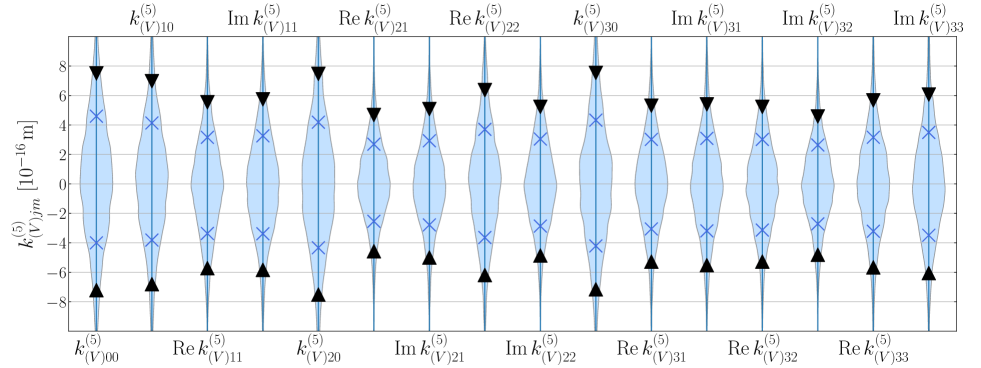
Figure 1: Violin plots of the 16 independent components at mass dimension $d=5$. The 68% and 90% confidence intervals are tagged with “$\times$” and “$\bigtriangleup$” respectively.

Table 1: The 68% confidence intervals of the 16 independent components of $k^{(5)}_{(V)jm}$.

$j$	$m$	Component	Confidence interval $[10^{-16}\,\text{m}]$
0	0	$k^{(5)}_{(V)00}$	$(-4.00,\,4.60)$
1	0	$k^{(5)}_{(V)10}$	$(-3.81,\,4.14)$
1	1	$\text{Re}\,k^{(5)}_{(V)11}$	$(-3.37,\,3.16)$
		$\text{Im}\,k^{(5)}_{(V)11}$	$(-3.38,\,3.26)$
2	0	$k^{(5)}_{(V)20}$	$(-4.34,\,4.19)$
2	1	$\text{Re}\,k^{(5)}_{(V)21}$	$(-2.54,\,2.70)$
		$\text{Im}\,k^{(5)}_{(V)21}$	$(-2.78,\,2.93)$
2	2	$\text{Re}\,k^{(5)}_{(V)22}$	$(-3.64,\,3.70)$
		$\text{Im}\,k^{(5)}_{(V)22}$	$(-2.86,\,3.05)$
3	0	$k^{(5)}_{(V)30}$	$(-4.21,\,4.33)$
3	1	$\text{Re}\,k^{(5)}_{(V)31}$	$(-3.06,\,3.02)$
		$\text{Im}\,k^{(5)}_{(V)31}$	$(-3.19,\,3.09)$
3	2	$\text{Re}\,k^{(5)}_{(V)32}$	$(-3.13,\,3.02)$
		$\text{Im}\,k^{(5)}_{(V)32}$	$(-2.71,\,2.64)$
3	3	$\text{Re}\,k^{(5)}_{(V)33}$	$(-3.22,\,3.16)$
		$\text{Im}\,k^{(5)}_{(V)33}$	$(-3.49,\,3.49)$

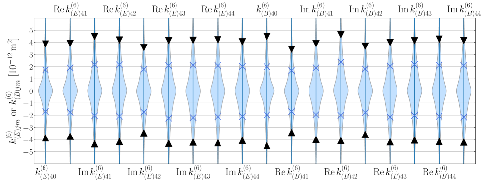
Figure 2: Same as Fig. 1, for mass dimension $d=6$.

Table 2: Same as Table 1, for $k^{(6)}_{(E)jm}$ and $k^{(6)}_{(B)jm}$.

$j$	$m$	Component	Confidence interval $[10^{-12}\,\text{m}^{2}]$
4	0	$k^{(6)}_{(E)40}$	$(-1.70,\,1.73)$
4	1	$\text{Re}\,k^{(6)}_{(E)41}$	$(-1.76,\,1.90)$
		$\text{Im}\,k^{(6)}_{(E)41}$	$(-2.05,\,2.16)$
4	2	$\text{Re}\,k^{(6)}_{(E)42}$	$(-2.08,\,2.15)$
		$\text{Im}\,k^{(6)}_{(E)42}$	$(-1.75,\,1.78)$
4	3	$\text{Re}\,k^{(6)}_{(E)43}$	$(-2.24,\,2.09)$
		$\text{Im}\,k^{(6)}_{(E)43}$	$(-2.19,\,2.11)$
4	4	$\text{Re}\,k^{(6)}_{(E)44}$	$(-2.12,\,2.09)$
		$\text{Im}\,k^{(6)}_{(E)44}$	$(-2.10,\,2.01)$
4	0	$k^{(6)}_{(B)40}$	$(-1.97,\,2.00)$
4	1	$\text{Re}\,k^{(6)}_{(B)41}$	$(-1.70,\,1.67)$
		$\text{Im}\,k^{(6)}_{(B)41}$	$(-1.95,\,1.91)$
4	2	$\text{Re}\,k^{(6)}_{(B)42}$	$(-2.01,\,2.37)$
		$\text{Im}\,k^{(6)}_{(B)42}$	$(-1.78,\,1.81)$
4	3	$\text{Re}\,k^{(6)}_{(B)43}$	$(-2.16,\,2.03)$
		$\text{Im}\,k^{(6)}_{(B)43}$	$(-2.02,\,2.18)$
4	4	$\text{Re}\,k^{(6)}_{(B)44}$	$(-2.09,\,2.12)$
		$\text{Im}\,k^{(6)}_{(B)44}$	$(-2.16,\,2.09)$

First, we take $d=5$ to show how 50 GW events can constrain the coefficient space. For every GW event, based on Eqs. (7–8) we have an inequality of the 16 components, and each inequality gives an area between two hypersurfaces symmetrical about the origin. It is easy to see that $\Delta t$ is actually a linear combination of $k^{(5)}_{(V)jm}$, and the combination coefficients are the spin-weighted spherical harmonics, ${}_{0}Y_{jm}$, which are direction-dependent. Based on the fact that GW events scatter in different sky areas, these linear combinations are expected to be linearly independent. Consequently, the 50 pairs of hypersurfaces can enclose a region containing the origin, where all SME coefficients must be. In this way we have completed a simple but global limitation of the coefficient space. In this closed area every coefficient is bounded. Then we can obtain the value range of each parameter in principle.

To incorporate all uncertainties and statistically obtain the distribution of these SME coefficients, one requires the distribution of the “measured” time delay. As a conservative consideration, we can take the upper bound of $\Delta t$ in Eq. (7) as its standard deviation. Because the violations in SME are expected to be tiny, we take the central value of $\Delta t$ to be zero. We assume that the “measured” time delay obeys a Gaussian normal distribution with $\mu=0$ and $\sigma={1}/({\rho f})$. Based on this, we carry out a global analysis following the steps below.

1. For each GW event, we randomly draw the source parameters in the posterior samples, and calculate the frequency at the amplitude peak.

2. We randomly draw the time delays of the 50 GW events from their respective distributions and take these time delays as the result of one measurement in the Monte Carlo processes.

3. Given the SME coefficients, we calculate the theoretical time delay $\Delta t^{(\text{th})}_{n}$ for the $n$-th GW event where $n$ takes $1,2,\cdots,50$.

4. Considering that the measured time delay obeys a Gaussian distribution with $\mu=\Delta t^{(\text{th})}_{n}$ and $\sigma={1}/({{\rho_{n}}{f_{n}}})$, we construct the multi-Gaussian likelihood as a function of the SME coefficients for all events. After maximizing the likelihood, the corresponding SME coefficients at the extreme point are what we extract from each draw.

5. We repeat steps (i)–(iv) enough times until a stable distribution is obtained.

For the 16 components at $d=5$, the violin plots of the one-dimensional marginalized distributions are given in Fig. 1, while their confidence intervals are given in Table 1. Because the dependence of $\Delta t$ on the SME coefficients is linear, the marginalized distributions are very close to Gaussian distributions. Similar to Shao (2020), no obvious correlation is found among the components due to the different properties of the GW events, including sky locations, peak GW frequencies and so on.

For the 18 components at mass dimension $d=6$, we have to analyze with more care. Since $\varsigma_{(+4)}$ is a complex number, the calculation of $\sqrt{|\varsigma_{(+4)}|^{2}}$ is much more difficult than $d=5$, whereas $\varsigma_{(0)}$ is real and the square root is trivial. Due to this reason, the dependence of $\Delta t$ on the SME coefficients is highly nonlinear, leading the marginalized distributions to be more peaked than the Gaussian distribution in the end. Despite the complications above, correlations between the 18 independent components are still small. Their one-dimensional marginalized distributions are given in Fig. 2 and the 68% confidence intervals are illustrated in Table 2.

V Discussion and summary

Gravitational waves (GWs) provide excellent opportunities to make a profound study of the gravitational Lorentz invariance violation (gLIV). Lots of work (Wang & Zhao, 2020; Nishizawa, 2018; Abbott et al., 2019b; Mirshekari et al., 2012; Wang et al., 2021) have been performed to test the Lorentz symmetry in General Relativity (GR) using GW events. While a general gLIV includes anisotropy, dispersion, and birefringence, previous work mostly emphasized the isotropic birefringent phenomenon.

In our work, we focus on the anisotropic birefringence of GWs in the popular theoretical framework called the standard-model extension (SME; Colladay & Kostelecký, 1997; Kostelecký, 2004). Assuming that gLIV mainly occurs at a particular mass dimension, for the two lowest dimensions that can produce birefringence, $d=5$ and 6, we separately carry out global analysis on them and constrain the whole coefficient space fully. Thanks to the multiple GW events in the GW transient catalogs GWTC-1 and GWTC-2, we completely break the degeneracy among the 16 independent components of the SME coefficients $k^{(5)}_{(V)jm}$ at $d=5$, and 18 independent components at $d=6$. This is reflected in the results of Tables 1 & 2, which are obtained by simultaneously constraining all the coefficients, instead of setting only one coefficient to be nonzero each time (i.e., the “maximum reach” approach; Tasson, 2019). As can be seen, there is no obvious violation of GR in our results, and our limits on the SME coefficients are $2$ to $7$ times tighter than that in the earlier work (Shao, 2020).

While in this paper, we have only made use of one type of phenomena in the birefringent gLIV, namely the differences of the arrival times between two modes, there are many more approaches to improve our tests. First, more information can be extracted from the birefringence phenomena, such as the changes of the polarizations. Similar analysis has been conducted in the photon sector (Kostelecký & Mewes, 2008, 2013). Second, Eq. (7) is a relatively simple estimation of the time delay (Shao, 2020), and in fact Mewes (2019) has worked out the whole deformed waveform analytics and we can use these modified templates to implement the matched-filtering analysis. For mass dimensions $5$ and $6$, the computational cost is expected to be significant (O’Neal-Ault et al., 2021). Third, in a very unlikely scenario, the pattern function of GW detectors might hide one of the two polarizations. However, we think it is impossible to happen in all 50 GW events that we used here. However, to entirely rule out this possibility, one needs to incorporate the polarization of the events, probably in a matched-filtering analysis (Wang et al., 2021; O’Neal-Ault et al., 2021). Finally, advanced detectors like the KAGRA (Aso et al., 2013) have recently joined the global efforts to detect GWs. With the ground-based detector network, more and more GWs in a wider frequency range will obviously bring direct improvements to our results.

In conclusion, the GWs are undoubtedly fantastic phenomena to test fundamental principles in modern physics, and we expect a brighter future in the coming years for the fundamental physics through the use of these treasures of the Nature.

References

- Abbott et al. (2016) Abbott, B. P., et al. 2016, Phys. Rev. Lett., 116, 061102, doi: 10.1103/PhysRevLett.116.061102
- Abbott et al. (2017) —. 2017, Astrophys. J., 848, L13, doi: 10.3847/2041-8213/aa920c
- Abbott et al. (2019a) —. 2019a, Phys. Rev. X, 9, 031040, doi: 10.1103/PhysRevX.9.031040
- Abbott et al. (2019b) —. 2019b, Phys. Rev. D, 100, 104036, doi: 10.1103/PhysRevD.100.104036
- Abbott et al. (2020a) —. 2020a, Astrophys. J. Lett., 892, L3, doi: 10.3847/2041-8213/ab75f5
- Abbott et al. (2020b) Abbott, R., et al. 2020b, Astrophys. J. Lett., 896, L44, doi: 10.3847/2041-8213/ab960f
- Abbott et al. (2021) —. 2021, Phys. Rev. X, 11, 021053, doi: 10.1103/PhysRevX.11.021053
- Aso et al. (2013) Aso, Y., Michimura, Y., Somiya, K., et al. 2013, Phys. Rev. D, 88, 043007, doi: 10.1103/PhysRevD.88.043007
- Bailey et al. (2015) Bailey, Q. G., Kostelecký, V. A., & Xu, R. 2015, Phys. Rev. D, 91, 022006, doi: 10.1103/PhysRevD.91.022006
- Battat et al. (2007) Battat, J. B. R., Chandler, J. F., & Stubbs, C. W. 2007, Phys. Rev. Lett., 99, 241103, doi: 10.1103/PhysRevLett.99.241103
- Bluhm & Kostelecký (2005) Bluhm, R., & Kostelecký, V. A. 2005, Phys. Rev. D, 71, 065008, doi: 10.1103/PhysRevD.71.065008
- Bohé et al. (2017) Bohé, A., et al. 2017, Phys. Rev. D, 95, 044028, doi: 10.1103/PhysRevD.95.044028
- Bourgoin et al. (2017) Bourgoin, A., Le Poncin-Lafitte, C., Hees, A., et al. 2017, Phys. Rev. Lett., 119, 201102, doi: 10.1103/PhysRevLett.119.201102
- Colladay & Kostelecký (1997) Colladay, D., & Kostelecký, V. A. 1997, Phys. Rev. D, 55, 6760, doi: 10.1103/PhysRevD.55.6760
- Hees et al. (2016) Hees, A., Bailey, Q. G., Bourgoin, A., et al. 2016, Universe, 2, 30, doi: 10.3390/universe2040030
- Hees et al. (2015) Hees, A., Bailey, Q. G., Le Poncin-Lafitte, C., et al. 2015, Phys. Rev. D, 92, 064049, doi: 10.1103/PhysRevD.92.064049
- Iorio (2012) Iorio, L. 2012, Class. Quant. Grav., 29, 175007, doi: 10.1088/0264-9381/29/17/175007
- Jennings et al. (2015) Jennings, R. J., Tasson, J. D., & Yang, S. 2015, Phys. Rev. D, 92, 125028, doi: 10.1103/PhysRevD.92.125028
- Kostelecký (2004) Kostelecký, V. A. 2004, Phys. Rev. D, 69, 105009, doi: 10.1103/PhysRevD.69.105009
- Kostelecký & Li (2019) Kostelecký, V. A., & Li, Z. 2019, Phys. Rev. D, 99, 056016, doi: 10.1103/PhysRevD.99.056016
- Kostelecký & Mewes (2002) Kostelecký, V. A., & Mewes, M. 2002, Phys. Rev. D, 66, 056005, doi: 10.1103/PhysRevD.66.056005
- Kostelecký & Mewes (2008) —. 2008, Astrophys. J. Lett., 689, L1, doi: 10.1086/595815
- Kostelecký & Mewes (2009) —. 2009, Phys. Rev. D, 80, 015020, doi: 10.1103/PhysRevD.80.015020
- Kostelecký & Mewes (2013) —. 2013, Phys. Rev. Lett., 110, 201601, doi: 10.1103/PhysRevLett.110.201601
- Kostelecký & Mewes (2016) —. 2016, Phys. Lett. B, 757, 510, doi: 10.1016/j.physletb.2016.04.040
- Kostelecký & Potting (1991) Kostelecký, V. A., & Potting, R. 1991, Nucl. Phys. B, 359, 545, doi: 10.1016/0550-3213(91)90071-5
- Kostelecký & Russell (2011) Kostelecký, V. A., & Russell, N. 2011, Rev. Mod. Phys., 83, 11, doi: 10.1103/RevModPhys.83.11
- Kostelecký & Samuel (1989) Kostelecký, V. A., & Samuel, S. 1989, Phys. Rev. D, 39, 683, doi: 10.1103/PhysRevD.39.683
- Kostelecký & Tasson (2015) Kostelecký, V. A., & Tasson, J. D. 2015, Phys. Lett. B, 749, 551, doi: 10.1016/j.physletb.2015.08.060
- Le Poncin-Lafitte et al. (2016) Le Poncin-Lafitte, C., Hees, A., & Lambert, S. 2016, Phys. Rev. D, 94, 125030, doi: 10.1103/PhysRevD.94.125030
- Mewes (2019) Mewes, M. 2019, Phys. Rev. D, 99, 104062, doi: 10.1103/PhysRevD.99.104062
- Mirshekari et al. (2012) Mirshekari, S., Yunes, N., & Will, C. M. 2012, Phys. Rev. D, 85, 024041, doi: 10.1103/PhysRevD.85.024041
- Mueller et al. (2008) Mueller, H., Chiow, S.-w., Herrmann, S., Chu, S., & Chung, K.-Y. 2008, Phys. Rev. Lett., 100, 031101, doi: 10.1103/PhysRevLett.100.031101
- Nishizawa (2018) Nishizawa, A. 2018, Phys. Rev. D, 97, 104037, doi: 10.1103/PhysRevD.97.104037
- O’Neal-Ault et al. (2021) O’Neal-Ault, K., Bailey, Q. G., Dumerchat, T., Haegel, L., & Tasson, J. 2021. https://arxiv.org/abs/2108.06298
- Schreck (2017) Schreck, M. 2017, Class. Quant. Grav., 34, 135009, doi: 10.1088/1361-6382/aa7074
- Shao et al. (2016) Shao, C.-G., et al. 2016, Phys. Rev. Lett., 117, 071102, doi: 10.1103/PhysRevLett.117.071102
- Shao (2014a) Shao, L. 2014a, Phys. Rev. Lett., 112, 111103, doi: 10.1103/PhysRevLett.112.111103
- Shao (2014b) —. 2014b, Phys. Rev. D, 90, 122009, doi: 10.1103/PhysRevD.90.122009
- Shao (2019) Shao, L. 2019, in Proceedings of the 8th Meeting on CPT and Lorentz Symmetry, doi: 10.1142/9789811213984_0043, arXiv:1905.08405
- Shao (2020) —. 2020, Phys. Rev. D, 101, 104019, doi: 10.1103/PhysRevD.101.104019
- Shao & Bailey (2018) Shao, L., & Bailey, Q. G. 2018, Phys. Rev. D, 98, 084049, doi: 10.1103/PhysRevD.98.084049
- Shao & Bailey (2019) —. 2019, Phys. Rev. D, 99, 084017, doi: 10.1103/PhysRevD.99.084017
- Shao & Wex (2016) Shao, L., & Wex, N. 2016, Sci. China Phys. Mech. Astron., 59, 699501, doi: 10.1007/s11433-016-0087-6
- Tasson (2019) Tasson, J. D. 2019, in Proceedings of the 8th Meeting on CPT and Lorentz Symmetry, doi: 10.1142/9789811213984_0004
- Wang & Zhao (2020) Wang, S., & Zhao, Z.-C. 2020, Eur. Phys. J. C, 80, 1032, doi: 10.1140/epjc/s10052-020-08628-x
- Wang et al. (2021) Wang, Y.-F., Niu, R., Zhu, T., & Zhao, W. 2021, Astrophys. J., 908, 58, doi: 10.3847/1538-4357/abd7a6