A well balanced finite volume scheme for
general relativity

Abstract

In this work we present a novel second order accurate well balanced (WB) finite volume (FV) scheme for the solution of the general relativistic magnetohydrodynamics (GRMHD) equations and the first order CCZ4 formulation (FO-CCZ4) of the Einstein field equations of general relativity, as well as the fully coupled FO-CCZ4 + GRMHD system. These systems of first order hyperbolic PDEs allow to study the dynamics of the matter and the dynamics of the space-time according to the theory of general relativity.

The new well balanced finite volume scheme presented here exploits the knowledge of an equilibrium solution of interest when integrating the conservative fluxes, the nonconservative products and the algebraic source terms, and also when performing the piecewise linear data reconstruction. This results in a rather simple modification of the underlying second order FV scheme, which, however, being able to cancel numerical errors committed with respect to the equilibrium component of the numerical solution, substantially improves the accuracy and long-time stability of the numerical scheme when simulating small perturbations of stationary equilibria. In particular, the need for well balanced techniques appears to be more and more crucial as the applications increase their complexity. We close the paper with a series of numerical tests of increasing difficulty, where we study the evolution of small perturbations of accretion problems and stable TOV neutron stars. Our results show that the well balancing significantly improves the long-time stability of the finite volume scheme compared to a standard one.

35L40, 65M08, 83C05, 83C10, 85-08, 85-10, 85A30.

1 Introduction

The main goal of this work is to improve the long-term stability and accuracy of finite volume schemes in the context of numerical general relativity. The models that we consider here are the general relativistic Euler and magnetohydrodynamics (GRMHD) equations [17, 6, 11, 48, 49, 57] and the so-called first order CCZ4 formulation (FO-CCZ4) of the Einstein field equations [3, 55, 54]. The governing PDE systems in general relativity are extremely challenging since they contain not only very complex equations with many unknowns, but some systems are also subject to involution constraints that affect hyperbolicity and thus well-posedness of the initial value problem. Moreover, the applications of interest in this field, such as the evolution of accretion disks, neutron stars and black holes, are characterized by a disparity of the involved space and time scales: indeed, we need to observe the long time evolution of phenomena developing over astronomical distances, such as gravitational waves, but whose behavior is strongly affected by physical perturbations developed at smaller scales like a binary neutron star system. Furthermore, it is particularly challenging to simulate small perturbations of stationary equilibria when the perturbations are of the order of the numerical discretization error. Hence, the main objective of this paper consists in improving long-time stability and accuracy of numerical methods for the simulation of astrophysical phenomena occurring close to stationary equilibrium solutions of the GRMHD and FO-CCZ4 equations. This will be achieved thanks to the introduction of modern well balancing (WB) techniques (see for example [23, 74, 38, 39, 62, 40] and the references therein) inside the finite volume scheme that allow to preserve given equilibria of the governing PDE system exactly at the discrete level, thus avoiding that small physical perturbations are masked by numerical discretization errors. To the best of our knowledge, this is the very first time that an exactly well balanced finite volume scheme is proposed for the GRMHD and FO-CCZ4 equations of numerical general relativity, for a given set of relevant stationary solutions.

A brief literature review on the state of the art of numerical general relativity as well as on existing well balanced techniques for computational fluid dynamics in the context of free surface shallow water flows and the Euler equations of gasdynamics with Newtonian gravity is given below.

The GRMHD model combines the fluid description of matter with a simplified theory for electromagnetic fields in the absence of free charge carriers. It was studied for the first time in [100, 9, 87] and [8], without and with electromagnetic fields. Substantial progress in the field has been made by the group of Ibañez and co-workers, who introduced the now universally adopted Valencia formulation of general relativistic hydrodynamics and magnetohydrodynamics, see e.g. [17, 11, 58, 75] and references therein. There, the GRHD and GRMHD systems have been cast into conservation law form, which allowed to apply classical Godunov-type finite volume schemes for hyperbolic equations. Subsequently, many different solvers have been developed, see for example [16, 52, 10, 49, 65, 7, 71, 31, 83, 51, 84, 99, 82]. Other studies incorporate radiation transfer, like the one proposed by [91], or include the full Maxwell theory in a resistive relativistic MHD formulation [79, 56, 51, 32, 33, 5]. Here we follow the approach of [57], where the gravitational field in fixed background space–time (Cowling approximation) are treated via the use of nonconservative products instead of the usually employed algebraic source terms, since gravity terms can be expressed as functions of the spatial derivatives of the lapse, the shift vector and the spatial metric tensor, i.e. some of the conserved variables.

Besides the evolution of the matter, the numerical integration of the Einstein field equations for the time evolution of the metric is another challenging problem. The covariant nature of the equations allows the choice of arbitrary moving curvilinear coordinates (gauge freedom), and hence first a suitable set of space-time coordinates must be chosen. The first step in this direction was achieved with the 3+1 (space + time) ADM formulation of [12], see also [13, 20], which allowed to rewrite the Einstein field equations as an initial boundary value problem, but the proposed PDE system was not hyperbolic. A mixed elliptic-hyperbolic formalism, know as fully constrained formulation (FCF) was then proposed in [28] and its mathematical structure, well-posedness and uniqueness were further analyzed in [46, 45]. Then, among the first hyperbolic formulations was the BSSNOK (Baumgarte-Shapiro-Shibata-Nakamura-Oohara-Kojima) formulation [89, 19, 77]. Subsequently, different alternative formulations were proposed, like the Z4 formulation [25, 26, 2], the Z4c system [24] and the CCZ4 in [3, 4]. For an exhaustive overview of different models used in numerical general relativity, see [1]. Most of the previous formulations led to first order systems in time, but with first and second order derivatives in space, and were therefore not directly accessible for standard Godunov-type methods for first order hyperbolic systems. Instead, the systems were typically integrated with high order central finite difference schemes. The problem of hyperbolicity of different second order in space formulations of general relativity was discussed in [68]. The PDE system used in this paper is based on the first order CCZ4 formulation (FO-CCZ4) that has been derived in [55] and for which strong hyperbolicity has been demonstrated for a particular choice of gauges. In [54], the curl-free condition of certain evolution variables of the FO-CCZ4 system was taken into account via a novel hyperbolic generalized Lagrangian multiplier (GLM) curl-cleaning technique.

Numerical simulations of GRMHD and FO-CCZ4 at the aid of high order DG schemes with a posteriori subcell finite volume limiter have been presented in [57, 55, 54], showing the appropriateness of the chosen governing PDE systems and the numerical methods employed for their solution. However, the obtained results also clearly indicate that with standard schemes for hyperbolic PDE one can reach only rather short simulation times (w.r.t astrophysical timescales) and rather fine meshes (w.r.t astrophysical spatial scales) are required, even for the simulation of stationary equilibrium solutions of the governing PDE systems. Thus, there is a necessity to endow existing methods with the ability of preserving additional physical properties of the underlying PDE system in such a way that spurious numerical modes can be eliminated, numerical dissipation reduced and small-scale structures can manifest inside large-scale macroscopic models. In Newtonian computational fluid dynamics, such improved properties of a numerical scheme can be achieved at the aid of well balancing (WB), which allows to preserve certain stationary equilibrium solutions of the governing PDE system exactly at the discrete level. In the pioneering work of Bermúdez and Vázquez in 1994 [23] the authors have proposed an exactly well balanced Roe solver for lake at rest solutions of the shallow water equations. Further important results in this field have been achieved in [30, 15, 85, 38, 66, 74, 81, 92, 39]. More recent works are, for example, [64, 61, 42, 21, 40, 14]. Since it is impossible to mention all the relevant references here, we refer to the recent review paper [40], which besides an interesting treatment of discontinuous equilibria contains a rather complete review of the wide literature on well balanced schemes. Finally, we would like to underline that the development of WB and structure preserving schemes for astrophysical applications is a topic of growing interest, although the existing works so far only employ much simpler Newtonian PDE systems, see for example [29, 69, 70, 41, 88, 50, 22, 62, 72, 67, 93] and the references therein, where well balanced schemes for the Euler equations of gasdynamics with Newtonian gravity were proposed.

The rest of the paper is organized as follows. In Section 2 we introduce the governing PDE systems that are solved in this paper; in Section 3 we present our new well balanced second order finite volume scheme for numerical general relativity that allows to preserve smooth equilibria exactly at the discrete level. The increased stability and resolution gained with the use of the new scheme are shown via a series of numerical tests of increasing difficulty presented in Section 4. We close the paper with some remarks and an outlook to future works in Section 5.

2 Governing PDE systems

All governing PDE systems for numerical general relativity used throughout this paper can be written as first order hyperbolic partial differential equations of the following general form:

(1) $$\mathbf{Q}_{t}+\nabla\cdot\mathbf{F}(\mathbf{Q})+\mathbf{B}(\mathbf{Q})\cdot\nabla\mathbf{Q}=\mathbf{S}(\mathbf{Q}),\quad\mathbf{x}=(x_{1},x_{2},x_{3})\in\Omega\subset\mathbb{R}^{3},$$

where $\mathbf{x}=(x_{1},x_{2},x_{3})=(x,y,z)$ is the spatial position vector, $t$ represents the time, $\Omega$ is the computational domain, $\mathbf{Q}=(q_{1},q_{2},\dots,q_{m})^{T}$ is the state vector defined in the space of the admissible states $\Omega_{\mathbf{Q}}\subset\mathbb{R}^{m}$, $\mathbf{F}(\mathbf{Q})=(\mathbf{f}(\mathbf{Q}),\mathbf{g}(\mathbf{Q}),\mathbf{h}(\mathbf{Q}))$ is the non linear flux tensor, $\mathbf{B}(\mathbf{Q})=(\mathbf{B}_{1}(\mathbf{Q}),\mathbf{B}_{2}(\mathbf{Q}),\mathbf{B}_{3}(\mathbf{Q}))$ is a matrix collecting the nonconservative terms, and $\mathbf{S}(\mathbf{Q})$ represents a nonlinear algebraic source term. The form (1) is said to be hyperbolic if for all directions $\mathbf{n}\neq\mathbf{0}$ the matrix $\mathbf{A}_{n}=\left(\partial\mathbf{F}/\partial{\mathbf{Q}}+\mathbf{B}(\mathbf{Q})\right)\cdot\mathbf{n}$ has $m$ real eigenvalues and a full set of $m$ linearly independent eigenvectors.

In this work we will consider problems that, due to their spherical symmetry, can be written as one-dimensional hyperbolic PDE systems of the type

(2) $$\mathbf{Q}_{t}+\mathbf{f}_{x}(\mathbf{Q})+\mathbf{B}_{1}(\mathbf{Q})\cdot\mathbf{Q}_{x}=\mathbf{S}(\mathbf{Q})-\mathbf{S_{b}}(\mathbf{Q},\mathbf{Q}_{y},\mathbf{Q}_{z}),$$

where in $\mathbf{S_{b}}$ we collect eventual non-zero terms depending on derivatives of the state variables with respect to the $y$ and $z$ coordinates. Throughout this paper we employ the Einstein summation convention, which implies summation over two repeated indices and we use Greek letters for four-dimensional indices running from 0 to 3 and Latin letters for three-dimensional indices running from 1 to 3. We work in a geometrized set of units, in which the speed of light and the gravitational constant are set to unity, i.e. $c=G=1$.

The complete set of governing equations of the fully coupled FO-CCZ4 + GRMHD system reads as follows (see [55, 54] and [57]):

(3a) $$\partial_{t}\tilde{\gamma}_{ij} = {\beta^{k}2D_{kij}+\tilde{\gamma}_{ki}B_{j}^{k}+\tilde{\gamma}_{kj}B_{i}^{k}-\frac{2}{3}\tilde{\gamma}_{ij}B_{k}^{k}}-2\alpha\left(\tilde{A}_{ij}-{\frac{1}{3}\tilde{\gamma}_{ij}{\rm tr}{\tilde{A}}}\right),$$

(3b) $${\partial_{t}\ln{\alpha}} = {\beta^{k}A_{k}}-\alpha g(\alpha)(K-K_{0}-2\Theta{c}),\qquad\qquad\partial_{t}K_{0}=0,$$

(3c) $$\partial_{t}\beta^{i} = s\beta^{k}B_{k}^{i}+sfb^{i},$$

(3d) $${\partial_{t}\ln{\phi}} = {\beta^{k}P_{k}}+\frac{1}{3}\left(\alpha K-{B_{k}^{k}}\right),$$

$$\partial_{t}\tilde{A}_{ij}-\beta^{k}\partial_{k}\tilde{A}_{ij}+\phi^{2}\bigg{[}\nabla_{i}\nabla_{j}\alpha-\alpha\left(R_{ij}+\nabla_{i}Z_{j}+\nabla_{j}Z_{i}-8\pi S_{ij}\right)\bigg{]}$$

$$-\frac{1}{3}\tilde{\gamma}_{ij}\bigg{[}\nabla^{k}\nabla_{k}\alpha-\alpha(R+2\nabla_{k}Z^{k}-8\pi S)\bigg{]}$$

(4a) $$={\tilde{A}_{ki}B_{j}^{k}+\tilde{A}_{kj}B_{i}^{k}-\frac{2}{3}\tilde{A}_{ij}B_{k}^{k}}+\alpha\tilde{A}_{ij}(K-2\Theta{c})-2\alpha\tilde{A}_{il}\tilde{\gamma}^{lm}\tilde{A}_{mj},\$$

$$\partial_{t}K-\beta^{k}\partial_{k}K+\nabla^{i}\nabla_{i}\alpha-\alpha(R+2\nabla_{i}Z^{i})$$

(4b) $$=\alpha K(K-2\Theta{c})-3\alpha\kappa_{1}(1+\kappa_{2})\Theta+4\pi\alpha(S-3\tau),\$$

$$\partial_{t}\Theta-\beta^{k}\partial_{k}\Theta-\frac{1}{2}\alpha{e^{2}}(R+2\nabla_{i}Z^{i})$$

(4c) $$=\alpha{e^{2}}\left(\frac{1}{3}K^{2}-\frac{1}{2}\tilde{A}_{ij}\tilde{A}^{ij}-8\pi\tau\right)-\alpha\Theta K{c}-{Z^{i}\alpha A_{i}}-\alpha\kappa_{1}(2+\kappa_{2})\Theta,\$$

$$\partial_{t}\hat{\Gamma}^{i}-\beta^{k}\partial_{k}\hat{\Gamma}^{i}+\frac{4}{3}\alpha\tilde{\gamma}^{ij}\partial_{j}K-\tilde{\gamma}^{kl}\partial_{(k}B_{l)}^{i}-\tilde{\gamma}^{ik}\left(\frac{1}{3}\partial_{(k}B_{l)}^{l}+{s2\alpha\tilde{\gamma}^{nm}\partial_{k}\tilde{A}_{nm}}+2\alpha\partial_{k}\Theta\right)$$

$$={\frac{2}{3}\tilde{\Gamma}^{i}B_{k}^{k}-\tilde{\Gamma}^{k}B_{k}^{i}}+2\alpha\left(\tilde{\Gamma}^{i}_{jk}\tilde{A}^{jk}-3\tilde{A}^{ij}P_{j}\right)-2\alpha\tilde{\gamma}^{ki}\left(\Theta A_{k}+\frac{2}{3}KZ_{k}\right)-2\alpha\tilde{A}^{ij}A_{j}$$

$$-{4s\,\alpha\tilde{\gamma}^{ik}D_{k}^{~{}\,nm}\tilde{A}_{nm}}+2\kappa_{3}\left(\frac{2}{3}\tilde{\gamma}^{ij}Z_{j}B_{k}^{k}-\tilde{\gamma}^{jk}Z_{j}B_{k}^{i}\right)-2\alpha\kappa_{1}\tilde{\gamma}^{ij}Z_{j}-16\pi\alpha\tilde{\gamma}^{ij}S_{j},$$

(4d)

(4e) $$\partial_{t}b^{i}-s\beta^{k}\partial_{k}b^{i}=s\left(\partial_{t}\hat{\Gamma}^{i}-\beta^{k}\partial_{k}\hat{\Gamma}^{i}-\eta b^{i}\right).$$

The use of the logarithms in the evolution equations for the lapse and the conformal factor is for convenience, in order to always guarantee positivity of $\alpha$ and $\phi$ also at the discrete level. In order to obtain a strongly hyperbolic first-order reduction, the following evolution system for the auxiliary variables $A_{k}:=\partial_{k}\alpha/\alpha$, $B_{k}^{i}:=\partial_{k}\beta^{i}$, $D_{kij}:=\frac{1}{2}\partial_{k}\tilde{\gamma}_{ij}$ and $P_{k}:=\partial_{k}\phi/\phi$ is added, accounting also for the stationary involutions of the governing PDE system:

$$\partial_{t}A_{k}-{\beta^{l}\partial_{l}A_{k}}+\alpha g(\alpha)\left(\partial_{k}K-\partial_{k}K_{0}-2c\partial_{k}\Theta\right)+{s\alpha g(\alpha)\tilde{\gamma}^{nm}\partial_{k}\tilde{A}_{nm}}$$

(5a) $$=+{2s\,\alpha g(\alpha)D_{k}^{~{}\,nm}\tilde{A}_{nm}}-\alpha A_{k}\left(K-K_{0}-2\Theta c\right)h(\alpha)+B_{k}^{l}~{}A_{l}\,,$$

$$\partial_{t}B_{k}^{i}-s\beta^{l}\partial_{l}B_{k}^{i}-s\left(f\partial_{k}b^{i}-\alpha^{2}\mu\,\tilde{\gamma}^{ij}\left(\partial_{k}P_{j}-\partial_{j}P_{k}\right)\right)$$

(5b) $$-s\left(\alpha^{2}\mu\,\tilde{\gamma}^{ij}\tilde{\gamma}^{nl}\left(\partial_{k}D_{ljn}-\partial_{l}D_{kjn}\right)\right)=sB^{l}_{k}~{}B^{i}_{l},$$

$$\partial_{t}D_{kij}-{\beta^{l}\partial_{l}D_{kij}}+s\left(-\frac{1}{2}\tilde{\gamma}_{mi}\partial_{(k}{B}_{j)}^{m}-\frac{1}{2}\tilde{\gamma}_{mj}\partial_{(k}{B}_{i)}^{m}+\frac{1}{3}\tilde{\gamma}_{ij}\partial_{(k}{B}_{m)}^{m}\right)$$

$$+\alpha\partial_{k}\tilde{A}_{ij}-{\alpha\frac{1}{3}\tilde{\gamma}_{ij}\tilde{\gamma}^{nm}\partial_{k}\tilde{A}_{nm}}=B_{k}^{l}D_{lij}+B_{j}^{l}D_{kli}+B_{i}^{l}D_{klj}-\frac{2}{3}B_{l}^{l}D_{kij}$$

(5c) $$-\alpha\frac{2}{3}\tilde{\gamma}_{ij}D_{k}^{~{}\,nm}\tilde{A}_{nm}-\alpha A_{k}\left(\tilde{A}_{ij}-\frac{1}{3}\tilde{\gamma}_{ij}{\rm tr}\tilde{A}\right),$$

$$\partial_{t}P_{k}-\beta^{l}\partial_{l}P_{k}-\frac{1}{3}\alpha\partial_{k}K+\frac{1}{3}\partial_{(k}{B}_{i)}^{i}-{s\frac{1}{3}\alpha\tilde{\gamma}^{nm}\partial_{k}\tilde{A}_{nm}}$$

(5d) $$=\frac{1}{3}\alpha A_{k}K+B_{k}^{l}P_{l}-{s\frac{2}{3}\alpha\,D_{k}^{~{}\,nm}\tilde{A}_{nm}}.$$

The matter and magnetic field evolution equations, which are fully coupled with the above FO-CCZ4 system read:

(6) $$\partial_{t}(\sqrt{\gamma}D)+\partial_{i}\left(\gamma^{\frac{1}{2}}\left(\alpha v^{i}D-\beta^{i}D\right)\right) = 0,$$

$$\partial_{t}(\sqrt{\gamma}S_{j})+\partial_{i}\left(\gamma^{\frac{1}{2}}\left(\alpha T^{i}_{j}-\beta^{i}S_{j}\right)\right)$$

(7) $$=\gamma^{\frac{1}{2}}\left(\alpha T^{ik}C_{jik}+S_{i}B_{j}^{i}-\alpha\tau A_{j}\right),$$

$$\partial_{t}(\sqrt{\gamma}\tau)+\partial_{i}\left(\gamma^{\frac{1}{2}}\left(\alpha\left(S^{i}-v^{i}D\right)-\beta^{i}\tau\right)\right)$$

(8) $$=\gamma^{\frac{1}{2}}\left(\alpha K_{ij}T^{ij}-\alpha S^{j}A_{j}\right),$$

(9) $$\partial_{t}(\sqrt{\gamma}B^{j})+\partial_{i}\left(\gamma^{\frac{1}{2}}\left(\left(\alpha v^{i}-\beta^{i}\right)B^{j}-\left(\alpha v^{j}-\beta^{j}\right)B^{i}+\varphi\delta^{ij}\right)\right) = 0,$$

(10) $$\partial_{t}(\sqrt{\gamma}\varphi)+\partial_{i}\left(\gamma^{\frac{1}{2}}\left(\alpha c_{h}^{2}B^{i}-\beta^{i}\varphi\right)\right) = 0,$$

with the abbreviation $C_{kij}=\frac{1}{\phi^{2}}\left(D_{kij}-P_{k}\tilde{\gamma}_{ij}\right)$ and where $T^{ij}$ denotes the spatial stress-energy tensor

(11) $$T^{ij} :=\rho hW^{2}{v^{i}v^{j}}-{E^{i}E^{j}}-{B^{i}B^{j}}+\left[p+\frac{1}{2}\left(E^{2}+B^{2}\right)\right]\gamma^{ij}$$

$$={S^{i}v^{j}}+p_{\text{tot}}\gamma^{ij}-\frac{{B^{i}B^{j}}}{W^{2}}-({B}_{k}{v}^{k}){v^{i}B^{j}}\,,$$

with the enthalpy $\rho h=\rho+\frac{\gamma}{\gamma-1}p$, the total pressure defined as

(12) $$p_{\text{tot}}=p+p_{\text{mag}}=p+\frac{1}{2}\left[B^{2}/W^{2}+(B\cdot v)^{2}\right]\,.$$

The governing PDE system (3a)–(5) contains the terms defined below:

$${\rm tr}\tilde{A} = \tilde{\gamma}^{ij}\tilde{A}_{ij},\qquad\textnormal{ and }\qquad\tilde{\gamma}=\textnormal{det}(\tilde{\gamma}_{ij}),$$

$$\partial_{k}\tilde{\gamma}^{ij} = -2\tilde{\gamma}^{in}\tilde{\gamma}^{mj}D_{knm}:=-2D_{k}^{~{}\,ij},$$

$$\tilde{\Gamma}_{ij}^{k} = \tilde{\gamma}^{kl}\left(D_{ijl}+D_{jil}-D_{lij}\right),$$

$$\partial_{k}\tilde{\Gamma}_{ij}^{m} = -2D_{k}^{ml}\left(D_{ijl}+D_{jil}-D_{lij}\right)+\tilde{\gamma}^{ml}\left(\partial_{(k}{D}_{i)jl}+\partial_{(k}{D}_{j)il}-\partial_{(k}{D}_{l)ij}\right),$$

$$\Gamma_{ij}^{k} = \tilde{\gamma}^{kl}\left(D_{ijl}+D_{jil}-D_{lij}\right)-\tilde{\gamma}^{kl}\left(\tilde{\gamma}_{jl}P_{i}+\tilde{\gamma}_{il}P_{j}-\tilde{\gamma}_{ij}P_{l}\right)$$

$$= \tilde{\Gamma}_{ij}^{k}-\tilde{\gamma}^{kl}\left(\tilde{\gamma}_{jl}P_{i}+\tilde{\gamma}_{il}P_{j}-\tilde{\gamma}_{ij}P_{l}\right),$$

$$\partial_{k}\Gamma_{ij}^{m} = -2D_{k}^{ml}\left(D_{ijl}+D_{jil}-D_{lij}\right)+2D_{k}^{ml}\left(\tilde{\gamma}_{jl}P_{i}+\tilde{\gamma}_{il}P_{j}-\tilde{\gamma}_{ij}P_{l}\right)$$

$$-2\tilde{\gamma}^{ml}\left(D_{kjl}P_{i}+D_{kil}P_{j}-D_{kij}P_{l}\right)$$

$$+\tilde{\gamma}^{ml}\left(\partial_{(k}{D}_{i)jl}+\partial_{(k}{D}_{j)il}-\partial_{(k}{D}_{l)ij}\right)$$

$$-\tilde{\gamma}^{ml}\left(\tilde{\gamma}_{jl}\partial_{(k}{P}_{i)}+\tilde{\gamma}_{il}\partial_{(k}{P}_{j)}-\tilde{\gamma}_{ij}\partial_{(k}{P}_{l)}\right),$$

$$R^{m}_{ikj} = \partial_{k}\Gamma^{m}_{ij}-\partial_{j}\Gamma^{m}_{ik}+\Gamma^{l}_{ij}\Gamma^{m}_{lk}-\Gamma^{l}_{ik}\Gamma^{m}_{lj},\qquad R_{ij}=R^{m}_{imj},$$

$$\nabla_{i}\nabla_{j}\alpha = \alpha A_{i}A_{j}-\alpha\Gamma^{k}_{ij}A_{k}+\alpha\partial_{(i}{A}_{j)},\qquad\nabla^{i}\nabla_{i}\alpha=\phi^{2}\tilde{\gamma}^{ij}\left(\nabla_{i}\nabla_{j}\alpha\right),$$

$$\tilde{\Gamma}^{i} = \tilde{\gamma}^{jl}\tilde{\Gamma}^{i}_{jl},$$

$$\partial_{k}\tilde{\Gamma}^{i} = -2D_{k}^{jl}\,\tilde{\Gamma}^{i}_{jl}+\tilde{\gamma}^{jl}\,\partial_{k}\tilde{\Gamma}^{i}_{jl},$$

$$Z_{i} = \frac{1}{2}\tilde{\gamma}_{ij}\left(\hat{\Gamma}^{j}-\tilde{\Gamma}^{j}\right),\qquad Z^{i}=\frac{1}{2}\phi^{2}(\hat{\Gamma}^{i}-\tilde{\Gamma}^{i}),$$

$$\nabla_{i}Z_{j} = D_{ijl}\left(\hat{\Gamma}^{l}-\tilde{\Gamma}^{l}\right)+\frac{1}{2}\tilde{\gamma}_{jl}\left(\partial_{i}\hat{\Gamma}^{l}-\partial_{i}\tilde{\Gamma}^{l}\right)-\Gamma^{l}_{ij}Z_{l},$$

$$R+2\nabla_{k}Z^{k} = \phi^{2}\tilde{\gamma}^{ij}\left(R_{ij}+\nabla_{i}Z_{j}+\nabla_{j}Z_{i}\right)\,,$$

$$h(\alpha) = \left(g(\alpha)+\alpha\frac{\partial g(\alpha)}{\partial\alpha}\right).$$

The function $g(\alpha)$ in the PDE for the lapse $\alpha$ controls the slicing condition, where $g(\alpha)=1$ leads to harmonic slicing and $g(\alpha)=2/\alpha$ leads to the so-called $1+\log$ slicing condition, see [27]. As already mentioned above, the auxiliary quantities $A_{k}$, $P_{k}$, $B^{i}_{k}$ and $D_{kij}$ are defined as (scaled) spatial gradients of the primary variables $\alpha$, $\phi$, $\beta^{i}$ and $\tilde{\gamma}_{ij}$, respectively, and read:

(13) $$A_{i}:=\partial_{i}\ln\alpha=\frac{\partial_{i}\alpha}{\alpha},\quad B_{k}^{i}:=\partial_{k}\beta^{i},\quad D_{kij}:=\frac{1}{2}\partial_{k}\tilde{\gamma}_{ij},\quad P_{i}:=\partial_{i}\ln\phi=\frac{\partial_{i}\phi}{\phi}.$$

Hence, as a result, they must satisfy the following curl involutions or so-called second-order ordering constraints [2, 68]:

$$\mathcal{A}_{lk} :=\partial_{l}A_{k}-\partial_{k}A_{l}=0, \mathcal{P}_{lk} :=\partial_{l}P_{k}-\partial_{k}P_{l}=0,$$

(14) $$\mathcal{B}_{lk}^{i} :=\partial_{l}B_{k}^{i}-\partial_{k}B_{l}^{i}=0, \mathcal{D}_{lkij} :=\partial_{l}D_{kij}-\partial_{k}D_{lij}=0.$$

In the governing PDE system above, we have already made use of these curl involutions by symmetrizing the spatial derivatives of the auxiliary variables as follows:

(15) $$\partial_{(k}{A}_{i)}:=\frac{\partial_{k}A_{i}+\partial_{i}A_{k}}{2},\quad\partial_{(k}{P}_{i)}:=\frac{\partial_{k}P_{i}+\partial_{i}P_{k}}{2},\quad$$

(16) $$\partial_{(k}{B}^{i}_{j)}:=\frac{\partial_{k}B^{i}_{j}+\partial_{j}B^{i}_{k}}{2},\quad\partial_{(k}{D}_{l)ij}:=\frac{\partial_{k}D_{lij}+\partial_{l}D_{kij}}{2}.$$

3 Numerical method

In this section, we first briefly recall the standard (not well balanced) second order MUSCL-Hancock scheme applied to (2) and then present the novel well balanced second order finite volume scheme. Throughout this paper, we assume that the equilibria to be preserved are smooth. In other words, equilibria with jumps at the element interfaces are not admitted.

The one-dimensional computational domain $\Omega=[x_{L},x_{R}]$ is covered with $N$ uniform segment elements of length $\Delta x=(x_{R}-x_{L})/N$ denoted by $\Omega_{i}=[x_{i-1/2},x_{i+1/2}]$, $i=1,\dots,N$. The data at time $t^{n}$ are represented by the usual cell averages $\mathbf{Q}_{i}^{n}$

(17) $$\mathbf{Q}_{i}^{n}=\frac{1}{\Delta x}\int_{\Omega_{i}}\mathbf{Q}(x,t^{n})\,dx.$$

3.1 Standard second-order MUSCL-Hancock-type scheme

In the context of standard MUSCL-Hancock-type second order FV schemes [95] for PDE (2) the cell averages $\mathbf{Q}_{i}^{n}$ are evolved in time from $t^{n}$ up to $t^{n+1}=t^{n}+\Delta t$ through

(18) $$\mathbf{Q}_{i}^{n+1}=\mathbf{Q}_{i}^{n}- \frac{\Delta t}{\Delta x}\left(\mathcal{F}_{i+\frac{1}{2}}\left(\mathbf{q}_{i+\frac{1}{2}}^{-},\mathbf{q}_{i+\frac{1}{2}}^{+}\right)-\mathcal{F}_{i-\frac{1}{2}}\left(\mathbf{q}_{i-\frac{1}{2}}^{-},\mathbf{q}_{i-\frac{1}{2}}^{+}\right)\right)$$

$$- \frac{\Delta t}{\Delta x}\left(\mathcal{D}_{i-\frac{1}{2}}\left(\mathbf{q}_{i-\frac{1}{2}}^{-},\mathbf{q}_{i-\frac{1}{2}}^{+}\right)+\mathcal{D}_{i+\frac{1}{2}}\left(\mathbf{q}_{i+\frac{1}{2}}^{-},\mathbf{q}_{i+\frac{1}{2}}^{+}\right)\right)$$

$$- {\Delta t}\,\mathbf{B}\left(\mathbf{q}_{i}^{n+\frac{1}{2}}\right)\cdot\partial_{x}\mathbf{Q}_{i}^{n}+{\Delta t}\,\mathbf{S}\left(\mathbf{q}_{i}^{n+\frac{1}{2}}\right)-{\Delta t}\,\mathbf{S_{b}}\left(\mathbf{q}_{i}^{n+\frac{1}{2}},\partial_{y}\mathbf{Q}_{i},\partial_{z}\mathbf{Q}_{i}\right).$$

In (18), $\mathcal{F}_{i\pm\frac{1}{2}}$ represent the numerical fluxes and the $\mathcal{D}_{i\pm\frac{1}{2}}$ are the nonconservative jump terms of (1) at the element interfaces given respectively by

(19) $$\mathcal{F}(\mathbf{q}^{-},\mathbf{q}^{+})=\ \frac{1}{2}\left(\mathbf{f}(\mathbf{q}^{+})+\mathbf{f}(\mathbf{q}^{-})\right)-\frac{1}{2}s_{\max}\left(\mathbf{q}^{+}-\mathbf{q}^{-}\right)$$

and

(20) $$\mathcal{D}(\mathbf{q}^{-},\mathbf{q}^{+})=\frac{1}{2}\left(\int\limits_{0}^{1}{\mathbf{B}_{1}}\left(\mathbf{\Psi}(\mathbf{q}^{-},\mathbf{q}^{+},\tau)\right)\,ds\right)\cdot\left(\mathbf{q}^{+}-\mathbf{q}^{-}\right)\!.$$

In our scheme we employ a simple Rusanov-type Riemann solver, where $s_{\max}$ is the maximum eigenvalue of the system matrices $\mathbf{A}(\mathbf{q}^{+})$ and $\mathbf{A}(\mathbf{q}^{-})$, and the theory introduced in [47] is used for integrating the nonconservative products along a Lipschitz continuous path $\mathbf{\Psi}(\mathbf{q}^{-},\mathbf{q}^{+},s)$ with $0\leq s\leq 1$, $\mathbf{\Psi}(\mathbf{q}^{-},\mathbf{q}^{+},0)=\mathbf{q}^{-}$ and $\mathbf{\Psi}(\mathbf{q}^{-},\mathbf{q}^{+},1)=\mathbf{q}^{+}$. Throughout this paper we employ the simple straight-line segment path

(21) $$\mathbf{\Psi}(\mathbf{q}^{-},\mathbf{q}^{+},s)=\mathbf{q}^{-}+s\left(\mathbf{q}^{+}-\mathbf{q}^{-}\right)\!,\qquad s\in[0,1].$$

Moreover, in (18) the values

(22) $$\mathbf{q}_{i-\frac{1}{2}}^{+}=\mathbf{q}_{i}^{n}(x_{i-\frac{1}{2}},t^{n+\frac{1}{2}}),\ \ \mathbf{q}_{i+\frac{1}{2}}^{-}=\mathbf{q}_{i}^{n}(x_{i+\frac{1}{2}},t^{n+\frac{1}{2}}),\ \ \mathbf{q}_{i}^{n+\frac{1}{2}}=\mathbf{q}_{i}^{n}(x_{i},t^{n+\frac{1}{2}}),$$

represent the evaluation of the reconstruction polynomials $\mathbf{q}_{i}^{n}(x,t)$ respectively at the two boundaries $x_{i\pm 1/2}$ and in the barycenter $x_{i}$ of $\Omega_{i}$ at the time-midpoint of $[t^{n},t^{n+1}]$ called $t^{n+1/2}$. The reconstruction polynomial $\mathbf{q}_{i}^{n}(x,t)$ is computed through the MUSCL-Hancock strategy, see [96, 97, 95], in conjunction with the minmod slope limiter. Thus we write it in the form of a linear polynomial in space and time that reads

(23) $$\mathbf{q}_{i}^{n}(x,t)=\mathbf{w}_{i}^{n}(x,t^{n})+\partial_{t}\mathbf{Q}_{i}^{n}(t-t^{n}),\quad\text{with }\ \mathbf{w}_{i}^{n}(x,t^{n})=\mathbf{Q}_{i}^{n}+\partial_{x}\mathbf{Q}_{i}^{n}(x-x_{i}).$$

In the above formula the spatial gradient is given by

(24) $$\partial_{x}\mathbf{Q}_{i}^{n}=\text{minmod}\left(\frac{\Delta\mathbf{Q}^{n}_{i+\frac{1}{2}}}{\Delta x},\frac{\Delta\mathbf{Q}^{n}_{i-\frac{1}{2}}}{\Delta x}\right),$$

with the jumps $\Delta\mathbf{Q}^{n}_{i-\frac{1}{2}}=\mathbf{Q}_{i}^{n}-\mathbf{Q}_{i-1}^{n}$ and $\Delta\mathbf{Q}^{n}_{i+\frac{1}{2}}=\mathbf{Q}_{i+1}^{n}-\mathbf{Q}_{i}^{n}$ across the left and the right cell boundary respectively, and the usual minmod function

(25) $$\text{minmod}(a,b)=\begin{cases}0,\quad\text{if }ab\leq 0,\\ a,\quad\text{if }|a|<|b|,\\ b,\quad\text{if }|a|\geq|b|.\end{cases}$$

The term $\partial_{t}\mathbf{Q}_{i}^{n}$ indicates the approximation of the time derivative of $\mathbf{Q}$ and is computed using a discrete version of the governing equation

(26) $$\partial_{t}\mathbf{Q}_{i}^{n} = -\frac{\mathbf{f}\left(\mathbf{Q}_{i}^{n}+\frac{1}{2}\Delta x\,\partial_{x}\mathbf{Q}_{i}^{n}\right)-\mathbf{f}\left(\mathbf{Q}_{i}^{n}-\frac{1}{2}\Delta x\,\partial_{x}\mathbf{Q}_{i}^{n}\right)}{\Delta x}$$

$$+\,\mathbf{S}(\mathbf{Q}_{i}^{n})-\mathbf{S_{b}}(\mathbf{Q}_{i}^{n},\partial_{y}\mathbf{Q}_{i},\partial_{z}\mathbf{Q}_{i})\!-\mathbf{B}_{1}(\mathbf{Q}_{i}^{n})\cdot\partial_{x}\mathbf{Q}_{i}^{n}.$$

Since we are working in the one-dimensional framework of (2), only the first component of the gradient of $\mathbf{Q}$, i.e. $\partial_{x}\mathbf{Q}_{i}^{n}$ needs to be computed in each time step according to (24). Instead, $\partial_{y}\mathbf{Q}_{i}$ and $\partial_{z}\mathbf{Q}_{i}$ are assumed to be known functions that are constant in time. Depending on the test problem, they may be non-zero. When not analytically available, they are computed once at the beginning of the simulation using a fourth order accurate finite difference approximation. Finally, the time step $\Delta t$ is chosen according to a CFL condition

(27) $$\Delta t=\textnormal{CFL}\,\min\limits_{\Omega_{i}}\frac{\Delta x}{|\lambda_{\max,i}|},\qquad\forall\Omega_{i}\in\Omega,$$

where the Courant-Friedrichs-Levy number is set to $\textnormal{CFL}<1$ and $|\lambda_{\max,i}|$ is the maximum absolute value of the eigenvalues in the cell $\Omega_{i}$.

3.2 Well balanced second order FV scheme

The scheme (18) and the above reconstruction procedure can be made well balanced by adopting the strategy first proposed in [80, 37, 38] and further developed for smooth equilibrium profiles in [21, 67, 40]. The fundamental idea consists in exploiting the knowledge of the equilibrium profile $\mathbf{Q}^{E}(x)$ that needs to be preserved in order to rewrite (18) as follows

(28) $$\!\!\!\!\!\!\!\!\!\!\!\!\!\!\!\!\!\!\!\!\!\!\!\!\!\!\!\!\!\mathbf{Q}_{i}^{n+1}=\mathbf{Q}_{i}^{n}- \frac{\Delta t}{\Delta x}\biggl{[}\left(\mathcal{F}_{i+\frac{1}{2}}\left(\mathbf{q}_{i+\frac{1}{2}}^{-},\mathbf{q}_{i+\frac{1}{2}}^{+}\right)-\mathbf{f}(\mathbf{Q}_{i+\frac{1}{2}}^{E})\right)+\mathcal{D}_{i+\frac{1}{2}}\left(\mathbf{q}_{i+\frac{1}{2}}^{-},\mathbf{q}_{i+\frac{1}{2}}^{+}\right)$$

$$\quad-\left(\mathcal{F}_{i-\frac{1}{2}}\left(\mathbf{q}_{i-\frac{1}{2}}^{-},\mathbf{q}_{i-\frac{1}{2}}^{+}\right)-\mathbf{f}(\mathbf{Q}_{i-\frac{1}{2}}^{E})\right)+\mathcal{D}_{i-\frac{1}{2}}\left(\mathbf{q}_{i-\frac{1}{2}}^{-},\mathbf{q}_{i-\frac{1}{2}}^{+}\right)\biggr{]}$$

$$- {\Delta t}\left(\mathbf{B}\left(\mathbf{q}_{i}^{n+\frac{1}{2}}\right)\partial_{x}\mathbf{Q}_{i}^{n}-\mathbf{B}\left(\mathbf{Q}_{i}^{E}\right)\partial_{x}\mathbf{Q}_{i}^{E}\right)+{\Delta t}\biggl{(}\mathbf{S}\left(\mathbf{q}_{i}^{n+\frac{1}{2}}\right)-\mathbf{S}\left(\mathbf{Q}_{i}^{E}\right)\biggr{)}\!\!\!\!\!\!\!\!\!\!\!\!\!\!\!\!\!\!\!\!\!\!\!\!\!\!\!\!\!\!\!\!\!\!\!\!$$

$$- {\Delta t}\,\biggl{(}\mathbf{S_{b}}\left(\mathbf{q}_{i}^{n+\frac{1}{2}},\partial_{y}\mathbf{Q}_{i},\partial_{z}\mathbf{Q}_{i}\right)-\mathbf{S_{b}}\left(\mathbf{Q}_{i}^{E},\partial_{y}\mathbf{Q}_{i}^{E},\partial_{z}\mathbf{Q}_{i}^{E}\right)\biggr{)}.$$

The validity of (28) can be easily justified by first noticing that

(29) $$\frac{\mathbf{f}(\mathbf{Q}^{E}_{i+\frac{1}{2}})-\mathbf{f}(\mathbf{Q}^{E}_{i-\frac{1}{2}})}{\Delta x}+\frac{1}{\Delta x}\int_{\Omega_{i}}\Bigl{[}\mathbf{B}_{1}(\mathbf{Q}^{E})\partial_{x}\mathbf{Q}^{E}+\mathbf{S}(\mathbf{Q}^{E})\\ -\mathbf{S_{b}}\left(\mathbf{Q}^{E},\partial_{y}\mathbf{Q}^{E},\partial_{z}\mathbf{Q}^{E}\right)\Bigr{]}\,dx$$

is exactly zero by construction, since it coincides with the PDE system (2) evaluated at the equilibrium. Then, by subtracting (29) to the standard non well balanced FV solver (18) and using the midpoint rule to approximate the integrals in (29), we get exactly (28). As discussed later, for $\mathbf{q}_{i}(x,t)=\mathbf{Q}_{i}^{E}(x)$ one immediately obtains $\mathbf{Q}_{i}^{n+1}=\mathbf{Q}_{i}^{n}$ from (28), independently of the quadrature rules employed in (29), since all differences of the numerical solution with respect to the equilibrium solution in (28) cancel. For the sake of completeness, we recall that in (28)

(30) $$\mathbf{Q}^{E}_{i\pm\frac{1}{2}}=\mathbf{Q}^{E}(x_{i\pm\frac{1}{2}}),\quad\mathbf{Q}_{i}^{E}=\mathbf{Q}^{E}(x_{i})$$

and

(31) $$\partial_{x}\mathbf{Q}^{E}_{i}=\frac{\mathbf{Q}^{E}_{i+\frac{1}{2}}-\mathbf{Q}^{E}_{i-\frac{1}{2}}}{\Delta x},\ \partial_{x}\mathbf{Q}_{i}^{n}=\partial_{x}\mathbf{Q}^{E}_{i}+\partial_{x}\mathbf{Q}_{i}^{f,n},$$

where $\mathbf{Q}_{i}^{f,n}$ is given in (34). Finally, $\partial_{y}\mathbf{Q}^{E}_{i}$ and $\partial_{z}\mathbf{Q}^{E}_{i}$ are computed using the same procedure as the one employed for $\partial_{y}\mathbf{Q}_{i}$ and $\partial_{z}\mathbf{Q}_{i}$.

A similar scheme could be derived following the strategy described in in [62], where a special path is defined to achieve the well balanced property, indeed in that case the proposed path was composed of two components

(32) $$\Phi(s,\mathbf{q}^{-},\mathbf{q}^{+})=\Phi^{E}(s,\mathbf{q}_{E}^{-},\mathbf{q}_{E}^{+})+\Phi^{f}(s,\mathbf{q}_{f}^{-},\mathbf{q}_{f}^{+}),$$

where $\Phi^{E}(s,\mathbf{q}_{E}^{-},\mathbf{q}_{E}^{+})$ is a re-parametrization of the equilibrium solution of interest that connects the two equilibrium states $\mathbf{q}_{E}^{-}$ and $\mathbf{q}_{E}^{+}$ with each other, and $\Phi^{f}(s,\mathbf{q}_{f}^{-},\mathbf{q}_{f}^{+})=\mathbf{q}_{f}^{-}+s(\mathbf{q}_{f}^{+}-\mathbf{q}_{f}^{-})$ is a standard segment path but acting only on the fluctuations with respect to $\mathbf{q}_{E}$, defined as $\mathbf{q}_{f}^{-}=\mathbf{q}^{-}-\mathbf{q}_{E}^{-}$ and $\mathbf{q}_{f}^{+}=\mathbf{q}^{+}-\mathbf{q}_{E}^{+}$, respectively. Here, the fact of computing separately the contributions coming from the equilibrium components of the solution and subtracting them pointwise allows to immediately cancel the numerical errors introduced in that part of the computation and allows an increased resolution on the fluctuations with respect to that equilibrium.

Also the reconstruction procedure (23) is modified according to the strategy proposed in [38] that consists in reconstructing only the fluctuations w.r.t the equilibrium and summing up the exact equilibrium value. This gives

(33) $$\mathbf{q}_{i}^{n}(x,t)=\mathbf{Q}_{i}^{E}(x)+\mathbf{w}_{i}^{f,n}(x,t)+\partial_{t}\mathbf{Q}_{i}^{f,n}(t-t^{n}),\ \text{ with }$$

$$\mathbf{w}_{i}^{f,n}(x,t)=\mathbf{Q}_{i}^{f,n}+\partial_{x}\mathbf{Q}_{i}^{f,n}(x-x_{i}),$$

where $\mathbf{w}_{i}^{f,n}$ and $\partial_{t}\mathbf{Q}_{i}^{f,n}$ are respectively obtained with (24) and (26), but applied to the fluctuations $\mathbf{Q}_{i}^{f,n}=\mathbf{Q}_{i}^{n}-\mathbf{Q}^{E}_{i}$ around the equilibrium, i.e.

(34) $$\partial_{x}\mathbf{Q}_{i}^{f,n}=\text{minmod}\left(\frac{\mathbf{Q}^{f,n}_{i+1}-\mathbf{Q}^{f,n}_{i}}{\Delta x},\frac{\mathbf{Q}^{f,n}_{i}-\mathbf{Q}^{f,n}_{i-1}}{\Delta x}\right);$$

finally, for what concerns the time evolution $\partial_{t}\mathbf{Q}_{i}^{f,n}$, it is again recovered from a discrete version of the governing PDE (2) evaluated at the reconstructed values minus the same PDE evaluated at the equilibrium, i.e.

(35) $$\partial_{t}\mathbf{Q}_{i}^{f,n}= -\frac{1}{\Delta x}\Biggl{[}\ \,\Biggl{(}\mathbf{f}\left(\mathbf{Q}_{i}^{E}(x_{i+\frac{1}{2}})+\mathbf{w}_{i}^{f,n}(x_{i+\frac{1}{2}},t)\right)-\mathbf{f}\left(\mathbf{Q}_{i}^{E}(x_{i+\frac{1}{2}})\right)\Biggr{)}$$

$$\qquad\quad-\Biggl{(}\mathbf{f}\left(\mathbf{Q}_{i}^{E}(x_{i-\frac{1}{2}})+\mathbf{w}_{i}^{f,n}(x_{i-\frac{1}{2}},t)\right)-\mathbf{f}\left(\mathbf{Q}_{i}^{E}(x_{i-\frac{1}{2}})\right)\Biggr{)}\Biggr{]}$$

$$+\,\mathbf{S}(\mathbf{Q}_{i}^{n})-\mathbf{S}(\mathbf{Q}_{i}^{E})-\mathbf{S_{b}}(\mathbf{Q}_{i}^{n},\partial_{y}\mathbf{Q}_{i},\partial_{z}\mathbf{Q}_{i})+\mathbf{S_{b}}(\mathbf{Q}_{i}^{E},\partial_{y}\mathbf{Q}_{i}^{E},\partial_{z}\mathbf{Q}_{i}^{e})$$

$$-\mathbf{B}_{1}(\mathbf{Q}_{i}^{n})\cdot\partial_{x}\mathbf{Q}_{i}^{n}+\mathbf{B}_{1}(\mathbf{Q}_{i}^{E})\cdot\partial_{x}\mathbf{Q}_{i}^{E}.$$

Finally, it is trivial to prove that the scheme (28) associated with the reconstruction procedure (LABEL:eq.WBpredictor) with the definitions (30) and (31), is well balanced for any smooth equilibrium $\mathbf{Q}^{E}(x)$. Indeed, if the initial condition coincides with the chosen equilibrium, i.e $\mathbf{Q}_{i}^{0}=\mathbf{Q}^{E}(x_{i})$, then at each timestep the fluctuations will be automatically zero and the reconstruction polynomial will be set equal to the equilibrium $\mathbf{q}(x,t)=\mathbf{Q}^{E}(x)$, according to (LABEL:eq.WBpredictor). At this point each term of (28) cancels exactly, and $\mathbf{Q}_{i}^{n+1}=\mathbf{Q}_{i}^{n}=\mathbf{Q}_{i}^{E}$ for any cell $\Omega_{i}$ of the domain. It should be underlined that this proof is particularly simple due to the fact that the equilibria under consideration are smooth, $\mathbf{q}_{i\pm\frac{1}{2}}^{-}=\mathbf{q}_{i\pm\frac{1}{2}}^{+}=\mathbf{Q}^{E}_{i\pm\frac{1}{2}}$, and the numerical flux $\mathcal{F}_{i\pm\frac{1}{2}}\left(\mathbf{q}_{i\pm\frac{1}{2}}^{-},\mathbf{q}_{i\pm\frac{1}{2}}^{+}\right)=\mathbf{f}(\mathbf{Q}^{E}_{i\pm\frac{1}{2}})$. We furthermore remark that the well balanced scheme (28) will behave as the standard scheme (18) when $\mathbf{Q}_{i}^{n}$ is far away from the chosen equilibria.

4 Numerical results

In this section, we show the increased resolution and stability of our second order well balanced finite volume method (28) with respect to a standard not well balanced second order scheme (18) for two typical applications in general relativity, namely the Michel-Bondi accretion disk (Section 4.1) and the TOV neutron star (Section 4.3). The considered problems are all characterized by a spherical symmetry, so in order to ease the comprehension we adopt the following notation $\mathbf{x}=(x_{1},x_{2},x_{3})=(r,\theta,\phi)$.

We proceed as follows: after verifying that for an equilibrium initial condition $\mathbf{Q}(\mathbf{x},0)=\mathbf{Q}^{E}(\mathbf{x})$ the new well balanced scheme is always exact up to machine precision, we test the performance of the well balanced algorithm and a classical not well balanced method on initial conditions that could be considered as perturbations of the chosen equilibrium. As expected, for large perturbations the two schemes behave practically the same, while for small perturbations (which are indeed the target of this work) the WB method is more accurate and more stable, hence allowing much longer simulations compared to a standard scheme. In particular, for what concerns the TOV star, we first study i) the evolution of the matter via the GRMHD system when subject to a pressure perturbation on a fixed background space–time metric (Cowling approximation, see Section 4.3.2), then ii) the evolution of the space–time metric, subject to a perturbation of the extrinsic curvature, but assuming the matter variables as externally given and fixed (anti-Cowling approximation, see Section 4.3.3), and finally iii) the fully coupled evolution of matter and metric when subject to either a pressure or a space–time perturbation (see Section 4.3.4).

Finally, for the sake of completeness, we also verify numerically the order of convergence of the employed well balanced scheme, see Section 4.4.

4.1 Michel accretion disk

As first test case we consider a smooth flow with an analytical solution on a curved space–time: it consists in the stationary spherical transonic accretion of an isentropic fluid onto a non-rotating black hole and it is known as Michel-Bondi solution [76]. The explicit expressions of the lapse, the shift and the spatial metric of a Kerr black hole with mass $M$ and spin $a$ in the employed spherical Kerr-Schild (KS) coordinates $(r,\theta,\phi)$ are given by [73]

(36) $$\alpha=(1+z)^{-\frac{1}{2}},\quad\beta^{i}=\left(\frac{z}{1+z},0,0\right),$$

$$\gamma_{ij}=\left(\begin{array}[]{ccc}1+z&0&-a\sin^{2}\theta(1+z)\\ 0&\rho^{2}&0\\ -a\sin^{2}\theta(1+z)&0&{\Sigma}\sin^{2}\theta/{\rho^{2}}\end{array}\right),$$

with

(37) $$\rho^{2}=r^{2}+a^{2}\cos^{2}\theta,\qquad z=\frac{2r}{\rho^{2}},$$

$$\Delta=r^{2}+a^{2}-2Mr,\qquad\Sigma=(r^{2}+a^{2})^{2}-a^{2}\Delta\sin^{2}\theta.$$

By considering this metric with $a=0$ and by fixing the mass $M=1$, the critical radius $r_{c}=8\,M$ and the critical density $\rho_{c}M^{2}=1/16$, the Michel equilibrium solution $\mathbf{Q}^{E}(r)$ can be determined analytically, see for example [86]. This test is performed with the so-called Cowling approximation, i.e. the background space-time is assumed to be fixed. We perform this test on a spatial $1$D domain $\Omega$ with $r\in[1.5,10.5]$, $\theta=\pi/2$ and $\phi=0$, discretized with $N=100$ intervals and evolved up to the final time $t_{f}=10^{5}$. We have first verified that for an initial condition equal to the equilibrium $\mathbf{Q}^{E}(r)$ the WB scheme does not exhibit any numerical errors, and then we have perturbed the initial condition by adding a Gaussian bump to the equilibrium pressure profile as

(38) $$p=p^{E}+10^{-3}\exp\left(-0.5\,\frac{(r-5)^{2}}{0.5^{2}}\right)$$

(see the left image of Figure 1). The numerical results obtained with the new WB scheme and with a standard second order not well balanced scheme are reported in Figure 1 and show how the WB scheme is able to recover the equilibrium profile once the bump has exited the domain, while this is not the case for the not WB scheme.

4.2 Solution of a Riemann problem with prescribed Michel equilibrium

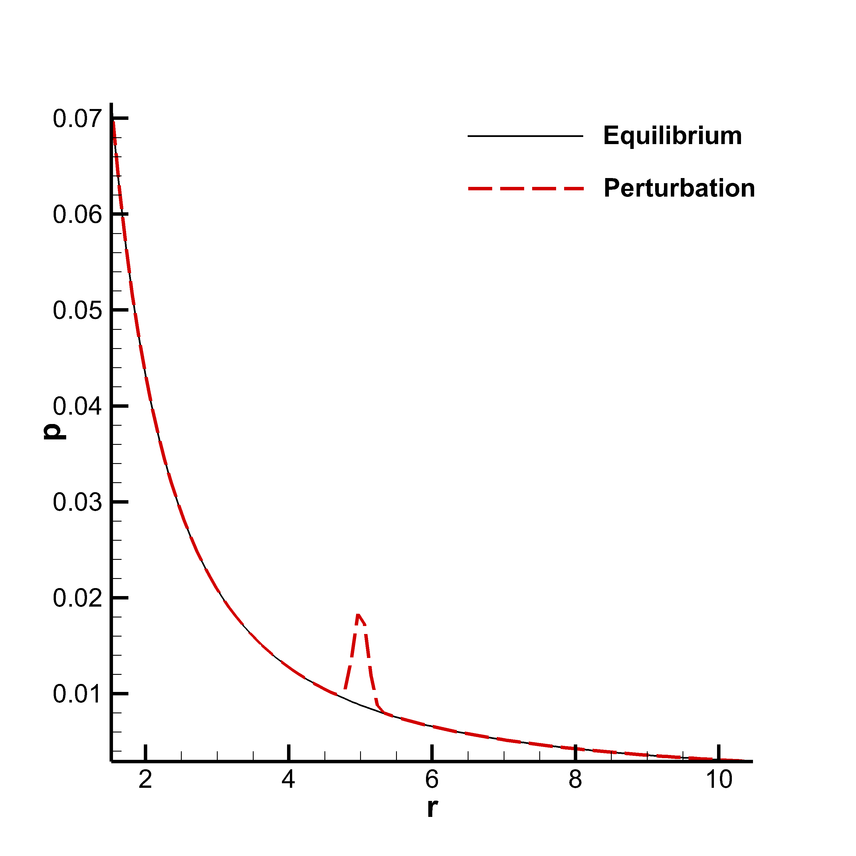
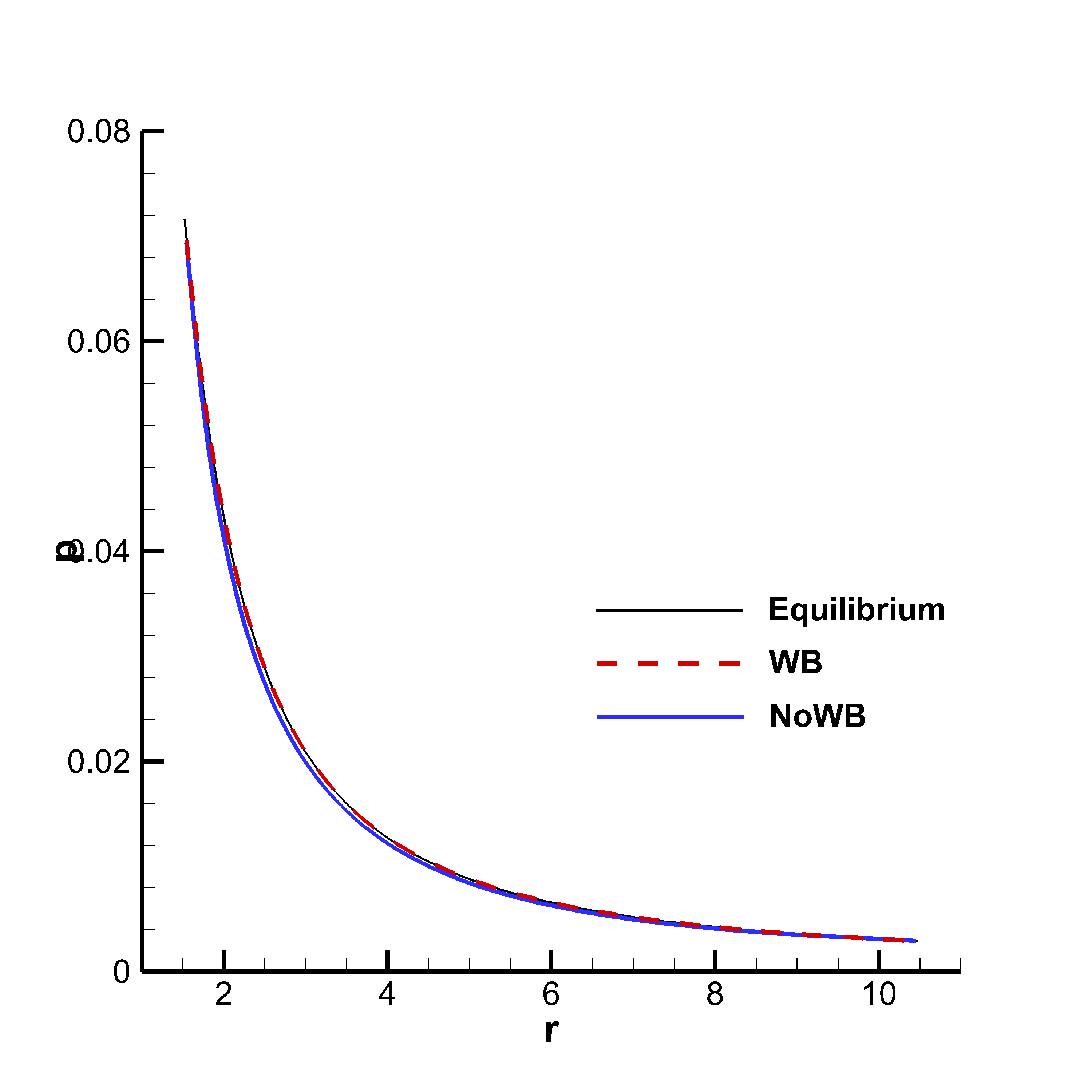
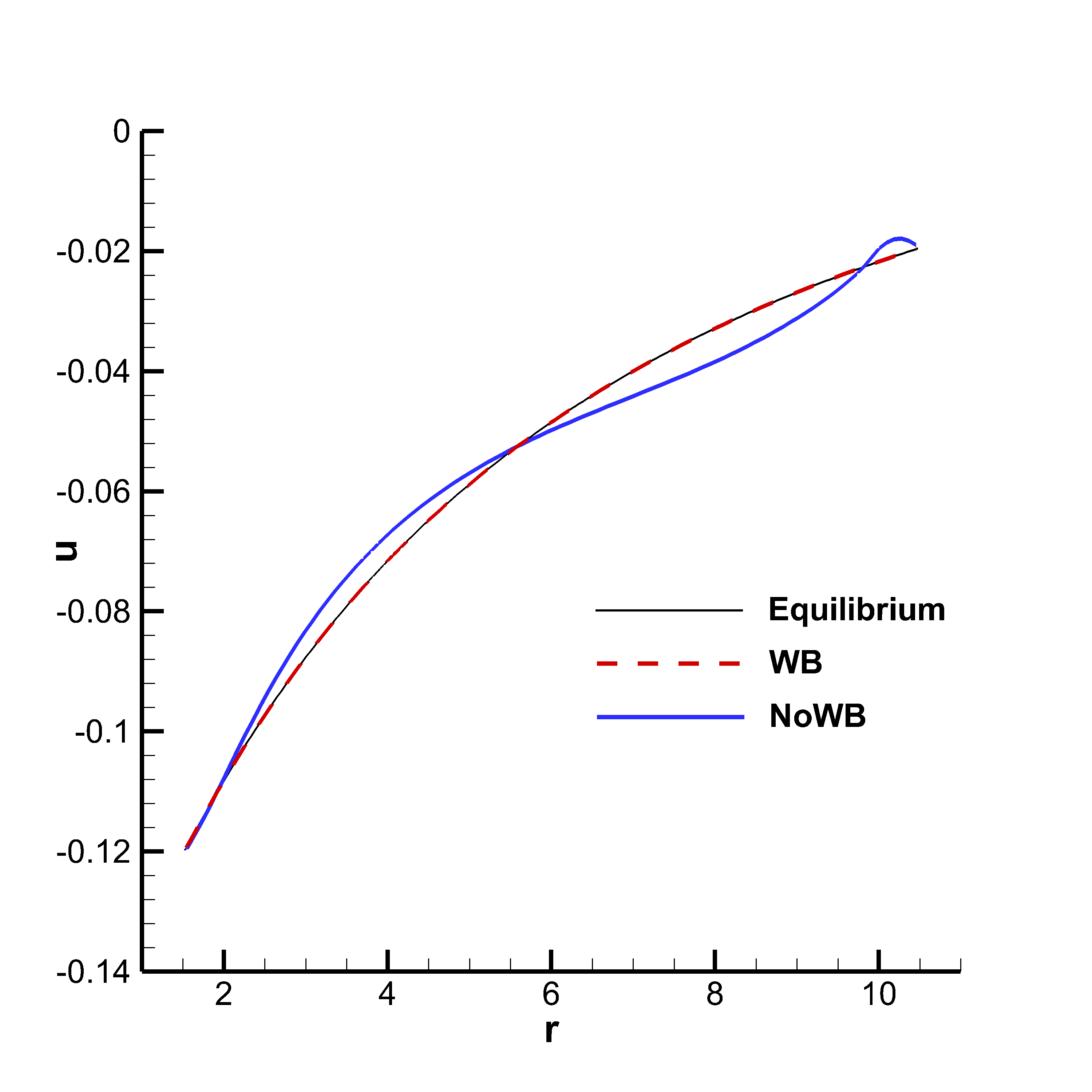
Figure 1: Michel accretion disk, equilibrium solution of GRMHD. We show the equilibrium profile (continuous black line) for pressure (left, middle) and velocity (right), and the initial perturbed pressure condition (red dashed line, left). Then, in the middle and right panels we report the numerical results obtained at time $t_{f}=10^{5}$ with the well balanced scheme (dashed red lines) and the not well balanced scheme (continuous blue lines). We remark that the initial bump is expected to split into two waves traveling out of the domain so that after a long simulation time the equilibrium profile should be recovered: this is the case with the WB scheme while the not WB scheme destroys the equilibrium profile (note in particular the completely unstable velocity profile, right panel).

We choose the second test case in order to show numerically that the WB property of the scheme, which radically improves its resolution near the equilibria, does not affect negatively any capability of the underlying second order scheme when performing simulations far away from the chosen equilibrium. Thus, while choosing as equilibrium the Michel solution over the KS coordinates described in the previous Section 4.1, we use our schemes to solve the following Riemann problem [57]

(39) $$(\rho,\mathbf{u},p,\mathbf{B})=\begin{cases}(0.125,\mathbf{0},0.1,mathbf{0})\quad\text{ if }r\leq 4\\ (1,\mathbf{0},1,mathbf{0})\quad\text{ if }r>4\end{cases}$$

over a flat Minkowski space–time, that is $\alpha=1$, $\beta^{i}=(0,0,0)$ and $\gamma_{ij}=\mathbf{I}$, on a spatial $1$D domain $\Omega$ with $x_{1}\in[2,6]$. Note that, even if the initial condition completely differs both for matter and metric from the chosen equilibrium, the WB scheme is able to return the same results of the not WB scheme, see Figure 2. Indeed far from the equilibrium the two schemes are both nominally second order accurate shock capturing TVD schemes and are expected to return equally accurate results.

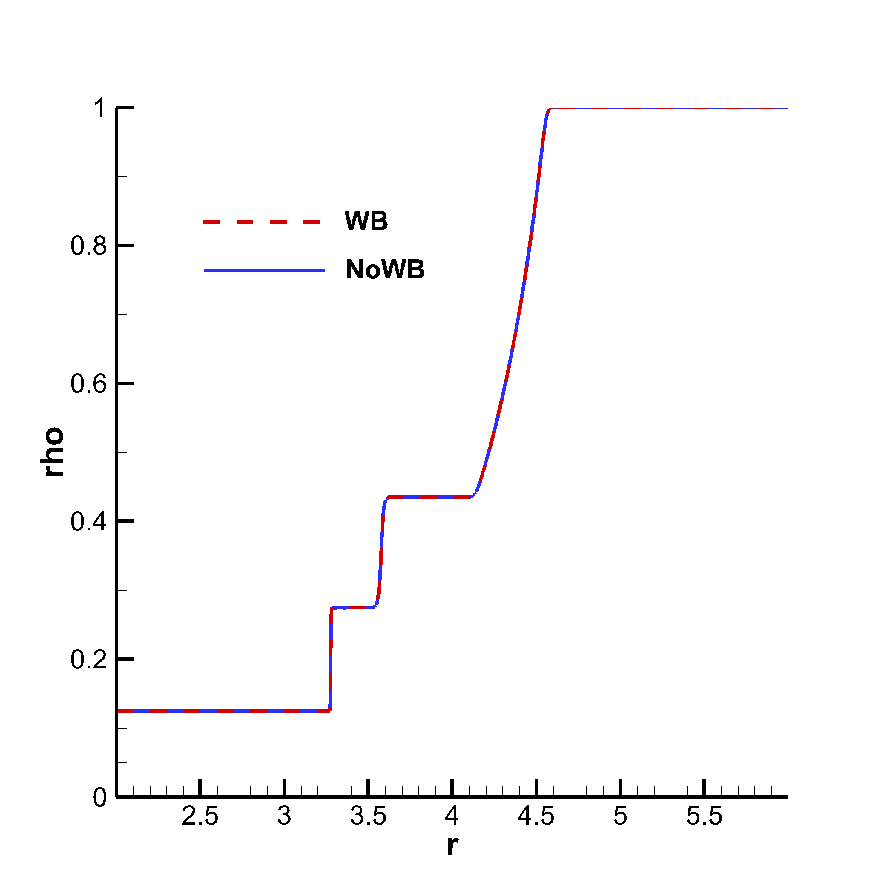
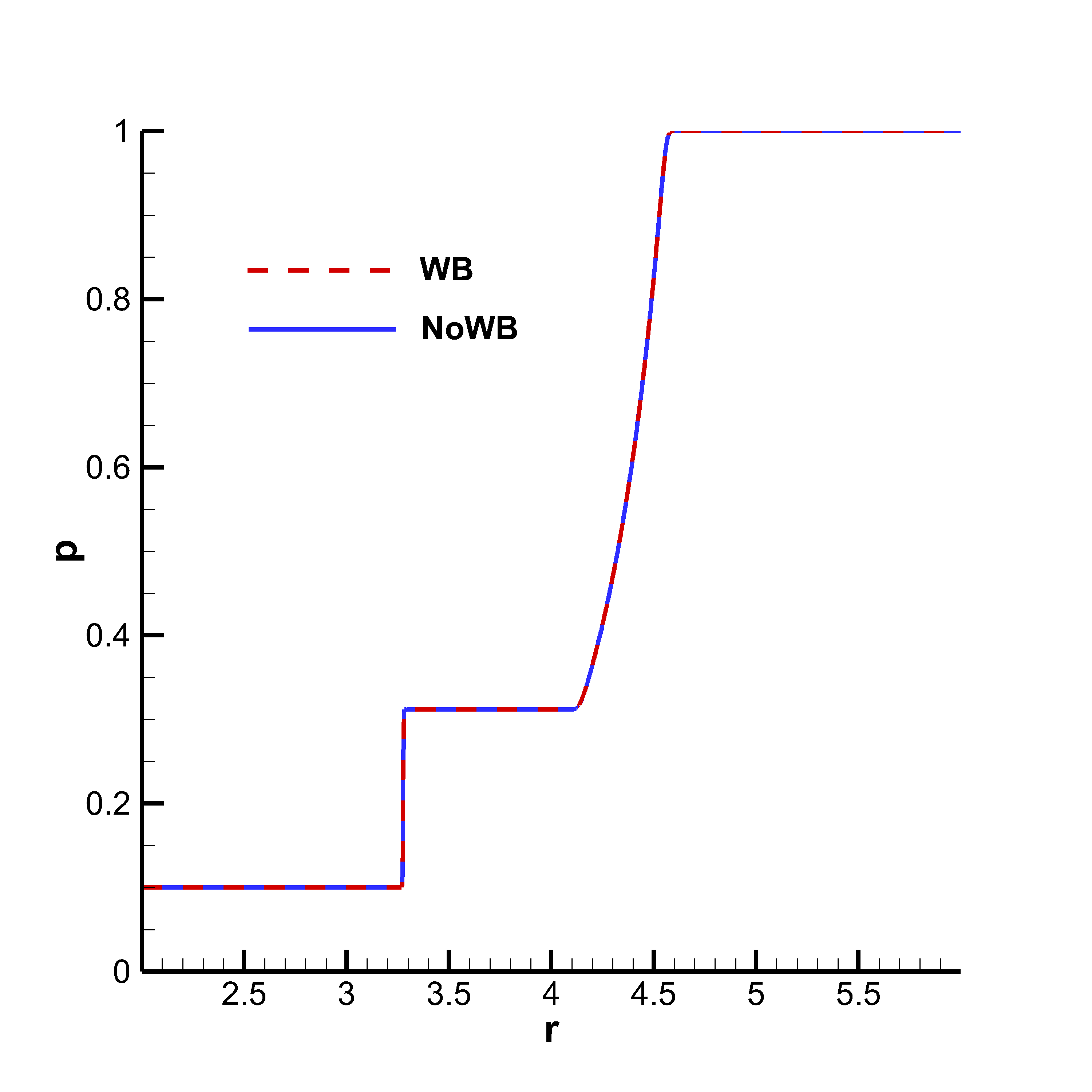
Figure 2: GRMHD Riemann problem. We show the numerical results for the density (left) and the pressure (right) obtained with a standard not WB scheme (blue) which coincide with those obtained with the new WB scheme (red) although the latter is set to maintain the Michel equilibrium.

4.3 TOV Neutron star

The next phenomenon that we want to investigate is the long time evolution of a stable Tolman-Oppenheimer-Volkoff (TOV) neutron star and the effects of small perturbations of metric and matter variables on the entire system. For the details on the derivation of the radially symmetric TOV solution, we refer to [94, 78, 98, 36, 34].

In the following, we will consider three different situations, namely the matter evolution on a fixed space–time metric through the GRMHD model (Cowling approximation), the space–time metric evolution in the anti-Cowling approximation through the FO-CCZ4 model, and the fully coupled evolution of metric and matter through the combined FO-CCZ4+GRMHD model. In the three cases we run the test problem on a $1$D domain $\Omega$ with $r\in[0.5,14]$, $\theta=\pi/2$, $\phi=0$ discretized with $N=1000$ intervals.

To impose the boundary conditions we proceed as follows. First, we use one ghost cell at each boundary set on the equilibrium value $\mathbf{Q}^{E}$. Next, we define a left and a right sponge layer $\mathcal{S_{L,R}}$ (see also [18]) so that

(40) $$x\in\mathcal{S_{L,R}}\quad\text{ if }\ |x-x_{L,R}|<s_{\mathcal{L,R}}$$

on which the numerical solution is redefined as

(41) $$\tilde{\mathbf{q}}=(1-\varepsilon_{L,R})\mathbf{q}_{h}+\varepsilon_{L,R}\mathbf{Q}^{E}.$$

These conditions are employed to impose an absorbing boundary condition which reduces the reflection of waves, and allows in particular the numerical errors traveling through the cleaning variables (as $\theta$ in the FO-CCZ4 model) to exit the domain.

To check the validity of the obtained numerical results we will monitor i) the profile of the solution, ii) the oscillation of the mass density at the center of the star, and iii) the temporal evolution of the Hamiltonian and momentum constraints, which are nonlinear elliptic involutions (hence not containing time derivatives) that should be satisfied everywhere

(42) $$\mathcal{H}=R_{ij}g^{ij}-K_{ij}K^{ij}+K^{2}-16\pi\tau=0,$$

$$\mathcal{M}_{i}=\gamma^{jl}\left(\partial_{l}K_{ij}-\partial_{i}K_{jl}-\Gamma^{m}_{\,j,l}K_{mi}+\Gamma^{m}_{\,ji}K_{ml}\right)-8\pi S_{i}=0.$$

At this point, we would like to remark that the TOV equilibrium solution is not available in the form of an analytical expression, but just as the numerical solution of a system of four ODEs (see [34] for example). Because of that, already the initial equilibrium condition does not satisfy exactly (42). Our aim will be thus preserving constantly the initial values of $\mathcal{H}$ and $\mathcal{M}_{i}$.

Finally, we emphasize that when the imposed initial conditions coincide exactly with the TOV equilibrium, the WB scheme is able to preserve it indefinitely without the introduction of any numerical errors and to perfectly maintain constants the values of the constraints. This well balanced property of our algorithm is further numerically verified in Section 4.3.1.

4.3.1 Numerical proof of the well balanced property of our algorithm

First of all, in order to present a numerical proof of the well balanced capabilities of the proposed second order well balanced scheme we have set up the following test.

Usually one claims that this property is verified when an equilibrium initial condition is preserved with machine accuracy for very long computational times. For our well balanced scheme this is trivially verified for any smooth equilibrium initial conditions $\mathbf{Q}(x,0)$ taken equal to the equilibrium profile $\mathbf{Q}^{E}$ to be preserved. Since no numerical errors are introduced by the scheme, this property can be easily verified also numerically.

To make this test more challenging and convincing, we have added a small random perturbation of the order of machine accuracy to the initial equilibrium profiles and we have monitored its evolution working in single, double and quadruple precision. We have applied this approach for all the equilibrium profiles presented in this paper. In particular, we have modified the density and the pressure when employing the GRMHD equations, and the trace of the extrinsic curvature $K$ when using the FO-CCZ4 system or the fully coupled approach, with random perturbations of the order of the corresponding machine precision used for the simulations. In Table 1 we have reported the numerical errors with respect to the equilibrium profiles for several variables of interest at short and long simulation times. In all the cases the numerical errors remain of the order of machine precision.

Table 1: Numerical proof of the well balanced property of the new well balanced finite volume scheme presented in this paper, as described in Section 4.3.1.

Precision	Single				Double				Quadruple
Time	$\Delta t$	$1$	$100$	$1000$	$\Delta t$	$1$	$100$	$1000$	$\Delta t$	$1$	$100$	$1000$
Michel
$\rho$	​1E-07	8E-08	7E-08	9E-08​	​2E-14	2E-14	4E-14	4E-14​	​1E-28	1E-28	5E-29	1E-31​
$p$	​2E-07	2E-07	2E-07	2E-07​	​1E-14	1E-14	1E-14	1E-14​	​1E-28	2E-28	1E-29	1E-32​
TOV GRMHD
$\rho$	​2E-07	3E-06	1E-05	1E-05​	​2E-14	7E-13	3E-12	2E-12​	​2E-28	7E-27	3E-26	2E-26​
$p$	​2E-07	2E-07	5E-07	2E-07​	​2E-14	2E-14	4E-14	5E-14​	​2E-28	2E-28	4E-28	3E-28​
TOV anti-Cowling
$K$	​2E-07	2E-07	3E-07	5E-07​	​2E-14	2E-14	5E-14	7E-14​	​2E-28	2E-28	2E-28	6E-28
$\theta$	​0	5E-09	7E-09	7E-09​	​4E-19	6E-15	1E-14	4E-14​	​2E-33	4E-30	2E-28	2E-27
TOV fully coupled
$\rho$	0	1E-14	1E-07	9E-06​	0	1E-19	4E-15	5E-14​	0	2E-31	1E-29	4E-30​
$K$	​2E-07	2E-07	8E-06	9E-06​	​2E-14	2E-14	8E-15	4E-14​	​2E-28	2E-28	1E-28	9E-30​
$\theta$	​1E-11	5E-08	5E-06	9E-06​	​3E-19	2E-15	9E-15	3E-14​	​1E-32	1E-30	4E-29	7E-30​
$\gamma_{11}$	0	0	1E-05	2E-05​	​2E-18	2E-15	5E-15	3E-14​	0	1E-31	1E-29	2E-29​

4.3.2 TOV neutron star simulated with the GRMHD system in Cowling approximation

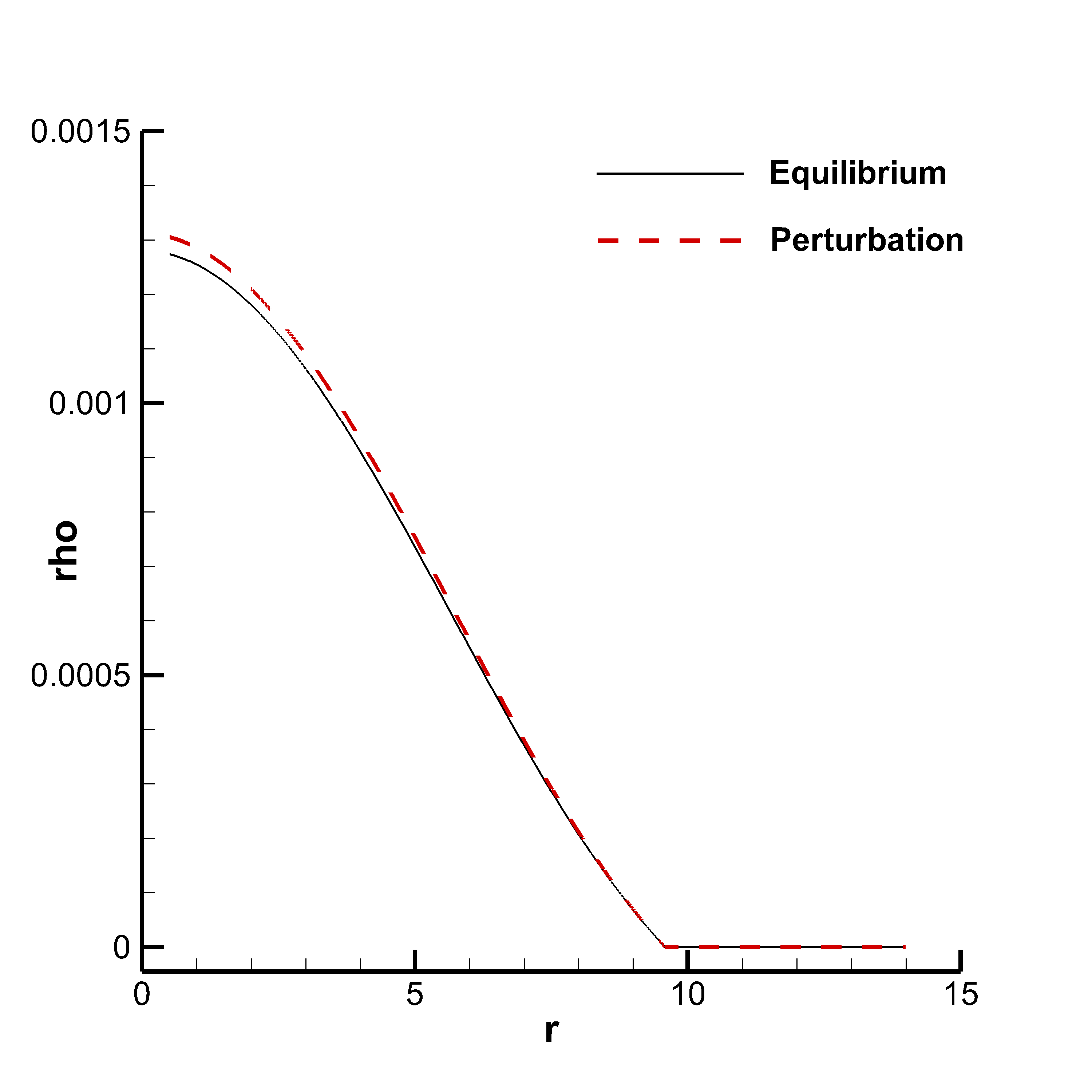
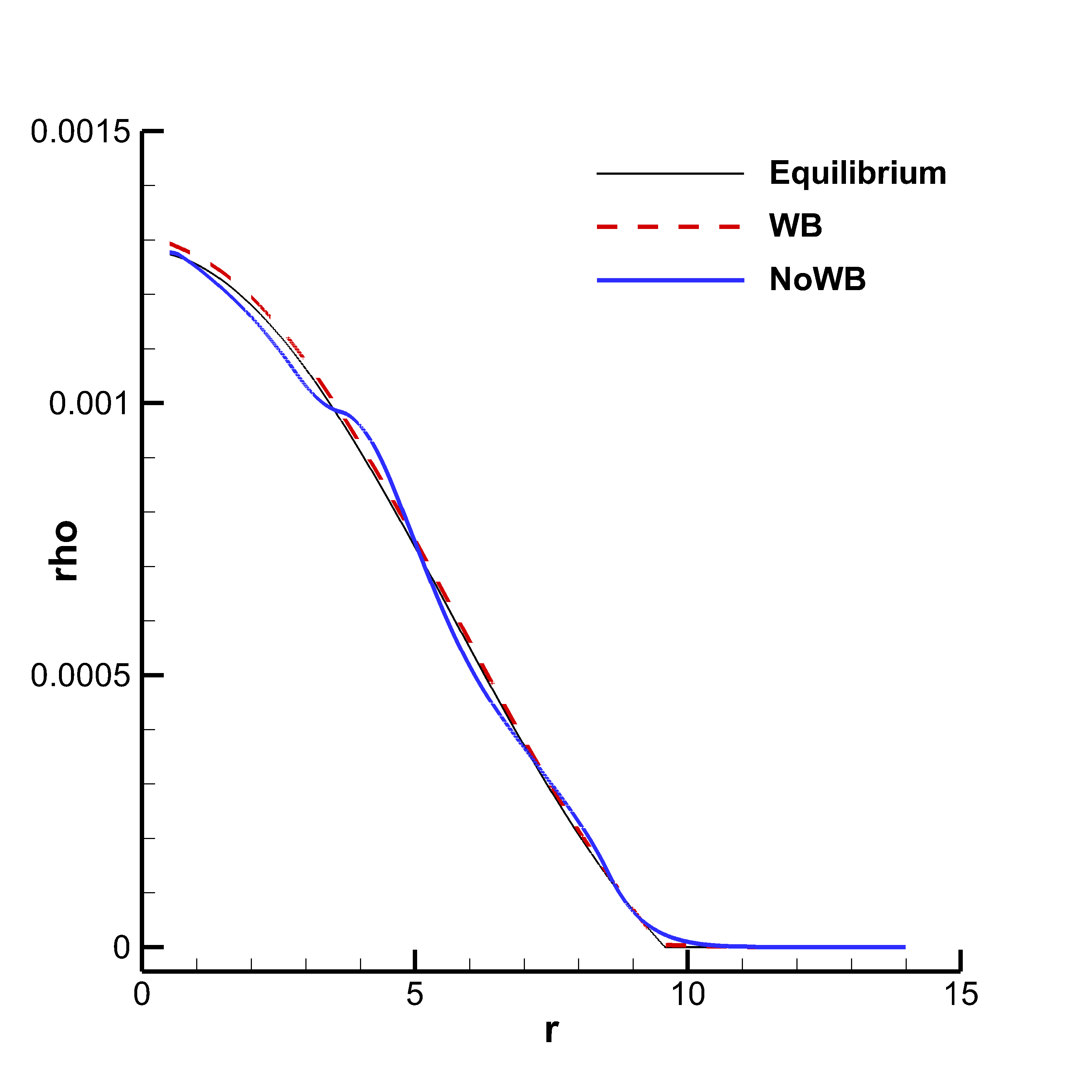
Figure 3: GRMHD TOV star simulation. We show the initial pressure perturbed profile (left) and the comparison between the equilibrium profile and the numerical results obtained with the new WB and the not WB schemes at the final time $t_{f}=10000$ (right). Note that only the WB algorithm is able to preserve the shape of the equilibrium aver long computational times.

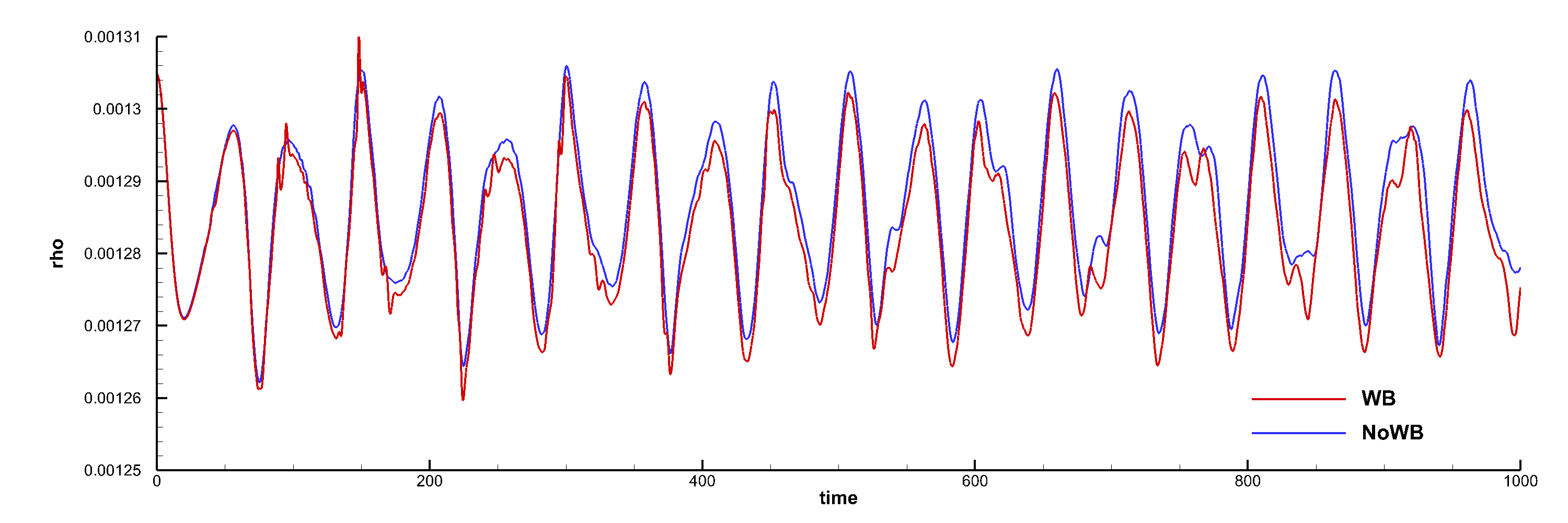
Figure 4: GRMHD TOV star simulation. We show the oscillating density of the TOV star at an inner point with $r=0.5$ over $t\in[0,1000]$ obtained with the new WB and the not WB second order schemes.

Using the GRMHD system we can simulate the evolution of the TOV neutron star on a fixed space–time metric. In particular, we have perturbed the initial equilibrium pressure profile as follows

(43) $$p=(1.0+0.05)p^{E}\quad\forall\ \mathbf{x}\text{ in }\Omega,$$

which results also in a density perturbation, being $\rho=(p/\kappa)^{1/\gamma}$, see the left panel of Figure 3. For what concerns the sponge layer, we have activated it only for the right boundary, i.e we choose $s_{\mathcal{L}}=0$, $s_{\mathcal{R}}=3$ and $\varepsilon_{R}=10^{-4}$. This allows to see the mass oscillations at the center of the star, see Figure 4.

The simulation has been run with the new WB scheme and with a standard second order not WB method. The obtained results at the final time $t_{f}=10000$ are presented in Figure 3 and they show that after long simulation times the WB scheme is still able to maintain the expected profile of the solution perfectly well, while the not WB scheme is strongly affected by the accumulation of numerical errors.

4.3.3 TOV neutron star simulated with FO-CCZ4 in the anti-Cowling approximation

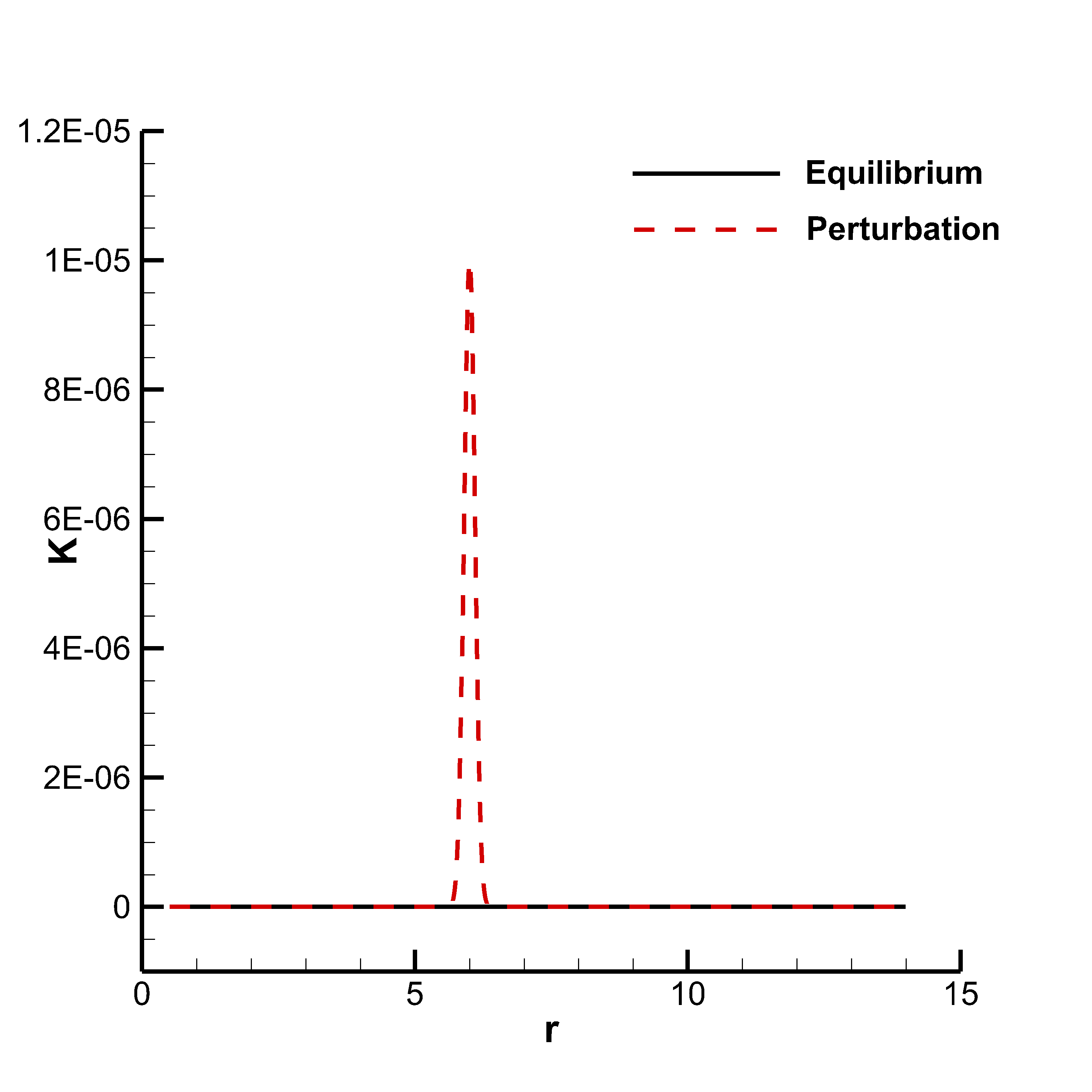
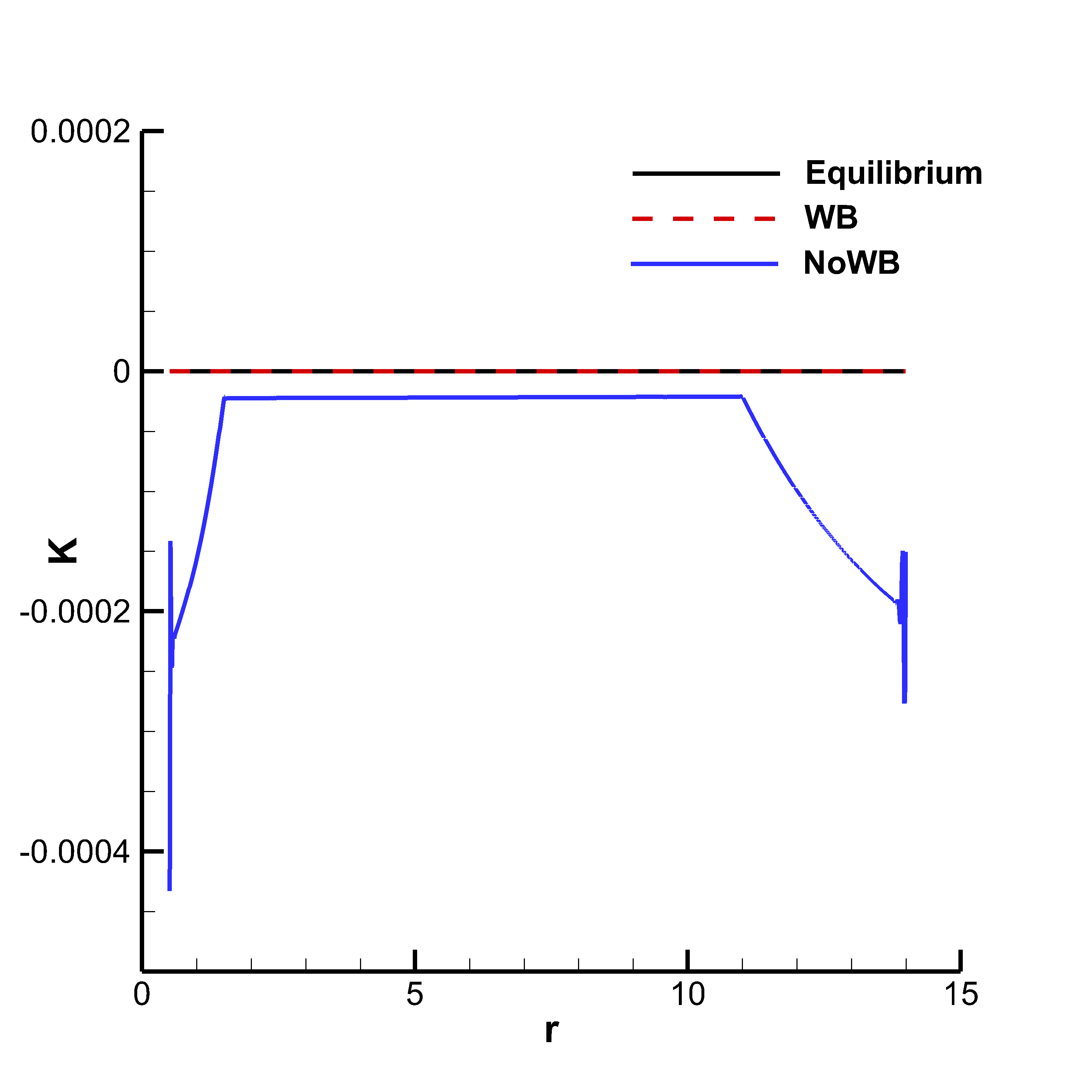
Figure 5: TOV star simulation in anti-Cowling approximation. We show the initial perturbed profile of the metric variable $K$ (left) and the comparison between the equilibrium profile and the numerical results obtained with the new WB and the not WB methods at the final time $t_{f}=1000$ (right). Note that the WB algorithm let the perturbation exit the domain and $K$ recovers its equilibrium profile while the not WB code corrupts the simulation. We underline that the error on the $K$ profile with the WB code are of the order of $10^{-9}$.

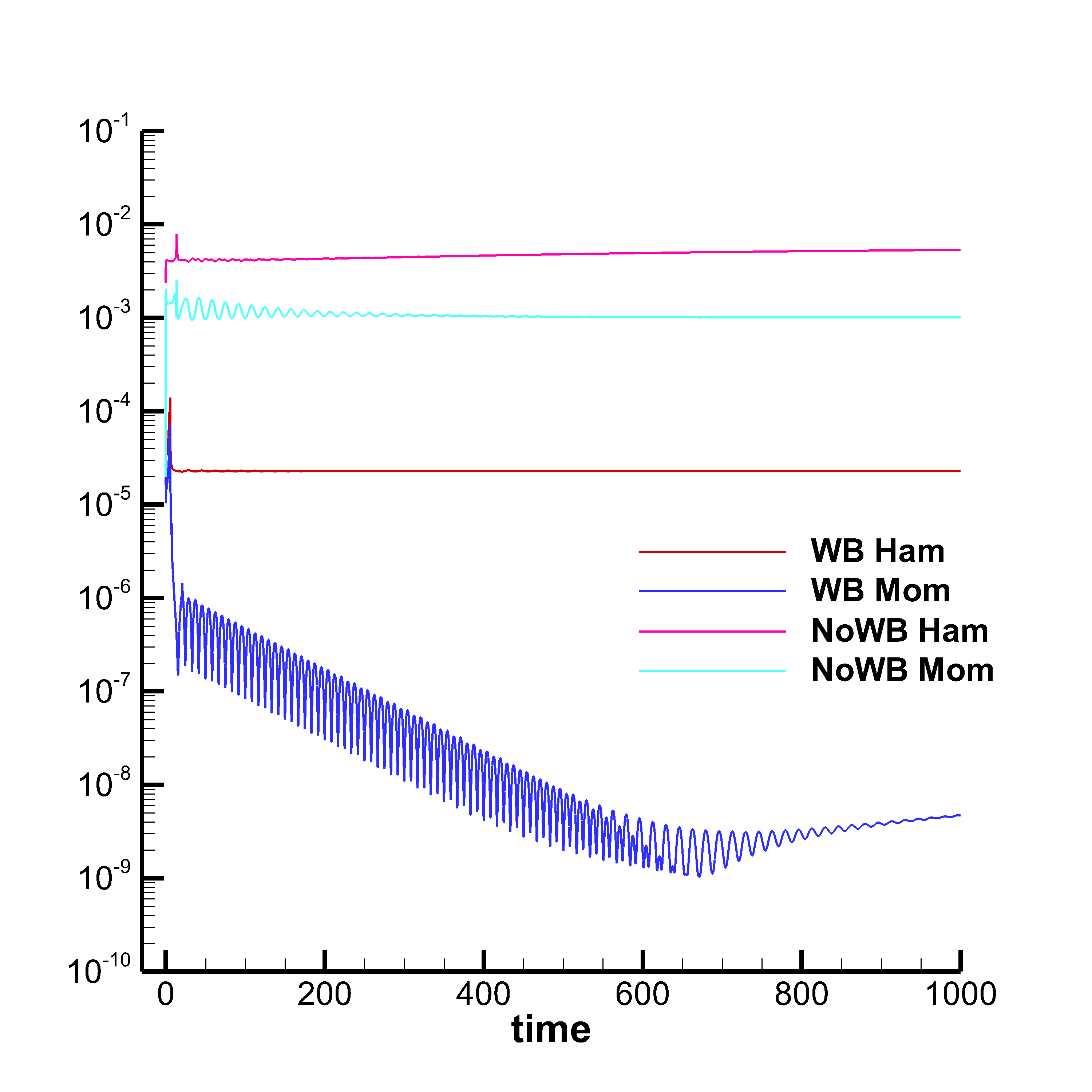
Figure 6: Hamiltonian (Ham) and momentum (Mom) constraints for the TOV star simulation in anti-Cowling approximation over the time $t\in[0,1000]$. Note i) the initial pick due to the fact that the initial perturbed profile of $K$ does not satisfy the equations, ii) the more closer to machine precision values obtained with the WB schemes for both the constraints, iii) the decreasing/slightly increasing behaviors of the constraints obtained with the WB/not WB codes.

Next, we consider the evolution of the space–time metric in the anti-Cowling approximation, i.e. we assume the matter quantities to be stationary in time and externally given by the Tolman-Oppenheimer-Volkoff (TOV) solution.

As gauge conditions we employ a frozen shift condition $\partial_{t}\beta^{i}=0$ by setting $s=0$ in the FO-CCZ4 system, together with the harmonic slicing, which corresponds to the choice $g(\alpha)=1$. The cleaning speed for the cleaning of the nonlinear ADM constraints is set to $e=1.5$. The remaining constants in the FO-CCZ4 system are chosen as $\gamma=1.4$, $\kappa_{1}=\kappa_{2}=\kappa_{3}=0$, $c=0$ and $\eta=0$.

We study here the effects of an initial perturbation over the variable $K$ so that

(44) $$K(r,0)=K^{E}(r)+10^{-5}\exp\left(-0.5\frac{(r-6.0)^{2}}{0.1^{2}}\right),$$

see also the left panel of Figure 5. The bump should split into two waves which are expected to propagate until exiting the domain. This happens when using the WB scheme where indeed the equilibrium profile of $K$ is soon recovered (with an error of $10^{-9}$ at the final time $t_{f}=1000$) while with a not WB scheme the presence of numerical errors prevents the restoring of the equilibrium, see the right panel of Figure  5. For what concerns the sponge layer, we choose $s_{\mathcal{L}}=1.0$, $s_{\mathcal{R}}=3$, $\varepsilon_{L}=10^{-3}$ and $\varepsilon_{R}=10^{-4}$ to avoid the spurious reflection of waves at the boundaries.

Finally, we monitor the Hamiltonian and momentum constraints (42) over the time, refer to Figure 6. Since the initial perturbed profile of $K$ (44) does not satisfy the equations we can notice a higher peak at the beginning of the simulation. Then, once the perturbation has exited the domain, the WB scheme is able to recover constraint values closer to zero w.r.t to the not WB scheme.

4.3.4 TOV neutron star simulated with the fully coupled FO-CCZ4 $+$ GRHD model

Finally, we consider the fully coupled model that can be obtained by considering together the FO-CCZ4 model and the GRMHD model; the initial metric values and the parameters for the ADM constraints are set as in the previous test case. In what follows we study two different perturbations of the stationary TOV neutron star profile. We would like to remark that, up to our knowledge, these are the first numerical simulations ever presented with a well balanced finite volume scheme for the fully coupled Einstein-Euler system. Long time stability is achieved thanks to the use of the novel WB techniques, which are able to stabilize the simulation and avoid the accumulation of spurious numerical errors.

Perturbation of the metric variable $\mathbf{K}$

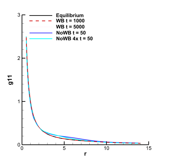
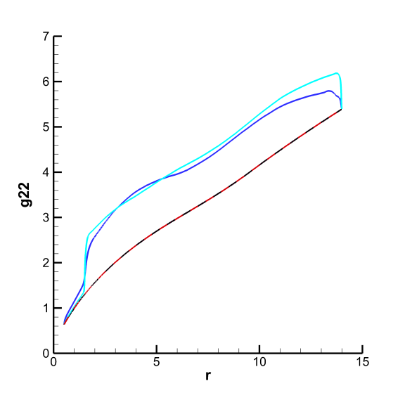
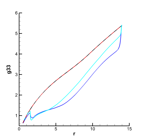
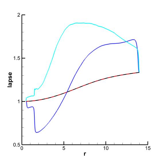
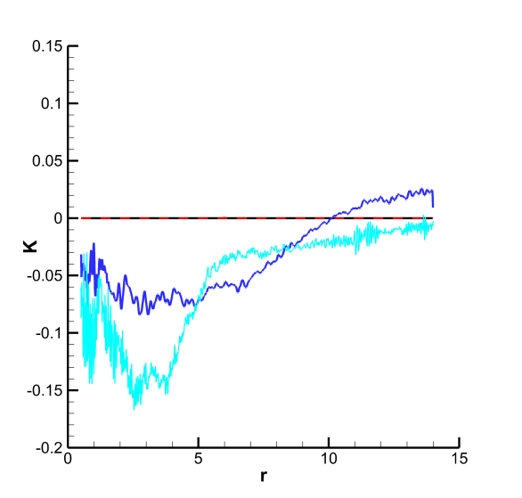
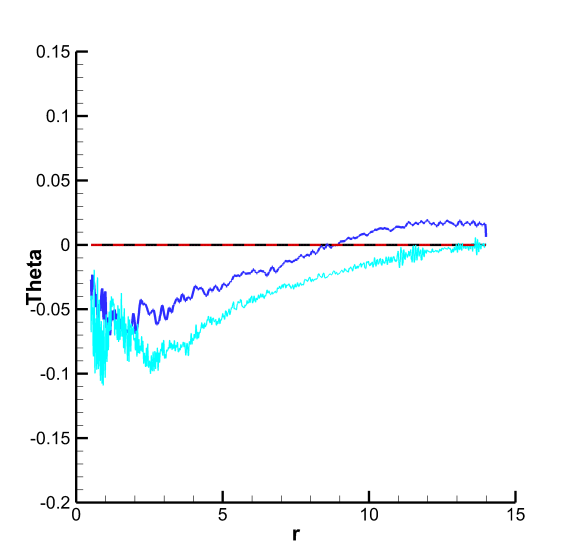
Figure 7: TOV star simulation with the CCZ4+GRHD fully coupled model corresponding to an initial perturbation over the metric variable $K$. We show: i) the expected equilibrium profile to be recovered once the perturbation has exited the domain (black line), ii) the numerical results obtained with the new WB scheme at very long times ($t=1000$ in red and $t=5000$ in pink) and iii) the completely corrupted results obtained with the not WB scheme already after a very short computational time $t=50$ (blue) even on a four time finer mesh (cyan). Plotted variables: the diagonal components of the metric $\gamma_{11}$, $\gamma_{22}$, $\gamma_{33}$, the lapse function $\lambda$, the extrinsic curvature $K$ and the cleaning variable $\theta$.

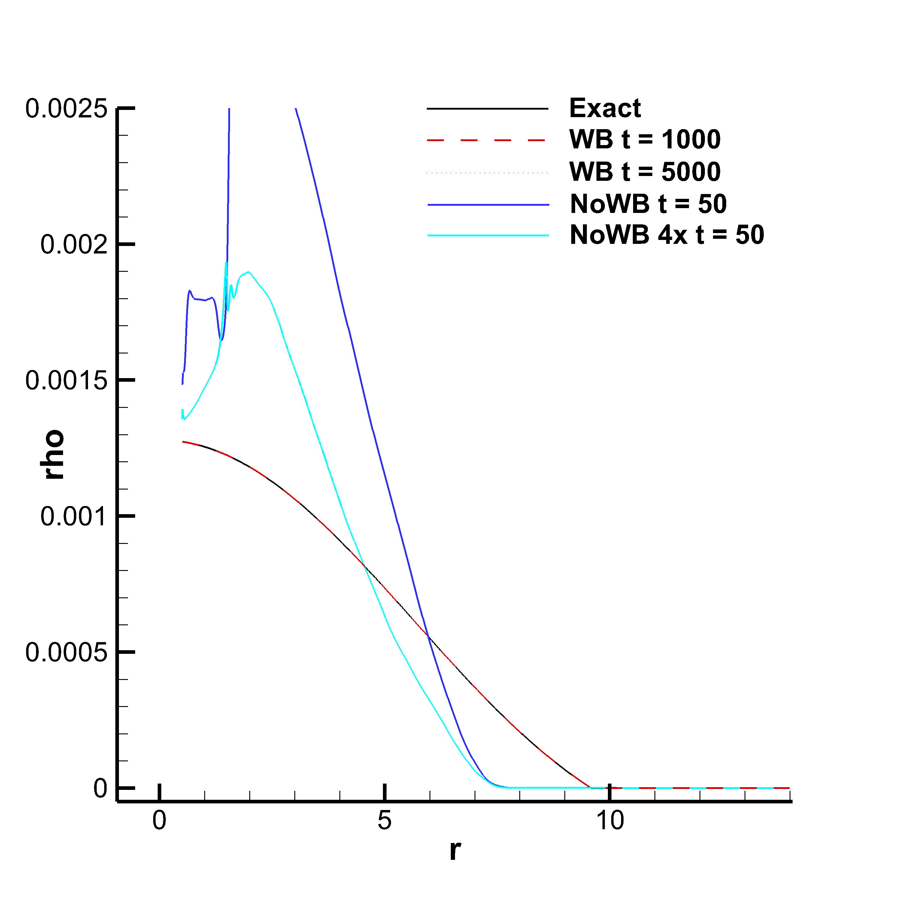
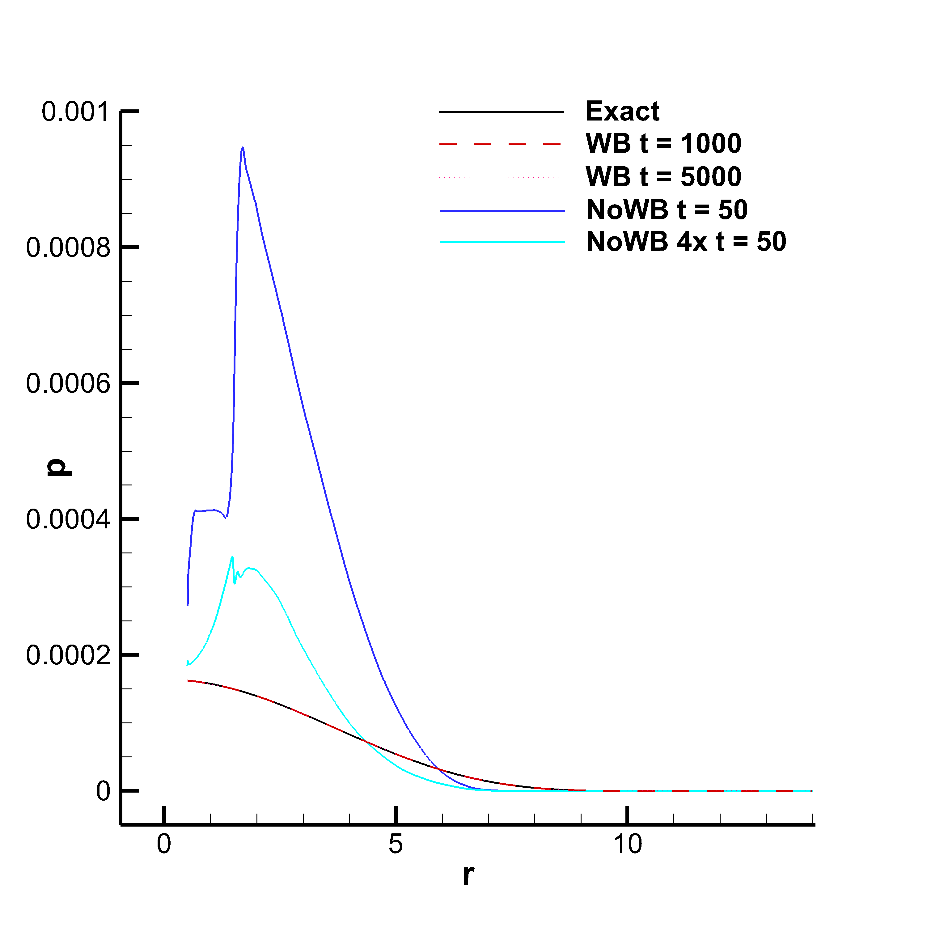
Figure 8: TOV star simulation with the CCZ4+GRHD fully coupled model corresponding to an initial perturbation over the metric variable $K$. With the same color map of the previous Figure we show here the effects of a perturbation over the metric variable $K$ on matter variables as density $\rho$ (left) and pressure $p$ (right).

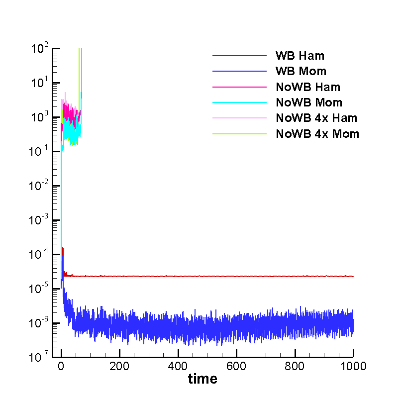
Figure 9: Hamiltonian (Ham) and momentum (Mom) constraints for the TOV star simulation with the fully coupled model over the time $t\in[0,1000]$. Note again the initial pick, the more closer to machine precision values obtained with the WB schemes already at the beginning of the simulation and in particular the fact that with the not WB code the constraints, as the entire simulation, completely blows up after a brief time while the WB code always provided trustable numerical results as evident from the perfect constraints preservation.

First, we perturb the initial value of the metric variable $K$ as in (44) and for what concerns the sponge layer, we choose $s_{\mathcal{L}}=1.0$, $s_{\mathcal{R}}=3$, $\varepsilon_{L}=10^{-3}$ and $\varepsilon_{R}=10^{-4}$.

We report in Figure 7 the profile of some metric variables and in Figure 8 the profile of the density and pressure in the matter. These results have been obtained on one hand by using the new WB scheme presented in this paper, which allows to recover and maintain the equilibrium profile even for very long simulation times of $t=1000$ or $t=5000$, and on the other hand with a standard second order scheme that, even on a four times finer mesh completely destroys the solution profile in a time of only $t=50$.

The difference in resolution and stability between the WB and not WB scheme is made evident also by the monitoring of the Hamiltonian and momentum constraints, see Figure 9: right from the beginning, the WB scheme allows a much more precise representation of the discrete solution and consequently also the errors in the involution constraints are much lower; moreover, these smaller values of $\mathcal{H}$ and $\mathcal{M}$ are almost constantly maintained in time by the WB scheme, while their values explode soon with the not WB scheme.

Perturbation of the matter variable $\mathbf{p}$

Next, we study the effect of a small pressure perturbation as the one given in (40) where, for what concerns the sponge layer, we activate it only for the right boundary, and we choose $s_{\mathcal{L}}=0$, $s_{\mathcal{R}}=3$ and $\varepsilon_{R}=10^{-4}$. Once again the constraints are more precise and better preserved with the WB scheme, see Figure 10.

For what concerns the mass oscillation at an internal point with $r=0.5$ in Figure 10 we report only the results obtained with the new WB scheme, since the not WB method, even on finer meshes, explodes after a very short time. Comparing the amplitude of this oscillation with those obtained on a fixed space–time in Figure 4 one can appreciate the different dynamic behavior obtained with a fully coupled model, where the interaction between metric and mass are taken into account, compared to the simpler GRMHD model in Cowling approximation with fixed space-time.

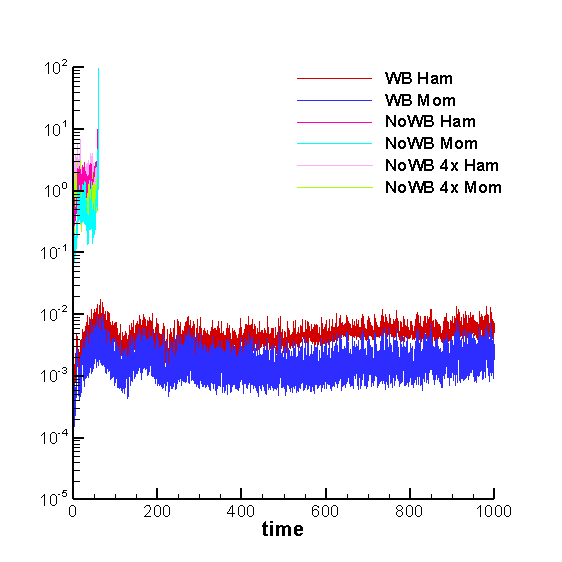
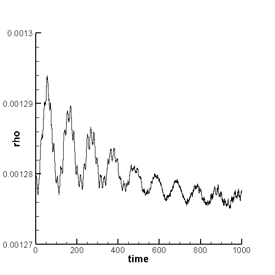
Figure 10: TOV star simulation with the CCZ4+GRHD fully coupled model corresponding to an initial perturbation over the pressure profile $p$. Left: we show the values of the Hamiltonian and momentum constraints which are close to machine precision and constantly maintained for long computational times with the WB code, while they rapidly blow up with the not WB code. Right: we plot the numerical results obtained with the new WB scheme for the density of the star at an inner point with $r=0.5$ which oscillates due to the initial pressure perturbations.

4.4 Numerical convergence studies for our well balanced algorithm

For the sake of completeness, in this last section we check the convergence rate of our new well balanced scheme by computing the experimental errors committed when solving the Michel accretion disk test case, which is an equilibrium solution of the GRMHD system known analytically (see Section 4.1), while preserving completely different equilibrium profiles, namely a i) fluid at rest immersed in a flat space-time and ii) the TOV neutron star of the previous Section 4.3. The choice of using an initial condition that completely differs from the equilibrium profiles to be preserved allows to show the second order of convergence of our well balanced method; the scheme would be instead exact when choosing to preserve an equilibrium that is equal to the initial condition of the test problem. The obtained numerical results are shown in Table 2; we would like to emphasize that the order of convergence is correctly retained even for long computational times.

Table 2: $L_{2}$ norm of the experimental errors and order of accuracy at times $t=1,10,100$ and $1000$ for the density variable $\rho$ of the Michel accretion disk test case simulated with our well balanced scheme set to preserve i) a fluid at rest over a flat space-time (top) and ii) a TOV Neutron star (bottom).

Flat ST	$t=1$		$t=10$		$t=100$		$t=1000$
$\Delta x$	$L_{2}$	$\!\!\!\!\!\!\!\!\!\!\!\mathcal{O}(L_{2})\!\!\!\!\!\!$	$L_{2}$	$\!\!\!\!\!\!\!\!\!\!\!\mathcal{O}(L_{2})\!\!\!\!\!\!$	$L_{2}$	$\!\!\!\!\!\!\!\!\!\!\!\mathcal{O}(L_{2})\!\!\!\!\!\!$	$L_{2}$	$\!\!\!\!\!\!\!\!\!\!\!\mathcal{O}(L_{2})\!\!\!\!\!\!$
9.0E-03	3.1E-06	-	4.9E-05	-	5.9E-04	-	5.0E-03	-
6.0E-03	1.4E-06	1.99	2.2E-05	1.93	2.7E-04	1.88	2.4E-03	1.79
4.5E-03	8.0E-07	1.95	1.3E-05	1.95	1.6E-04	1.91	1.4E-03	1.82
3.6E-03	5.1E-07	1.98	8.3E-06	1.96	1.0E-04	1.92	9.5E-04	1.84
3.0E-03	3.6E-07	1.97	5.8E-06	1.96	7.3E-05	1.93	6.8E-04	1.86
TOV star	$t=1$		$t=10$		$t=100$		$t=1000$
$\Delta x$	$L_{2}$	$\!\!\!\!\!\!\!\!\!\!\!\mathcal{O}(L_{2})\!\!\!\!\!\!$	$L_{2}$	$\!\!\!\!\!\!\!\!\!\!\!\mathcal{O}(L_{2})\!\!\!\!\!\!$	$L_{2}$	$\!\!\!\!\!\!\!\!\!\!\!\mathcal{O}(L_{2})\!\!\!\!\!\!$	$L_{2}$	$\!\!\!\!\!\!\!\!\!\!\!\mathcal{O}(L_{2})\!\!\!\!\!\!$
9.0E-03	2.7E-06	-	5.6E-05	-	7.2E-04	-	6.3E-03	-
6.0E-03	1.2E-06	1.99	2.6E-05	1.92	3.3E-04	1.89	3.0E-03	1.81
4.5E-03	6.9E-07	1.94	1.5E-05	1.94	1.9E-04	1.91	1.8E-03	1.84
3.6E-03	4.4E-07	1.98	9.6E-06	1.95	1.3E-04	1.92	1.2E-03	1.86
3.0E-03	3.1E-07	1.97	6.7E-06	1.96	8.8E-05	1.93	8.4E-04	1.87

5 Conclusions

With the numerical results presented here we have clearly shown the advantages that can be obtained in numerical general relativity through the use of a simple but very efficient well balancing technique. Indeed, simulations that blow up with a standard second order scheme can now be carried out in a stable manner even for very long simulation times and with accurate results, as demonstrated for example by the monitoring of the ADM constraints and the simulations carried out with the fully coupled FO-CCZ4 + GRMHD model. Moreover, we would like to underline that this preliminary work in 1D at second order of accuracy has been essential to understand model related difficulties how the setting of the cleaning and damping parameters in the FO-CCZ4 model and the boundary conditions.

Future work will concern the insertion of the presented WB techniques in already existing higher order discontinuous Galerkin schemes for modeling the GRMHD and the FO-CCZ4 systems in two or three space dimensions, as those presented in [55, 63]. In this context we will follow also the numerical approach presented in [102, 101]. Moreover, we would like to investigate the joint effect of WB and the novel GLM curl cleaning techniques introduced in [54, 43, 35]. Indeed, several systems with curl involutions have recently been investigated and attention has been devoted to the crucial role of curl involutions themselves [53] on the stability of numerical computations. With the increased level of robustness and accuracy that can be obtained at the aid of the new well balanced schemes introduced in this paper, in combination with high order DG schemes and novel curl cleaning techniques, it should therefore become possible to study also the generation and propagation of gravitational waves in the future.

Furthermore, motivated by the results obtained in [62] for the study of Keplerian disks modeled with the Euler equations with gravity and simulated with a well balanced Lagrangian scheme, we would like to apply a similar approach also for the study of general relativistic phenomena; in particular, we plan to incorporate our new well balanced techniques for GRMHD and FO-CCZ4 in modern direct Arbitrary-Lagrangian Eulerian algorithms with topology changes, as those forwarded in [90, 64, 60, 59, 44].

References

- [1] M. Alcubierre, Introduction to 3+1 numerical relativity, vol. 140, Oxford University Press, 2008.
- [2] D. Alic, C. Bona, and C. Bona-Casas, Towards a gauge-polyvalent numerical relativity code, Physical Review D, 79 (2009), p. 044026.
- [3] D. Alic, C. Bona-Casas, C. Bona, L. Rezzolla, and C. Palenzuela, Conformal and covariant formulation of the Z4 system with constraint-violation damping, Physical Review D, 85 (2012), p. 064040.
- [4] D. Alic, W. Kastaun, and L. Rezzolla, Constraint damping of the conformal and covariant formulation of the Z4 system in simulations of binary neutron stars, Physical Review D, 88 (2013), p. 064049.
- [5] M.-Á. Aloy and I. Cordero-Carrión, Minimally implicit Runge-Kutta methods for Resistive Relativistic MHD, in Journal of Physics: Conference Series, vol. 719, IOP Publishing, 2016, p. 012015.
- [6] M. A. Aloy, J. M. Ibánez, J. M. Martí, and E. Müller, GENESIS: A high-resolution code for three-dimensional relativistic hydrodynamics, The Astrophysical Journal Supplement Series, 122 (1999), p. 151.
- [7] M. Anderson, E. W. Hirschmann, L. Lehner, S. L. Liebling, P. M. Motl, D. Neilsen, C. Palenzuela, and J. E. Tohline, Magnetized neutron-star mergers and gravitational-wave signals, Physical Review Letters, 100 (2008), p. 191101.
- [8] A. Anile, Relativistic Fluids and Magneto-fluids ed AM Anile (Cambridge, UK), 1990.
- [9] A. Anile, J. Miller, and S. Motta, Formation and damping of relativistic strong shocks, The Physics of Fluids, 26 (1983), pp. 1450–1460.
- [10] P. Anninos, P. C. Fragile, and J. D. Salmonson, Cosmos++: relativistic magnetohydrodynamics on unstructured grids with local adaptive refinement, The Astrophysical Journal, 635 (2005), p. 723.
- [11] L. Antón, O. Zanotti, J. A. Miralles, J. M. Martí, J. M. Ibáñez, J. A. Font, and J. A. Pons, Numerical 3+1 general relativistic magnetohydrodynamics: a local characteristic approach, The Astrophysical Journal, 637 (2006), p. 296.
- [12] R. Arnowitt, S. Deser, and C. W. Misner, The dynamics of general relativity, Gravitation: An introduction to current research, Chap, 7 (1962), pp. 227–265.
- [13] R. Arnowitt, S. Deser, and C. W. Misner, Republication of: The dynamics of general relativity, General Relativity and Gravitation, 40 (2008), pp. 1997–2027.
- [14] L. Arpaia and M. Ricchiuto, Well balanced residual distribution for the ale spherical shallow water equations on moving adaptive meshes, Journal of Computational Physics, 405 (2020), p. 109173.
- [15] E. Audusse, F. Bouchut, M.-O. Bristeau, R. Klein, and B. t. Perthame, A fast and stable well-balanced scheme with hydrostatic reconstruction for shallow water flows, SIAM Journal on Scientific Computing, 25 (2004), pp. 2050–2065.
- [16] L. Baiotti, I. Hawke, P. J. Montero, F. Löffler, L. Rezzolla, N. Stergioulas, J. A. Font, and E. Seidel, Three-dimensional relativistic simulations of rotating neutron-star collapse to a Kerr black hole, Physical Review D, 71 (2005), p. 024035.
- [17] F. Banyuls, J. A. Font, J. M. Ibáñez, J. M. Martí, and J. A. Miralles, Numerical 3+1 general relativistic hydrodynamics: A local characteristic approach, The Astrophysical Journal, 476 (1997), p. 221.
- [18] C. Bassi, L. Bonaventura, S. Busto, and M. Dumbser, A hyperbolic reformulation of the Serre-Green-Naghdi model for general bottom topographies, Computers & Fluids, 212 (2020), p. 104716.
- [19] T. W. Baumgarte and S. L. Shapiro, Numerical integration of Einstein’s field equations, Physical Review D, 59 (1998), p. 024007.
- [20] T. W. Baumgarte and S. L. Shapiro, Numerical relativity: solving Einstein’s equations on the computer, Cambridge University Press, 2010.
- [21] J. P. Berberich, P. Chandrashekar, and C. Klingenberg, High order well-balanced finite volume methods for multi-dimensional systems of hyperbolic balance laws, Computers & Fluids, (2021), p. 104858.
- [22] A. Bermúdez, X. López, and M. E. Vázquez-Cendón, Numerical solution of non-isothermal non-adiabatic flow of real gases in pipelines, Journal of Computational Physics, 323 (2016), pp. 126–148.
- [23] A. Bermudez and M. E. Vazquez, Upwind methods for hyperbolic conservation laws with source terms, Computers & Fluids, 23 (1994), pp. 1049–1071.
- [24] S. Bernuzzi and D. Hilditch, Constraint violation in free evolution schemes: Comparing the BSSNOK formulation with a conformal decomposition of the Z4 formulation, Physical Review D, 81 (2010), p. 084003.
- [25] C. Bona, T. Ledvinka, C. Palenzuela, and M. Zácek, General-covariant evolution formalism for numerical relativity, Phys. Rev. D, 67 (2003), p. 104005.
- [26] C. Bona, T. Ledvinka, C. Palenzuela, and M. Zácek, Symmetry-breaking mechanism for the Z4 general-covariant evolution system, Phys. Rev. D, 69 (2004), p. 64036.
- [27] C. Bona, J. Masso, E. Seidel, and J. Stela, New formalism for numerical relativity, Physical Review Letters, 75 (1995), p. 600.
- [28] S. Bonazzola, E. Gourgoulhon, P. Grandclement, and J. Novak, Constrained scheme for the einstein equations based on the dirac gauge and spherical coordinates, Physical Review D, 70 (2004), p. 104007.
- [29] N. Botta, R. Klein, S. Langenberg, and S. Lützenkirchen, Well balanced finite volume methods for nearly hydrostatic flows, Journal of Computational Physics, 196 (2004), pp. 539–565.
- [30] F. Bouchut, Nonlinear stability of finite Volume Methods for hyperbolic conservation laws: And Well-Balanced schemes for sources, Springer Science & Business Media, 2004.
- [31] N. Bucciantini and L. Del Zanna, General relativistic magnetohydrodynamics in axisymmetric dynamical spacetimes: the X-ECHO code, Astronomy & Astrophysics, 528 (2011), p. A101.
- [32] N. Bucciantini and L. Del Zanna, A fully covariant mean-field dynamo closure for numerical 3+1 resistive GRMHD, Monthly Notices of the Royal Astronomical Society, 428 (2013), pp. 71–85.
- [33] M. Bugli, L. Del Zanna, and N. Bucciantini, Dynamo action in thick discs around Kerr black holes: high-order resistive GRMHD simulations, Monthly Notices of the Royal Astronomical Society: Letters, 440 (2014), pp. L41–L45.
- [34] M. Bugner, Discontinuous Galerkin methods for general relativistic hydrodynamics, PhD thesis, Friedrich-Schiller-Universität Jena, 2018.
- [35] S. Busto, M. Dumbser, C. Escalante, S. Gavrilyuk, and N. Favrie, On high order ADER discontinuous Galerkin schemes for first order hyperbolic reformulations of nonlinear dispersive systems, Journal of Scientific Computing, 87 (2021), p. 48.
- [36] S. Carroll, Spacetime and geometry. An introduction to general relativity, 2003.
- [37] M. Castro, J. Gallardo, and C. Parés, High order finite volume schemes based on reconstruction of states for solving hyperbolic systems with nonconservative products. Applications to shallow-water systems, Mathematics of computation, 75 (2006), pp. 1103–1134.
- [38] M. Castro, J. M. Gallardo, J. A. López-GarcÍa, and C. Parés, Well-balanced high order extensions of Godunov’s method for semilinear balance laws, SIAM Journal on Numerical Analysis, 46 (2008), pp. 1012–1039.
- [39] M. J. Castro, T. M. de Luna, and C. Parés, Chapter 6 - Well-balanced schemes and path-conservative numerical methods, in Handbook of Numerical Analysis, vol. 18, Elsevier, 2017, pp. 131–175.
- [40] M. J. Castro and C. Parés, Well-balanced high-order finite volume methods for systems of balance laws, Journal of Scientific Computing, 82 (2020), pp. 1–48.
- [41] P. Chandrashekar and C. Klingenberg, A second order well-balanced finite volume scheme for Euler equations with gravity, SIAM Journal on Scientific Computing, 37 (2015), pp. B382–B402.
- [42] A. Y. Chernyshenko, M. A. Olshanskii, and Y. V. Vassilevski, A hybrid finite volume–finite element method for bulk–surface coupled problems, Journal of Computational Physics, 352 (2018), pp. 516–533.
- [43] S. Chiocchetti, I. Peshkov, S. Gavrilyuk, and M. Dumbser, High order ADER schemes and GLM curl cleaning for a first order hyperbolic formulation of compressible flow with surface tension, Journal of Computational Physics, 426 (2021), p. 109898.
- [44] L. Cirrottola, M. Ricchiuto, A. Froehly, B. Re, A. Guardone, and G. Quaranta, Adaptive deformation of 3d unstructured meshes with curved body fitted boundaries with application to unsteady compressible flows, Journal of Computational Physics, 433 (2021), p. 110177.
- [45] I. Cordero-Carrión, P. Cerdá-Durán, H. Dimmelmeier, J. L. Jaramillo, J. Novak, and E. Gourgoulhon, Improved constrained scheme for the einstein equations: An approach to the uniqueness issue, Physical Review D, 79 (2009), p. 024017.
- [46] I. Cordero-Carrión, J. M. Ibanez, E. Gourgoulhon, J. L. Jaramillo, and J. Novak, Mathematical issues in a fully constrained formulation of the einstein equations, Physical Review D, 77 (2008), p. 084007.
- [47] G. Dal Maso, P. G. Lefloch, and F. Murat, Definition and weak stability of nonconservative products, Journal de mathématiques pures et appliquées, 74 (1995), pp. 483–548.
- [48] L. Del Zanna and N. Bucciantini, An efficient shock-capturing central-type scheme for multidimensional relativistic flows-I. Hydrodynamics, Astronomy & Astrophysics, 390 (2002), pp. 1177–1186.
- [49] L. Del Zanna, O. Zanotti, N. Bucciantini, and P. Londrillo, ECHO: a Eulerian conservative high-order scheme for general relativistic magnetohydrodynamics and magnetodynamics, Astronomy & Astrophysics, 473 (2007), pp. 11–30.
- [50] V. Desveaux, M. Zenk, C. Berthon, and C. Klingenberg, A well-balanced scheme to capture non-explicit steady states in the Euler equations with gravity, International Journal for Numerical Methods in Fluids, 81 (2016), pp. 104–127.
- [51] K. Dionysopoulou, D. Alic, C. Palenzuela, L. Rezzolla, and B. Giacomazzo, General-relativistic resistive magnetohydrodynamics in three dimensions: Formulation and tests, Physical Review D, 88 (2013), p. 044020.
- [52] M. D. Duez, Y. T. Liu, S. L. Shapiro, and B. C. Stephens, Relativistic magnetohydrodynamics in dynamical spacetimes: Numerical methods and tests, Physical Review D, 72 (2005), p. 024028.
- [53] M. Dumbser, S. Chiocchetti, and I. Peshkov, On numerical methods for hyperbolic pde with curl involutions, Continuum Mechanics, Applied Mathematics and Scientific Computing: Godunov’s Legacy, Springer, (2020), pp. 125–134.
- [54] M. Dumbser, F. Fambri, E. Gaburro, and A. Reinarz, On GLM curl cleaning for a first order reduction of the CCZ4 formulation of the Einstein field equations, Journal of Computational Physics, 404 (2020), p. 109088.
- [55] M. Dumbser, F. Guercilena, S. Köppel, L. Rezzolla, and O. Zanotti, Conformal and covariant Z4 formulation of the Einstein equations: Strongly hyperbolic first-order reduction and solution with discontinuous Galerkin schemes, Physical Review D, 97 (2018), p. 084053.
- [56] M. Dumbser and O. Zanotti, Very high order PNPM schemes on unstructured meshes for the resistive relativistic MHD equations, Journal of Computational Physics, 228 (2009), pp. 6991–7006.
- [57] F. Fambri, M. Dumbser, S. Köppel, L. Rezzolla, and O. Zanotti, ADER discontinuous Galerkin schemes for general-relativistic ideal magnetohydrodynamics, Monthly Notices of the Royal Astronomical Society, 477 (2018), pp. 4543–4564.
- [58] J. A. Font, Numerical hydrodynamics and magnetohydrodynamics in general relativity, Living Reviews in Relativity, 11 (2008), pp. 1–131.
- [59] E. Gaburro, A Unified Framework for the Solution of Hyperbolic PDE Systems Using High Order Direct Arbitrary-Lagrangian–Eulerian Schemes on Moving Unstructured Meshes with Topology Change, Archives of Computational Methods in Engineering, (2020).
- [60] E. Gaburro, W. Boscheri, S. Chiocchetti, C. Klingenberg, V. Springel, and M. Dumbser, High order direct Arbitrary-Lagrangian-Eulerian schemes on moving Voronoi meshes with topology changes, Journal of Computational Physics, 407 (2020), p. 109167.
- [61] E. Gaburro, M. J. Castro, and M. Dumbser, A well balanced diffuse interface method for complex nonhydrostatic free surface flows, Computers & Fluids, 175 (2018), pp. 180–198.
- [62] E. Gaburro, M. J. Castro, and M. Dumbser, Well-balanced Arbitrary-Lagrangian-Eulerian finite volume schemes on moving nonconforming meshes for the Euler equations of gas dynamics with gravity, Monthly Notices of the Royal Astronomical Society, 477 (2018), pp. 2251–2275.
- [63] E. Gaburro and M. Dumbser, A Posteriori Subcell Finite Volume Limiter for General PNPM Schemes: Applications from Gasdynamics to Relativistic Magnetohydrodynamics, Journal of Scientific Computing, 86 (2021), pp. 1–41.
- [64] E. Gaburro, M. Dumbser, and M. J. Castro, Direct Arbitrary-Lagrangian-Eulerian finite volume schemes on moving nonconforming unstructured meshes, Computers & Fluids, 159 (2017), pp. 254–275.
- [65] B. Giacomazzo and L. Rezzolla, WhiskyMHD: a new numerical code for general relativistic magnetohydrodynamics, Classical and Quantum Gravity, 24 (2007), p. S235.
- [66] L. Gosse, A well-balanced scheme using non-conservative products designed for hyperbolic systems of conservation laws with source terms, Mathematical Models and Methods in Applied Sciences, 11 (2001), pp. 339–365.
- [67] L. Grosheintz-Laval and R. Käppeli, High-order well-balanced finite volume schemes for the Euler equations with gravitation, Journal of Computational Physics, 378 (2019), pp. 324–343.
- [68] C. Gundlach and J. M. Martin-Garcia, Hyperbolicity of second order in space systems of evolution equations, Classical and Quantum Gravity, 23 (2006), p. S387.
- [69] R. Käppeli and S. Mishra, Well-balanced schemes for the Euler equations with gravitation, Journal of Computational Physics, 259 (2014), pp. 199–219.
- [70] R. Käppeli and S. Mishra, A well-balanced finite volume scheme for the euler equations with gravitation-the exact preservation of hydrostatic equilibrium with arbitrary entropy stratification, Astronomy & Astrophysics, 587 (2016), p. A94.
- [71] K. Kiuchi, Y. Sekiguchi, M. Shibata, and K. Taniguchi, Long-term general relativistic simulation of binary neutron stars collapsing to a black hole, Physical Review D, 80 (2009), p. 064037.
- [72] C. Klingenberg, G. Puppo, and M. Semplice, Arbitrary order finite volume well-balanced schemes for the Euler equations with gravity, SIAM Journal on Scientific Computing, 41 (2019), pp. A695–A721.
- [73] S. Komissarov, General relativistic magnetohydrodynamic simulations of monopole magnetospheres of black holes, Monthly Notices of the Royal Astronomical Society, 350 (2004), pp. 1431–1436.
- [74] R. J. LeVeque, Balancing source terms and flux gradients in high-resolution Godunov methods: the quasi-steady wave-propagation algorithm, Journal of computational physics, 146 (1998), pp. 346–365.
- [75] J. M. Martí and E. Müller, Grid-based methods in relativistic hydrodynamics and magnetohydrodynamics, Living reviews in computational astrophysics, 1 (2015), pp. 1–182.
- [76] F. C. Michel, Accretion of matter by condensed objects, Astrophysics and Space Science, 15 (1972), pp. 153–160.
- [77] T. Nakamura, K. Oohara, and Y. Kojima, General relativistic collapse to black holes and gravitational waves from black holes, Progress of Theoretical Physics Supplement, 90 (1987), pp. 1–218.
- [78] J. R. Oppenheimer and G. M. Volkoff, On massive neutron cores, Physical Review, 55 (1939), p. 374.
- [79] C. Palenzuela, L. Lehner, O. Reula, and L. Rezzolla, Beyond ideal MHD: towards a more realistic modelling of relativistic astrophysical plasmas, Monthly Notices of the Royal Astronomical Society, 394 (2009), pp. 1727–1740.
- [80] C. Parés, Numerical methods for nonconservative hyperbolic systems: a theoretical framework., SIAM Journal on Numerical Analysis, 44 (2006), pp. 300–321.
- [81] B. Perthame and C. Simeoni, A kinetic scheme for the Saint-Venant system with a source term, Calcolo, 38 (2001), pp. 201–231.
- [82] O. Porth, H. Olivares, Y. Mizuno, Z. Younsi, L. Rezzolla, M. Moscibrodzka, H. Falcke, and M. Kramer, The black hole accretion code, Computational Astrophysics and Cosmology, 4 (2017), pp. 1–42.
- [83] D. Radice and L. Rezzolla, THC: a new high-order finite-difference high-resolution shock-capturing code for special-relativistic hydrodynamics, Astronomy & Astrophysics, 547 (2012), p. A26.
- [84] D. Radice, L. Rezzolla, and F. Galeazzi, Beyond second-order convergence in simulations of binary neutron stars in full general relativity, Monthly Notices of the Royal Astronomical Society: Letters, 437 (2013), pp. L46–L50.
- [85] T. C. Rebollo, A. D. Delgado, and E. D. F. Nieto, A family of stable numerical solvers for the shallow water equations with source terms, Computer methods in applied mechanics and engineering, 192 (2003), pp. 203–225.
- [86] L. Rezzolla and O. Zanotti, Relativistic hydrodynamics, Oxford University Press, 2013.
- [87] G. Russo and A. Anile, Stability properties of relativistic shock waves: basic results, The Physics of fluids, 30 (1987), pp. 2406–2413.
- [88] K. Schaal, A. Bauer, P. Chandrashekar, R. Pakmor, C. Klingenberg, and V. Springel, Astrophysical hydrodynamics with a high-order discontinuous Galerkin scheme and adaptive mesh refinement, Monthly Notices of the Royal Astronomical Society, 453 (2015), pp. 4278–4300.
- [89] M. Shibata and T. Nakamura, Evolution of three-dimensional gravitational waves: Harmonic slicing case, Physical Review D, 52 (1995), p. 5428.
- [90] V. Springel, E pur si muove: Galilean-invariant cosmological hydrodynamical simulations on a moving mesh, Monthly Notices of the Royal Astronomical Society, 401 (2010), pp. 791–851.
- [91] R. Takahashi and M. Umemura, General relativistic radiative transfer code in rotating black hole space–time: ARTIST, Monthly Notices of the Royal Astronomical Society, 464 (2016), pp. 4567–4585.
- [92] H. Tang, T. Tang, and K. Xu, A gas-kinetic scheme for shallow-water equations with source terms, Zeitschrift für angewandte Mathematik und Physik ZAMP, 55 (2004), pp. 365–382.
- [93] A. Thomann, M. Zenk, and C. Klingenberg, A second-order positivity-preserving well-balanced finite volume scheme for Euler equations with gravity for arbitrary hydrostatic equilibria, International Journal for Numerical Methods in Fluids, 89 (2019), pp. 465–482.
- [94] R. C. Tolman, Static solutions of Einstein’s field equations for spheres of fluid, Physical Review, 55 (1939), p. 364.
- [95] E. F. Toro, Riemann Solvers and Numerical Methods for Fluid Dynamics, Springer, second ed., 1999.
- [96] B. Van Leer, Towards the ultimate conservative difference scheme. II. Monotonicity and conservation combined in a second-order scheme, Journal of computational physics, 14 (1974), pp. 361–370.
- [97] B. Van Leer, Towards the ultimate conservative difference scheme. V. A second-order sequel to Godunov’s method, Journal of computational Physics, 32 (1979), pp. 101–136.
- [98] R. M. Wald, General relativity(Book), Chicago, University of Chicago Press, 1984, 504 p, (1984).
- [99] C. J. White, J. M. Stone, and C. F. Gammie, An extension of the Athena++ code framework for GRMHD based on advanced Riemann solvers and staggered-mesh constrained transport, The Astrophysical Journal Supplement Series, 225 (2016), p. 22.
- [100] J. R. Wilson, Some magnetic effects in stellar collapse and accretion, tech. report, California Univ., Livermore (USA). Lawrence Livermore Lab., 1975.
- [101] Y. Xing, Exactly well-balanced discontinuous Galerkin methods for the shallow water equations with moving water equilibrium, Journal of Computational Physics, 257 (2014), pp. 536–553.
- [102] Y. Xing and C.-W. Shu, High order well-balanced finite volume WENO schemes and discontinuous Galerkin methods for a class of hyperbolic systems with source terms, Journal of Computational Physics, 214 (2006), pp. 567–598.