Few-shot Unsupervised Domain Adaptation with Image-to-class Sparse Similarity Encoding

Abstract.

This paper investigates a valuable setting called few-shot unsupervised domain adaptation (FS-UDA), which has not been sufficiently studied in the literature. In this setting, the source domain data are labelled, but with few-shot per category, while the target domain data are unlabelled. To address the FS-UDA setting, we develop a general UDA model to solve the following two key issues: the few-shot labeled data per category and the domain adaptation between support and query sets. Our model is general in that once trained it will be able to be applied to various FS-UDA tasks from the same source and target domains. Inspired by the recent local descriptor based few-shot learning (FSL), our general UDA model is fully built upon local descriptors (LDs) for image classification and domain adaptation. By proposing a novel concept called similarity patterns (SPs), our model not only effectively considers the spatial relationship of LDs that was ignored in previous FSL methods, but also makes the learned image similarity better serve the required domain alignment. Specifically, we propose a novel IMage-to-class sparse Similarity Encoding (IMSE) method. It learns SPs to extract the local discriminative information for classification and meanwhile aligns the covariance matrix of the SPs for domain adaptation. Also, domain adversarial training and multi-scale local feature matching are performed upon LDs. Extensive experiments conducted on a multi-domain benchmark dataset DomainNet demonstrates the state-of-the-art performance of our IMSE for the novel setting of FS-UDA. In addition, for FSL, our IMSE can also show better performance than most of recent FSL methods on miniImageNet.

1. Introduction

Unsupervised domain adaptation (UDA) leverages sufficient labeled data in a source domain to classify unlabeled data in a target domain (Tzeng et al., 2017; Saito et al., 2018; Tzeng et al., 2014). Since the source domain usually has a different distribution from the target domain, most existing UDA methods (Hu et al., 2020; Saito et al., 2018; Cao et al., 2018) have been developed to reduce the domain gap between both domains. However, in real cases, when the source domain suffers from high annotation cost or the limited access to labeled data, the labeled data in source domain could become seriously insufficient. This makes the learning of a UDA model more challenging. On the other hand, existing UDA methods usually train a specific UDA model for a certain task with given categories, and thus cannot be efficiently updated to classify unseen categories in a new task. Recently, the need of handling few-shot labeled source domain data and having a general UDA model that can quickly adapt to many new tasks has been seen in a number of real applications.

For example, in the online shopping, sellers generally show a few photos professionally taken by photographers for each product (as source domain), while buyers usually search for their expected products by using the photos directly taken by their cellphones (as target domain). Since different buyers usually submit the images of products with different categories and types, the online shopping system needs to have a general domain adaptation model to classify the types of these products, whatever their categories are. Also, we take another example. The database of ID card usually only stores one photo for each person and these ID photos are captured in photo studios with well controlled in-door lighting conditions (as source domain). However, in many cases, an intelligence system needs to identity these persons by matching with their facial pictures captured by smartphones, ATM cameras, or even surveillance cameras in open environments (as target domain).

This situation motivates us to focus on a valuable but insufficiently studied setting, few-shot unsupervised domain adaptation (FS-UDA). A FS-UDA task includes a support set from the source domain and a query set from the target domain. The support set contains few labeled source domain samples per category, while the query set contains unlabeled target domain samples to be classified. The goal is to train a general model to handle various FS-UDA tasks from the same source and target domains. These tasks realize classification of different category sets in the target domain.

Our solution to this FS-UDA setting is inspired by few-shot learning (FSL). Recent metric based FSL methods (Vinyals et al., 2016; Snell et al., 2017; Li et al., 2019a; Zhang et al., 2020) usually learn a feature embedding model for image-to-class measurement, and meanwhile perform episodic training to make the model generalized to new tasks without any retraining or fine-tuning process. Considering the domain gap between the support and query sets in the proposed setting of FS-UDA, we tactically perform episodic training on an auxiliary dataset that contains the data from both domains, aiming to learn a general and domain-shared feature embedding model. For each episode, a few samples from both domains are randomly sampled from the auxiliary dataset to train the model.

Also, for efficient image-to-class measurement, several recent methods (Li et al., 2019a; Zhang et al., 2020; Li et al., 2020) leveraged local descriptors (LDs) of images, because they can better provide discriminative and transferable information across categories, which can be important cues for image classification in FSL (Zhang et al., 2020). These methods first measured the similarities (or distances) between the LDs of a query image and a support class by using cosine (Li et al., 2019a), KL divergence (Li et al., 2020) or EMD distance (Zhang et al., 2020), and then combined these similarities to produce a single image-to-class similarity score for classification. We believe that for two LDs that are spatially adjacent and therefore highly likely similar to each other, their similarity values to other LDs should be close and change in a smooth manner. However, the above FSL methods did not effectively take the spatial relationship of the LDs into account, and could result in noisy or non-smooth similarities w.r.t. the spatial dimension (e.g. caused by outliers, occlusion or background clutter in images). Moreover, considering the key role of image-to-class similarities for classification, we leverage them to align the source and target domains. Nevertheless, merely having a single similarity score as produced in the above methods cannot effectively serve the domain alignment required in our FS-UDA.

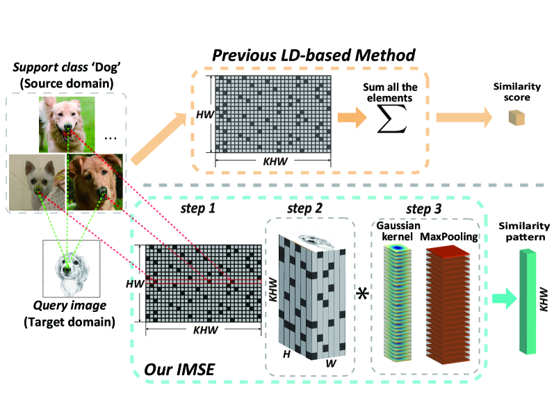
Figure 1. Illustration of encoding a similarity pattern in our IMSE, compared with a single similarity score produced in previous LD-based FSL methods (e.g. DN4 (Li et al., 2019a), ADM (Li et al., 2020), DeepEMD (Zhang et al., 2020)). For a similarity pattern, we first calculate the similarity matrix between LDs of a query image to a support class, and only maintain the top-$k$ similarities for each row. Then, the similarity matrix is reshaped into a 3D map whose spatial sizes are the same as those of the query image. Afterwards, we conduct a Gaussian filter and max-pooling operation to smooth and aggregate the similarity of the spatially-adjacent LDs of the query image, and thus generate an image-to-class SP finally. Here, $H$ and $W$ denote the height and weight of the feature map, and $K$ denotes the number of images per support class.

Therefore, instead of computing a single similarity score, we design a novel image-to-class similarity pattern (SP) vector that contains the similarities of a query image to all LDs of a support class. We design a Gaussian filter and a max-pooling module on the spatial dimension of query images, which can smooth the similarities of spatially-adjacent LDs and extract the prominent similarity. Thus, SP provides a fine-grained and patterned measurement for classification. Also, the SPs of query images can be leveraged as their features for domain alignment. To this end, we align the covariance matrix of the SPs between domains, because covariance matrix can naturally capture the underlying data distribution (Li et al., 2019b). For further domain alignment, we also perform domain adversarial training and multi-scale matching on LDs. In doing so, we propose a novel method, IMage-to-class sparse Similarity Encoding (IMSE), which learns image-to-class similarity patterns to realize effective classification and domain adaptation. Figure 1 illustrates the encoding process of SPs. Our contributions can be summarized as:

1. A novel method for the new setting of FS-UDA. We propose a novel method IMSE for a valuable but insufficiently studied setting FS-UDA, which learns a domain-shared feature embedding model and adapts this general model to handle various new tasks.

2. A novel image-to-class measurement between source and target domains. We propose image-to-class similarity patterns that consider the spatial information of local descriptors. Moreover, we leverage the similarity patterns and local descriptors to further align the domains.

3. Effective performance. Extensive experiments are conducted on a mutli-domain benchmark dataset DomainNet, showing the state-of-the-art performance of our method for FS-UDA. In addition, for FSL, our IMSE also shows better performance than most recent FSL methods on miniImageNet.

Table 1. The main differences between the settings of UDA, FSL, cross-domain FSL and our FS-UDA.

Settings	Domain gap between	No available labels	Few-shot labeled samples	Handling many tasks with
	the support and query sets	in the target domain	per category	different sets of categories
UDA	✓	✓
FSL			✓	✓
Cross-domain FSL			✓	✓(tasks from new domains)
FS-UDA (ours)	✓	✓	✓	✓

2. Related Work

Unsupervised domain adaptation. The UDA setting aims to reduce domain gap and leverage sufficient labeled source domain data to realize classification in target domain. Many UDA methods (Tzeng et al., 2014; Long and Wang, 2015) are based on maximum mean discrepancy to minimize the feature difference across domains. Besides, adversarial training is widely used (Tzeng et al., 2017; Ganin et al., 2016) to tackle domain shift. ADDA (Tzeng et al., 2017) performs domain adaptation by using an adversarial loss and learning two domain-specific encoders. The maximum classifier discrepancy method (MCD) (Saito et al., 2018) applies task-specific classifiers to perform adversarial learning with the feature generator. Besides, several methods (Hu et al., 2020; Wang and Breckon, 2020; Cao et al., 2018) train the classifier in target domain by leveraging their pseudo-labels. SDRC (Tang et al., 2020) learns clustering assignment of target domain and leverage them as the pseudo-labels to compute classification loss. In sum, these UDA methods require sufficient labeled source domain data for domain alignment and classification, but would not work when encountering the issues of scarce labeled source domain and task-level generalization that exist in FS-UDA.

Few-shot learning. Few-shot learning has become one of the most popular research topics recently, which aims to quickly adapt the model to new few-shot tasks. It contains two main branches: optimization-based and metric-based approaches. Optimization-based methods (Finn et al., 2017; Ravi and Larochelle, 2017; Bertinetto et al., 2019) leverage a meta learner over the auxiliary dataset to learn a general initialization model. When handling new tasks, the initialization model can be quickly fine-tuned to adapt to new tasks. Metric-based methods (Snell et al., 2017; Vinyals et al., 2016; Li et al., 2019a; Ye et al., 2020) aim to learn a generalizable feature embedding metric space by episodic training on the auxiliary dataset (Vinyals et al., 2016). This metric space can be directly applied to new few-shot tasks without any fine-tuning or re-training. Our method is related to metric-based methods. Classically, ProtoNet (Snell et al., 2017) learns the class prototypes in the support set and classifies the query images by calculating the maximum similarity to these prototypes. CAN (Hou et al., 2019) learns the cross-attention map between query images and support classes to highlight the discriminative regions. Due to the local invariance of local descriptors (LDs), several methods (Li et al., 2019a; Zhang et al., 2020; Lifchitz et al., 2019; Li et al., 2020) leverage large amounts of LDs to solve the FSL problem. For example, DN4 (Li et al., 2019a) classifies query images by finding the neighborhoods of their LDs amongs LDs of the support classes. Based on LDs, DeepEMD (Zhang et al., 2020) measures earth mover’s distance of query images to the structured prototype of support classes for image-to-class optimal matching. For performance improvement, recent FSL methods usually pre-train the embedding network (Chen et al., 2020) on auxiliary dataset. Inspired by these methods, we leverage LDs to calculate image-to-class similarity patterns (SPs) for classification and domain alignment in our setting. Furthermore, a few recent works focus on the issue of cross-domain FSL in which domain shift exists between data of meta tasks and new tasks. Chen et al. (Chen et al., 2019) leverage a baseline model to do cross-domain FSL. LFT (Tseng et al., 2020) designs a feature transformation strategy to tackle the domain shift.

Remarks. Note that the setting of FS-UDA is crucially different from the existing settings: UDA (Tzeng et al., 2017; Saito et al., 2018), FSL (Li et al., 2019a; Zhang et al., 2020) and cross-domain FSL (Tseng et al., 2020; Chen et al., 2019). As shown in Table 1, compared with UDA, FS-UDA is to deal with many UDA tasks by leveraging few labeled source domain samples for each. As known, FSL is to train a general classifier by leveraging few-shot training samples per category and adapt the classifier to new tasks. The new tasks for FSL are sampled from the same domain as the tasks for training, while the new tasks for cross-domain FSL could be from new domains. Compared with FS-UDA, FSL and cross-domain FSL are not capable of handling the issues of no available labels in the target domain, and the domain gap between the support and query sets in every task, while these issues will be solved in our FS-UDA. In addition, the FS-UDA setting also has key differences from existing few-shot domain adaptation methods (Motiian et al., 2017; Xu et al., 2019; Teshima et al., 2020), because i) the “few-shot” in the latter is referred to labeled target domain data and ii) they still need sufficient labeled source domain data to work. For the one-shot UDA recently proposed in (Luo et al., 2020), it deals with the case that only one unlabeled target sample is available, but does not require the source domain to be few-shot, which is different from ours. In short, the above methods focus on data or label scarcity in target domain rather than in source domain. Also, they do not consider developing a single model that can generally be adapted to many different UDA tasks. These differences indicate the necessity of the novel FS-UDA setting, for which we will explore a new learning algorithm to address the data scarcity in source domain and the UDA-task-level generalization.

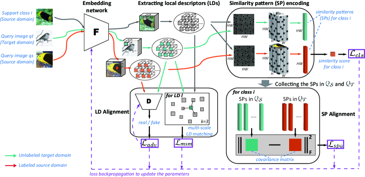
Figure 2. Illustration of our method performing episodic training for 5-way, 1-shot UDA tasks. In each episode, the support set $X_{\mathcal{S}}$ contains a photo image per support class, and the query sets ($Q_{\mathcal{S}}$ and $Q_{\mathcal{T}}$) contains the photo and sketch query images, respectively. Support class $i$ and query images $qs,qt$ from both domains are first through the feature embedding network $F$ to extract their local descriptors (LDs), followed by similarity pattern encoding module to learn similarity patterns (SPs). Then, we leverage the SPs in $Q_{\mathcal{S}}$ to calculate the similarity of query images to the class $i$ for classification loss $\mathcal{L}_{cls}$. Meanwhile, we calculate the covariance matrix of the SPs between $Q_{\mathcal{S}}$ and $Q_{\mathcal{T}}$ for measuring their domain alignment loss $\mathcal{L}_{spa}$. In addition, the LDs from both domains are further aligned by calculating both adversarial training loss $\mathcal{L}_{adv}$ and multi-scale matching loss $\mathcal{L}_{msm}$. Finally, the above losses are backpropagated to update the embedding model $F$.

3. Methodology

3.1. Problem Definition

A N-way, K-shot UDA task. Our FS-UDA setting involves two domains in total: a source domain $\mathcal{S}$ and a target domain $\mathcal{T}$. A N-way, K-shot UDA task includes a support set $X_{\mathcal{S}}$ from $\mathcal{S}$ and a query set $Q_{\mathcal{T}}$ from $\mathcal{T}$. The support set $X_{\mathcal{S}}$ contains $N$ classes and $K$ source domain samples per class. The query set $Q_{\mathcal{T}}$ contains the same $N$ classes as in $X_{\mathcal{S}}$ and $N_{q}$ target domain samples per class. To classify query images in $Q_{\mathcal{T}}$ to the correct class in $X_{S}$, as a conventional solution, leveraging the insufficient support set $X_{\mathcal{S}}$ to train a specific model from scratch could make the classification inefficient. Therefore, we aim to train a general model that can handle many new N-way, K-shot UDA tasks for testing. Table 2 shows the main symbols used in this paper.

Table 2. Notations.

Notations	Descriptions
$N,K\in\mathbb{R}$	The number of the classes and samples per class
$\lambda_{s},\lambda_{a},\lambda_{m}\in\mathbb{R}$	Weight parameters of three loss terms in Eq. (5)
$X_{\mathcal{S}},\mathcal{Q}_{\mathcal{S}},\mathcal{Q}_{\mathcal{T}}$	Support set of source domain, and query sets of
	source domain and target domain
$H,W,C\in\mathbb{R}$	The height, the width and the number of channels,
$l\in\mathbb{R}^{C}$	and local descriptor (LD) vector in the feature map
$L_{q}^{que}\in\mathbb{R}^{HW\times C}$	LD matrix that consists of LDs of a query image $q$,
$L_{c}^{sup}\in\mathbb{R}^{KHW\times C}$	LD matrix that consists of LDs of a support class $c$
$M_{q}^{c}\in\mathbb{R}^{HW\times KHW}$	2D and 3D matrices of cosine similarities between
$M_{q}^{c^{\prime}}\in\mathbb{R}^{H\times W\times KHW}$	LDs of a query image $q$ and a support class $c$
$p_{q}^{c}\in\mathbb{R}^{KHW}$	Similarity pattern (SP) vectors of a query image $q$
$p_{q}^{i}\in\mathbb{R}^{HW}$	to a support class $c$ and a support image $i$
$\Sigma_{d}^{i}\in\mathbb{R}^{HW\times HW}$	Covariance matrix of similarity patterns from all
	query images in domain $d$ to a support image $i$
$F,D$	Feature embedding network, domain discriminator

Auxiliary dataset and episodic training. Inspired by FSL, we resort to an auxiliary dataset $D^{\text{aux}}$ and perform episodic training to learn the general model. The auxiliary dataset $D^{\text{aux}}$ includes labeled source domain data and unlabeled target domain data. Note that, the classes in $D^{\text{aux}}$ are completely different from the testing N-way, K-shot UDA tasks. That is, the classes of the testing UDA tasks are unseen during episodic training. We construct large amounts of episodes to simulate the testing UDA tasks for task-level generalization (Vinyals et al., 2016). Each episode contains a support set $X_{\mathcal{S}}$, a source domain query set $Q_{\mathcal{S}}$ and a target domain query set $Q_{\mathcal{T}}$ sampled from $D^{\text{aux}}$. Specifically, in each episode, we randomly sample $N$ classes and $K+N_{q}$ source domain samples per class from $D^{\text{aux}}$. The $K+N_{q}$ samples per class are partitioned into $K$ in $X_{\mathcal{S}}$ and the remaining $N_{q}$ in $Q_{\mathcal{S}}$. Meanwhile, we randomly sample $N*N_{q}$ target domain samples (without considering labels) from $D^{\text{aux}}$ and incorporate them into $Q_{\mathcal{T}}$. Note that the query set $Q_{\mathcal{S}}$ per episode is additional, compared with the testing tasks. This is because the labels of $Q_{\mathcal{T}}$ are unavailable, we instead leverage $Q_{\mathcal{S}}$ to calculate classification loss, and meanwhile use $Q_{\mathcal{S}}$ and $Q_{\mathcal{T}}$ for domain alignment.

The flowchart of our method. Figure 2 illustrates our method to perform episodic training for 5-way, 1-shot UDA tasks. In each episode, a support set ($X_{\mathcal{S}}$) and two query sets ($Q_{\mathcal{S}}$ and $Q_{\mathcal{T}}$) are first through the feature embedding network $F$ to extract their LDs, followed by similarity encoding module to learn similarity patterns (SPs). Then, we leverage the SPs to calculate the image-to-class similarity for classification loss $\mathcal{L}_{cls}$. Meanwhile, we calculate the covariance matrix of the SPs between domains to measure their domain alignment loss $\mathcal{L}_{spa}$. In addition, the LDs from domains are further aligned by calculating both adversarial training loss $\mathcal{L}_{adv}$ and multi-scale matching loss $\mathcal{L}_{msm}$. Finally, the above losses are back-propagated to update the embedding model $F$. After episodic training over all episodes, we employ the learned embedding model $F$ to test many 5-way, 1-shot new UDA tasks. For each new testing task, the support set $X_{\mathcal{S}}$ is used to classify target domain samples in $Q_{\mathcal{T}}$. Then, we calculate the averaged classification accuracy on these tasks for performance evaluation.

3.2. Similarity Pattern Encoding

Inspired by LD-based FSL methods (Li et al., 2019a, 2020; Zhang et al., 2020), we employ plenty of local descriptors (LDs) to measure the image-to-class similarity. Considering spatial relationship of LDs, we believe that for two LDs that are spatially adjacent and therefore highly likely similar to each other, their similarity values to other LDs should be close and change in a smooth manner. However, the above methods did not effectively take this into account, and could generate noisy or non-smooth similarities with respect to the spatial dimension. Moreover, merely having a single similarity score as in the above methods cannot effectively serve the domain alignment required in our FS-UDA. Therefore, we propose a similarity encoding module to learn image-to-class similarity patterns (SPs), by leveraging Gaussian filter and max-pooling to smooth and aggregate the similarities of LDs. The learning process of SPs is cast into three following parts:

(1) Computing the similarity matrix of LDs (see step 1 in Figure 1) as in DN4 (Li et al., 2019a). We firstly extract the LDs of a query image $q$ and a support class $c\ (c=1,..,N)$, and then construct their LD matrix $L_{q}^{que}\in\mathbb{R}^{HW\times C}$ and $L_{c}^{sup}\in\mathbb{R}^{KHW\times C}$, respectively, where each row represents a LD vector. $H,\ W$ and $C$ denote the height, the width and the number of channels of the feature map, respectively. Then, we compute their cosine similarity matrix $M^{c}_{q}\in\mathbb{R}^{HW\times KHW}$ by $cos(L_{q}^{que},L_{c}^{sup})$. Finally, we only maintain the top-$k$ similarity values for each row in $M^{c}_{q}$ and set the remaining as zero.

(2) Reshaping the similarity matrix $M^{c}_{q}$ into a 3D map (see step 2 in Figure 1). To recover the spatial positions of query images in the similarity matrix, we reshape the similarity matrix $M^{c}_{q}$ into a 3D similarity representation $M^{c^{\prime}}_{q}\in\mathbb{R}^{H\times W\times KHW}$, by partitioning its first dimension $HW$ to the two dimensions $H$ and $W$.

(3) Performing Gaussian filter and max-pooling to generate the SPs (see step 3 in Figure 1). According to our observation, several noises or non-smooth values exist on the first two-dimensional plane of $M^{c^{\prime}}_{q}$. Considering that similarities of spatially-adjacent LDs to other LDs should be close, we conduct Gaussian filtering (with $3\times 3\times 1$ size) from the first two dimensions of $M^{c^{\prime}}_{q}$ to smooth their similarities. Then, max-pooling is employed to extract the discriminative similarity and finally generate the SP vectors $\{p^{c}_{q}\}$. Compared with a single similarity score used in (Li et al., 2019a), a SP contains the similarities of a query image to all LDs of the support class. Thus, the SP provides an informative and patterned measurement, which will be used for classification and domain alignment.

For classification, we calculate the image-to-class similarity score for each support class by summing all the elements of the SP vector, i.e. $\mathbf{1}^{\top}\cdot p^{c}_{q}$, and then select the class label with the highest score as the predicted label of query image $q$. The classification loss $\mathcal{L}_{cls}$ is calculated by cross-entropy loss, which can be written by:

(1) $$\mathcal{L}_{cls}=-\frac{1}{|Q_{\mathcal{S}}|}\sum_{q\in Q_{\mathcal{S}}}\log\frac{\exp(\mathbf{1}^{\top}\cdot p^{c^{*}}_{q})}{\sum_{c}\exp(\mathbf{1}^{\top}\cdot p^{c}_{q})},$$

where $c^{*}$ is the actual label of the query image $q$.

3.3. Similarity Pattern Alignment

To reduce the domain gap, we align the SPs of query images from the source and target domains, because the SPs contain image-to-class similarities that are crucial to final classification predictions. Considering that covariance matrix could exactly capture the underlying distribution information (Li et al., 2019b; He et al., 2019; Berthelot et al., 2017), we align the covariance matrix of the SPs from both domains for domain adaptation.

For fine-grained alignment, we focus on the SP between a query image $q$ and a specific support image $i$ (namely image-to-image SP, $p^{i}_{q}\in\mathbb{R}^{HW}$), instead of the image-to-class one. In other words, the learned image-to-class pattern $p^{c}_{q}\in\mathbb{R}^{KHW}$ can be decomposed into $K$ different image-to-image patterns $p^{i}_{q}\in\mathbb{R}^{HW\times 1},i=1,...,K$.

Specifically, for a support image $i$, we first collect its image-to-image SPs from all the query images in the source domain to form a set of SPs $\mathcal{E}^{i}_{\mathcal{S}}=\{p^{i}_{q}|q\in Q_{\mathcal{S}}\}$. Similarly, we also obtain the set of SPs in the target domain, i.e. $\mathcal{E}^{i}_{\mathcal{T}}=\{p^{i}_{q}|q\in Q_{\mathcal{T}}\}$. Then, the covariance matrix $\Sigma_{d}^{i}\in\mathbb{R}^{HW\times HW}$ for both domains ($d=\{\mathcal{S},\mathcal{T}\}$) can be calculated by $\Sigma_{d}^{i}=\frac{1}{|\mathcal{E}^{i}_{d}|-1}\mathop{\sum}_{p_{q}^{i}\in\mathcal{E}^{i}_{d}}(p_{q}^{i}-\bar{p}^{i})(p_{q}^{i}-\bar{p}^{i})^{\rm{T}}$, where $\bar{p}^{i}$ represents the averaged vector of SPs in the set $\mathcal{E}^{i}_{d}$. Finally, to align the two domains, we design a loss function of similarity pattern alignment (spa) to minimize the difference between $\Sigma_{\mathcal{S}}^{i}$ and $\Sigma_{\mathcal{T}}^{i}$, which can be calculated as:

(2) $$\mathcal{L}_{spa}(\{\Sigma_{\mathcal{S}}^{i}\},\{\Sigma_{\mathcal{T}}^{i}\})=\frac{1}{NK}\sum_{i=1}^{NK}||\Sigma_{\mathcal{S}}^{i}-\Sigma_{\mathcal{T}}^{i}||_{F}^{2},$$

where $NK$ represents the number of images in N-way, K-shot support set. By minimizing the loss $\mathcal{L}_{spa}$, the domain gap will be reduced. In some sense, this loss can also be viewed as a regularization of image-to-class similarity measurement. This will be also validated in the experiments of few-shot learning.

3.4. Local Descriptor Alignment

Domain Adversarial Module. To align the domains on local features, we apply adversarial training on the LDs of query images between $Q_{\mathcal{S}}$ and $Q_{\mathcal{T}}$, which are from the distributions $P_{\mathcal{S}}$ and $P_{\mathcal{T}}$, respectively. We design a domain discriminator $D$ to predict the domain label of each LD $l\in\mathbb{R}^{C}$. The adversarial training loss can be written by:

(3) $$\min_{F}\max_{D}\mathcal{L}_{adv}=\mathop{\rm{E}}_{l\sim P_{\mathcal{S}}}[\log(1-D(l))]+\mathop{\rm{E}}_{l\sim P_{\mathcal{T}}}[\log D(l)]$$

In each episode, we minimize the loss $\mathcal{L}_{adv}$ for the embedding network $F$ and maximize the loss for the discriminator $D$.

Multi-scale Local Descriptor Matching. In addition, to incorporate the discriminative information of LDs in the target domain for domain alignment, we develop a multi-scale local descriptor matching (msm) module between domains. It is encouraged to push each LD $l$ in $Q_{\mathcal{T}}$ to its $k$ ($k>1$) nearest neighbors from multi-scale LDs in $X_{\mathcal{S}}$ in an unsupervised way. These multi-scale LDs are generated by average pooling on embedded feature maps with different scales ($5\times 5,2\times 2,1\times 1$), and cosine similarity is utilized to find the nearest neighbors. This loss can be written as:

(4) $$\mathcal{L}_{msm}=-\frac{1}{|Q_{\mathcal{T}}|}\sum_{q\in Q_{\mathcal{T}}}\sum_{l\in q}\sum_{i=1}^{k}\log\frac{\exp(m_{l}^{i})}{\sum_{j=1}^{n}\exp(m_{l}^{j})},$$

where $m_{l}^{j}\in[-1,1]$ represents the cosine similarity of the LD $l$ to its $j$-th neighbor in multi-scale LDs of $X_{\mathcal{S}}$. Also, for every query image, we only measure the similarity of its $n$ neighbors, and the remaining neighbors are not considered.

In sum, we combine the above losses to train the feature embedding network $F$ on a large amount of episodes. The overall objective function can be written as:

(5) $$\min_{F}\max_{D}[\mathcal{L}_{cls}+\lambda_{s}\mathcal{L}_{spa}+\lambda_{a}\mathcal{L}_{adv}+\lambda_{m}\mathcal{L}_{msm}],$$

where the parameters $\lambda_{s},\lambda_{a}$ and $\lambda_{m}$ are to balance the effects of different loss terms $\mathcal{L}_{spa},\mathcal{L}_{adv}$ and $\mathcal{L}_{msm}$, respectively. The whole process of the proposed IMSE is summarized in Algorithm 1.

Algorithm 1 Proposed IMSE

Training Input: An auxiliary dataset $D^{\text{aux}}$ including labeled
source and unlabeled target domain data, parameters $\lambda_{s},\lambda_{a},\lambda_{m}$
Training Output: Embedding network $F$ and discriminator $D$

1:  Randomly initialize $F$ and $D$.

2:  while not converged do

3:     Sample an episode $\{X_{\mathcal{S}},\mathcal{Q}_{\mathcal{S}},\mathcal{Q}_{\mathcal{T}}\}$ from $D^{\text{aux}}$.

4:     # compute similarity patterns

5:     Calculate similarity patterns $\{p_{q}^{c}|q\in\mathcal{Q}_{\mathcal{S}}\bigcup\mathcal{Q}_{\mathcal{T}},c=1,...,N\}$ using $F(X_{\mathcal{S}})$, $F(\mathcal{Q}_{\mathcal{S}})$ and $F(\mathcal{Q}_{\mathcal{T}})$.

6:     # compute classification loss and domain alignment losses

7:     Compute classification loss $\mathcal{L}_{cls}$ for labeled query set $\mathcal{Q}_{\mathcal{S}}.$

8:     Compute SP alignment loss $\mathcal{L}_{spa}$ via Eq. (2).

9:     Compute LD alignment losses $L_{adv},L_{msm}$ via Eqs. (3)-(4).

10:     # update parameters

11:     Optimize the $F$ and $D$ by minimizing the objective in Eq. (5).

12:  end while

Testing Input: New tasks and trained embedding network $F$
Testing Output: Predictions $\{\hat{y}_{q}\}$ in target domain of new tasks

1:  for  $\{X_{\mathcal{S}},\mathcal{Q}_{\mathcal{T}}\}$ in new tasks do

2:     # test on a new task

3:     Compute similarity patterns $\{p_{q}^{c}|q\in\mathcal{Q}_{\mathcal{T}},c=1,...,N\}$ using $F(X_{\mathcal{S}})$ and $F(\mathcal{Q}_{\mathcal{T}})$.

4:     Predict the labels $\{\hat{y}_{q}\}$, $\hat{y}_{q}={\arg\max}_{c}\{\mathbf{1}^{\top}\cdot p^{c}_{q}|c=1,...,N\}$.

5:  end for

4. Experiments

DomainNet dataset. To demonstrate the efficacy of our method, we conduct extensive experiments on a multi-domain benchmark dataset DomainNet. It was released in 2019 for the research of multi-source domain adaptation (Peng et al., 2019). It contains 345 categories and six domains per category, i.e. quickdraw, clipart, real, sketch, painting, infograph domains. In our experiments, we first remove the data-insufficient domain infograph, and select any two from the remaining five domains as the source and target domains. Thus, we have 20 combinations totally for evaluation. Then, we discard the 37 categories that contain less than 20 images for the five domains. Finally, we randomly split the images of the remaining 308 categories into the images of 217 categories, 43 categories and 48 categories for episodic training (forming the auxiliary dataset), model validation and testing new tasks, respectively. Note that in each split every category contains the images of the five domains.

Network architecture. We employ ResNet-12 as the backbone of the embedding network, which is widely used in few-shot learning (Chen et al., 2020). As for similarity pattern encoder, we set a $3\times 3\times 1$ Gaussian kernel with standard deviation $0.8$ and stride $1$. Then, a $2\times 2$ max-pooling with stride $2$ is conducted. As for adversarial training, we use three fully-connected layers to build a domain discriminator.

Model training. Before episodic training, inspired by (Chen et al., 2020), a pre-trained the embedding network is trained by source domain data in the auxiliary dataset, which is used for performance improvement. Specifically, we first train the ResNet-12 with a full-connected layer to classify the source domain images in the auxiliary dataset. After the pre-training, we remove the full-connected layer and retain the convolutional blocks of ResNet-12 as the initialized model of the episodic training. Afterwards, we perform episodic training on 10000 episodes. For each episode, we randomly sample a support set (including 5 categories, and 1 or 5 source domain samples per category) and a query set (including 15 source domain samples for each of the same 5 categories and 75 randomly sampled target domain samples). During episode training, the total loss in Eq. (5) is minimized to optimize the network parameters for each episode. Also, we employ Adam optimizer with an initial learning rate of $1e\text{-}4$, and reduce the learning rate by half every 1000 episodes.

Model validation and testing. For model validation, we compare the performance of different model parameters on 3000 tasks, which is randomly sampled from the validate set containing 43 categories. Then, we select the model parameters with the best validation accuracy for testing. During the testing phase, we randomly construct 3000 new FS-UDA tasks from the testing set containing 48 categories. For each task, the support set includes 5 categories, and 1 or 5 source domain samples per category, and the query set only includes 75 target domain samples from the same 5 categories for evaluation. The averaged top-1 accuracy on the 3000 tasks is calculated as the evaluation criterion.

Table 3. Comparison of our method with the UDA, FSL and their combination methods for 5-way 1-shot or 5-shot FS-UDA tasks. Each row represents the accuracy (%) of a compared method adapting between two domains, where the skt, rel, qdr, pnt, and cli denote the sketch, real, quickdraw, painting, and clipart domains in the DomainNet dataset, respectively. The best results are in bold.

5-way, 1-shot
Methods	skt$\leftrightarrow$rel	skt$\leftrightarrow$qdr	skt$\leftrightarrow$pnt	skt$\leftrightarrow$cli	rel$\leftrightarrow$qdr	rel$\leftrightarrow$pnt	rel$\leftrightarrow$cli	qdr$\leftrightarrow$pnt	qdr$\leftrightarrow$cli	pnt$\leftrightarrow$cli	avg
	$\rightarrow$ / $\leftarrow$	$\rightarrow$ / $\leftarrow$	$\rightarrow$ / $\leftarrow$	$\rightarrow$ / $\leftarrow$	$\rightarrow$ / $\leftarrow$	$\rightarrow$ / $\leftarrow$	$\rightarrow$ / $\leftarrow$	$\rightarrow$ / $\leftarrow$	$\rightarrow$ / $\leftarrow$	$\rightarrow$ / $\leftarrow$	–
MCD (Saito et al., 2018)	48.07/37.74	38.90/34.51	39.31/35.59	51.43/38.98	24.17/29.85	43.36/47.32	44.71/45.68	26.14/25.02	42.00/34.69	39.49/37.28	38.21
ADDA (Tzeng et al., 2017)	48.82/46.06	38.42/40.43	42.52/39.88	50.67/47.16	31.78/35.47	43.93/45.51	46.30/47.66	26.57/27.46	46.51/32.19	39.76/41.24	40.91
DWT (Roy et al., 2019)	49.43/38.67	40.94/38.00	44.73/39.24	52.02/50.69	29.82/29.99	45.81/50.10	52.43/51.55	24.33/25.90	41.47/39.56	42.55/40.52	41.38
ProtoNet (Snell et al., 2017)	50.48/43.15	41.20/32.63	46.33/39.69	53.45/48.17	32.48/25.06	49.06/50.30	49.98/51.95	22.55/28.76	36.93/40.98	40.13/41.10	41.21
DN4 (Li et al., 2019a)	52.42/47.29	41.46/35.24	46.64/46.55	54.10/51.25	33.41/27.48	52.90/53.24	53.84/52.84	22.82/29.11	36.88/43.61	47.42/43.81	43.61
ADM (Li et al., 2020)	49.36/42.27	40.45/30.14	42.62/36.93	51.34/46.64	32.77/24.30	45.13/51.37	46.8/50.15	21.43/30.12	35.64/43.33	41.49/40.02	40.11
FEAT (Ye et al., 2020)	51.72/45.66	40.29/35.45	47.09/42.99	53.69/50.59	33.81/27.58	52.74/53.82	53.21/53.31	23.10/29.39	37.27/42.54	44.15/44.49	43.14
DeepEMD (Zhang et al., 2020)	52.24/46.84	42.12/34.77	46.64/43.89	55.10/49.56	34.28/28.02	52.73/53.26	54.25/54.91	22.86/28.79	37.65/42.92	44.11/44.38	43.46
ADDA+ProtoNet	51.30/43.43	41.79/35.40	46.02/41.40	52.68/48.91	37.28/27.68	50.04/49.68	49.83/52.58	23.72/32.03	38.54/44.14	41.06/41.59	42.45
ADDA+DN4	53.04/46.08	42.64/36.46	46.38/47.08	54.97/51.28	34.80/29.84	53.09/54.05	54.81/55.08	23.67/31.62	42.24/45.24	46.25/44.40	44.65
ADDA+ADM	51.87/45.08	43.91/32.38	47.48/43.37	54.81/51.14	35.86/28.15	48.88/51.61	49.95/54.29	23.95/33.30	43.59/48.21	43.52/43.83	43.76
ADDA+FEAT	52.72/46.08	47.00/36.94	47.77/45.01	56.77/52.10	36.32/30.50	49.14/52.36	52.91/53.86	24.76/35.38	44.66/48.82	45.03/45.92	45.20
ADDA+DeepEMD	53.98/47.55	44.64/36.19	46.29/45.14	55.93/50.45	37.47/30.14	52.21/53.32	54.86/54.80	23.46/32.89	39.06/46.76	45.39/44.65	44.75
IMSE (ours)	57.21/51.30	49.71/40.91	50.36/46.35	59.44/54.06	44.43/36.55	52.98/55.06	57.09/57.98	30.73/38.70	48.94/51.47	47.42/46.52	48.86
5-way, 5-shot
MCD (Saito et al., 2018)	66.42/47.73	51.84/39.73	54.63/47.75	72.17/53.23	28.02/33.98	55.74/66.43	56.80/63.07	28.71/29.17	50.46/45.02	53.99/48.24	49.65
ADDA (Tzeng et al., 2017)	66.46/56.66	51.37/42.33	56.61/53.95	69.57/65.81	35.94/36.87	58.11/63.56	59.16/65.77	23.16/33.50	41.94/43.40	55.21/55.86	51.76
DWT (Roy et al., 2019)	67.75/54.85	48.59/40.98	55.40/50.64	69.87/59.33	36.19/36.45	60.26/68.72	62.92/67.28	22.64/32.34	47.88/50.47	49.76/52.52	51.74
ProtoNet (Snell et al., 2017)	65.07/56.21	52.65/39.75	55.13/52.77	65.43/62.62	37.77/31.01	61.73/66.85	63.52/66.45	20.74/30.55	45.49/55.86	53.60/52.92	51.80
DN4 (Li et al., 2019a)	63.89/51.96	48.23/38.68	52.57/51.62	62.88/58.33	37.25/29.56	58.03/64.72	61.10/62.25	23.86/33.03	41.77/49.46	50.63/48.56	49.41
ADM (Li et al., 2020)	66.25/54.20	53.15/35.69	57.39/55.60	71.73/63.42	44.61/24.83	59.48/69.17	62.54/67.39	21.13/38.83	42.74/58.36	56.34/52.83	52.78
FEAT (Ye et al., 2020)	67.91/58.56	52.27/40.97	59.01/55.44	69.37/65.95	40.71/28.65	63.85/71.25	65.76/68.96	23.73/34.02	42.84/53.56	57.95/54.84	53.78
DeepEMD (Zhang et al., 2020)	67.96/58.11	53.34/39.70	59.31/56.60	70.56/64.60	39.70/29.95	62.99/70.93	65.07/69.06	23.86/34.34	45.48/53.93	57.60/55.61	53.93
ADDA+ProtoNet	66.11/58.72	52.92/43.60	57.23/53.90	68.44/61.84	45.59/38.77	60.94/69.47	66.30/66.10	25.45/41.30	46.67/56.22	58.20/52.65	54.52
ADDA+DN4	63.40/52.40	48.37/40.12	53.51/49.69	64.93/58.39	36.92/31.03	57.08/65.92	60.74/63.13	25.36/34.23	48.52/51.19	52.16/49.62	50.33
ADDA+ADM	64.64/54.65	52.56/33.42	56.33/54.85	70.70/63.57	39.93/27.17	58.63/68.70	61.96/67.29	21.91/39.12	41.96/59.03	55.57/53.39	52.27
ADDA+FEAT	67.80/56.71	60.33/43.34	57.32/58.08	70.06/64.57	44.13/35.62	62.09/70.32	57.46/67.77	29.08/44.15	49.62/63.38	57.34/52.13	55.56
ADDA+DeepEMD	68.52/59.28	56.78/40.03	58.18/57.86	70.83/65.39	42.63/32.18	63.82/71.54	66.51/69.21	26.89/42.33	47.00/57.92	57.81/55.23	55.49
IMSE (ours)	70.46/61.09	61.57/46.86	62.30/59.15	76.13/67.27	53.07/40.17	64.41/70.63	67.60/71.76	33.44/48.89	53.38/65.90	61.28/56.74	59.60

Table 4. Ablation study of Gaussian kernel and max-pooling used in our IMSE to generate SPs.

Filters	Poolings	skt$\leftrightarrow$rel	skt$\leftrightarrow$qdr	skt$\leftrightarrow$pnt	skt$\leftrightarrow$cli	rel$\leftrightarrow$qdr	rel$\leftrightarrow$pnt	rel$\leftrightarrow$cli	qdr$\leftrightarrow$pnt	qdr$\leftrightarrow$cli	pnt$\leftrightarrow$cli	avg
		$\rightarrow$ / $\leftarrow$	$\rightarrow$ / $\leftarrow$	$\rightarrow$ / $\leftarrow$	$\rightarrow$ / $\leftarrow$	$\rightarrow$ / $\leftarrow$	$\rightarrow$ / $\leftarrow$	$\rightarrow$ / $\leftarrow$	$\rightarrow$ / $\leftarrow$	$\rightarrow$ / $\leftarrow$	$\rightarrow$ / $\leftarrow$	–
Gaussian	MaxPooling	57.21/51.30	49.71/40.91	50.36/46.35	59.44/54.06	44.43/36.55	52.98/55.06	57.09/57.98	30.73/38.70	48.94/51.47	47.42/46.52	48.86
Gaussian	DownSampling	50.01/42.72	34.11/30.62	37.71/33.47	51.91/43.78	36.22/26.30	41.18/45.33	49.41/48.43	23.61/31.30	36.06/43.63	35.40/33.73	38.74
Average	MaxPooling	40.81/40.23	37.54/28.81	35.51/32.93	40.10/37.16	34.79/24.62	37.73/40.35	41.32/40.91	21.48/30.32	34.74/44.50	33.16/31.97	35.44
None	MaxPooling	34.48/30.24	26.32/24.48	27.62/30.39	32.87/28.86	28.76/22.73	31.82/34.54	31.39/31.45	21.20/25.57	24.82/29.72	29.22/26.95	28.67

4.1. Comparison Experiments for FS-UDA

We conduct extensive experiments on DomainNet to compare our method with related FSL, UDA, and their combination methods.

UDA methods. We choose MCD (Saito et al., 2018), ADDA (Tzeng et al., 2017) and DWT (Roy et al., 2019) to compare with our method. Specifically, 1) we first train the UDA models by using all training categories in the auxiliary set; 2) Secondly, we replace the last classification layer of the models with a new 5-way classifier for various tasks, as in baseline++ (Chen et al., 2019); 3) Thirdly, for testing on each task, we freeze the trained backbone and only fine-tune the classifier for a novel task with its support set, by using an SGD optimizer (learning rate $0.01$, momentum $0.9$ and weight decay $1e\text{-}4$) with batch size $4$ for $300$ iterations. Finally, we test the classification performance on its query set.

FSL methods. Since our method is related to metric-based FSL methods, we choose five representative metric-based methods, i.e. ProtoNet (Snell et al., 2017), DN4 (Li et al., 2019a), ADM (Li et al., 2020), FEAT (Ye et al., 2020), and DeepEMD (Zhang et al., 2020) for comparisons. Especially, DN4, ADM and DeepEMD also utilize local descriptors for classification. For fair comparison, we also pre-train the embedding network and perform episodic training on auxiliary dataset (Chen et al., 2020). Note that, FSL methods don’t handle the domain shift between the support and query sets, and are also not capable of leveraging the target domain data in the auxiliary dataset because of no labels in the target domain. Thus, we further combine the FSL and UDA methods for domain adaptation and classification.

FSL methods combined with ADDA (Tzeng et al., 2017). We combine the five above FSL methods with ADDA (Tzeng et al., 2017), which are abbreviated as ADDA+ProtoNet, ADDA+DN4, ADDA+ADM, ADDA+FEAT, and ADDA+DeepEMD, respectively. Specifically, we add the feature-level adversarial loss in ADDA (Tzeng et al., 2017) for domain alignment in every episode. The used discriminator is the same with our method. For fair comparison, these combination methods also pretrain the embedding network before episodic training.

Comparison Analysis. Table 3 shows the results of all the compared methods for 20 cross-domain combinations, which records the averaged classification accuracy of target domain samples over 3000 5-way 1-shot/5-shot UDA tasks. As reported in Table 3, our IMSE achieves the best performance for the most combinations and their average. Specifically, the UDA and FSL baselines in the first two parts of Table 3 perform much worse than our method. This is because the UDA models did not consider task-level generalization, and the FSL models are lack of handling domain shift. In the third part of Table 3, the combination methods we build perform domain adversarial training over every episode. They are thus generally better than the above two parts, but still inferior to our IMSE. This is because the combination methods with ADDA (Tzeng et al., 2017) only perform the domain alignment based on feature maps, not considering the alignment of both local descriptors (more fine-grained than feature maps) and similarity patterns (related to classification predictions) used in our IMSE. This shows the efficacy of our IMSE for FS-UDA.

On the other hand, we can see that the 20 cross-domain combinations have considerably different performances. This is because several domains (e.g. quickdraw) are significantly different from other domains, while some other domains (e.g. real, painting) are with the similar styles and features. Thus, the performance becomes relatively low when large domain gap is presented, and the situation will become better when the domain gap reduces. For example, from quickdraw to painting/real, most methods perform worse due to larger domain gap, but our IMSE and ADDA (Tzeng et al., 2017) perform much better than the others, showing the positive effect of their domain alignment. From painting to real and real to painting which have smaller domain gap, the FSL, combinational methods and our IMSE perform better than the UDA methods, showing the positive effect of task generalization. In general, this reflects the advantages of our IMSE to deal with domain shift and task generalization in FS-UDA, especially for large domain gap.

Evaluation on FSL methods with our domain alignment modules. To further validate the efficacy of the two alignment modules designed in our IMSE, i.e. similarity pattern alignment and local descriptor alignment, we incorporate their corresponding loss terms $\mathcal{L}_{spa}$, $\mathcal{L}_{adv}$ and $\mathcal{L}_{msm}$ into the loss functions of three FSL models ProtoNet, DeepEMD and DN4, namely IMSE+ProtoNet, IMSE+DeepEMD and IMSE+DN4, respectively. We test them on 3000 new FS-UDA tasks, compared with the FSL methods (ProtoNet, DeepEMD and DN4) and the combination methods with ADDA (Tzeng et al., 2017) (ADDA+ProtoNet, ADDA+DeepEMD and ADDA+DN4). For simplification and clarification, we average the accuracy from every domain to the other four domains, which are shown in Figure 3. Obviously, these methods IMSE+ProtoNet, IMSE+DeepEMD and IMSE+DN4 are more significantly improved by using our alignment modules in IMSE, which indicates the effectiveness of aligning the SPs and LDs again. Moreover, these methods are still outperformed by our IMSE, because we have a complete and self-contained FS-UDA framework, and the designed similarity patterns are effective for classification. This shows the efficacy of our IMSE again.

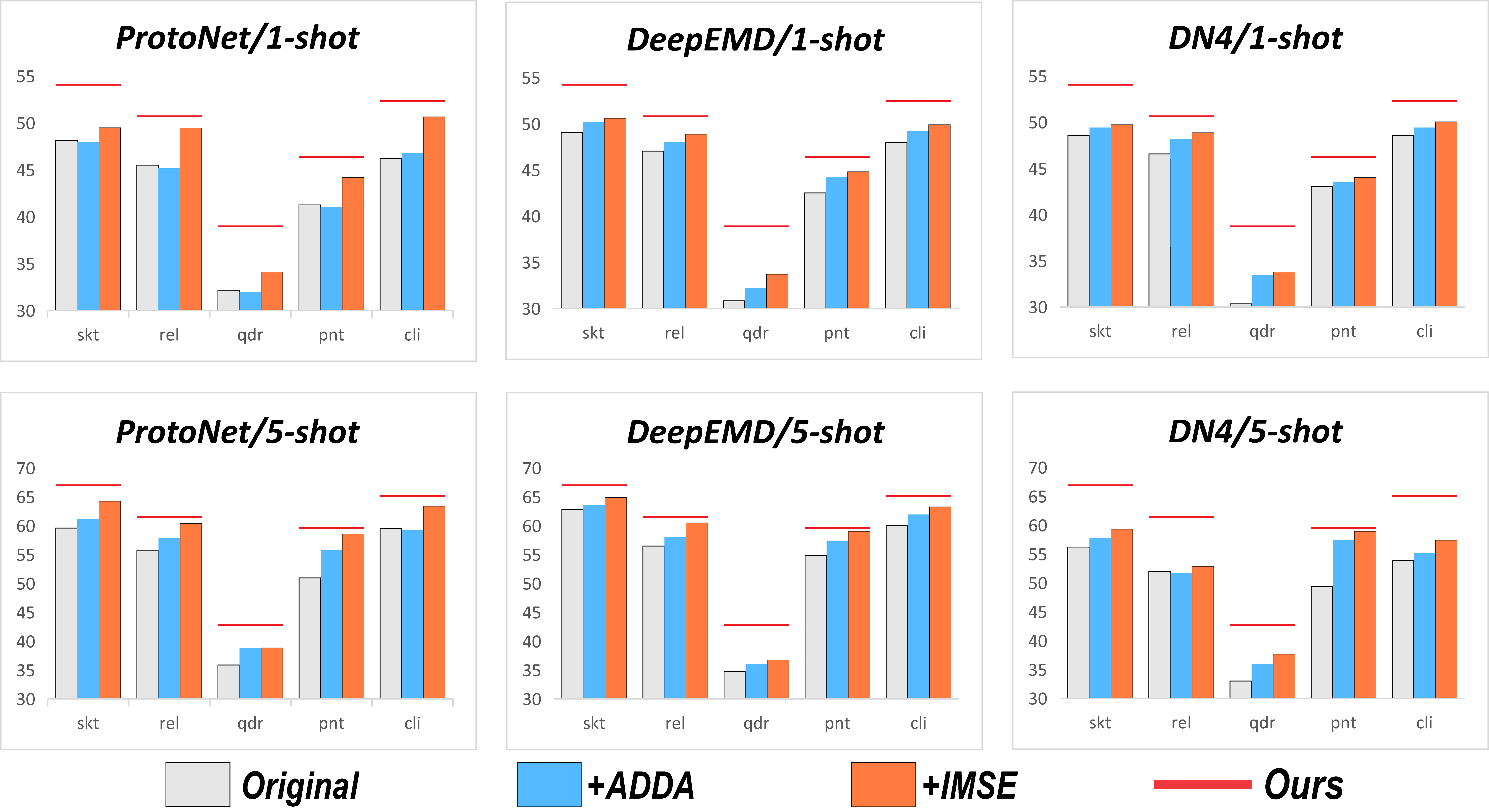
Figure 3. Comparison of applying different domain alignment modules to three FSL methods ProtoNet, DeepEMD and DN4. The red lines denote the accuracy of our method.

Different losses. We conduct various experiments on DomainNet to further evaluate the effect of our different losses in Eq.(5). Besides the classification loss ($\mathcal{L}_{cls}$), we combine the remaining three loss terms: 1) LD adversarial training loss ($\mathcal{L}_{adv}$), 2) multi-scale LD matching loss ($\mathcal{L}_{msm}$), and 3) similarity pattern alignment loss ($\mathcal{L}_{spa}$). We evaluate both 1-shot and 5-shot FS-UDA tasks by taking sketch as the source domain, and the other four domains as the target domains, respectively. The accuracies on the four target domains are reported in Table 5. As observed, the more the number of loss terms involved, the higher the accuracy. The combination of all the three losses is the best. For the single loss, $\mathcal{L}_{spa}$ performs better than $\mathcal{L}_{adv}$ and $\mathcal{L}_{msm}$, showing the efficacy of SP alignment. The combination of $\mathcal{L}_{adv}$ and $\mathcal{L}_{msm}$ is considerably better than either one of them, showing the positive effect of combining multi-scale LD matching and LD adversarial training. Based on the above, the addition of $\mathcal{L}_{spa}$ further improves the performance, indicating the necessity of jointly aligning SPs and LDs.

Gaussian kernel and maxpooling for SPs. We further investigate the process of generating our SPs by applying Gaussian kernel and maxpooling (see Figure 1). We try to change the filters and the poolings, and compare the variants in Table 4. As seen, our method in the first row performs best. The performance decreases sharply when Gaussian filter is replaced or removed (see rows 3-4 in Table 4). This is because Gaussian kernel efficiently makes the similarity of adjacent points smooth. For downsampling in the second row, we remove the maxpooling and perform the downsampling by changing the filter stride to 2, but it performs worse than our IMSE using maxpooling in the first row. This is because maxpooling extracts local maximum responses of similarity maps that could reflect the prominent and discriminative characteristics for classification.

Table 5. Ablation study of the three losses designed in our IMSE, where the FS-UDA tasks are evaluated from a source domain (skt) to four different target domains (rel, qdr, pnt, and cli) in DomainNet.

Components			Target Domains
$\mathcal{L}_{adv}$	$\mathcal{L}_{msm}$	$\mathcal{L}_{spa}$	rel	qdr	pnt	cli
			54.42	42.28	46.80	56.37
✓			52.11	44.51	48.76	56.99
	✓		54.53	42.10	47.62	56.58
		✓	56.12	48.37	49.44	58.78
✓	✓		55.30	45.52	49.53	58.34
✓		✓	56.57	49.03	50.17	59.12
	✓	✓	56.00	47.93	50.13	58.33
✓	✓	✓	57.21	49.71	50.36	59.30

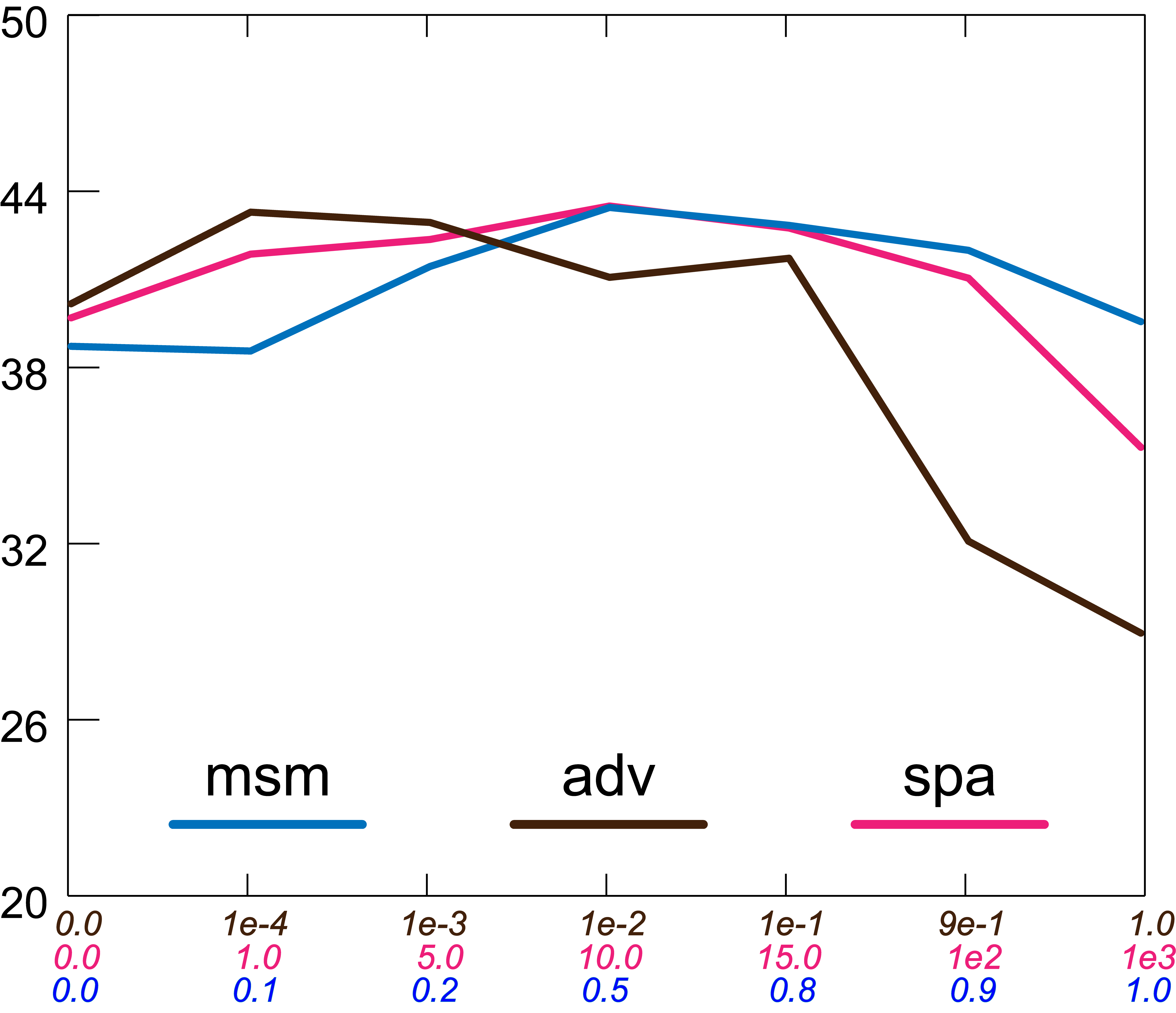
Figure 4. Sensitivity of $\lambda_{a}$, $\lambda_{s}$ and $\lambda_{m}$ for rel$\rightarrow$qdr.

Table 6. Cross-dataset evaluation for 5-way 1-shot UDA tasks between two domains rel and skl: performing episodic training on DomainNet, and testing on expanded dataset miniImageNet*.

Methods	skl$\rightarrow$rel	rel$\rightarrow$skl
DN4	44.01$\pm$0.87	40.61$\pm$0.90
DeepEMD	46.14$\pm$0.82	45.91$\pm$0.77
IMSE (ours)	48.78$\pm$0.78	48.52$\pm$0.81

Cross-dataset evaluation. We investigate the performance of our model on a substantially different dataset miniImageNet, after episodic training on DomainNet. To produce two domains for FS-UDA, we modify miniImageNet by transferring a half of real images (rel) into sketch images (skt) by MUNIT (Huang et al., 2018). We conduct experiments between rel and skt, and compare our IMSE with DN4 and DeepEMD for 5-way 1-shot UDA tasks. Their accuracies are shown in Table 4. As seen, our method still performs better than DN4 and DeepEMD, showing the efficacy of our IMSE again. Compared with DomainNet, the results in miniImageNet have some performance degeneration, since their sketch images are more simplified than that in DomainNet, and thus have larger difference from real images.

Hyper-parameters sensitive analysis. To investigate the effect of three domain alignment losses, we conduct the sensitive experiments of three hyper-parameters in Eq. (5), i.e. $\lambda_{a}$, $\lambda_{s}$ and $\lambda_{m}$, respectively. We fix two parameters as the optimal values, and meanwhile change the other one for performance evaluation. The changing accuracy curves of the three parameters are shown in Figure 4. Obviously, the curves of the parameters $\lambda_{s}$ and $\lambda_{m}$ are stably changing. When $\lambda_{a}$ is less than $0.1$, it also changes slowly. This shows the low sensitivity of the three parameters.

Table 7. Comparison with the FSL baselines using the backbone ResNet-12 on miniImageNet. The top two results are in bold.

Method	1-shot	5-shot
ProtoNet (Snell et al., 2017)	60.37 $\pm$ 0.83	78.02 $\pm$ 0.57
MTL (Sun et al., 2019)	61.20 $\pm$ 1.80	75.50 $\pm$ 0.80
MatchNet (Vinyals et al., 2016)	63.08 $\pm$ 0.80	75.99 $\pm$ 0.60
TADAM (Oreshkin et al., 2018)	58.50 $\pm$ 0.30	76.70 $\pm$ 0.30
DN4 (Li et al., 2019a)	61.57 $\pm$ 0.72	71.40 $\pm$ 0.61
CAN (Hou et al., 2019)	63.85 $\pm$ 0.48	79.44 $\pm$ 0.34
DeepEMD (Zhang et al., 2020)	65.91 $\pm$ 0.82	82.41 $\pm$ 0.56
IMSE w/o $\mathcal{L}_{rspa}$	62.46 $\pm$ 0.87	78.44 $\pm$ 0.47
IMSE (ours)	65.35 $\pm$ 0.42	80.02 $\pm$ 0.34

4.2. Few-shot learning on miniImageNet

Additionally, we investigate the performance of our IMSE for few-shot learning with 1-shot and 5-shot setting on a benchmark dataset miniImageNet. We adopt the same data partitioning, training and testing setting as in (Li et al., 2019a). Since in few-shot learning the support and query sets are from the same domain, only one domain exists and no domain alignment is required in this experiment. Thus, we discard the LD-based domain alignment losses $\mathcal{L}_{adv}$ and $\mathcal{L}_{msm}$ used in our method, and retain the classification loss $\mathcal{L}_{cls}$. Meanwhile, we modify the similarity pattern (SP) alignment loss $\mathcal{L}_{spa}$ to constrain the covariance matrix of SPs to be an identity matrix: $\mathcal{L}_{rspa}(\{\Sigma^{i}\})=\frac{1}{NK}\sum_{i=1}^{NK}||\Sigma^{i}-\lambda\cdot I_{HM}||_{F}^{2}$, where $\lambda=\frac{1}{HW}tr(\Sigma^{i})$. It can be viewed as a regularizer to learn less biased SPs for classification.

We compare our method with seven representative FSL methods in Table 7. The results of almost all the compared methods are quoted from (Zhang et al., 2020), except CAN and DN4. The results of CAN are quoted from its original work (Hou et al., 2019). Since DN4 in (Li et al., 2019a) did not use backbone ResNet-12 (our setting), we use its released code, the backbone ResNet-12 and pretraining to do experiments for a fair comparison. Note that, we compare the FC version of DeepEMD, because it has no data augmentation, neither ours. Also, we evaluate IMSE by using the loss $\mathcal{L}_{rspa}$ or not. As observed in Table 7, IMSE performs better than most of recent FSL methods, showing excellent performance of IMSE for FSL. Meanwhile, our method is slightly lower than DeepEMD, especially for 5-shot. This may be because DeepEMD needs to learn new prototypes for each testing 5-shot task, which could improve the performance but is more time-consuming than ours. In addition, in our IMSE, it is much better to use the $\mathcal{L}_{rspa}$ than to remove it, which indicates the positive effect of using covariance matrix of SPs as regularization.

5. Conclusion

In this paper, we propose a novel method IMSE for the new setting of FS-UDA. Our IMSE leverages local descriptors to design the similarity patterns to measure the similarity of query images and support classes from different domains. To learn a domain-shared embedding model for FS-UDA, we align the local descriptors by adversarial training and multi-scale matching, and align the covariance matrices of the similarity patterns. Extension experiments over DomainNet show the efficacy of our IMSE for FS-UDA, and our method also has good performance for FSL on miniImageNet.

- (1)
- Berthelot et al. (2017) David Berthelot, Tom Schumm, and Luke Metz. 2017. BEGAN: Boundary Equilibrium Generative Adversarial Networks. CoRR (2017). arXiv:1703.10717
- Bertinetto et al. (2019) Luca Bertinetto, João F. Henriques, Philip H. S. Torr, and Andrea Vedaldi. 2019. Meta-learning with Differentiable Closed-form Solvers. In ICLR.
- Cao et al. (2018) Yue Cao, Mingsheng Long, and Jianmin Wang. 2018. Unsupervised Domain Adaptation with Distribution Matching Machines. In AAAI. 2795–2802.
- Chen et al. (2019) Wei-Yu Chen, Yen-Cheng Liu, Zsolt Kira, Yu-Chiang Frank Wang, and Jia-Bin Huang. 2019. A Closer Look at Few-shot Classification. In ICLR.
- Chen et al. (2020) Yinbo Chen, Xiaolong Wang, Zhuang Liu, Huijuan Xu, and Trevor Darrell. 2020. A New Meta-baseline for Few-shot Learning. CoRR (2020). arXiv:2003.04390
- Finn et al. (2017) Chelsea Finn, Pieter Abbeel, and Sergey Levine. 2017. Model-agnostic Meta-learning for Fast Adaptation of Deep Networks. In ICML. 1126–1135.
- Ganin et al. (2016) Yaroslav Ganin, Evgeniya Ustinova, Hana Ajakan, Pascal Germain, Hugo Larochelle, François Laviolette, Mario Marchand, and Victor Lempitsky. 2016. Domain-adversarial Training of Neural Networks. J. Mach. Learn. Res 17, 1 (2016), 2096–2030.
- He et al. (2019) Ran He, Xiang Wu, Zhenan Sun, and Tieniu Tan. 2019. Wasserstein CNN: Learning Invariant Features for NIR-VIS Face Recognition. Trans. Pattern Anal. Mach. Intell. (2019), 1761–1773.
- Hou et al. (2019) Ruibing Hou, Hong Chang, Bingpeng Ma, Shiguang Shan, and Xilin Chen. 2019. Cross Attention Network for Few-shot Classification. In NIPS. 4005–4016.
- Hu et al. (2020) Lanqing Hu, Meina Kan, Shiguang Shan, and Xilin Chen. 2020. Unsupervised Domain Adaptation with Hierarchical Gradient Synchronization. In CVPR. 4042–4051.
- Huang et al. (2018) Xun Huang, Ming-Yu Liu, Serge J. Belongie, and Jan Kautz. 2018. Multimodal Unsupervised Image-to-Image Translation. In ECCV. 172–189.
- Li et al. (2020) Wenbin Li, Lei Wang, Jing Huo, Yinghuan Shi, Yang Gao, and Jiebo Luo. 2020. Asymmetric Distribution Measure for Few-shot Learning. In IJCAI. 2957–2963.
- Li et al. (2019a) Wenbin Li, Lei Wang, Jinglin Xu, Jing Huo, Yang Gao, and Jiebo Luo. 2019a. Revisiting Local Descriptor based Image-to-class Measure for Few-shot Learning. In CVPR. 7260–7268.
- Li et al. (2019b) Wenbin Li, Jinglin Xu, Jing Huo, Lei Wang, Yang Gao, and Jiebo Luo. 2019b. Distribution Consistency based Covariance Metric Networks for Few-shot Learning. In AAAI. 8642–8649.
- Lifchitz et al. (2019) Yann Lifchitz, Yannis Avrithis, Sylvaine Picard, and Andrei Bursuc. 2019. Dense Classification and Implanting for Few-shot Learning. In CVPR. 9258–9267.
- Long and Wang (2015) Mingsheng Long and Jianmin Wang. 2015. Learning Transferable Features with Deep Adaptation Networks. In ICML. 97–105.
- Luo et al. (2020) Yawei Luo, Ping Liu, Tao Guan, Junqing Yu, and Yi Yang. 2020. Adversarial Style Mining for One-shot Unsupervised Domain Adaptation. In NIPS.
- Motiian et al. (2017) Saeid Motiian, Quinn Jones, Seyed Iranmanesh, and Gianfranco Doretto. 2017. Few-shot Adversarial Domain Adaptation. In NIPS. 6670–6680.
- Oreshkin et al. (2018) Boris N. Oreshkin, Pau Rodríguez López, and Alexandre Lacoste. 2018. TADAM: Task Dependent Adaptive Metric for Improved Few-shot Learning. In NIPS. 719–729.
- Peng et al. (2019) Xingchao Peng, Qinxun Bai, Xide Xia, Zijun Huang, Kate Saenko, and Bo Wang. 2019. Moment Matching for Multi-source Domain Adaptation. In ICCV. 1406–1415.
- Ravi and Larochelle (2017) Sachin Ravi and Hugo Larochelle. 2017. Optimization as a Model for Few-shot Learning. In ICLR.
- Roy et al. (2019) Subhankar Roy, Aliaksandr Siarohin, Enver Sangineto, Samuel Rota Bulò, Nicu Sebe, and Elisa Ricci. 2019. Unsupervised Domain Adaptation using Feature-whitening and Consensus Loss. In CVPR. 9471–9480.
- Saito et al. (2018) Kuniaki Saito, Kohei Watanabe, Yoshitaka Ushiku, and Tatsuya Harada. 2018. Maximum Classifier Discrepancy for Unsupervised Domain Adaptation. In CVPR. 3723–3732.
- Snell et al. (2017) Jake Snell, Kevin Swersky, and Richard S. Zemel. 2017. Prototypical Networks for Few-shot Learning. In NIPS. 4077–4087.
- Sun et al. (2019) Qianru Sun, Yaoyao Liu, Tat-Seng Chua, and Bernt Schiele. 2019. Meta-transfer Learning for Few-shot Learning. In CVPR. 403–412.
- Tang et al. (2020) Hui Tang, Ke Chen, and Kui Jia. 2020. Unsupervised Domain Adaptation via Structurally Regularized Deep Clustering. In CVPR. 8722–8732.
- Teshima et al. (2020) Takeshi Teshima, Issei Sato, and Masashi Sugiyama. 2020. Few-shot Domain Adaptation by Causal Mechanism Transfer. In ICML. 9458–9469.
- Tseng et al. (2020) Hung-Yu Tseng, Hsin-Ying Lee, Jia-Bin Huang, and Ming-Hsuan Yang. 2020. Cross-domain Few-shot Classification via Learned Feature-wise Transformation. In ICLR.
- Tzeng et al. (2017) Eric Tzeng, Judy Hoffman, Kate Saenko, and Trevor Darrell. 2017. Adversarial Discriminative Domain Adaptation. In CVPR. 2962–2971.
- Tzeng et al. (2014) Eric Tzeng, Judy Hoffman, Ning Zhang, Kate Saenko, and Trevor Darrell. 2014. Deep Domain Confusion: Maximizing for Domain Invariance. CoRR (2014). arXiv:1412.3474
- Vinyals et al. (2016) Oriol Vinyals, Charles Blundell, Tim Lillicrap, Koray Kavukcuoglu, and Daan Wierstra. 2016. Matching Networks for One Shot Learning. In NIPS. 3630–3638.
- Wang and Breckon (2020) Qian Wang and Toby P. Breckon. 2020. Unsupervised Domain Adaptation via Structured Prediction Based Selective Pseudo-labeling. In AAAI. 6243–6250.
- Xu et al. (2019) Xiang Xu, Xiong Zhou, Ragav Venkatesan, Gurumurthy Swaminathan, and Orchid Majumder. 2019. d-SNE: Domain Adaptation using Stochastic Neighborhood Embedding. In CVPR. 2497–2506.
- Ye et al. (2020) Han-Jia Ye, Hexiang Hu, De-Chuan Zhan, and Fei Sha. 2020. Few-shot Learning via Embedding Adaptation with Set-to-set Functions. In CVPR. 8805–8814.
- Zhang et al. (2020) Chi Zhang, Yujun Cai, Guosheng Lin, and Chunhua Shen. 2020. DeepEMD: Few-shot Image Classification with Differentiable Earth Mover’s Distance and Structured Classifiers. In CVPR. 12200–12210.