From Synthetic to Real: Image Dehazing Collaborating
with Unlabeled Real Data

Abstract.

Single image dehazing is a challenging task, for which the domain shift between synthetic training data and real-world testing images usually leads to degradation of existing methods. To address this issue, we propose a novel image dehazing framework collaborating with unlabeled real data. First, we develop a disentangled image dehazing network (DID-Net), which disentangles the feature representations into three component maps, i.e. the latent haze-free image, the transmission map, and the global atmospheric light estimate, respecting the physical model of a haze process. Our DID-Net predicts the three component maps by progressively integrating features across scales, and refines each map by passing an independent refinement network. Then a disentangled-consistency mean-teacher network (DMT-Net) is employed to collaborate unlabeled real data for boosting single image dehazing. Specifically, we encourage the coarse predictions and refinements of each disentangled component to be consistent between the student and teacher networks by using a consistency loss on unlabeled real data. We make comparison with 13 state-of-the-art dehazing methods on a new collected dataset (Haze4K) and two widely-used dehazing datasets (i.e., SOTS and HazeRD), as well as on real-world hazy images. Experimental results demonstrate that our method has obvious quantitative and qualitative improvements over the existing methods.

1. Introduction

Hazy images usually suffer from content distorting and accuracy degrading for subsequent visual analysis. To improve the overall scene visibility, many image dehazing methods (Cheng et al., 2018; Galdran et al., 2018; Li et al., 2018b; Ren et al., 2018; Zhang and Patel, 2018; Yang and Sun, 2018) have been proposed to recover the latent haze-free image from the single hazy input. The image degradation caused by the haze could be formulated by a physical model (Nayar and Narasimhan, 1999; Zhang and Patel, 2018; Yang and Sun, 2018):

(1) $$I=J\cdot T+A\cdot(1-T),$$

where $I$ is the observed hazy image, $J$ is the underlying haze-free image to be recovered, $T$ is the transmission map, which represents the distance-dependent factor affecting the fraction of light that reaches the camera sensor, and $A$ is the global atmospheric light, indicating the ambient light intensity. Early dehazing methods (Berman et al., 2017; Fattal, 2008; Sulami et al., 2014; Ancuti and Ancuti, 2013) employed hand-crafted priors (He et al., 2011; Fattal, 2014; Zhu et al., 2015) based on the statistics of clean images to estimate the transmission map $T$, and then use the physical model to recover the haze-free results. Recently, a lot of methods based on convolutional neural networks (CNNs) are proposed to learn the transmission map from labeled datasets (Cai et al., 2016; Ren et al., 2016; Li et al., 2017, 2018a), or directly build the mapping from input hazy images to haze-free counterparts (Li et al., 2018b; Ren et al., 2018; Zhang and Patel, 2018; Yang and Sun, 2018; Liu et al., 2019; Qu et al., 2019; Deng et al., 2019; Li et al., 2020b).

Although achieving superior image dehazing performances over methods based on hand-crafted priors, existing CNN-based methods suffer from several limitations. First, these methods usually utilize synthesized hazy images to train networks in a supervised learning manner, and thus suffer from degraded performance in real-world hazy photos due to the domain shift between synthetic training images and real-world testing photos. Second, according to the physical model of Eq. (1), an input hazy image is a combination of a transmission map, a global atmospheric map, and an underlying haze-free image, showing that CNN features learned from input hazy image include several factors of the physical model. Unfortunately, many existing methods employed such CNN features to predict only one factor (e.g., transmission map or haze-free result), hindering image dehazing performance.

To address these problems, this work develops a disentangled image dehazing framework to leverage disentangled feature learning and unlabeled real data for boosting image dehazing performance. Specifically, we first propose a disentangled image dehazing network (DID-Net) to disentangle features at each scale into three feature components, which are transmission-distilled features for a transmission map estimation, latent-distilled features for a latent haze-free image estimation, and light-distilled features for a global atmospheric light estimation. After that, we progressively integrate transmission features, latent image features, and light features at adjacent scales to predict a transmission map, a haze-free image, and a global atmospheric map. On the other hand, for integrating synthesized and real-world hazy images, we first assign DID-Net into a mean-teacher framework, and then compute a disentangled supervised loss on labeled synthesized data and a consistency loss on unlabeled real-world data to constrain the coarse predictions and refinements of the network. By doing so, our approach achieves a superior dehazing performance over state-of-the-art methods. The contributions of this work are:

• We present an image dehazing framework to leverage disentangled feature representations and unlabeled real-world hazy images for boosting single image dehazing.

• We devise a disentangled image dehazing network (DID-Net) to predict a transmission map, a latent haze-free image, and an atmospheric light map via a coarse-to-fine strategy.

• A disentangled-consistency mean-teacher network (DMT-Net) is employed to collaborate the labeled synthetic data and unlabeled real data with disentangled consistency losses.

We compare our network against 13 state-of-the-art dehazing methods on a new collected dataset, a widely-used dehazing benchmark datasets and various real-world hazy images. The experimental results demonstrate that our network outperforms state-of-the-art dehazing methods. Our code, trained models, and results at https://github.com/liuye123321/DMT-Net.

2. Related Work

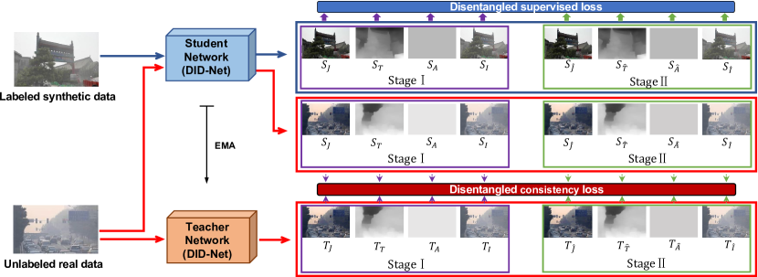
Figure 1. The schematic illustration of the developed DMT-Net. We first develop a disentangled image dehazing network (DID-Net; see Figure 2) for detecting haze-free maps, transmission maps, and atmospheric maps via a coarse-to-fine strategy, and build reconstructed haze maps. After that, we compute a supervised loss for labeled data and a consistency loss for unlabeled data and add them together to train our image dehazing netowrk. EMA: exponential moving average.

2.1. Traditional Dehazing Methods

Traditional dehazing methods utilized image priors (e.g., dark channel prior (He et al., 2011), color-line priors (Fattal, 2014), and haze-line priors (Berman and Avidan, 2016)) from hazy and latent clean images to compute a transmission map for haze removal. Please refer to Zhang et al. (Zhang and Patel, 2018) for a comprehensive review. By assuming that a linear relationship exists in the minimum channel between the hazy image and the haze-free image, a single image dehazing method is proposed based on linear transformation (Wang et al., 2017). Note that these hand-crafted priors from human observations do not always hold in diverse real-world hazy photos. Hence, they tend to suffer from undesirable color distortions (Ren et al., 2018).

2.2. Deep Learning based Dehazing Methods

Early works formulated CNNs to estimate a transmission map for recovering the clean image via the physical model in Eq. (1). Ren et al. (Ren et al., 2016) employed a coarse-scale network to predict a holistic transmission map and then used a fine-scale network for a transmission map refinement. Cai et al. (Cai et al., 2016) computed a transmission map by developing a DehazeNet equipped with BReLU based feature extraction layers. However, inaccurate transmission map estimation hinders haze removal quality of these methods.

Later, CNN-based methods directly learned the latent clean image from a single hazy image in an end-to-end manner. Yang et al. (Yang and Sun, 2018) predicted a clean image by integrating the physical model and image prior into a CNN. Song et al. (Song et al., 2018) presented a novel ranking convolutional neural network for single image dehazing. Li et al. (Li et al., 2018b) embedded VGG-features (Simonyan and Zisserman, 2015) and an $L_{1}$-regularized gradient prior into conditional generative adversarial network (cGAN) (Isola et al., 2017) for a clean image estimation. Ren et al. (Ren et al., 2018) learned confidence maps via an encoder-decoder network from three derived inputs and fused confidence maps for generating a final dehazed result. Zheng et al. (Zheng et al., 2021) devised a multi-guide bilateral learning for reaching a real-time dehazing of 4K images. However, the disjoint optimization on these deep models failed to capture the inherent relations among the transmission map, the atmospheric light, and the dehazed result, thereby degrading the overall dehazing performance.

To alleviate this issue, Zhang et al. (Zhang and Patel, 2018) employed two networks to estimate the transmission map and the atmospheric light separately, and computed the haze-free image according to the physical haze model (see Eq. (1)), which are all integrated into an end-to-end dehazing network (DCPDN). Deng et al. (Deng et al., 2019) attentively fused multiple mathematical haze separation models for image dehazing. Qu et al. (Qu et al., 2019) presented a dehazing GAN with a multi-resolution generator module, the enhancer module, and a multi-scale discriminator module. Liu et al. (Liu et al., 2019) devised a CNN with a pre-processing module, an attention-based multi-scale backbone module and a post-processing module. Deng et al. (Deng et al., 2020) stacked haze-aware representation distillation (HARD) modules with normalization layers into a GAN to attentively fuse global atmospheric brightness and local spatial structures. Dong et al. (Dong and Pan, 2020) explicitly utilized the physical model into a encoder-decoder network. Although improving the overall scene visibility, these methods are trained on synthesized images in a supervised learning manner, suffering from limited capability to generalize well to real-world hazy images.

Shao et al. (Shao et al., 2020) formulated a domain adaptation network with two image translation modules between synthesized and real hazy images and two image dehazing modules to alleviate the domain shift problem. However, the image dehazing modules of Shao et al. (Shao et al., 2020) learned CNN features from input hazy image to predict only one factor (i.e., the latent haze-free image), thereby hindering the dehazing performance. Although Li et al. (Li et al., 2020a) also leveraged the layer separation mechanism based on the physical model, this work mainly addressed the image dehazing in an unsupervised and zero-shot manner. To alleviate this issue, we develop a disentangled image dehazing network to learn disentangled feature presentations and leverage unlabeled data for improving dehazing performance.

3. Our Approach

Figure 1 shows the architecture of our DMT-Net, which learns disentangled representations and leverages unlabeled real-world hazy images for image dehazing. Specifically, we first develop a disentangled image dehazing network (DID-Net) to disentangle features at each scale into three components for jointly computing a dehazed map, a transmission map, and an atmospheric map via a coarse-to-fine mechanism (see predictions at Stage I and Stage II in Figure 1). Moreover, DID-Net reconstructs hazy images from the estimated maps of the three components, and then computes two reconstruction losses between the input hazy image and two reconstructed ones to make them similar. Then, our DID-Net is assigned to both the student network and the teacher network. During the training, the labeled data is fed into the student network, and a supervised loss is computed by adding prediction losses of three component maps and the reconstruction losses. Then, for unlabeled data, we produce one auxiliary image from the input hazy image and feed it into the student network and the teacher network, respectively. A disentangled consistency loss is computed on the two groups of three component maps and a reconstructed hazy map. In the testing procedure, we only utilize the student network to generate the dehazing result of an input image.

3.1. Disentangled Image Dehazing Network

According to the physical model of a haze process (see Eq. (1)), CNN features learned from an input hazy image encode information of three haze components, i.e. the haze-free map, the transmission map, and the atmospheric map. In this work, we propose a disentangled image dehazing network (DID-Net) by harnessing a disentangled feature learning strategy (Liu et al., 2018) to separate each feature into three components: a latent-distilled feature for predicting the haze-free map $J$, a transmission-distilled feature for predicting the transmission $T$, and a light-distilled feature for predicting the atmospheric-light map $A$, respectively; see Figure 2. By doing so, the proposed DID-Net is capable of simultaneously extracting features for all the three components, and hence providing comprehensive information for dehazing. Note that, before our work, two recently published papers (Zhang and Patel, 2018; Dong and Pan, 2020) also propose to jointly estimate the three components, but they utilize different networks for component estimation and totally rely on synthesized data, resulting in performance degradation on real-world photos.

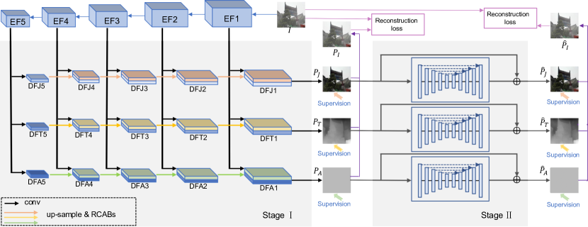
Figure 2. The schematic illustration of our DID-Net. Given an input hazy image $I$, we first extract a set of feature maps with different spatial resolutions, and then disentangle these features into three components: dehazing-distilled features for estimating a haze-free image ($J$), transmission-distilled features for estimating a transmission map ($T$), and light-distilled features for estimating an atmospheric light map ($A$). We then devise a coarse-to-fine strategy to predict $J$, $T$, and $A$. The coarse predictions ($P_{J}$, $P_{T}$, and $P_{A}$) are obtained via iteratively merging disentangled features, while refinement predictions ($\hat{P}_{J}$, $\hat{P}_{T}$, and $\hat{P}_{A}$) are produced by feeding coarse results into U-Net structures. Moreover, we reconstruct two hazy images ($P_{I}$ and $\hat{P}_{I}$) from the physical haze model with coarse/refined predictions, and compute reconstruction losses against the input hazy image $I$.

Figure 2 shows the schematic illustration of the proposed DID-Net. Specifically, given an input hazy image $I$, we first extract a set of feature maps with different spatial resolutions, and these feature maps are denoted as $\textit{EF}_{i}$ $(1\leq i\leq 5)$. We decompose each into latent-distilled disentangled features $\textit{DFJ}_{i}$, transmission-distilled disentangled features $\textit{DFT}_{i}$, and light-distilled disentangled features $\textit{DFA}_{i}$. After that, we devise a coarse-to-fine mechanism to estimate $J$, $T$, and $A$ based on these disentangled features. To do so, we first integrate disentangled features at different scales to generate coarse predictions for the three components (denoted as $P_{J}$, $P_{T}$ and $P_{A}$). Then, a hazy image $P_{I}$ can be figured out as follows:

(2) $$P_{I}(z)=P_{J}(z)\cdot P_{T}(z)+P_{A}(z)\cdot(1-P_{T}(z))\,$$

where $z$ is the $z$-th pixel.

We then feed the three coarse predictions, $P_{J}$, $P_{T}$ and $P_{A}$, into three independent U-Net based residual blocks to generate three corresponding refined predictions. The three refined predictions are denoted as $\hat{P}_{J}$, $\hat{P}_{T}$, and $\hat{P}_{A}$, respectively, based on which another hazy image $\hat{P}_{I}$ is computed from $\hat{P}_{J}$, $\hat{P}_{T}$, and $\hat{P}_{A}$:

(3) $$\hat{P}_{I}(z)=\hat{P}_{J}(z)\cdot\hat{P}_{T}(z)+\hat{P}_{A}(z)\cdot(1-\hat{P}_{T}(z))\ .$$

Once reconstructing two hazy images $P_{I}$ and $\hat{P}_{I}$ from the coarse and refined predictions, our DID-Net computes a reconstruction loss ($\mathcal{L}_{rec}$) between the input image $I$ and $P_{I}$ and $\hat{P}_{I}$. The $\mathcal{L}_{rec}$ is defined as:

(4) $$\mathcal{L}_{rec}=|I-P_{I}|_{L_{1}}+|I-\hat{P}_{I}|_{L_{1}}\ ,$$

where $|\cdot|_{L_{1}}$ is the $L_{1}$ loss function.

How to generate coarse predictions.  As shown in Figure 2, our DID-Net devises three independent branches to progressively aggregate disentangled features from deep layers to shallow layers for generating coarse predictions $P_{J}$, $P_{T}$, and $P_{A}$. Here, we take the branch for generating the haze-free image prediction as an example to describe the workflow. This branch aggregates $\textit{DFJ}_{i}$ $(1\leq i\leq 5)$ for predicting the haze-free prediction, where the key operation is to merge features at adjacent layers. When fusing two adjacent features ($\textit{DFJ}_{i}$ and $\textit{DFJ}_{i-1}$, $2\leq i\leq 5$), we up-sample the low-resolution feature ${\textit{DFJ}}_{i}$ to the same spatial resolution with the high-resolution feature $\textit{DFJ}_{i-1}$, enhance upsampled features by feeding them into a series of residual channel attention blocks (RCABs) (Zhang et al., 2018), and apply a $1$$\times$$1$ convolutional layer on the concatenation of the RCAB-enhanced feature and the high-resolution feature $\textit{DFJ}_{i-1}$ to output a merged feature map, which is denoted as $H_{i-1}$. The $H_{i-1}$ can be computed by:

(5) $$H_{i-1} =\mathcal{M}(\textit{DFJ}_{i},\textit{DFJ}_{i-1})$$

$$=conv(concate(\Phi_{\textit{RCAB}}(\textit{DFJ}_{i}),\textit{DFJ}_{i-1}))\ ,$$

where $\mathcal{M}(\cdot)$ denotes the operation of merging two features; the $conv$ is a $1$$\times$$1$ convolutional layer; the $\Phi_{\textit{RCAB}}$ is the refinement block consisting of a number of RCABs. Then, similarly, we merge $H_{i-1}$ with features DFJ at the next CNN layer until reaching features DFJ (with the largest spatial resolution) at the first CNN layer, and finally pass the resultant features to a $1$$\times$$1$ convolutional layer for predicting $P_{J}$:

(6) $$P_{J} =conv(\mathcal{M}(\textit{DFJ}_{1},H_{2}))\ ,$$

$$H_{2} =\mathcal{M}(\textit{DFJ}_{2},H_{3})\ ,$$

$$H_{3} =\mathcal{M}(\textit{DFJ}_{3},H_{4})\ ,$$

$$H_{4} =\mathcal{M}(\textit{DFJ}_{4},\textit{DFJ}_{5})\ ,$$

where $\mathcal{M}$ is the feature operation of Eq. (5). We conduct the similar operations to incrementaly aggregate transmission-distilled features and light-distilled features. Note that the numbers of RCABs in merging features are different. In our experiments, we empirically use $20$ RCABs to merge adjacent features for computing $P_{J}$ and $P_{T}$, and $2$ RCABs to merge features for computing $P_{A}$, since $P_{A}$ is a global parameter and simpler than the other two components.

How to generate fine predictions. We further pass these coarse predictions, $P_{J}$, $P_{T}$, and $P_{A}$, to a U-Net residual block to produce their refined results. For example, given the coarse haze-free map prediction $P_{J}$, we pass it to a U-Net (Ronneberger et al., 2015) with $5$ convolutional layers, to produce an intermediate image $\mathcal{U}(P_{J})$, which is then added with $P_{J}$ to obtain a refinement (denoted as $\hat{P}_{J}$) of $P_{J}$,

(7) $$\hat{P}_{J}=P_{J}+\mathcal{U}(P_{J})\ .$$

Similarly, we compute a refinement $\hat{P}_{T}$ of $P_{T}$, and a refinement $\hat{P}_{A}$ of $P_{A}$ as follows:

(8) $$\hat{P}_{T} =P_{T}+\mathcal{U}(P_{T})\ ,$$

$$\hat{P}_{A} =P_{A}+\mathcal{U}(P_{A})\ ,$$

where $\mathcal{U}(P_{T})$ and $\mathcal{U}(P_{T})$ are the U-Net structure on $P_{T}$ and $T_{A}$. Note that $\mathcal{U}(P_{J})$, $\mathcal{U}(P_{T})$, and $\mathcal{U}(P_{A})$ have the same encoder-decoder structures, but do not share network parameters.

3.2. Supervised Loss on Labeled data

Note that a synthesized hazy image (labeled image) is usually generated by passing a given clean image, a given transmission image, and a given atmospheric image to the physically-based model introduced by Eq. (1), which can be naturally taken as the ground truths. Based on the ground truths, we first compute a disentangled multi-task supervised loss (denoted as $\mathcal{L}_{dst}(x)$) for a labeled hazy image ($x$) by adding the supervised losses of the clean image prediction ($\mathcal{L}^{s}_{J}$), transmission image prediction ($\mathcal{L}^{s}_{T}$), and atmospheric image prediction ($\mathcal{L}^{s}_{A}$), i.e.

(9) $$\mathcal{L}_{dst}(x)=\mathcal{L}^{s}_{J}+\alpha_{1}\mathcal{L}^{s}_{T}+\alpha_{2}\mathcal{L}^{s}_{A}\ ,$$

where

(10) $$\mathcal{L}^{s}_{J}=|G_{J}-P_{J}|_{L_{1}}+|G_{J}-\hat{P}_{J}|_{L_{1}}\ ,$$

$$\mathcal{L}^{s}_{T}=|G_{T}-P_{T}|_{L_{1}}+|G_{T}-\hat{P}_{T}|_{L_{1}}\ ,$$

$$\mathcal{L}^{s}_{A}=|G_{A}-P_{A}|_{L_{1}}+|G_{A}-\hat{P}_{A}|_{L_{1}}\ .$$

Here, $G_{J}$, $G_{T}$ and $G_{A}$ represent the ground truths of the clean image, the transmission image and the atmospheric image, respectively. We empirically set the weights $\alpha_{1}$$=$$0.3$ and $\alpha_{2}$$=$$0.1$ in the network training. By adding $\mathcal{L}_{dst}$ with the reconstruction loss of Eq. (4), we compute the supervised loss of labeled data as follows:

(11) $$\mathcal{L}^{s}(x)=\mathcal{L}_{dst}(x)+\alpha_{3}\mathcal{L}_{rec}\ ,$$

where $\alpha_{3}$$=$$0.1$ in our experiment.

3.3. Consistency Loss on Unlabeled Data

For the unlabeled real-world data, we pass it into the student network to obtain eight results, which are two clean images (denoted as $S_{J}$ and $S_{\hat{J}}$), two transmission images ($S_{T}$ and $S_{\hat{T}}$), and two atmospheric images ($S_{A}$ and $S_{\hat{A}}$), and two reconstructed hazy images ($S_{I}$ and $S_{\hat{I}}$). Meanwhile, by first adding a Gaussian noise into the real-world hazy image and feeding the noisy image into the teacher network, we can generate another two clean images ($T_{J}$ and $T_{\hat{J}}$), two transmission images ($T_{T}$ and $T_{\hat{T}}$), two atmospheric images ($T_{A}$ and $T_{\hat{A}}$), and two reconstructed hazy images ($T_{I}$ and $T_{\hat{I}}$). We then enforce the predictions of eight prediction results from the student network and the teacher network to be consistent, resulting in a disentangled multi-task consistency loss ($\mathcal{L}^{c}$). Mathematically, $\mathcal{L}^{c}$ for an unlabeled image (denoted as $y$) is

(12) $$\mathcal{L}^{c}(y)=\mathcal{L}^{c}_{J}+\alpha_{4}\mathcal{L}^{c}_{T}+\alpha_{5}\mathcal{L}^{c}_{A}+\alpha_{6}\mathcal{L}^{c}_{rec}\ ,$$

where

(13) $$\mathcal{L}^{c}_{J}=|S_{J}-T_{J}|_{L_{1}}+|S_{\hat{J}}-T_{\hat{J}}|_{L_{1}}\ ,$$

$$\mathcal{L}^{c}_{T}=|S_{T}-T_{T}|_{L_{1}}+|S_{\hat{T}}-T_{\hat{T}}|_{L_{1}}\ ,$$

$$\mathcal{L}^{c}_{A}=|S_{A}-T_{A}|_{L_{1}}+|S_{\hat{A}}-T_{\hat{A}}|_{L_{1}}\ ,$$

$$\mathcal{L}^{c}_{rec}=|S_{I}-T_{I}|_{L_{1}}+|S_{\hat{I}}-T_{\hat{I}}|_{L_{1}}\ ,$$

$\mathcal{L}^{c}_{J}$, $\mathcal{L}^{c}_{T}$, $\mathcal{L}^{c}_{A}$, and $\mathcal{L}^{c}_{rec}$ denote the consistency loss of the clean image estimation, the transmission image estimation, the atmospheric image estimation, and the reconstructed hazy image, respectively. For simplicity, we set $\alpha_{4}=\alpha_{1}=0.3$, $\alpha_{5}=\alpha_{2}=0.1$, and $\alpha_{6}=\alpha_{3}=$$0.1$.

3.4. Our Network

As a semi-supervised framework, our method fuses labeled synthesized images and unlabeled real-world images for training. The total loss of our network is

(14) $$\mathcal{L}_{total}=\sum_{x\in\mathbb{L}}\mathcal{L}^{s}(x)+\mu\sum_{y\in\mathbb{U}}\mathcal{L}^{c}(y)\ ,$$

where $\mathbb{L}$ and $\mathbb{U}$ denote the labeled dataset and the unlabeled dataset. $\mathcal{L}^{s}(x)$ represents the supervised loss (see Eq. (11)) for a labeled hazy image x of $\mathbb{L}$. $\mathcal{L}^{c}(y)$ is the consistency loss (see Eq. (12)) for a unlabeled hazy image of $\mathbb{U}$. We follow (Chen et al., 2020) to apply a time dependent Gaussian warming up function to compute the weight $\mu$: $\mu(t)=\mu_{max}e^{(-5{(1-t/t_{max})}^{2})}$, where $t$ denotes the current training iteration and $t_{max}$ is the maximum training iteration. In our experiments, we empirically set $\mu_{max}$$=$$1$. We minimize $\mathcal{L}_{total}$ to train the student network, and the parameters of the teacher network are updated via the exponential moving average (EMA) strategy with a EMA deay of $0.99$; please refer to  (Laine and Aila, 2016; Tarvainen and Valpola, 2017; Chen et al., 2020) for details.

3.5. Our unlabeled data

Note that (Shao et al., 2020) provides an unlabeled dataset with $1,000$ real-world hazy images to train a domain adaption network for haze removal. To conduct fair comparisons, we use the same real-world dataset of (Shao et al., 2020) as the unlabeled data of our network.

3.6. Training and Testing Strategies

Training parameters. To accelerate the training procedure and reduce the overfitting risk, we initialize the parameters of DID-Net (student network) by ResNeXt (Xie et al., 2017), which has been well-trained for the image classification task on the ImageNet. Other parameters in the DID-Net are initialized as random values. We implement our framework in PyTorch and utilize ADAM optimizer to train the network. The learning rate is adjusted by a poly strategy (Liu et al., 2016) with the initial learning rate of $0.0001$ and the power of $0.9$. We randomly crop all the labeled and unlabeled images to $240$$\times$$240$ for the training on two GTX 2080Ti GPU, and augment the training set by random horizontal flipping. We use the mini-batch size of $16$, which means the usage of $8$ labeled images and $8$ unlabeled data images in each training epoch.

Inference.  In the testing stage, we feed the input image into the student network and utilize the predicted dehazed map of the student network as the final output of our network.

4. Experimental Results

Table 1. Quantitative comparisons between our network and compared methods on three synthetic dehazing datasets.

		Haze4K		SOTS (Ren et al., 2018)		HazeRD (Zhang et al., 2017)
method	Year	PSNR	SSIM	PSNR	SSIM	PSNR	SSIM
Our DMT-Net	-	28.53	0.96	29.42	0.97	18.55	0.85
Our DID-Net	-	27.81	0.95	28.30	0.95	18.07	0.84
DA (Shao et al., 2020)	2020	24.03	0.90	27.76	0.93	18.07	0.63
FFA-Net (Qin et al., 2020)	2020	26.97	0.95	26.88	0.95	17.56	0.80
MSBDN (Hang et al., 2020)	2020	22.99	0.85	24.15	0.86	16.87	0.75
DM2F-Net (Deng et al., 2019)	2019	24.61	0.92	23.87	0.91	15.88	0.74
GDN (Liu et al., 2019)	2019	23.29	0.93	26.05	0.95	15.92	0.77
EPDN (Qu et al., 2019)	2019	21.08	0.86	23.82	0.89	17.37	0.56
DCPDN (Zhang and Patel, 2018)	2018	23.86	0.91	19.39	0.65	16.12	0.34
GFN (Ren et al., 2018)	2018	-	-	22.30	0.88	13.98	0.37
AOD-Net (Li et al., 2017)	2017	17.15	0.83	19.06	0.85	15.63	0.45
DehazeNet (Cai et al., 2016)	2016	19.12	0.84	21.14	0.85	15.54	0.41
MSCNN (Ren et al., 2016)	2016	14.01	0.51	17.57	0.81	15.57	0.42
NLD (Berman and Avidan, 2016)	2016	15.27	0.67	17.27	0.75	16.16	0.58
DCP (He et al., 2011)	2011	14.01	0.76	15.49	0.64	14.01	0.39

PSNR / SSIM	21.80 / 0.70	24.63 / 0.94	21.99/0.92	22.70 / 0.86	22.17 / 0.87	27.87 / 0.95	28.63 / 0.97	$\infty$ / 1
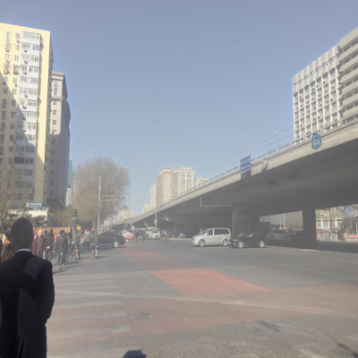
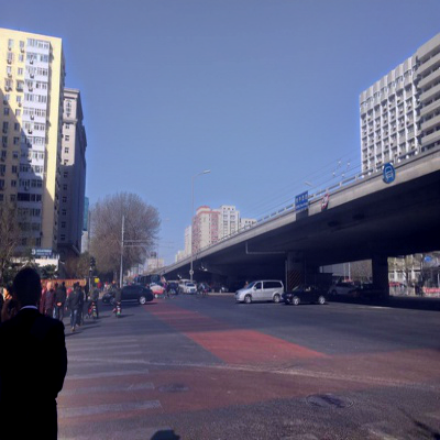
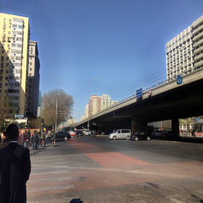
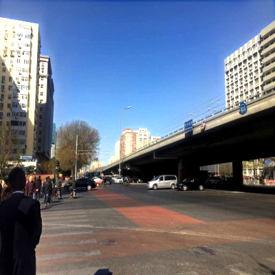
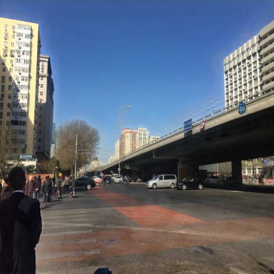
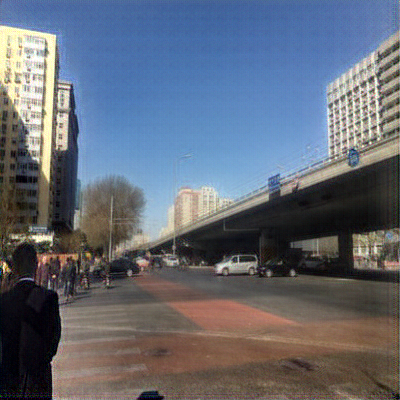
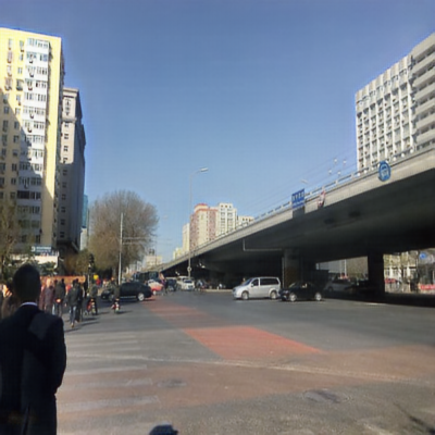
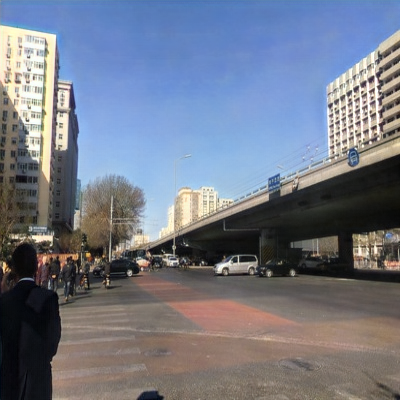
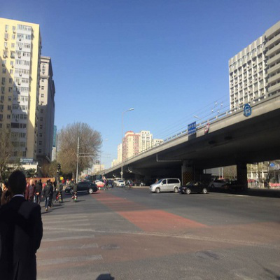
PSNR / SSIM	17.76 / 0.83	22.92 / 0.96	20.29/ 0.86	22.34 / 0.94	18.92 / 0.84	24.99 / 0.93	27.69 / 0.96	$\infty$ / 1
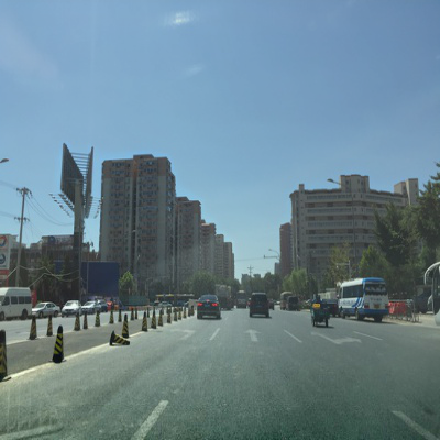
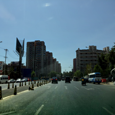
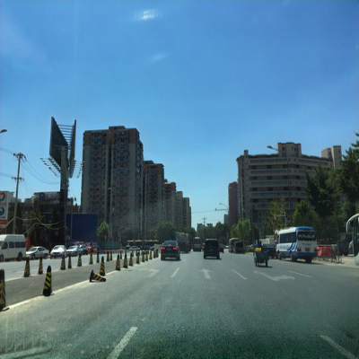
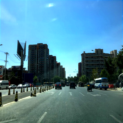
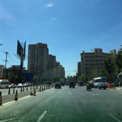
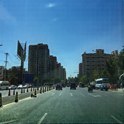
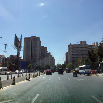
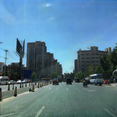
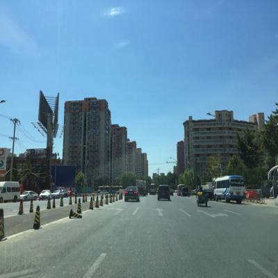
PSNR / SSIM	10.64 / 0.72	18.99 / 0.91	18.63/ 0.94	21.67 / 0.95	17.72 / 0.83	17.03 / 0.86	27.14 / 0.96	$\infty$ / 1
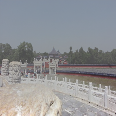
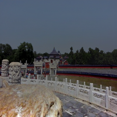
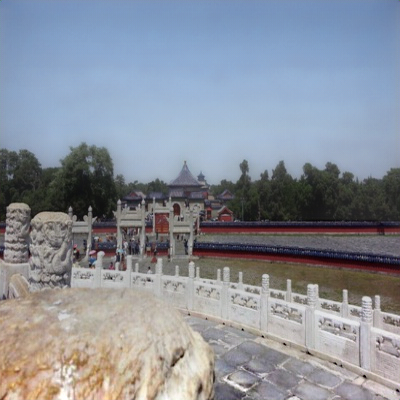
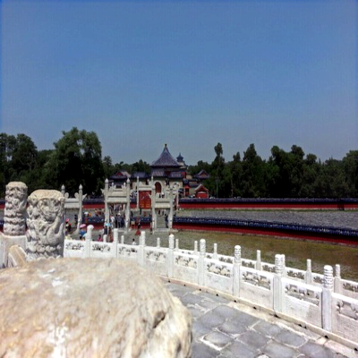
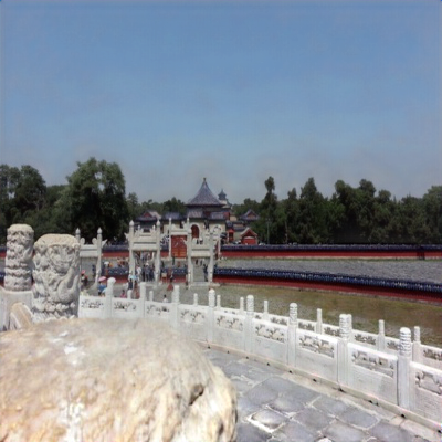
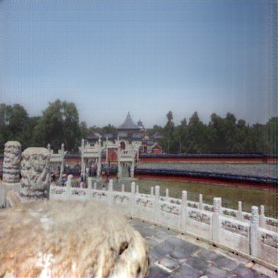
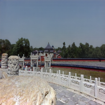
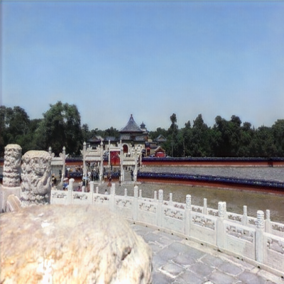
(a) Input Image	(b) DehazeNet	(c) GDN	(d) DM2F-Net	(e) FFA-Net	(f) MSBDN	(g) DA	(h) Our Method	(i) Ground truth

Figure 3. Visual comparisons on dehazed results of various methods on synthetic hazy photos. Please zoom in for a better illustration.

We compare our dehazing network against 13 state-of-the-art image dehazing methods, including DCP (He et al., 2011), NLD (Berman and Avidan, 2016), MSCNN (Ren et al., 2016), DehazeNet (Cai et al., 2016), AOD-Net (Li et al., 2017), GFN (Ren et al., 2018), DCPDN (Zhang and Patel, 2018), EPDN (Qu et al., 2019), GDN (Liu et al., 2019), DM²F-Net (Deng et al., 2019), FFA  (Qin et al., 2020), MSBDN (Hang et al., 2020) and DA (Shao et al., 2020). Among the compared methods, DCP and NLD focused on hand-crafted features for haze removal, while others are based on convolutional neural networks (CNNs). We retrain the original (released) implementations of these methods or directly report their results on the public datasets. Furthermore, we employ two widely-used metrics for quantitative comparisons, and they are peak signal to noise ratio (PSNR) (Zhu et al., 2017a, 2021) and structural similarity index (SSIM) (Wang et al., 2004; Zhu et al., 2017b).

Datasets.  We first test each image dehazing method on a public benchmark dataset, i.e., SOTS (Shao et al., 2020), which consists of 1,000 testing images. We follow existing works (Shao et al., 2020) to set the associate training set with 6,000 synthesized images, which consists of 3,000 from the indoor training set (ITS), and 3,000 from the outdoor training set (OTS) of the RESIDE dataset (Li et al., 2018c). Second, HazeRD (Zhang et al., 2017) containing $15$ outdoor images with more realistic haze is introduced for testing.

Apart from SOTS and HazeRD, we also create a synthesized dataset (denoted as Haze4K) with 4,000 hazy images, in which each hazy image has the associate ground truths of a latent clean image, a transmission map, and an atmospheric light map. To be specific, we collected 1,000 clean images by randomly selecting $500$ indoor images from NYU-Depth (Silberman et al., 2012) and $500$ outdoor images from OTS (Li et al., 2018c). Among them, $250$ images are randomly selected from both indoor image set ($125$ images) and outdoor image set ($125$ images), to form the test set, and the remaining $750$ images are used for the training set. After that, for each clean image, we followed (Zhang and Patel, 2018) to randomly sample four parameter settings, i.e. atmospheric light conditions $A\in[0.5,1]$ and scattering coefficients $\beta\in[0.5,2]$, to generate transmission maps and atmospheric light maps, which are then employed to obtain the corresponding hazy images via the physic model in Eq. (1). Hence, Haze4K has 4,000 hazy images with 3,000 training images and 1,000 testing images.

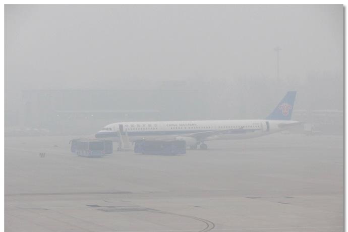
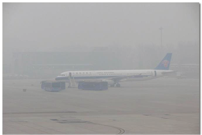
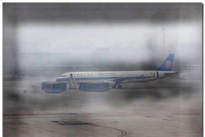
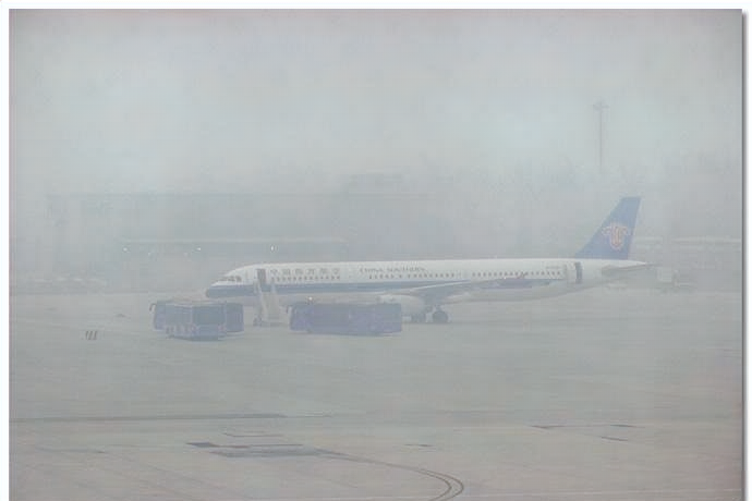
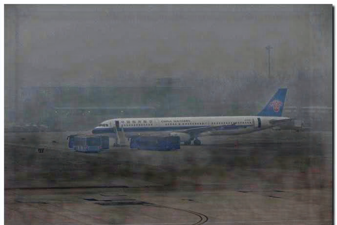
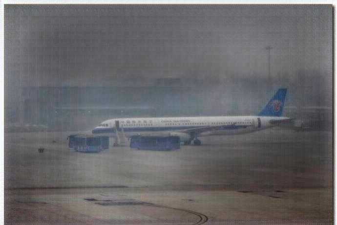
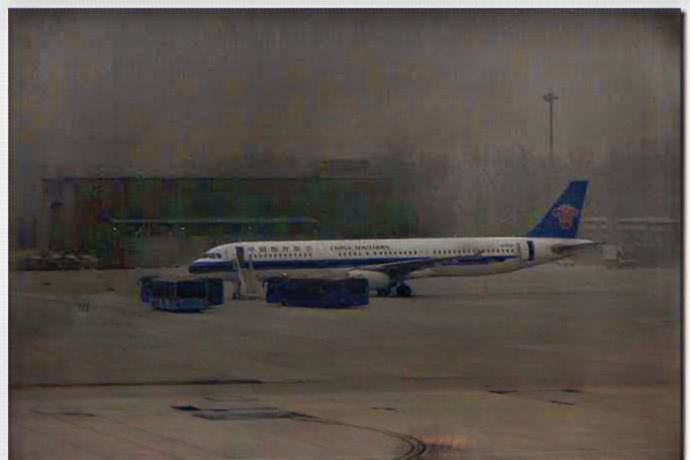
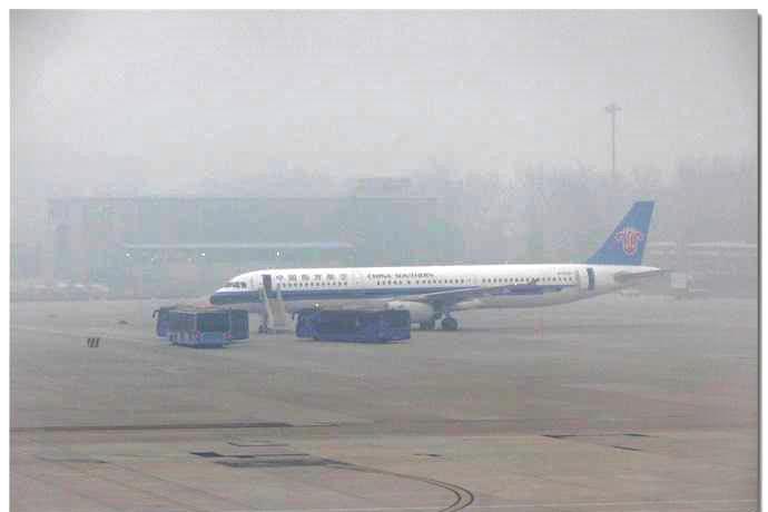
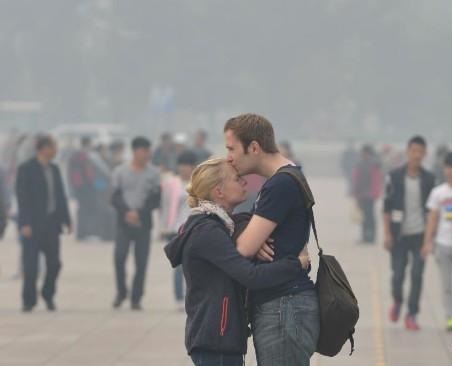
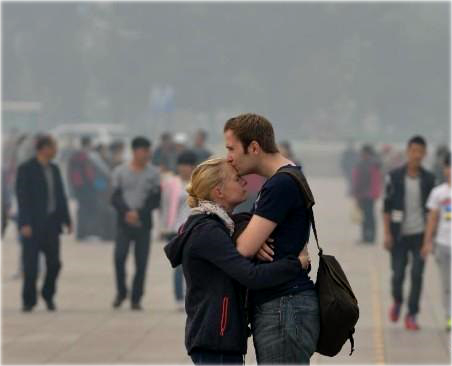
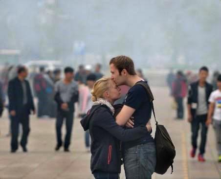
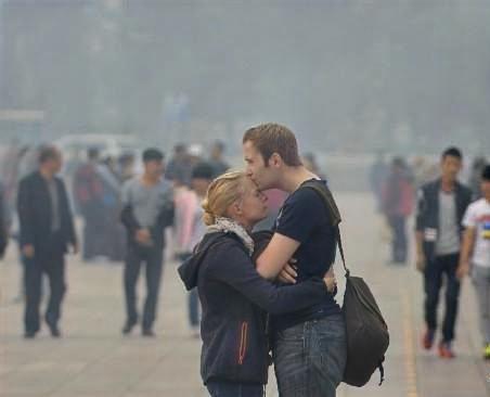
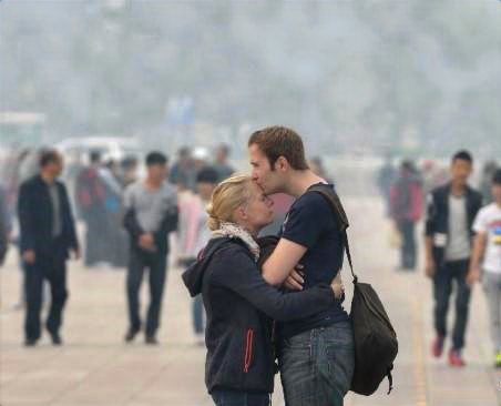
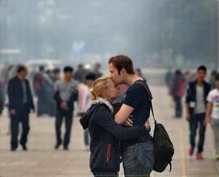
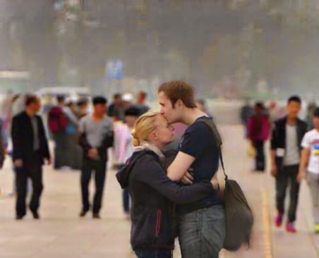
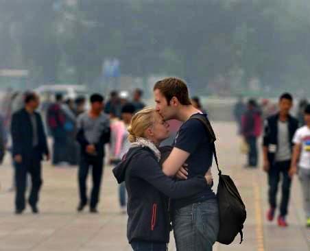
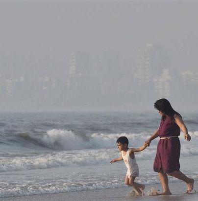
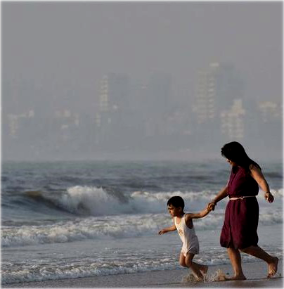
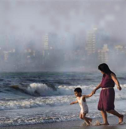
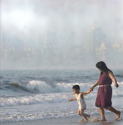
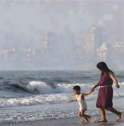
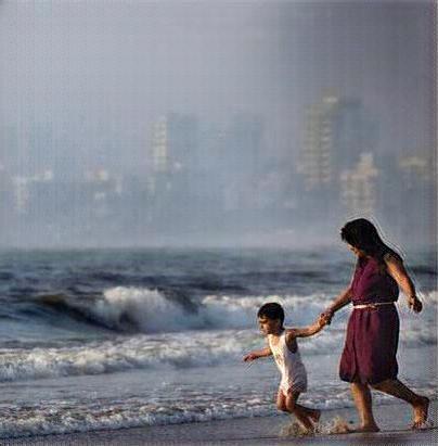
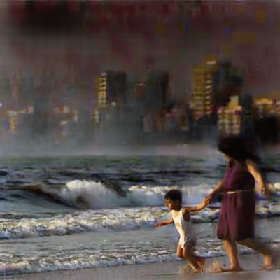
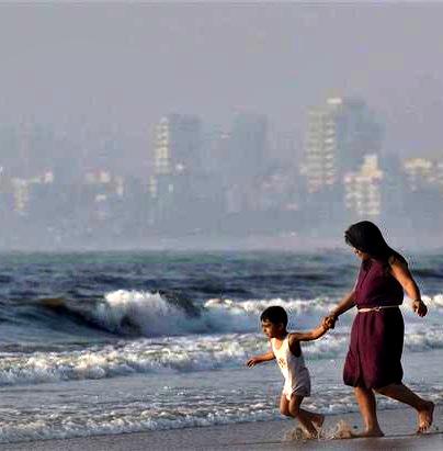
(a) Input Image	(b) AOD-Net	(c) GDN	(d) DM2F-Net	(e) FFA-Net	(f) MSBDN	(g) DA	(h) Our Method

Figure 4. Visual comparisons on dehazed results produced by our network (h) and SOTA methods (b)-(g) on real-world hazy photos (a).

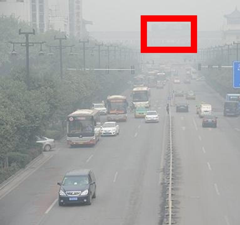
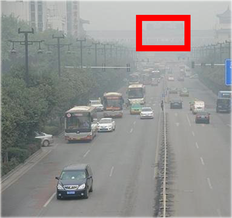
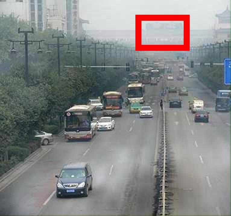
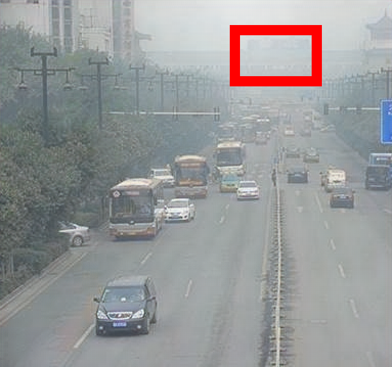
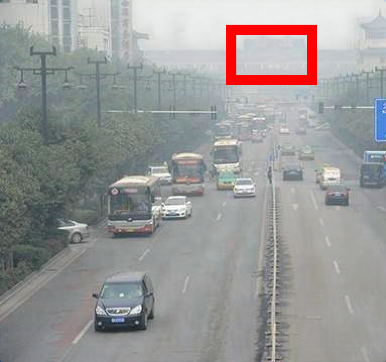
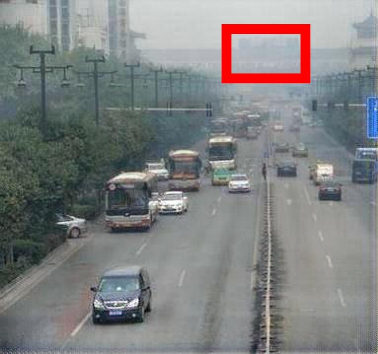
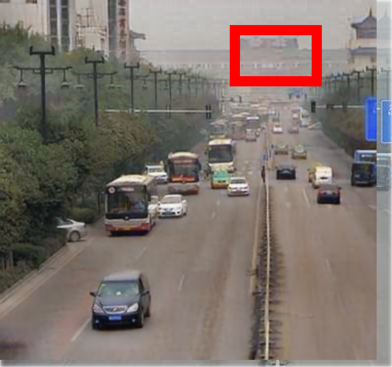
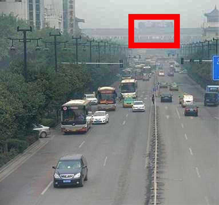
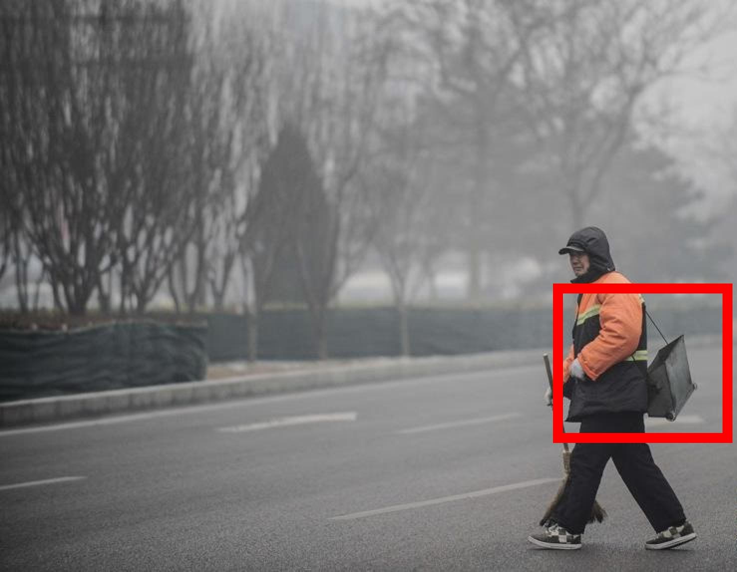
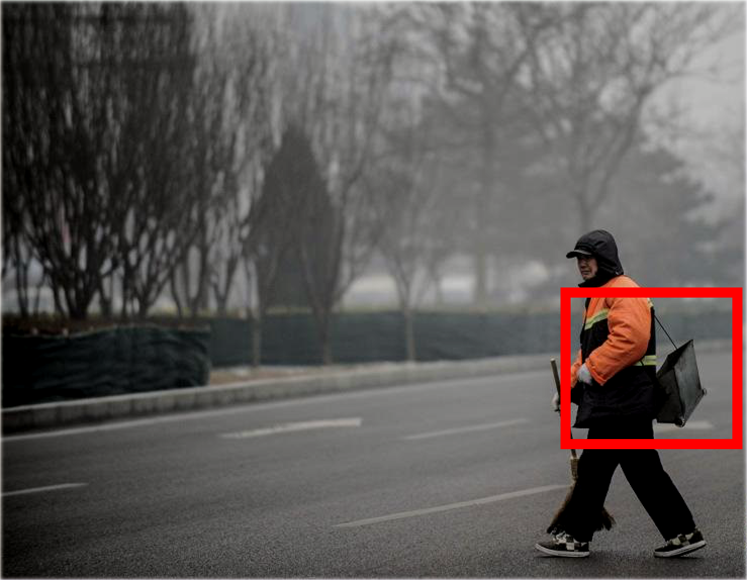
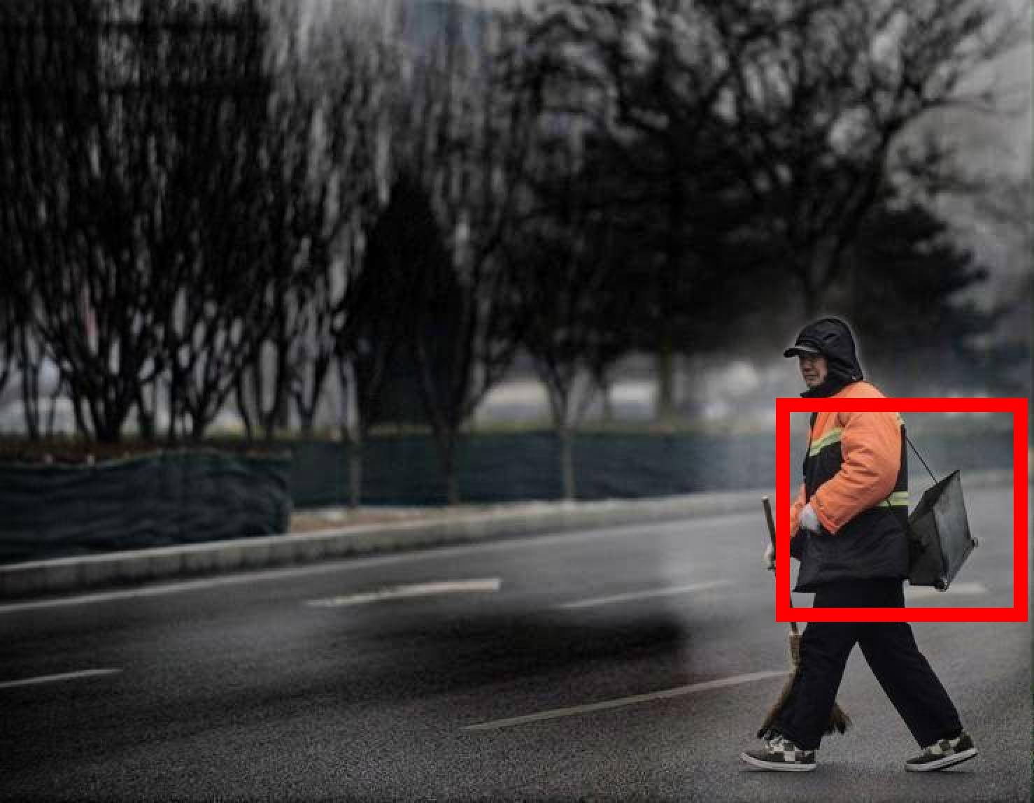
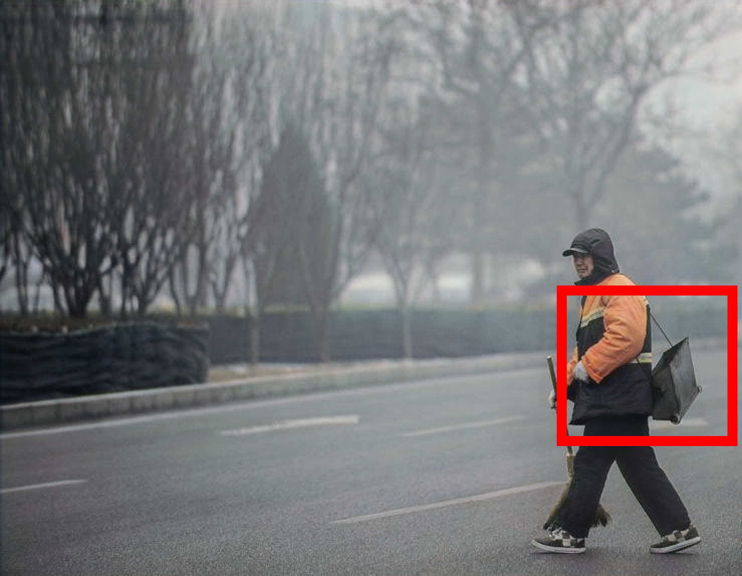
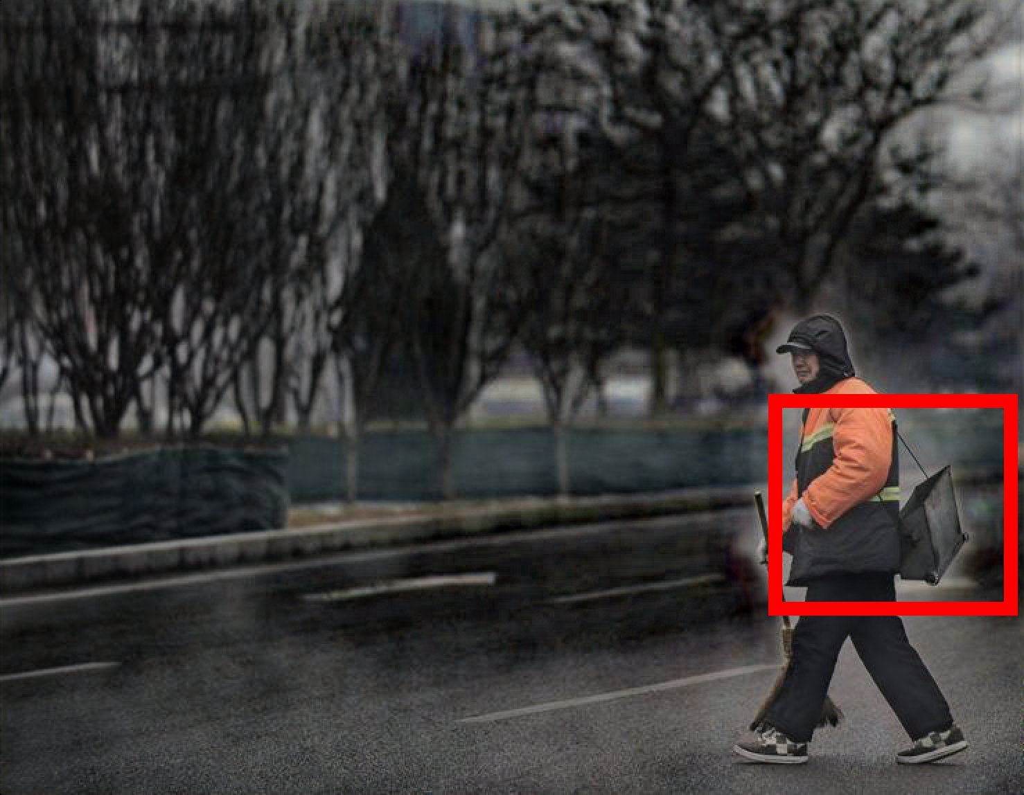
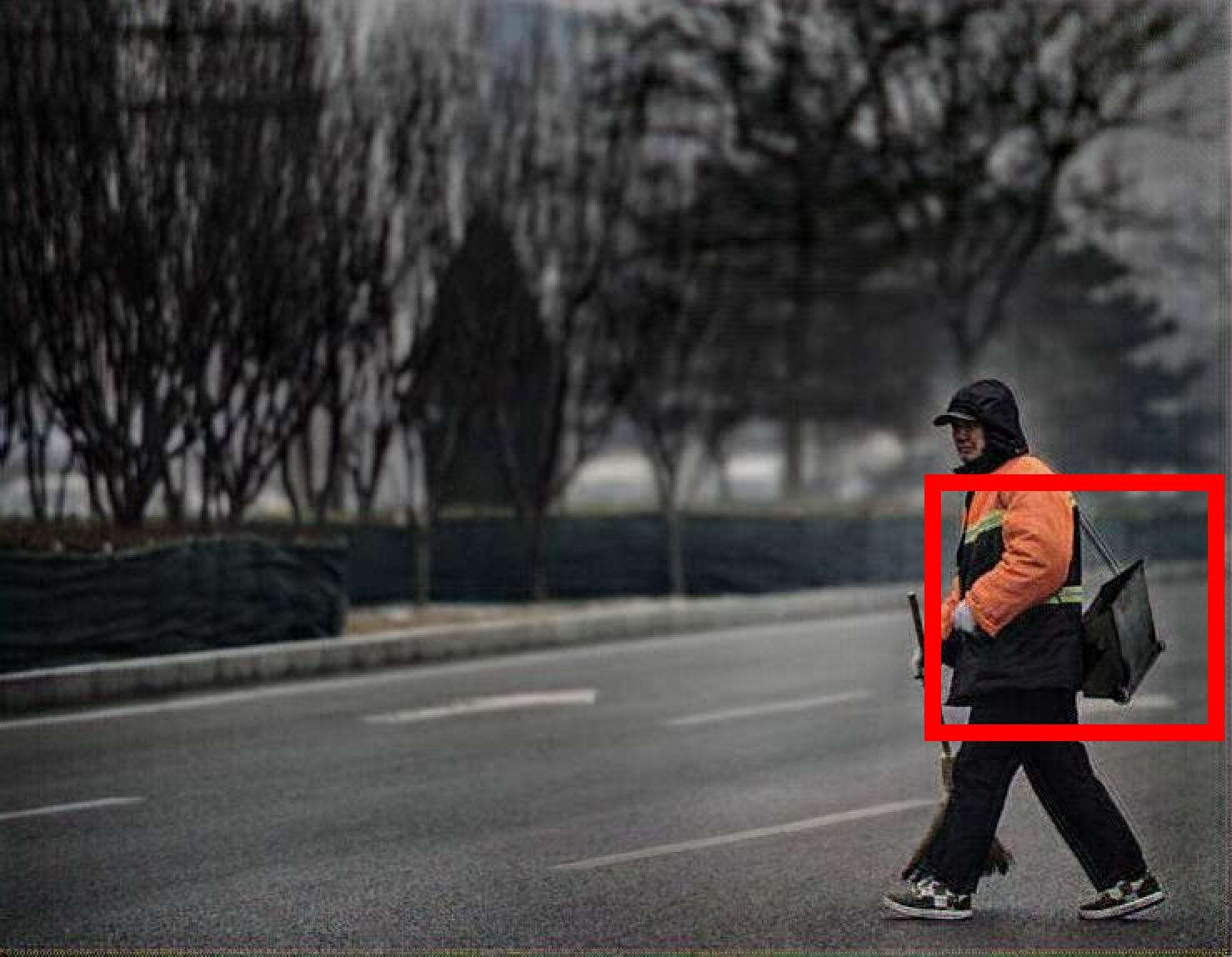
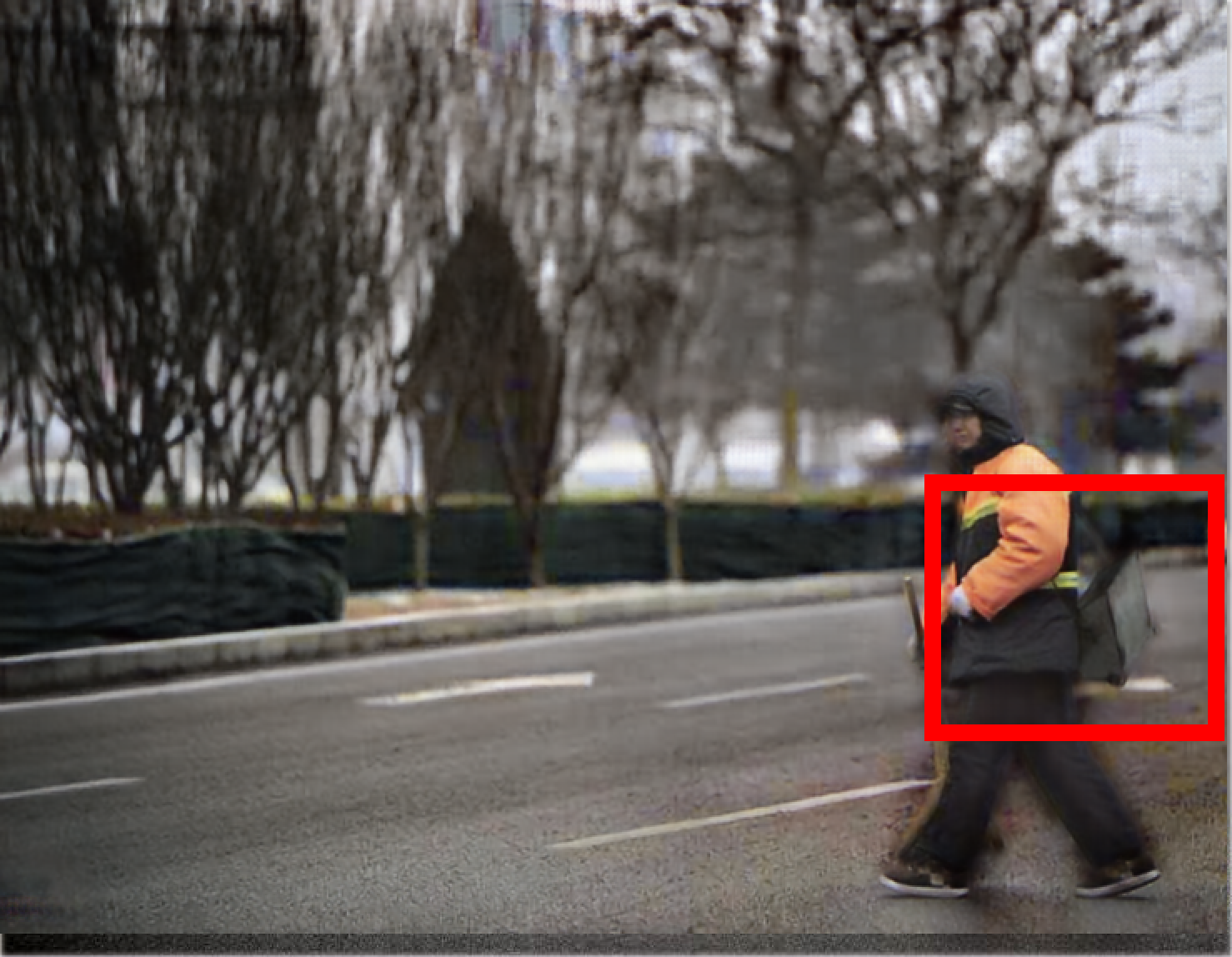
(a) Input Image	(b) AOD-Net	(c) GDN	(d) DM2F-Net	(e) FFA-Net	(f) MSBDN	(g) DA	(h) Our Method

Figure 5. Visual comparisons on dehazed results produced by our network (h) and SOTA methods (b)-(g) on more real-world hazy photos (a). Please see blown-up views for better visual comparisons.

4.1. Results on Synthetic Images

We retrain released models of these compared methods on the training set of our Haze4K dataset to obtain their results, while we follow the training setting of DA (Shao et al., 2020) to produce our results on SOTS and HazeRD for fair comparisons.

Table 1 reports PSNR and SSIM scores of different dehazing methods. In general, CNN-based methods have larger PNSR and SSIM values than hand-crafted-prior based methods (DCP & NLD). Among all the compared methods, FFA-Net has the largest PSNR and SSIM scores (i.e., 26.97 and 0.95) on Haze4K, and the largest SSIM score (0.80) on HazeRD, while DA has the largest PSNR and SSIM values (i.e., 27.76 and 0.93) on SOTS, and the largest SSIM value (18.07) on HazeRD. Also note that our Haze4K dataset contains more challenging dehazing photos than SOTA, and existing dehazing methods suffer from a degraded PSNR and SSIM performance. DID-Net, as our sub-network with only labeled data, already outperforms most existing CNN-based methods in terms of PSNR and SSIM metrics, which proves the effectiveness of our disentangled feature learning for haze removal. Furthermore, our method consistently has the largest PSNR and SSIM scores on Haze4K, SOTS, and HazeRD, demonstrating that our semi-supervised dehazing network can better recover the underlying clean images for these hazy images.

Figure 3 visually compares the dehazed results. In the first and third images, DehazeNet produces an obvious color distortion in the ground regions of the dehazed results. Although obtaining a better dehazing performance than DehazeNet, the CNN-based methods (e.g., GDN, DM²F-Net, FFA, and MSBDN) tend to darken several areas in their results; see Figures 3 (c)-(f). DA may produce color distortion especially in the sky regions for the three images. In contrast, the dehazed results of our network in Figure 3 (h) is closest to the latent ground truth images (see Figure 3 (i)). To summarize, our dehazed results (DMT-Net) tend to produce higher visual quality and less color distortions, which are also verified by the largest PSNR and SSIM values shown in Figure 3.

4.2. Results on Real-world Images

Figure 4 and Figure 5 visually compare the dehazed maps on real-world hazy photos from the RESIDE dataset (Li et al., 2018c). DA suffers from color distortions in almost all the five photos. This is particularly evident in the first and third images of Figure 4. GDN tends to darken several areas; see the first image (the lane area) of Figure 5. AOD-Net, DM²F-Net, FFA, and MSBDN remove few fog, and there is still a large amount of fog in the generated images; see blown-up views of Figure 5. Our method can more effectively remove haze while producing realistic colors than these compared state-of-the-art methods.

PSNR / SSIM	21.65 / 0.81	26.72 / 0.83	27.43/0.92	29.64 / 0.94	$\infty$ / 1
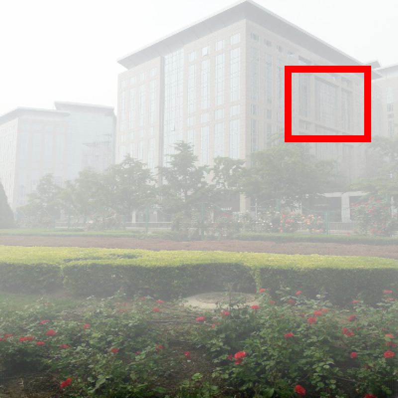
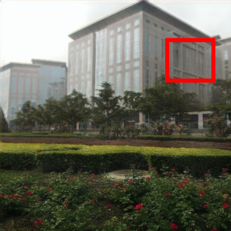
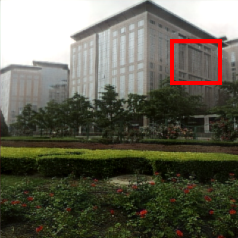
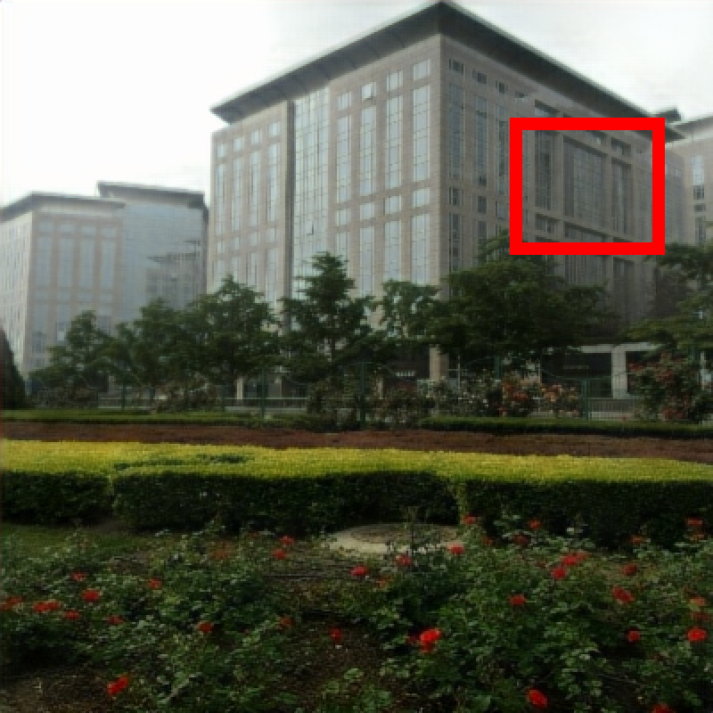
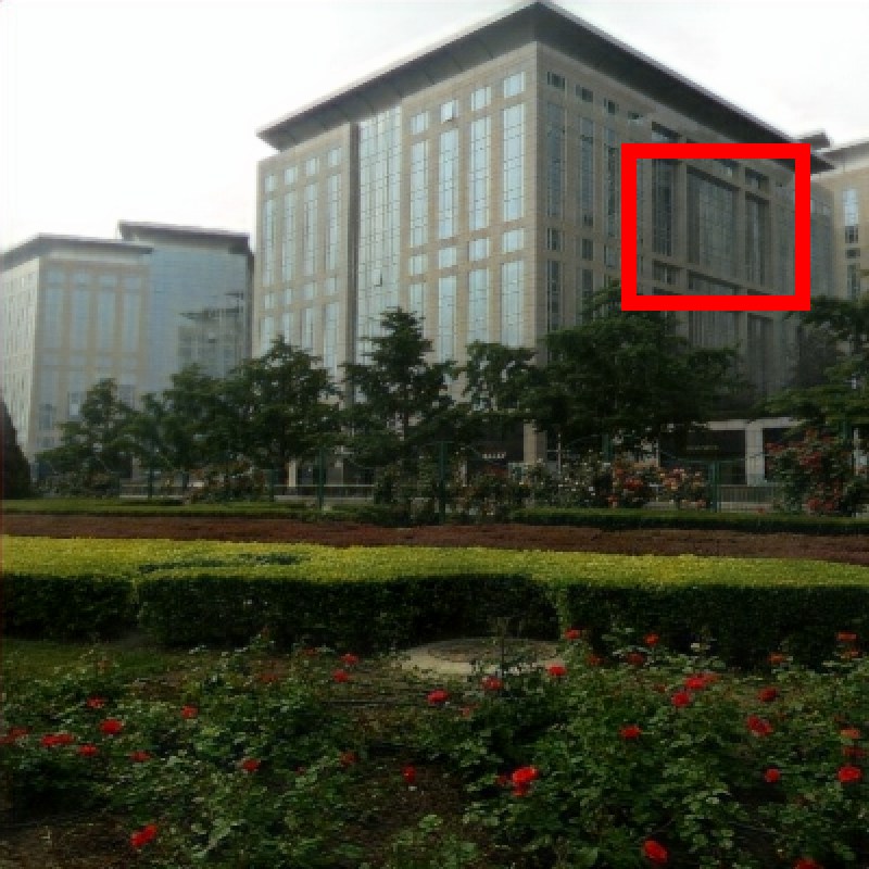
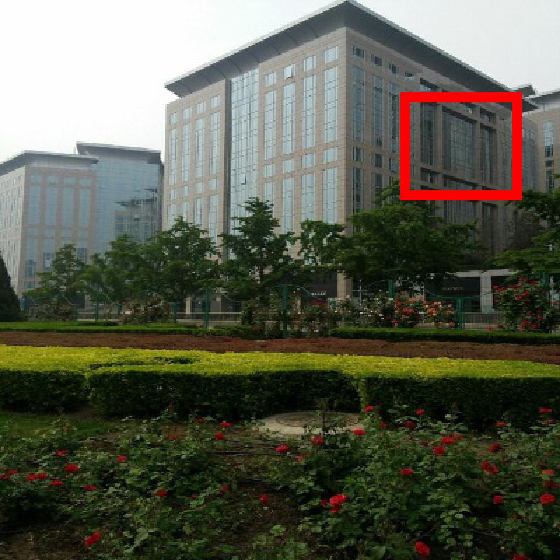
(a) Input Image	(b) basic	(c) basic+StageI	(d) baisc+two-stages	(e) Our method	(f) Ground truth

Figure 6. Visual comparisons of dehazed results produced by our method and three baselines (ablation study). Please zoom in for a better illustration.

Table 2. Average PSNR and SSIM values in ablation study.

	Haze4K		SOTS (Ren et al., 2018)
method	PSNR	SSIM	PSNR	SSIM
basic	25.39	0.93	27.09	0.94
basic+StageI	26.85	0.94	27.82	0.95
basic+two-stages	27.81	0.95	28.30	0.95
DMT-Net (ours)	28.53	0.96	29.42	0.97

4.3. Ablation Study

Baseline network setting.  We perform ablation study experiments to evaluate the effectiveness of major components of our network. Here, we construct three baseline networks, and list their PSRN and SSIM results on Haze4K and SOTS (Li et al., 2019; Ren et al., 2018). The first baseline (denoted as “basic”) is constructed by removing the two branches of predicting transmission maps and atmospheric maps, removing prediction refinement, and removing unlabeled data. It means that “basic” is equal to progressively merge ${EF}_{5}$ to ${EF}_{1}$ on labeled data for predicting a haze-free map $P_{J}$. The second baseline (denoted as “basic+StageI”) adds the feature disentangling operations into “basic”, demonstrating that three branches to fuse disentangled features are employed. Lastly, we construct the third baseline (denoted as “basic+two-stages”) by adding U-Net refinement blocks to coarse predictions, which equals to train DID-Net (see Fig. 2) on labeled data for haze removal.

Quantitative comparison.  Table 2 summarizes PSNR and SSIM results of our method (DMT-Net) and the constructed three baselines. From the results, we find that “basic+StageI” has larger PSNR and SSIM scores than “basic”, which indicates disentangling CNN features from the input hazy can produce a more accurate dehazed result. Similarly, “basic+two-stages” has a superior PSNR and SSIM performance than “basic+StageI”, showing that three refinement blocks further improve the dehazing performance. Lastly, our DMT-Net outperforms “basic+two-stages” in terms of PSNR and SSIM metrics. It further demonstrates that the unlabeled data helps our method to obtain better performance.

Visual comparison.  As shown in Figure 6, “basic+StageI” tends to produce a relatively clean texture than “basic”, but both of them tend to modify colors of the building regions. This phenomenon is improved by “basic+two-stages”, and our method can further generates better textures and visual quality. In conclusion, our network can effectively remove haze and simultaneously maintain the latent color distributions inside building regions, which is also proved by superior PSRN/SSIM scores.

4.4. More Discussions

Hyper-parameter study.   As presented in Eq. 9 and Eq. 12, our supervised loss on labeled data and unsupervised loss on unlabeled data contain six hyper-parameters to weight different loss functions, and we set them as: $\alpha_{4}$=$\alpha_{1}$, $\alpha_{5}$=$\alpha_{2}$, and $\alpha_{6}$=$\alpha_{3}$. Table 3 shows the quantitative results of our network and other its modifications. We can see that different settings of these hyper-parameters have a certain impact on the dehazed results, and overall they all achieve good results.

Model complexity analysis.  The model complexity and inference time of our method are 51.79M/0.127s, worse than the lightweight model AOD-Net (1761/0.004s). We take the task of reducing the model complexity and inference time as one of our future work.

Results of the teacher model.  The dehazed PSNR/SSIM of the teacher network are 28.34/0.96, only slightly worse than the student network. Following all research works based on the mean-teacher framework, we also utilized the student network to do the inference.

Table 3. Average PSNR and SSIM values of our network on Haze4K under different hyper-parameter settings in Eq. 9 and Eq. 12.

	$\alpha_{1}(\alpha_{4})$	$\alpha_{2}(\alpha_{5})$	$\alpha_{3}(\alpha_{6})$	PSNR	SSIM
$M_{1}$	0.3	0.7	0.1	28.70	0.97
$M_{2}$	0.3	0.7	0.7	28.40	0.96
$M_{3}$	0.7	0.7	0.1	28.84	0.97
$M_{4}$	0.7	0.1	0.7	28.07	0.96
Ours	0.7	0.1	0.7	28.53	0.96

5. Conclusion

This work presents a disentangled-consistency mean teacher network (DMT-Net) for boosting single-image dehazing by leveraging feature disentangled learning and unlabeled real-world images. Our key idea is to first disentangle features from input hazy photos for simultaneously predicting clean images, transmission maps, and atmospheric images, for which we develop a disentangled image dehazing network (DID-Net) following a coarse-to-fine strategy. Then we assign DID-Net as the student and teacher networks to impose disentangled consistency loss for leveraging additional unlabeled data. Experimental results on synthesized datasets and real-world photos demonstrate the effectiveness of our network, which clearly outperforms the state-of-the-art image dehazing methods.

Acknowledgments: The work is supported by the National Natural Science Foundation of China (Grant No. 61902275), the research fund for The Tianjin Key Lab for Advanced Signal Processing, Civil Aviation University of China (Grant No. 2019AP-TJ01), and a grant under Innovation and Technology Fund - Midstream Research Programme for Universities (ITF-MRP) (Project no. MRP/022/20X).

References

- (1)
- Ancuti and Ancuti (2013) Codruta Orniana Ancuti and Cosmin Ancuti. 2013. Single image dehazing by multi-scale fusion. TIP 22, 8 (2013), 3271–3282.
- Berman and Avidan (2016) Dana Berman and Shai Avidan. 2016. Non-local image dehazing. In CVPR. 1674–1682.
- Berman et al. (2017) Dana Berman, Tali Treibitz, and Shai Avidan. 2017. Air-light estimation using haze-lines. In ICCP. 115–123.
- Cai et al. (2016) Bolun Cai, Xiangmin Xu, Kui Jia, Chunmei Qing, and Dacheng Tao. 2016. DehazeNet: An end-to-end system for single image haze removal. TIP 25, 11 (2016), 5187–5198.
- Chen et al. (2020) Zhihao Chen, Lei Zhu, Liang Wan, Song Wang, Wei Feng, and Pheng-Ann Heng. 2020. A Multi-task Mean Teacher for Semi-supervised Shadow Detection. In CVPR. 5610–5619.
- Cheng et al. (2018) Ziang Cheng, Shaodi You, Viorela Ila, and Hongdong Li. 2018. Semantic single-image dehazing. arXiv preprint arXiv:1804.05624 (2018).
- Deng et al. (2020) Qili Deng, Ziling Huang, Chung-Chi Tsai, and Chia-Wen Lin. 2020. HardGAN: A Haze-Aware Representation Distillation GAN for Single Image Dehazing. In ECCV. 722–738.
- Deng et al. (2019) Zijun Deng, Lei Zhu, Xiaowei Hu, Chi-Wing Fu, Xuemiao Xu, Qing Zhang, Jing Qin, and Pheng-Ann Heng. 2019. Deep multi-model fusion for single-image dehazing. In ICCV. 2453–2462.
- Dong and Pan (2020) Jiangxin Dong and Jinshan Pan. 2020. Physics-Based Feature Dehazing Networks. In ECCV. 188–204.
- Fattal (2008) Raanan Fattal. 2008. Single image dehazing. TOGSIG 27, 3 (2008), 72:1–10.
- Fattal (2014) Raanan Fattal. 2014. Dehazing using color-lines. TOGSIG 34, 1 (2014), 13:1–14.
- Galdran et al. (2018) Adrian Galdran, Aitor Alvarez-Gila, Alessandro Bria, Javier Vazquez-Corral, and Marcelo Bertalmıo. 2018. On the duality between Retinex and image dehazing. In CVPR. 8212–8221.
- Hang et al. (2020) Dong Hang, Pan Jinshan, Hu Zhe, Lei Xiang, Zhang Xinyi, Wang Fei, and Yang Ming-Hsuan. 2020. Multi-Scale Boosted Dehazing Network with Dense Feature Fusion. In CVPR. 2154–2164.
- He et al. (2011) Kaiming He, Jian Sun, and Xiaoou Tang. 2011. Single image haze removal using dark channel prior. TPAMI 33, 12 (2011), 2341–2353.
- Isola et al. (2017) Phillip Isola, Jun-Yan Zhu, Tinghui Zhou, and Alexei A Efros. 2017. Image-to-image translation with conditional adversarial networks. In CVPR. 5967–5976.
- Laine and Aila (2016) Samuli Laine and Timo Aila. 2016. Temporal ensembling for semi-supervised learning. arXiv (2016).
- Li et al. (2020a) Boyun Li, Yuanbiao Gou, Jerry Zitao Liu, Hongyuan Zhu, Joey Tianyi Zhou, and Xi Peng. 2020a. Zero-shot image dehazing. TIP 29 (2020), 8457–8466.
- Li et al. (2017) Boyi Li, Xiulian Peng, Zhangyang Wang, Jizheng Xu, and Dan Feng. 2017. AOD-Net: An all-in-one network for dehazing and beyond. In ICCV.
- Li et al. (2018c) Boyi Li, Wenqi Ren, Dengpan Fu, Dacheng Tao, Dan Feng, Wenjun Zeng, and Zhangyang Wang. 2018c. Benchmarking single-image dehazing and beyond. TIP 28, 1 (2018), 492–505.
- Li et al. (2019) Boyi Li, Wenqi Ren, Dengpan Fu, Dacheng Tao, Dan Feng, Wenjun Zeng, and Zhangyang Wang. 2019. Benchmarking Single-Image Dehazing and Beyond. TIP 28, 1 (2019), 492–505.
- Li et al. (2020b) Chongyi Li, Chunle Guo, Jichang Guo, Ping Han, Huazhu Fu, and Runmin Cong. 2020b. PDR-Net: Perception-Inspired Single Image Dehazing Network With Refinement. TMM 22, 3 (2020), 704–716.
- Li et al. (2018a) Chongyi Li, Jichang Guo, Fatih Porikli, Huazhu Fu, and Yanwei Pang. 2018a. A Cascaded Convolutional Neural Network for Single Image Dehazing. IEEE Access 6 (2018), 24877–24887.
- Li et al. (2018b) Runde Li, Jinshan Pan, Zechao Li, and Jinhui Tang. 2018b. Single Image Dehazing via Conditional Generative Adversarial Network. In CVPR. 8202–8211.
- Liu et al. (2016) Wei Liu, Andrew Rabinovich, and Alexander C Berg. 2016. ParseNet: Looking wider to see better. In ICLR.
- Liu et al. (2019) Xiaohong Liu, Yongrui Ma, Zhihao Shi, and Jun Chen. 2019. Griddehazenet: Attention-based multi-scale network for image dehazing. In ICCV. 7313–7322.
- Liu et al. (2018) Yu Liu, Fangyin Wei, Jing Shao, Lu Sheng, Junjie Yan, and Xiaogang Wang. 2018. Exploring disentangled feature representation beyond face identification. In CVPR. 2080–2089.
- Nayar and Narasimhan (1999) Shree K Nayar and Srinivasa G Narasimhan. 1999. Vision in bad weather. In ICCV. 820–827.
- Qin et al. (2020) Xu Qin, Zhilin Wang, Yuanchao Bai, Xiaodong Xie, and Huizhu Jia. 2020. FFA-Net: Feature Fusion Attention Network for Single Image Dehazing. In AAAI. 11908–11915.
- Qu et al. (2019) Yanyun Qu, Yizi Chen, Jingying Huang, and Yuan Xie. 2019. Enhanced pix2pix dehazing network. In CVPR. 8160–8168.
- Ren et al. (2016) Wenqi Ren, Si Liu, Hua Zhang, Jinshan Pan, Xiaochun Cao, and Ming-Hsuan Yang. 2016. Single image dehazing via multi-scale convolutional neural networks. In ECCV. 154–169.
- Ren et al. (2018) Wenqi Ren, Lin Ma, Jiawei Zhang, Jinshan Pan, Xiaochun Cao, Wei Liu, and Ming-Hsuan Yang. 2018. Gated fusion network for single image dehazing. In CVPR. 3253–3261.
- Ronneberger et al. (2015) Olaf Ronneberger, Philipp Fischer, and Thomas Brox. 2015. U-net: Convolutional networks for biomedical image segmentation. In MICCAI. 234–241.
- Shao et al. (2020) Yuanjie Shao, Lerenhan Li, Wenqi Ren, Changxin Gao, and Nong Sang. 2020. Domain Adaptation for Image Dehazing. In CVPR. 2805–2814.
- Silberman et al. (2012) Nathan Silberman, Derek Hoiem, Pushmeet Kohli, and Rob Fergus. 2012. Indoor segmentation and support inference from rgbd images. In ECCV. 746–760.
- Simonyan and Zisserman (2015) Karen Simonyan and Andrew Zisserman. 2015. Very deep convolutional networks for large-scale image recognition. In ICLR.
- Song et al. (2018) Yafei Song, Jia Li, Xiaogang Wang, and Xiaowu Chen. 2018. Single Image Dehazing Using Ranking Convolutional Neural Network. TMM 20, 6 (2018), 1548–1560.
- Sulami et al. (2014) Matan Sulami, Itamar Glatzer, Raanan Fattal, and Mike Werman. 2014. Automatic recovery of the atmospheric light in hazy images. In ICCP. 1–11.
- Tarvainen and Valpola (2017) Antti Tarvainen and Harri Valpola. 2017. Mean teachers are better role models: Weight-averaged consistency targets improve semi-supervised deep learning results. In NIPS. 1195–1204.
- Wang et al. (2017) Wencheng Wang, Xiaohui Yuan, Xiaojin Wu, and Yunlong Liu. 2017. Fast Image Dehazing Method Based on Linear Transformation. TMM 19, 6 (2017), 1142–1155.
- Wang et al. (2004) Zhou Wang, Alan C Bovik, Hamid R Sheikh, and Eero P Simoncelli. 2004. Image quality assessment: from error visibility to structural similarity. TIP 13, 4 (2004), 600–612.
- Xie et al. (2017) Saining Xie, Ross Girshick, Piotr Dollár, Zhuowen Tu, and Kaiming He. 2017. Aggregated residual transformations for deep neural networks. In CVPR. 5987–5995.
- Yang and Sun (2018) Dong Yang and Jian Sun. 2018. Proximal Dehaze-Net: A Prior Learning-Based Deep Network for Single Image Dehazing. In ECCV. 729–746.
- Zhang and Patel (2018) He Zhang and Vishal M Patel. 2018. Densely connected pyramid dehazing network. In CVPR. 3194–3203.
- Zhang et al. (2017) Yanfu Zhang, Li Ding, and Gaurav Sharma. 2017. HAZERD: an outdoor scene dataset and benchmark for single image dehazing. In ICIP. 3205–3209.
- Zhang et al. (2018) Yulun Zhang, Kunpeng Li, Kai Li, Lichen Wang, Bineng Zhong, and Yun Fu. 2018. Image super-resolution using very deep residual channel attention networks. In ECCV. 294–310.
- Zheng et al. (2021) Zhuoran Zheng, Wenqi Ren, Xiaochun Cao, Xiaobin Hu, Tao Wang, Fenglong Song, and Xiuyi Jia. 2021. Ultra-High-Definition Image Dehazing via Multi-Guided Bilateral Learning. In CVPR.
- Zhu et al. (2021) Lei Zhu, Zijun Deng, Xiaowei Hu, Haoran Xie, Xuemiao Xu, Jing Qin, and Pheng-Ann Heng. 2021. Learning gated non-local residual for single-image rain streak removal. IEEE Transactions on Circuits and Systems for Video Technology 31, 6 (2021), 2147–2159.
- Zhu et al. (2017a) Lei Zhu, Chi-Wing Fu, Michael S Brown, and Pheng-Ann Heng. 2017a. A non-local low-rank framework for ultrasound speckle reduction. In CVPR. 493–501.
- Zhu et al. (2017b) Lei Zhu, Chi-Wing Fu, Dani Lischinski, and Pheng-Ann Heng. 2017b. Joint bi-layer optimization for single-image rain streak removal. In Proceedings of the IEEE international conference on computer vision. 2526–2534.
- Zhu et al. (2015) Qingsong Zhu, Jiaming Mai, Ling Shao, et al. 2015. A Fast Single Image Haze Removal Algorithm Using Color Attenuation Prior. TIP 24, 11 (2015), 3522–3533.