OO Dra: an Algol-type binary formed through an extremely helium-poor mass accretion revealed by asteroseismology

Abstract

Based on the two-minutes TESS data, we analyzed intrinsic oscillations of the primary component and identified seven confident independent $\delta$ Scuti frequencies ($f_{1}$, $f_{2}$, $f_{3}$, $f_{4}$, $f_{7}$, $f_{11}$, and $f_{12}$). Both of single-star evolutionary models and mass-accreting models are computed to reproduce the $\delta$ Scuti freqiencies. Fitting results of them match well with each other. The stellar parameters of the primary star yielded by asteroseismology are $M$ = $1.92^{+0.10}_{-0.02}$ $M_{\odot}$, $Z$ = 0.011${}^{+0.006}_{-0.001}$, $R$ = $2.068^{+0.050}_{-0.007}$ $R_{\odot}$, $\log g$ = $4.090^{+0.010}_{-0.002}$, $T_{\rm eff}$ = $8346^{+244}_{-320}$ K, $L$ = $18.65^{+3.31}_{-2.82}$ $L_{\odot}$, which match well with the dynamic ones by the binary model. Furthermore, our asteroseismic results show that OO Dra is another Algol system that has just undergone the rapid mass-transfer stage. Fitting results of single-star evlutionary models indicate that the pulsator is helium-poor star with an age of 8.22${}^{+0.12}_{-1.33}$ Myr, and the further mass-accreting models show that the primary star looks like an almost unevolved star formed by an extremely helium-poor mass accretion in Case A evolutionary scenario.

1 Introduction

Eclipsing binaries with pulsating components are very important objects to understand stellar structure and evolution. The eclipse nature allow us to derive accurate physical parameters of the components, and the oscillation frequencies provide significant insight into their interiors as well as opportunities to identify physical processes behind the pulsating nature of the components(Aerts $\&$ Harmanec 2004; Mkrtichian et al. 2005, 2007). Various types of pulsating stars have been found in eclipsing binaries, such as red gaints (Beck et al. 2014; Gaulme et al. 2013, 2014, 2016), $\gamma$ Dor stars(Maceroni et al. 2013; Guo et al. 2017; Ibanoglu et al. 2018; Guo & Li 2019), and $\delta$ Scuti stars(Kahraman et al. 2017; Liakos $\&$ Niarchos 2017; Gaulme $\&$ Guzik 2019). Detailed studies of pulsating stars in eclipsing binaries have been carried out in many literatures (Schmid $\&$ Aerts 2016; Kahraman et al. 2017; Beck et al. 2018; Zhang et al. 2018; Bowman et al. 2019; Chen et al. 2020). Schmid $\&$ Aerts (2016) presented an asteroseismic study of the $\delta$ Scuti-$\gamma$ Doradus pulsating binary KIC 10080943 and showed that the size of core overshooting and diffusive mixing can be well constrained in the hypothesis of the same age of the two components. Beck et al. (2018) analyzed the eccentric binary KIC 9163796 and reported that the two pulsating red giant components are in early and late phases of the first dredge-up event on the red giant branch. Most of eclipsing binaries with $\delta$ Scuti-type pulsations are found to be Algol-type systems. The pulsating components exhibit similar pulsation behaviors with those of single $\delta$ Scuti pulsators, but they have a distinct evolutionary history due to mass transfer between the two components. Kahraman et al. (2017) presented a comparison between pulsating eclipsing binaries and single $\delta$ Scuti pulsators and found that the $\delta$ Scuti components in binaries pulsate at lower amplitudes and shorter periods than those of single pulsators. Guo et al. (2017) analyzed the post mass-transfer binary KIC 9592855 and presented that the core and envelope of the pulsator rotate nearly uniformly and both of their rotation rates are similar to the orbital motion. Bowman et al. (2019) investigated the TESS light curve of the oEA system U Gru and showed that tidally perturbed oscillations can occur in p-mode region. Chen et al. (2020) carried out an analysis of the Algol system KIC 10736223 through binary properties and asteroseismology, they reported that KIC 10736223 has just undergone the rapid mass-transfer stage. Post mass-transfer binaries carry evidence of binary interaction, thus the study of them offers new and strict constraints to refine stellar evolution theories, which can help us further to understand the influences of tidal forces and mass transfer processes among the interacting binaries. However, mode identification is more difficult for $\delta$ Scuti stars due to the low radial orders. So far, comprehensive asteroseismic modeling of $\delta$ Sct-type pusators in post mass-transfer binaries is still lacking.

OO Dra was first discovered by Biyalieva $\&$ Khruslov (2007) to be an eclipsing binary with an orbital period of 1.23838 days. The pulsating nature of OO Dra was later found by Dimitrov et al. (2008) through their BVR passbands light curves. They made a preliminary frequency analysis of the out-of eclipse photometric data, and detected a main frequency about 37 cycle days^-1. Besides, Dimitrov et al. (2008) contributed a spectroscopy of OO Dra, from which the effective temperature, surface gravity, and projected rotational velocity of the primary star are determined to be $T_{\rm eff,1}$ = 8500 K, $\log g_{1}$= 4.0 dex, and $\upsilon_{1}\sin i$ = $\sim$60 km s^-1, respectively. Zhang et al. (2014) presented a more comprehensive BV bands photometric observations of OO Dra, and found that the binary may be a detached system with the less-massive secondary nearly filling its Roche lobe. They detected two frequencies of 41.87 cycle days^-1 and 34.75 cycle days^-1 in both bands of the light residuals, and confirmed the primary star to be a pulsator with $\delta$ Scuti pulsations. Lee et al. (2018) presented time-series spectroscopy of OO Dra, and derived the effective temperature and the projected rotational velocity of the primary component to be 8260 $\pm$ 210 K and 72$\pm$ 5 km s^-1, respectively. Furthermore, Lee et al. (2018) modeled their new RV curves and the BV photometric data of Zhang et al. (2014), and obtained physical parameters of the primary star to be $M_{1}$ = 2.031 $\pm$ 0.058 $M_{\odot}$, $R_{1}$ = 2.078 $\pm$ 0.026 $R_{\odot}$, $\log g_{1}$ = 4.110 $\pm$ 0.017, $L_{1}$ = 18.0 $\pm$ 1.9 $L_{\odot}$, and those of the secondary star to be $M_{2}$ = 0.187 $\pm$ 0.009 $M_{\odot}$, $R_{2}$ = 1.199 $\pm$ 0.017 $R_{\odot}$, $\log g_{2}$ = 3.552 $\pm$ 0.026, $L_{2}$ = 1.99 $\pm$ 0.20 $L_{\odot}$, respectively.

In this work, we extend works of Zhang et al. (2014) and Lee et al. (2018), and perform a more comprehensive asteroseismic analysis for the eclipsing binary OO Dra. In Section 2, we present pulsational features of the primary component. We introduce the details of input physics in Section 3, and elaborate our asteroseismic modelings in Section 4. Finally, we conclude and discuss our results in Section 5.

2 Frequency analysis

OO Dra was observed in two-minutes cadence mode by TESS satellite during Sectors 20 and 21 from 2019 December 24 to 2020 February 18 with a time span of $\Delta T$ = 58.28 days. We downloaded the data from the Mikulski Archive for Space Telescopes (MAST, https://mast.stsci.edu/portal/Mashup/Clients/Mast/Portal.html), and all TESS data used in this paper can be found in MAST: 10.17909/t9-kfsv-6g77. From the data file, we extracted the BJD times and the ”PDCSAP$\_$FLUX” fluxes, which were processed with the Pre-search Data Conditioning Pipeline (Jenkins et al. 2016) to eliminate instrumental trends. Afterwards, we removed outliers and normalized the fluxes with the method described in Slawson et al. (2011).

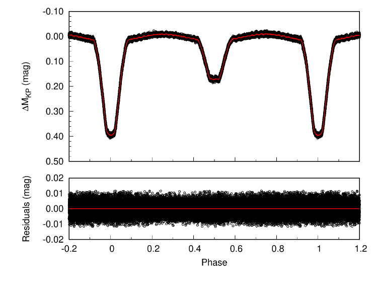
Figure 1: Light curve and O-C residuals of OO Dra. The upper panel presents the light curve (black circles), and the lower panel presents the O-C residuals. The red line in the upper panel denotes the synthesis mean curve.

Lee et al. (2018) determined physical parameters of OO Dra by using the B- and V-band photometry light curves, while observations by TESS are in white light that do not includes colour information. In this work, we adopt physical parameters obtained by Lee et al. (2018). Using the ephemerides given by Lee et al. (2018), we computed phases and folded the light curve as illustrated in Figure 1.

In order to remove the light changes due to eclipses, and obtain the pulsational light variations, we adopt a simple approach, i.e., computing a mean curve for the folded the light curve and then subtracting it from the two-minute cadence data. When computing the mean curve, the number of bins in phase should not be too large so as to ensure that each bin can contain enough data points. Given that the 58.28 day’s TESS data of OO Dra include 35927 data points, we use 1500 bins in phase in this work. Moreover, we also use 500 bins and 1000 bins in phase for the folded the light curve, which will result in slightly different wiggles. However, we find those differences and interpolation algorithms do not impact the extracted frequencies. In Figure 1, we show the mean curve with the red line in the upper panel, and show the light residuals in plots of magnitude versus phase in the lower panel. Afterwards, we perform a multiple frequency analysis of the light residuals with the software Period04 (Lenz $\&$ Breger 2005) to investigate the pulsation nature in details. No peaks higer than 100 day^-1 are found, thus we perform further frequency extractions in the range of 0$-$100 day^-1.

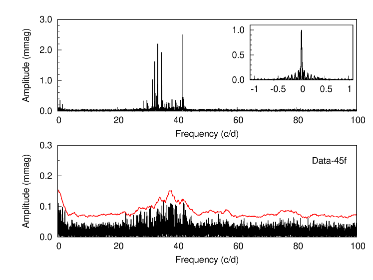
Figure 2: Fourier amplitude spectrum of the light residuals for OO Dra. The upper panel shows the original spectrum. The inset panel in the upper panel presents the window spectrum. The lower panel shows the residual spectrum after the 45 detected frequencies were subtracted. The red line denotes the level of S/N = 4.

At each step of the iteration, we pick out the frequency with the highest amplitude and carry out a multi-period least-square fit to the data using all frequencies that have been already detected. The data are then pre-whitened and the residuals were used for further analysis. Following Breger et al. (1993), we adopt the empirical threshold of the signal-to-noise ratio S/N = 4 for a frequency to be accepted as significant. Finally, we extracted a total of 45 frequencies with S/N $>$ 4, and listed them in Table 1. The uncertainties of frequencies and amplitudes are calculated using Monte Carlo simulations as described in Fu et al. (2013), and noises are computed in the range of 2 day^-1 around each frequency. Figure 2 depicts Fourier amplitude spectra of the light residuals, with the original spectrum illustrated in the upper panel and the residual spectrum of the 45 frequencies after pre-whitening illustrated in the lower panel.

Following Pápics et al. (2012) and Kurtz et al. (2015), we examine the extracted frequencies to search for the possible orbital harmonics and liner combinations in the form of $f_{i}=f_{j}\pm mf_{\rm orb}$ or $f_{i}=mf_{j}+nf_{k}$, where $f_{j}$ and $f_{k}$ are the parent frequencies, $f_{i}$ is the combination term, $m$ and $n$ are integers, and $f_{\rm orb}$ = 0.8075 day^-1. We accepted a peak as a combination if the amplitudes of both parent frequencies are larger than that of the presumed combination term, and the difference between the observed frequency and the predicted frequency is smaller than the frequency resolution 1.5/$\Delta$T= 0.027 day^-1 (Loumos $\&$ Deeming 1978). We identify a total of 33 such frequencies, and mark them in Table 1. Besides, we accepted the lower amplitude frequency as an unresolved peak if two frequencies are closer than 1.5/$\Delta$T= 0.027 day^-1. Finally, seven confident independent frequencies $f_{1}$, $f_{2}$, $f_{3}$, $f_{4}$, $f_{7}$, $f_{11}$, and $f_{12}$ are retained as shown in Table 1.

3 Input physics

Our models are computed with the one-dimensional stellar evolution code Modules for Experiments in Stellar Astrophysics (MESA, version 10398, Paxton et al. 2011, 2013, 2015, 2018). In particular, we use its submodule ”pulse$\_$adipls” to generate evolutionary models of stars and calculate the corresponding adiabatic frequencies (Christensen-Dalsgaard 2008).

In the calculations, we choose the 2005 update of the OPAL equation of state tables (Rogers & Nayfonov 2002). We adopt the OPAL opacity tables of Iglesias & Rogers (1996) in high temperatures region, and use tables of Ferguson et al. (2005) in the low temperature region. The solar metal composition AGSS09 (Asplund et al. 2009) is used as the initial ingredient in metal, and a simple photosphere is adopted for the atmospheric surface boundary conditions. The classical mixing length theory of B$\ddot{\rm o}$hm-Vitense (1958) with the solar value of $\alpha$ = 1.9 (Paxton et al. 2013) is used in the convective region. In addition, we do not consider effects of the stellar rotation, the element diffusion, and the convective overshooting, as well as magnetic fields on the structure and evolution of the star in our models (for more details, referring to the Appendix).

4 Asteroseismic analysis

4.1 Single-star Evolutiuonary Models

Our single-star evolutionary grid considers variations of the stellar mass $M$, the helium abundance $Y$, and the metallicity $Z$, which dictate the evolutionary track of a star. Therein, the stellar mass $M$ varies from 1.80 $M_{\odot}$ to 2.20 $M_{\odot}$ in an interval of 0.02 $M_{\odot}$, and metallicities $Z$ varies from 0.005 to 0.030 in an interval of 0.001. For the helium abundance $Y$, we adopt three different values: the extremely helium-poor abundance 0.220, the moderate helium abundance $0.249+1.33Z$ (Li et al. 2018) as a function of $Z$, and the helium-rich abundance 0.300.

Each star in the grid is computed evolving from pre-main sequence stage to the evolutionary status where the central hydrogen of the star exhausts ($X_{c}<$ 1$\times$10^-5). Based on the results of binary model given by Lee et al. (2018), we use 8000 K $<T_{\rm eff}<$ 8600 K and 1.95 $R_{\odot}$ $<$ $R$ $<$ 2.15 $R_{\odot}$ as the observational constraints. When a star evolves along its evolutionary track, we calculate adiabatic frequencies of the radial oscillations ($\ell=0$) and nonradial oscillations with $\ell$ = 1 and 2 for all stellar models that meet with the observational constraint. Beacuse of the cancellation effects of the surface geometry, oscillation modes with higher degree are hardly visible, thus oscillation modes with $\ell\geq 3$ are not included in this work.

In general, the component stars in binaries rotate along with the orbital motion. Following Chen et al. (2020), we consider the rotation period $P_{\rm rot}$ of the star as the fourth adjustable parameter, varying from 1.0 days to 1.50 days with a step of 0.01 days. According to the theory of stellar oscillations, rotation will result in that each nonradial oscillation mode with $\ell$ splits into $2\ell+1$ different frequencies. The general expression of the first-order effect of rotation on pulsation was deduced to be

$$\nu_{\ell,n,m}=\nu_{\ell,n}+m\delta\nu_{\ell,n}=\nu_{\ell,n}+\beta_{\ell,n}\frac{m}{P_{\rm rot}}$$ (1)

(Aerts et al. 2010). In the equation, $\ell$, $n$, and $m$ are three indices that characterize oscillation modes, and $\delta\nu_{\ell,n}$ is the splitting frequency. According to equation (1), the effect of the rotation on pulsation can be completely dictated by the constant $\beta_{\ell,n}$. Aerts et al. (2010) derived the general expression of $\beta_{\ell,n}$ to be

$$\beta_{\ell,n}=\frac{\int_{0}^{R}(\xi_{r}^{2}+L^{2}\xi_{h}^{2}-2\xi_{r}\xi_{h}-\xi_{h}^{2})r^{2}\rho dr}{\int_{0}^{R}(\xi_{r}^{2}+L^{2}\xi_{h}^{2})r^{2}\rho dr},$$ (2)

where $\xi_{r}$ is the radial displacement, $\xi_{h}$ is the horizontal displacement, $\rho$ is the local density of the star, and $L^{2}=\ell(\ell+1)$. According to the above analyses, each dipole mode splits into three different frequencies with $m$ = -1, 0, and +1, respectively, and each quadrupole mode splits into five different frequencies with $m$ = -2, -1, 0, +1, and +2, respectively.

Then we compare frequencies between models and observations according to

$$S^{2}=\frac{1}{k}\sum(|\nu_{\rm mod,i}-\nu_{\rm obs,i}|^{2}),$$ (3)

in which $\nu_{\rm mod,i}$ and $\nu_{\rm obs,i}$ represent a pair of matched model-observed frequencies, and $k$ is the number of the observed frequencies. Because of no preconceived idea of identifications of the $\delta$ Scuti frequencies, we adopt the random fitting algorithm, and consider the model frequency nearest to observations as the most probably matched model counterpart.

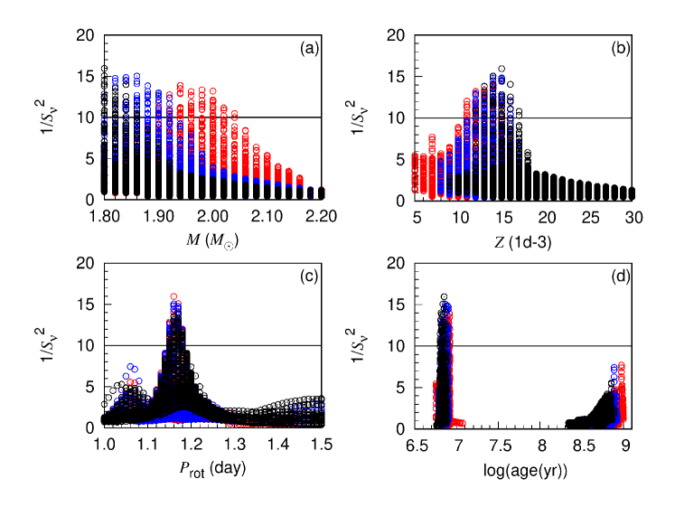
Figure 3: Plots of fitting results $S_{\rm m}^{2}$ as a function of $M$, $Z$, $P_{\rm rot}$, and the age of single-star evolutionary models, respectively. The circles in red, blue and black correspond to theoretical models with $Y$ = 0.220, 0.249+1.33$Z$, and 0.300, respecitively. The horizontal lines show the position of $S_{\rm m}^{2}$ = 0.10.

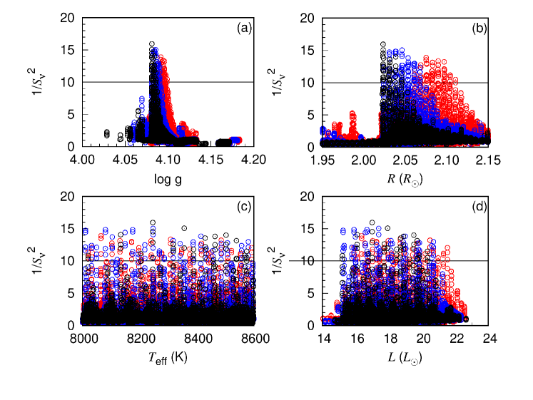
Figure 4: Plots of fitting results $S_{\rm m}^{2}$ versus global parameters of single-star evolutionary models: $\log g$, $R$, $T_{\rm eff}$, and $L$, respectively. The circles in red, blue, and black correspond to theoretical models with $Y$ = 0.220, 0.249+1.33$Z$, and 0.300, respecitively. The horizontal lines show the position of $S_{\rm m}^{2}$ = 0.10.

Figures 3 and 4 show plots of fitting results $S_{\rm m}^{2}$ versus various physical parameters. In the figures, circles in red, blue, and black are used to mark theoretical models with $Y$ = 0.220, 0.249+1.33$Z$, and 0.300, respecitively. Similar to Chen et al. (2016), we find that the solution concentrates on a small parameter space for a given evolutionary track. Thus we pick out the one model with the minimum value of $S^{2}$ along the evolutionary track, and denote the minimum value with the symbol $S_{\rm m}^{2}$. We use horizontal lines to mark the position of $S^{2}_{\rm m}$ = 0.10, which corresponds to the square of the frequency resolution $1.5/\Delta T$.

Figures 3(a) depicts the plot of $S_{\rm m}^{2}$ versus the stellar mass $M$. It can be clearly seen in the figure that theoretical models with poorer helium abundance has higher mass, i.e., 1.80$-$1.86 $M_{\odot}$ for $Y$ = 0.300, 1.80$-$1.92 $M_{\odot}$ for $0.249+1.33Z$, and 1.90$-$2.04 $M_{\odot}$ for $Y$ = 0.220, respectively. Lee et al. (2018) determined the mass of the primary star to be 2.03 $\pm$ 0.06 $M_{\odot}$. We therefore consider the 61 models with $Y=0.220$ above the horizontal line as our preferred models, and list them in Table 2. Among these models, Model A44 has the minimum value of $S_{\rm m}^{2}$, we then pick out it as the optimal single-star evolutionary model in this work.

Figures 3(b) and 3(c) depict plots of $S_{\rm m}^{2}$ versus the metallicity $Z$ and the rotational period $P_{\rm rot}$, respectively. In the figures, we noticed that values of $Z$ and $P_{\rm rot}$ show excellent convergence. Values of $Z$ converge well to 0.014${}^{+0.001}_{-0.003}$, and those of $P_{\rm rot}$ converge well to 1.17${}^{+0.01}_{-0.02}$ days.

Figure 3(d) depicts the plot of $S_{\rm m}^{2}$ as a function of the age of the star. As illustrated in the figure, ages of all preferred models converge well to $8.22^{+0.12}_{-1.33}$ Myr. Similar to KIC 10736223 (Chen et al. 2020), the primary component of OO Dra also looks like an almost unevolved star near zero-age main sequence. We therefore identify OO Dra to be another binary system that has just past a rapid mass-transfer stage.

Figures 4(a)-(d) present plots of $S_{\rm m}^{2}$ as a function of various global stellar parameters, $\log g$, $R$, $T_{\rm eff}$, and $L$, respectively. Values of $\log g$ and $R$ converge to 4.092${}^{+0.007}_{-0.004}$ and 2.075${}^{+0.035}_{-0.014}$ $R_{\odot}$, respectively. The convergence of $T_{\rm eff}$ and $L$ are relatively worse, i.e., $T_{\rm eff}$ = 8065${}^{+528}_{-45}$ K and $L$ = 16.37${}^{+5.17}_{-0.47}$ $L_{\odot}$.

Finally, fundamental physical parameters of the primary star yielded by asteroseismic fittings of single stars are listed in the second column of Table 3. Table 4 lists model frequencies of the best-fitting single-star evolutionary model, and Table 5 shows comparisons between the observed frequencies and their corresponding model counterparts. Based on the comparisons, $f_{2}$, $f_{7}$ and $f_{11}$ are identified as three dipole modes, and $f_{1}$, $f_{3}$, $f_{4}$, and $f_{12}$ as four quadrupole modes. Furthermore, we find that $f_{7}$ and $f_{2}$ are $m$ = -1 and 0 components of one triplet, and $f_{12}$ and $f_{1}$ are $m$ = +1 and +2 components of one quintuplet.

4.2 Mass-accreting Models

In Section 4.1, we analyzed the fitting results of single-star evolutionary models and found that OO Dra might be another binary system that has just undergone a rapid mass-transfer stage. Given that there are many uncertainties in binary evolution models, especially for the mass-transfer process, we model the mass-transfer process in a simlar approach with the work of Chen et al. (2020). We evolve a single star to the position where the rapid mass-transfer process may occur ( Case A or Case B binary evolution, Han et al. 2000; Chen et al. 2017), and then artificially accrete mass at a rate of 10^-6 $M_{\odot}$yr^-1 until masses of the accretor up to the given values. We considered the initial mass $M_{1}$ of the accretor between 0.40 $M_{\odot}$ and 1.00 $M_{\odot}$ in an interval of 0.1 $M_{\odot}$, and the final mass $M_{2}$ of the accretor between 1.90 $M_{\odot}$ and 2.20 $M_{\odot}$ in an interval of 0.02 $M_{\odot}$. For each pair of them, we adopt two schemes of the mass accretion, i.e., starting at the age of 0.5 Gyr (the donor on the main sequence stage, Case A binary evolution) and 1.0 Gyr (the central hydrogen of the donor exhaustion, Case B binary evolution). Moreover, the fitting results of single-star evolutionary models indicate that the primary component of OO Dra is a helium-poor star. The primordial cosmological helium abundance is determined by Planck Collaboration et al. (2016) to be 0.249. Therefore, we choose the moderate helium abundace 0.249+1.33$Z$ as the base helium abundance of the accretor, and adopt a helium-poor mass accretion, i.e., accreting 0.85 times of the base helium abundance to the surface of the accretor. In addition, we consider $Z$ between 0.005 and 0.030 in an interval of 0.001, and $P_{\rm rot}$ between 1.00 days and 1.50 days in an interval of 0.01 days.

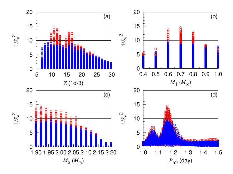
Figure 5: Plots of fitting results $S_{\rm m}^{2}$ as a function of various adjustable parameter of mass-accreting models: the metallicity $Z$, the initial mass $M_{1}$, the final mass $M_{2}$, and the rotation period $P_{\rm rot}$, respectively. The circles in red and blue correspond to accreting models of Case A and Case B evolutionary scenario, respecitively. The horizontal lines shows the position of $S_{\rm m}^{2}$ = 0.10.

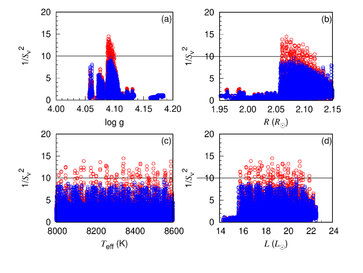
Figure 6: Plots of fitting results $S_{\rm m}^{2}$ versus stellar parameters of mass-accreting models: $\log g$, $R$, $T_{\rm eff}$, and $L$, respectively. The circles in red and blue correspond to accreting models of Case A and Case B evolutionary scenario, respecitively. The horizontal lines show the position of $S_{\rm m}^{2}$ = 0.10.

We compare frequencies between model and observations accroding to equation (3), and show changes of $S_{\rm m}^{2}$ as a function of various physical parameters of the mass-accreting models in Figures 5 and 6. In the figures, circles in red and blue correspond to accreting models of Case A and Case B binary evolutionary scenario, respecitively. It can be noticed in the figures that the Case A evolutionary scenario reproduces the $\delta$ Scuti frequencies better than the Case B evolutionary scenario. The circles above the horizontal lines correspond to 85 preferred models of Case A evolutionary scenario in Table 6.

Figures 5(a)-(d) present changes of fitting results $S_{\rm m}^{2}$ as a function of $Z$, $M_{1}$, $M_{2}$, and $P_{\rm rot}$, respectively. It can be clearly seen in the figures that values of them converge well to 0.011${}^{+0.006}_{-0.001}$, 0.70$\pm$ 0.1 $M_{\odot}$, 1.92${}^{+0.10}_{-0.02}$ $M_{\odot}$, and 1.16${}^{+0.02}_{-0.01}$ days, respectively.

Figures 6(a)-(d) depict changes of $S_{\rm m}^{2}$ as a function of global physical parameters $\log g$, $R$, $T_{\rm eff}$, and $L$, respectively. Therein, $\log g$ and $R$ exhibit good convergence to 4.090${}^{+0.010}_{-0.002}$ and 2.068${}^{+0.050}_{-0.007}$ $M_{\odot}$, respectively. While $T_{\rm eff}$ and $L$ cover a wide range. Values of $T_{\rm eff}$ vary from 8026 K to 8590 K and those of $L$ vary from 15.83 $L_{\odot}$ to 21.96 $L_{\odot}$. We listed the parameters in third column of Table 3, and find them meeting well with those of the single-star evolutionary models.

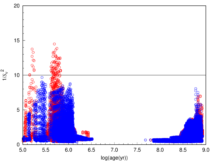
Figure 7: Plots of fitting results $S_{\rm m}^{2}$ versus tge, where tge denotes the evolutionary time of mass-accreting models since the rapid mass accretion ends. The circles in red and blue correspond to accreting models of Case A and Case B evolutionary scenario, respecitively. The horizontal lines show the position of $S_{\rm m}^{2}$ = 0.10.

Figure 7 presents changes of $S_{\rm m}^{2}$ as a function of tge of mass-accreting models, where tge is the evolutionary time since the rapid mass-accretion ends. In the figure, tge of the preferred models converge well to $0.49^{+0.18}_{-0.35}$ Myr, further confirms that OO Dra is an Algol system that has just past the rapid mass-transfer stage.

Finally, we list comparisons between model frequencies of the optimal mass-accreting model and observations in Table 7. In the table, we notice that identifications of the $\delta$ Scuti frequencies are the same with those of single-star evolutionary scenario.

5 Summary and Discussions

In this work, we presented simultaneous frequency analyses and asteroseismic modelings for the Algol-type eclipsing binary OO Dra. We performed a multiple frequency analysis of the eclipse-subtracted TESS light residuals, and obtained seven confident independent frequencies ($f_{1}$, $f_{2}$, $f_{3}$, $f_{4}$, $f_{7}$, $f_{11}$, and $f_{12}$). Therein, $f_{1}$ and $f_{3}$ have been detected by Zhang et al. (2014) from B- and V-band pulsational light curves, while $f_{2}$, $f_{4}$, $f_{7}$, $f_{11}$, and $f_{12}$ are five new frequencies not detected before. These frequencies range from 32.4538 cycle days^-1 to 41.8669 cycle days^-1, the $\delta$ Sct-type pulsational nature of OO Dra is further confirmed.

Two grids of theoretical models, the single-star evolutionary model grid and the mass-accreting model grid, are computed to reproduce the seven $\delta$ Scuti frequencies. Due to no preconceived idea of mode identifications of the $\delta$ Scuti frequencies, a random fitting algorithm is adopted in this work. Fitting results of mass-accreting models are found to agree well with those of single-star evolutionary models. Fundamental physical parameters of the primary star yielded by asteroseismology are $M$ = $1.92^{+0.10}_{-0.02}$ $M_{\odot}$, $Z$ = 0.011${}^{+0.006}_{-0.001}$, $R$ = $2.068^{+0.050}_{-0.007}$ $R_{\odot}$, $\log g$ = $4.090^{+0.010}_{-0.002}$, $T_{\rm eff}$ = $8346^{+244}_{-320}$ K, $L$ = $18.65^{+3.31}_{-2.82}$ $L_{\odot}$, which match well the results of binary model given by Lee et al. (2018).

The primary component of OO Dra is found to be almost an unevolved star near the zero-age main sequence. Ages of the primary star are determined to be $8.22^{+0.12}_{-1.33}$ Myr for single-star evolutionary models. Values of tge are determined to be $0.49^{+0.18}_{-0.35}$ for mass-accreting models. Considering that OO Dra is a detached system with the cool secondary almost filling its Roche lobe (Zhang et al. 2014; Lee et al. 2018), OO Dra may be another Algol system that has just undergone a rapid mass-transfer stage.

Besides, our asteroseismic results show that OO Dra is an Algol-type eclipsing binary formed through a helium-poor mass accretion in Case A binary evolutionary scenario. Figures 8(a) and 8(b) show profiles of Brunt$-$V$\ddot{\rm a}$is$\ddot{\rm a}$l$\ddot{\rm a}$ frequency $N$, characteristic acoustic frequencies $S_{\ell}$ ($\ell$ = 1 and 2), and hydrogen abundance $X_{\rm H}$ in the best-fitting single-star model (Model A44) and mass-accreting model (Model B21), respectively. As shown in the figures, the dominant difference between the two models is the three bumps in $N$ inside the mass-accreting model. In particular, we find that bumps 1 and 2 result from the evolution of the star, while the highest bump3 is caused by the elemental abundance gradient left behind during the process of helium-poor mass accretion. The seven $\delta$ Scuti frequencies of OO Dra are found to be p modes, which mainly propagate in the envelope of the star. However for the three bumps, they are not located in the p-mode propagation zones where $\omega^{2}>N^{2}$ and $\omega^{2}>S_{\ell}^{2}$. No frequency can reach to the bumps, that is to say, the $\delta$ Scuti frequencies are not qualified to distinguish those bumps. Furthermore, we introduce an important asteroseismic parameter, the acoustic radius $\tau_{0}$, which is the sound travel time between the surface and the center of the star. The acoustic radius $\tau_{0}$ is usually used to characterize properties of the stellar envelope (Ballot et al. 2004; Miglio et al. 2010; Chen et al. 2016), and defined by Aerts et al. (2010) as

$$\tau_{0}=\int_{0}^{R}\frac{dr}{c_{s}}.$$ (4)

In the equation, $c_{\rm s}$ is the adiabatic sound speed and $R$ is the stellar radius. The acoustic radius $\tau_{0}$ yielded by asteroseismic fittings of mass-accreting models is 2.315${}^{+0.009}_{-0.013}$ hr, which agree well with the value 2.304${}^{+0.020}_{-0.003}$ hr of single-star evolutionary models. In the Hertzsprung–Russell diagram, the instability strip of $\delta$ Scuti stars largely overlaps with that of $\gamma$ Dor stars (Balona 2011; Henry et al. 2011; Uytterhoeven et al. 2011; Xiong et al. 2016). The $\gamma$ Dor-type pulsations allow us to probe the interiors of the star, such as chemical mixing (Miglio et al. 2008) and rotation (Van Reeth et al. 2015, 2016, 2018). The $\delta$ Sct-$\gamma$ Dor hybrid behavior is found to be common for A- and F-type stars (Grigahcène et al. 2010; Balona et al. 2015). A number of eclipsing binaires with hybrid pulsators have been identified and analyzed, such as KIC 9592855 (Guo et al. 2017), KIC 7385478 (Guo & Li 2019), KIC 8113154 (Zhang et al. 2019), KIC 9850387 (Zhang et al. 2020). Due to the presence of both p and g modes, eclipsing binaries with hybrid $\delta$ Sct-$\gamma$ Dor pulsators will be very promising objects to understand the influences of mass transfer processes.

Finally, the rotaion period $P_{\rm rot}$ of the primary star is determined to be $1.17^{+0.01}_{-0.02}$ days for single-star evolutionary models and $1.16^{+0.02}_{-0.01}$ days for mass-accreting models. The spin of the primary star is slightly faster than the synchronous value. Saio (1981) and Dziembowski & Goode (1992) derived that the first-order effect of rotation on pulsation is in proportion to $1/P_{\rm rot}$, and the second-order effect on pulsation is in proportion to $1/(P_{\rm rot}^{2}\nu_{\ell,n})$. The ratio is deduced to be in the order of $1/(P_{\rm rot}\nu_{\ell,n})$. For OO Dra, $\nu_{\ell,n}$ varies from 32.4538 day^-1 to 41.8669 day^-1. The second-order effect of rotation on pulsation is much less than that of the first-order one. Therefore, the second-order effect of rotation on pulsation is not ncluded in this work.

Appendix A Inlist files used in this work (Version 10398)

A.1 The inlsit file for single-star evolution

!inlist1
&star_job
 astero_just_call_my_extras_check_model = .true.
 show_log_description_at_start = .false.
 create_pre_main_sequence_model = .true.
 change_lnPgas_flag = .true.
 new_lnPgas_flag = .true.
 change_initial_net = .true.
 new_net_name = ’o18_and_ne22.net’
 kappa_file_prefix = ’a09’
 kappa_lowT_prefix = ’lowT_fa05_a09p’
 initial_zfracs = 6
/!end of star_job namelist
&controls
 initial_mass = 1.94
 initial_z = 0.014
 initial_y = 0.220

 MLT_option = ’ML1’
 mixing_length_alpha = 1.90
 calculate_Brunt_N2 = .true.
 use_brunt_gradmuX_form = .true.
 which_atm_option = ’simple_photosphere’ !default

 max_number_backups = 50
 max_number_retries = 100
 max_model_number = 80000
 history_interval = 1
 xa_central_lower_limit_species(1) = ’h1’
 xa_central_lower_limit(1) = 1d-5
 max_num_profile_models = 80000

 use_other_mesh_functions = .true.
 mesh_delta_coeff = 0.90
 M_function_weight = 50
 max_center_cell_dq = 1d-10
 Lnuc_div_L_zams_limit = 0.95d0
 max_allowed_nz = 80000
 varcontrol_target = 1d-5
 max_years_for_timestep = 1d6 !for main sequence models (1d3 for pre-main sequence models)
/!end of controls namelist

A.2 The inlsit file for mass accretion from $M_{1}$ to $M_{2}$

!inlist2
&star_job
 show_log_description_at_start = .false.
 create_pre_main_sequence_model = .true.
 save_model_when_terminate = .true.
 save_model_filename = ’final_mass.mod’
 change_lnPgas_flag = .true.
 new_lnPgas_flag = .true.
 change_initial_net = .true.
 new_net_name = ’o18_and_ne22.net’
 kappa_file_prefix = ’a09’
 kappa_lowT_prefix = ’lowT_fa05_a09p’
 initial_zfracs = 6
/!end of star_job namelist
&controls
 initial_mass = 0.70
 initial_z = 0.011
 initial_y = 0.26363

 MLT_option = ’ML1’
 mixing_length_alpha =    1.90
 calculate_Brunt_N2 =.true.
 use_brunt_gradmuX_form = .true.
 radiation_turbulence_coeff = 0
 which_atm_option = ’simple_photosphere’ !default

 max_number_backups = 50
 max_number_retries = 100
 max_model_number = 80000
 history_interval = 1
 max_num_profile_models = 80000

 use_other_mesh_functions= .true.
 mesh_delta_coeff = 0.90
 M_function_weight = 50
 max_center_cell_dq = 1d-10
 max_allowed_nz = 80000
 varcontrol_target = 1d-5
 max_years_for_timestep = 1d6 !5d3 if star_age > 5d8

 mass_change = 1d-6 !if star_age > 5d8
 accrete_same_as_surface = .false. !if star_age > 5d8
 accrete_given_mass_fractions = .false. !if star_age > 5d8
 accretion_h1 = 0.7649145 !if star_age > 5d8
 accretion_h2 = 0d0 !if star_age > 5d8
 accretion_he3 = 0d0 !if star_age > 5d8
 accretion_he4 = 0.2240855 !if star_age > 5d8
 accretion_zfracs = 6 !if star_age > 5d8
 star_mass_max_limit = 1.92
/!end of controls namelist

A.3 The inlsit file for evolution of the accreted models

!inlist3
&star_job
 astero_just_call_my_extras_check_model = .true.
 show_log_description_at_start = .false.
 load_saved_model = .true.
 saved_model_name = ’final_mass.mod’
 new_lnPgas_flag = .true.
 change_initial_net = .true.
 new_net_name = ’o18_and_ne22.net’
 kappa_file_prefix = ’a09’
 kappa_lowT_prefix = ’lowT_fa05_a09p’
 initial_zfracs = 6
 set_initial_age = .true.
 initial_age = 0
/!end of star_job namelist
&controls
 initial_mass = 1.92
 initial_z = 0.011
 initial_y = 0.26363

 MLT_option = ’ML1’
 mixing_length_alpha = 1.90
 calculate_Brunt_N2 =.true.
 use_brunt_gradmuX_form = .true.
 which_atm_option = ’simple_photosphere’ !default

 max_number_backups = 50
 max_number_retries = 100
 max_model_number = 80000
 history_interval = 1
 max_num_profile_models = 80000
 xa_central_lower_limit_species(1) = ’h1’
 xa_central_lower_limit(1) = 1d-5

 use_other_mesh_functions= .true.
 mesh_delta_coeff = 0.90
 M_function_weight = 50
 max_allowed_nz = 80000
 max_center_cell_dq = 1d-10
 varcontrol_target = 1d-5
 max_years_for_timestep = 1d6 !for main sequence models (1d3 for pre-main sequence models)
/!end of controls namelist

Figure 8: Visualization of Brunt$-$V$\ddot{\rm a}$is$\ddot{\rm a}$l$\ddot{\rm a}$ frequency $N$, characteristic acoustic frequencies $S_{\ell}$ ($\ell$ = 1 and 2), and hydrogen abundance $X_{\rm H}$ inside the star. The upper panel presents their profiles in the single-star evolutionary model (Molde A44) and the lower panel shows the profiles in mass-accreting model (Molde B21).

Table 1: The detected frequencies of OO Dra extracted from the TESS photometric data. The columns called ID present the serial number of the detected frequencies. The columns named Freq. show detected frequencies in units of cycle per day and $\mu$Hz, respectively. The columns named Ampl. present their corresponding amplitude. The columns named S/N present their signal-to-noise. The remake columns show possible identifications for the detected frequencies.

ID	Freq.	Freq.	Ampl.	S/N	Remark	ID	Freq.	Freq.	Ampl.	S/N	Remark
	(day-1)	($\mu$Hz)	($\pm$ 24.0$\mu$mag)				(day-1)	($\mu$Hz)	($\pm$ 24.0$\mu$mag)
$f_{1}$	41.8669(4)	484.571(5)	2512.5	59.2		$f_{24}$	0.8206(53)	9.497(61)	234.2	5.1	unresolved peak
$f_{2}$	33.4728(5)	387.417(6)	2208.9	28.0		$f_{25}$	1.6316(52)	18.884(60)	220.8	6.6	$2f_{\rm orb}$
$f_{3}$	34.7407(6)	402.092(7)	1936.3	37.4		$f_{26}$	35.8564(55)	415.004(63)	221.1	6.7	$f_{7}+4f_{\rm orb}$
$f_{4}$	32.4538(7)	375.622(8)	1633.9	19.7		$f_{27}$	41.2325(54)	477.228(63)	215.2	5.9	$f_{22}+2f_{\rm orb}$
$f_{5}$	31.6572(11)	366.402(13)	1022.8	25.9	$f_{4}-f_{\rm orb}$	$f_{28}$	36.3512(58)	420.732(67)	213.8	5.9	$f_{3}+2f_{\rm orb}$
$f_{6}$	33.2641(17)	385.001(19)	694.0	13.4	$f_{4}+f_{\rm orb}$	$f_{29}$	32.5265(57)	376.465(66)	203.8	7.3	$f_{1}+f_{5}-f_{12}$
$f_{7}$	32.6314(20)	377.678(23)	583.7	14.8		$f_{30}$	40.2481(62)	465.835(71)	191.6	5.4	$f_{1}-2f_{\rm orb}$
$f_{8}$	35.0878(25)	406.109(28)	458.4	9.9	$f_{2}+2f_{\rm orb}$	$f_{31}$	30.2401(63)	350.002(73)	190.1	7.0	$f_{2}-4f_{\rm orb}$
$f_{9}$	33.1256(26)	383.398(30)	448.6	13.4	$f_{3}-2f_{\rm orb}$	$f_{32}$	37.1563(66)	430.049(77)	184.4	4.8	$f_{3}+3f_{\rm orb}$
$f_{10}$	34.8789(29)	403.690(34)	411.2	10.3	$f_{4}+3f_{\rm orb}$	$f_{33}$	29.8866(73)	345.910(84)	179.5	7.5	$f_{3}-6f_{\rm orb}$
$f_{11}$	38.2527(31)	442.740(36)	383.9	9.1		$f_{34}$	0.7706(69)	8.919(80)	175.8	4.4	unresolved peak
$f_{12}$	41.0008(35)	474.546(41)	381.3	10.1		$f_{35}$	0.8445(65)	9.774(75)	183.3	4.9	unresolved peak
$f_{13}$	39.3842(31)	455.836(35)	368.7	8.9	$f_{12}-2f_{\rm orb}$	$f_{36}$	41.0152(81)	474.713(94)	171.9	5.5	unresolved peak
$f_{14}$	0.7938(33)	9.188(38)	364.7	7.8	$f_{\rm orb}$	$f_{37}$	40.6132(81)	470.060(94)	150.1	5.0	$f_{29}+10f_{\rm orb}$
$f_{15}$	29.8652(37)	345.662(43)	359.9	10.8	$f_{2}+f_{11}-f_{1}$	$f_{38}$	32.3152(80)	374.019(93)	148.3	6.2	$f_{3}-3f_{\rm orb}$
$f_{16}$	28.5868(33)	330.865(38)	348.3	14.4	$f_{7}-5f_{\rm orb}$	$f_{39}$	38.6316(82)	447.125(94)	149.1	4.2	$f_{1}-4f_{\rm orb}$
$f_{17}$	34.9245(37)	404.219(43)	309.5	8.6	$f_{3}+f_{7}-f_{4}$	$f_{40}$	34.6681(93)	401.251(108)	137.6	4.4	$f_{23}-6f_{\rm orb}$
$f_{18}$	36.5401(41)	422.918(47)	288.8	6.0	$f_{17}+2f_{\rm orb}$	$f_{41}$	36.2091(105)	419.087(121)	129.8	4.3	$f_{1}-7f_{\rm orb}$
$f_{19}$	30.0423(43)	347.712(49)	274.4	9.2	$f_{4}-3f_{\rm orb}$	$f_{42}$	39.5323(123)	457.550(142)	124.8	4.4	unresolved peak
$f_{20}$	37.1334(46)	429.784(54)	271.4	5.7	$f_{15}+9f_{\rm orb}$	$f_{43}$	34.5243(108)	399.587(125)	123.9	4.1	$f_{12}-8f_{\rm orb}$
$f_{21}$	37.5477(43)	434.580(50)	275.2	6.6	$2f_{8}-f_{7}$	$f_{44}$	41.4923(104)	480.236(121)	119.3	4.0	$f_{11}+4f_{\rm orb}$
$f_{22}$	39.6148(42)	458.504(49)	255.0	6.7	$f_{1}+f_{7}-f_{10}$	$f_{45}$	35.4024(112)	409.750(129)	117.6	4.2	$f_{1}-8f_{\rm orb}$
$f_{23}$	39.5176(55)	457.379(63)	249.7	7.3	$f_{3}+f_{11}-f_{2}$

Table 2: Preferred models with $S_{\rm m}^{2}$ $\leq$ 0.10. $P_{\rm rot}$ represents the rotation period, $\tau_{0}$ represnets the acoustic radius, and $X_{\rm c}$ represents the mass fraction of hydrogen in the center of the star.

Model	$P_{\rm rot}$	$Z$	$M$	$Y$	$T_{\rm eff}$	log$g$	$R$	$L$	$\tau_{0}$	$X_{\rm c}$	Age	$S_{\rm m}^{2}$
	(day)		($M_{\odot}$)		(K)	(cgs)	$(R_{\odot})$	($L_{\odot}$)	(hr)		(Myr)
A01	1.15	0.013	1.94	0.220	8172	4.091	2.076	17.27	2.308	0.767	7.93	0.098
A02	1.15	0.013	1.96	0.220	8241	4.093	2.083	17.98	2.311	0.767	7.75	0.094
A03	1.15	0.013	2.00	0.220	8376	4.096	2.097	19.44	2.317	0.767	7.41	0.099
A04	1.15	0.014	1.94	0.220	8065	4.091	2.076	16.38	2.305	0.766	8.22	0.090
A05	1.15	0.014	1.96	0.220	8131	4.093	2.083	17.04	2.307	0.766	8.04	0.088
A06	1.15	0.015	1.96	0.220	8020	4.093	2.082	16.12	2.302	0.765	8.34	0.097
A07	1.16	0.011	2.00	0.220	8593	4.096	2.097	21.54	2.324	0.769	6.88	0.098
A08	1.16	0.012	1.94	0.220	8277	4.091	2.076	18.18	2.313	0.768	7.64	0.094
A09	1.16	0.012	1.96	0.220	8347	4.093	2.083	18.93	2.316	0.768	7.47	0.090
A10	1.16	0.012	1.98	0.220	8417	4.094	2.090	19.69	2.317	0.768	7.30	0.091
A11	1.16	0.012	2.00	0.220	8486	4.096	2.097	20.48	2.320	0.768	7.14	0.082
A12	1.16	0.012	2.02	0.220	8554	4.097	2.104	21.30	2.322	0.768	6.99	0.090
A13	1.16	0.013	1.90	0.220	8034	4.088	2.062	15.91	2.303	0.767	8.30	0.095
A14	1.16	0.013	1.92	0.220	8103	4.090	2.069	16.58	2.305	0.767	8.11	0.081
A15	1.16	0.013	1.94	0.220	8172	4.091	2.076	17.27	2.308	0.767	7.93	0.077
A16	1.16	0.013	1.96	0.220	8241	4.093	2.083	17.98	2.311	0.767	7.75	0.076
A17	1.16	0.013	1.98	0.220	8309	4.094	2.090	18.70	2.313	0.767	7.58	0.079
A18	1.16	0.013	2.00	0.220	8376	4.096	2.097	19.44	2.317	0.767	7.41	0.084
A19	1.16	0.013	2.02	0.220	8443	4.097	2.104	20.20	2.318	0.767	7.25	0.090
A20	1.16	0.013	2.04	0.220	8509	4.099	2.110	20.98	2.321	0.767	7.09	0.095
A21	1.16	0.014	1.94	0.220	8065	4.092	2.075	16.37	2.304	0.766	8.22	0.074
A22	1.16	0.014	1.96	0.220	8131	4.093	2.083	17.04	2.307	0.766	8.04	0.076
A23	1.16	0.014	1.98	0.220	8198	4.095	2.089	17.71	2.309	0.766	7.86	0.083
A24	1.16	0.014	2.00	0.220	8263	4.096	2.097	18.41	2.313	0.766	7.69	0.096
A25	1.16	0.015	1.96	0.220	8020	4.093	2.082	16.11	2.301	0.765	8.34	0.088
A26	1.17	0.011	1.94	0.220	8379	4.091	2.076	19.08	2.317	0.769	7.36	0.096
A27	1.17	0.011	1.96	0.220	8451	4.093	2.083	19.88	2.318	0.769	7.20	0.088
A28	1.17	0.011	1.98	0.220	8522	4.094	2.090	20.70	2.321	0.769	7.04	0.086
A29	1.17	0.011	2.00	0.220	8593	4.096	2.097	21.54	2.324	0.769	6.88	0.083
A30	1.17	0.012	1.90	0.220	8135	4.088	2.062	16.73	2.306	0.768	8.00	0.099
A31	1.17	0.012	1.92	0.220	8206	4.090	2.069	17.44	2.309	0.768	7.82	0.092
A32	1.17	0.012	1.94	0.220	8278	4.091	2.075	18.17	2.312	0.768	7.64	0.089
A33	1.17	0.012	1.96	0.220	8348	4.093	2.083	18.92	2.315	0.768	7.47	0.085
A34	1.17	0.012	1.98	0.220	8417	4.094	2.090	19.69	2.317	0.768	7.30	0.079
A35	1.17	0.012	2.00	0.220	8486	4.096	2.097	20.48	2.320	0.768	7.14	0.076
A36	1.17	0.012	2.02	0.220	8554	4.097	2.104	21.30	2.322	0.768	6.99	0.092
A37	1.17	0.013	1.90	0.220	8034	4.089	2.061	15.90	2.302	0.767	8.30	0.083
A38	1.17	0.013	1.92	0.220	8103	4.090	2.069	16.58	2.305	0.767	8.11	0.078
A39	1.17	0.013	1.94	0.220	8172	4.091	2.076	17.27	2.308	0.767	7.93	0.078
A40	1.17	0.013	1.96	0.220	8241	4.093	2.083	17.98	2.311	0.767	7.75	0.079
A41	1.17	0.013	1.98	0.220	8309	4.094	2.090	18.70	2.313	0.767	7.58	0.075
A42	1.17	0.013	2.00	0.220	8376	4.096	2.097	19.44	2.317	0.767	7.41	0.091
A43	1.17	0.013	2.02	0.220	8443	4.097	2.104	20.20	2.318	0.767	7.25	0.098
A44	1.17	0.014	1.94	0.220	8065	4.092	2.075	16.37	2.304	0.766	8.22	0.072
A45	1.17	0.014	1.96	0.220	8132	4.093	2.082	17.03	2.306	0.766	8.04	0.085
A46	1.17	0.014	1.98	0.220	8198	4.095	2.089	17.71	2.309	0.766	7.86	0.086
A47	1.17	0.015	1.96	0.220	8020	4.093	2.082	16.11	2.301	0.765	8.34	0.095
A48	1.18	0.011	1.96	0.220	8451	4.093	2.083	19.88	2.318	0.769	7.20	0.094
A49	1.18	0.011	1.98	0.220	8522	4.094	2.090	20.70	2.321	0.769	7.04	0.088
A50	1.18	0.011	2.00	0.220	8593	4.096	2.097	21.54	2.324	0.769	6.88	0.088
A51	1.18	0.012	1.92	0.220	8207	4.090	2.068	17.44	2.308	0.768	7.82	0.098
A52	1.18	0.012	1.94	0.220	8278	4.091	2.075	18.17	2.312	0.768	7.64	0.091
A53	1.18	0.012	1.96	0.220	8348	4.093	2.083	18.92	2.315	0.768	7.47	0.088
A54	1.18	0.012	1.98	0.220	8417	4.094	2.090	19.69	2.317	0.768	7.30	0.087
A55	1.18	0.012	2.00	0.220	8486	4.096	2.097	20.48	2.320	0.768	7.14	0.089
A56	1.18	0.013	1.90	0.220	8034	4.089	2.061	15.90	2.302	0.767	8.30	0.089
A57	1.18	0.013	1.92	0.220	8104	4.090	2.068	16.57	2.304	0.767	8.11	0.090
A58	1.18	0.013	1.94	0.220	8173	4.092	2.075	17.26	2.307	0.767	7.93	0.090
A59	1.18	0.013	1.96	0.220	8241	4.093	2.082	17.97	2.310	0.767	7.75	0.092
A60	1.18	0.013	1.98	0.220	8309	4.094	2.090	18.70	2.313	0.767	7.58	0.091
A61	1.18	0.014	1.94	0.220	8065	4.092	2.075	16.37	2.304	0.766	8.22	0.090

Table 3: Fundamental parameters of the primary component of OO Dra yielded by asteroseismology. $P_{\rm rot}$ is the rotation period. $\tau_{0}$ represents the acoustic radius. $X_{\rm c}$ denotes the mass fraction of hydrogen in the center of the star. Tge denotes the evolutionary time of mass-accreting models since the rapid mass accretion ends. Stellar parameters of Lee et al. (2018) by the binary model are listed in the last column.

Parameters	Single-star models	Mass-accreting models	Lee et al. (2018)
$Z$	0.011$-$0.015 (0.014${}_{-0.003}^{+0.001}$)	0.010-0.017 (0.011${}_{-0.001}^{+0.006}$)
$M$ ($M_{\odot}$)	1.90$-$2.04 (1.94${}_{-0.04}^{+0.10}$)	$\cdots$	2.031$\pm$0.058
$Y$	0.220	0.249+1.33$Z$
$M_{1}$ ($M_{\odot}$)	$\cdots$	0.60-0.80 (0.70$\pm$ 0.10)
$M_{2}$ ($M_{\odot}$)	$\cdots$	1.90-2.02 (1.92${}_{-0.02}^{+0.10}$)
$P_{\rm rot}$(day)	1.15-1.18 ($1.17^{+0.01}_{-0.02}$)	1.15-1.18 (1.16${}_{-0.01}^{+0.02}$)
$T_{\rm eff}$ (K)	8020-8593 ($8065^{+528}_{-45}$)	8026-8590 (8346${}_{-320}^{+244}$)	8260$\pm$210
$\log g$ (cgs)	4.088-4.099 ($4.092^{+0.007}_{-0.004}$)	4.088-4.100 (4.090${}_{-0.002}^{+0.010}$)	4.110$\pm$0.017
$R$ ($R_{\odot}$)	2.061-2.110 ($2.075^{+0.035}_{-0.014}$)	2.061-2.118 (2.068${}_{-0.007}^{+0.050}$)	2.078$\pm$0.026
$L$ ($L_{\odot}$)	15.90-21.54 ($16.37^{+5.17}_{-0.47}$)	15.83-21.96 (18.65${}_{-2.82}^{+3.31}$)	18.0$\pm$1.9
$\tau_{0}$ (hr)	2.301-2.324 ($2.304^{+0.020}_{-0.003}$)	2.302-2.324 (2.315${}_{-0.013}^{+0.009}$)
$X_{\rm c}$	0.765-0.769 (0.766${}^{+0.003}_{-0.001}$)	0.696-0.726 (0.723${}^{+0.003}_{-0.027}$)
Age (Myr)	6.89-8.34 ($8.22^{+0.12}_{-1.33}$)
Tge (Myr)		0.14-0.67 (0.49${}^{+0.18}_{-0.35}$)

Table 4: Theoretical frequencies of the best-fitting single-star evolutionary model (Model A44). $\nu_{\rm mod}$ is the model frequency. $\ell$ and $n$ are its spherical harmonic degree and radial order, respectively. $\beta_{\ell,n}$ is the rotational parameters defined as equation (2).

$\nu_{\rm mod}(\ell,n)$	$\beta_{\ell,n}$	$\nu_{\rm mod}(\ell,n)$	$\beta_{\ell,n}$	$\nu_{\rm mod}(\ell,n)$	$\beta_{\ell,n}$
($\mu$Hz)		($\mu$Hz)		($\mu$Hz)
166.800(0,0)		124.265(1,0)	0.487	164.889(2,0)	0.918
215.551(0,1)		171.134(1,1)	0.985	191.521(2,0)	0.861
265.700(0,2)		222.486(1,2)	0.997	226.527(2,1)	0.996
315.399(0,3)		276.840(1,3)	0.998	261.773(2,2)	0.878
365.904(0,4)		332.122(1,4)	0.996	305.360(2,3)	0.879
417.999(0,5)		387.732(1,5)	0.993	357.115(2,4)	0.925
470.551(0,6)		442.375(1,6)	0.990	411.472(2,5)	0.951
523.603(0,7)		496.263(1,7)	0.989	465.420(2,6)	0.964
577.884(0,8)		550.456(1,8)	0.988	519.169(2,7)	0.972
633.391(0,9)		605.631(1,9)	0.987	573.737(2,8)	0.977
689.930(0,10)		661.736(1,10)	0.986	629.321(2,9)	0.980

Table 5: Comparisons between theoretical frequencies of the best-fitting single-star evolutionary model (Model A44) and observations. $\nu_{\rm obs}$ denotes the observed frequency. $\nu_{\rm mod}$ represents its model counterpart. $|\nu_{\rm obs}-\nu_{\rm mod}|$ shows the difference between the observed frequency and the model counterpart.

ID	$\nu_{\rm obs}$	$\nu_{\rm mod}$	($\ell$, $n$, $m$)	$|\nu_{\rm obs}-\nu_{\rm mod}|$
	($\mu$Hz)	($\mu$Hz)		($\mu$Hz)
$f_{1}$	484.571	484.493	(2, 6, +2)	0.078
$f_{2}$	387.417	387.732	(1, 5, 0)	0.315
$f_{3}$	402.092	402.064	(2, 5, -1)	0.028
$f_{4}$	375.622	375.416	(2, 4, +2)	0.206
$f_{7}$	377.678	377.909	(1, 5, -1)	0.231
$f_{11}$	442.740	442.375	(1, 6, 0)	0.365
$f_{12}$	474.546	474.957	(2, 6, +1)	0.411

Table 6: Preferred mass-accreting models with $S_{\rm m}^{2}$ $\leq$ 0.10. $P_{\rm rot}$ represents the rotation period. $\tau_{0}$ represents the acoustic radius. $X_{\rm c}$ represents the mass fraction of hydrogen in the center of the star. Tge denotes the evolutionary time of mass-accreting models since the rapid mass accretion ends.

Model	$P_{\rm rot}$	$Z$	$M_{1}$	$M_{2}$	$T_{\rm eff}$	log$g$	$R$	$L$	$\tau_{0}$	$X_{\rm c}$	Tge	$S_{\rm m}^{2}$
	(day)		($M_{\odot}$)	($M_{\odot}$)	(K)		$(R_{\odot})$	($L_{\odot}$)	(hr)		(Myr)
B01	1.15	0.010	0.70	1.94	8558	4.091	2.076	20.78	2.322	0.726	0.43	0.096
B02	1.15	0.011	0.70	1.90	8257	4.089	2.061	17.74	2.311	0.723	0.52	0.098
B03	1.15	0.011	0.70	1.92	8346	4.090	2.068	18.65	2.315	0.723	0.49	0.084
B04	1.15	0.011	0.70	1.94	8433	4.092	2.075	19.57	2.318	0.723	0.46	0.095
B05	1.15	0.011	0.70	1.96	8522	4.093	2.083	20.57	2.322	0.723	0.43	0.091
B06	1.15	0.012	0.60	1.90	8416	4.088	2.062	19.17	2.316	0.722	0.18	0.094
B07	1.15	0.012	0.60	1.92	8501	4.090	2.070	20.09	2.319	0.722	0.17	0.082
B08	1.15	0.012	0.60	1.94	8590	4.091	2.077	21.10	2.322	0.722	0.16	0.079
B09	1.15	0.012	0.70	1.90	8142	4.089	2.061	16.77	2.306	0.721	0.56	0.081
B10	1.15	0.012	0.70	1.92	8227	4.090	2.068	17.60	2.309	0.721	0.53	0.085
B11	1.15	0.012	0.70	1.94	8312	4.091	2.076	18.47	2.313	0.721	0.50	0.092
B12	1.15	0.012	0.70	2.00	8563	4.096	2.097	21.24	2.322	0.721	0.41	0.094
B13	1.15	0.013	0.60	1.94	8476	4.091	2.076	19.99	2.318	0.720	0.14	0.099
B14	1.15	0.013	0.70	1.90	8026	4.089	2.061	15.83	2.302	0.719	0.59	0.087
B15	1.15	0.013	0.70	1.92	8108	4.090	2.067	16.60	2.305	0.719	0.56	0.100
B16	1.15	0.013	0.70	1.94	8191	4.092	2.075	17.41	2.309	0.719	0.53	0.091
B17	1.16	0.010	0.70	1.90	8375	4.089	2.061	18.78	2.314	0.726	0.49	0.091
B18	1.16	0.010	0.70	1.92	8467	4.090	2.068	19.75	2.318	0.726	0.46	0.084
B19	1.16	0.010	0.70	1.94	8558	4.091	2.076	20.78	2.322	0.726	0.43	0.085
B20	1.16	0.011	0.70	1.90	8257	4.089	2.061	17.74	2.311	0.723	0.52	0.078
B21	1.16	0.011	0.70	1.92	8346	4.090	2.068	18.65	2.315	0.723	0.49	0.069
B22	1.16	0.011	0.70	1.94	8433	4.092	2.075	19.57	2.318	0.723	0.46	0.075
B23	1.16	0.011	0.70	1.96	8522	4.093	2.083	20.57	2.322	0.723	0.43	0.089
B24	1.16	0.012	0.60	1.90	8416	4.088	2.062	19.17	2.316	0.722	0.18	0.083
B25	1.16	0.012	0.60	1.92	8501	4.090	2.070	20.09	2.319	0.722	0.17	0.075
B26	1.16	0.012	0.60	1.94	8590	4.091	2.077	21.10	2.322	0.722	0.16	0.073
B27	1.16	0.012	0.70	1.90	8142	4.089	2.061	16.77	2.306	0.721	0.56	0.072
B28	1.16	0.012	0.70	1.92	8227	4.090	2.068	17.60	2.309	0.721	0.53	0.073
B29	1.16	0.012	0.70	1.94	8312	4.091	2.076	18.47	2.313	0.721	0.50	0.094
B30	1.16	0.012	0.70	1.96	8396	4.093	2.082	19.35	2.315	0.721	0.47	0.090
B31	1.16	0.012	0.70	2.00	8563	4.096	2.097	21.24	2.322	0.721	0.41	0.089
B32	1.16	0.013	0.60	1.94	8476	4.091	2.076	19.99	2.318	0.720	0.14	0.100
B33	1.16	0.013	0.70	1.90	8026	4.089	2.061	15.83	2.302	0.719	0.59	0.088
B34	1.16	0.013	0.70	1.92	8108	4.090	2.067	16.60	2.305	0.719	0.56	0.090
B35	1.16	0.013	0.70	1.94	8191	4.092	2.075	17.41	2.309	0.719	0.53	0.092
B36	1.16	0.016	0.80	1.96	8179	4.093	2.084	17.45	2.309	0.698	0.60	0.096
B37	1.16	0.016	0.80	1.98	8262	4.094	2.091	18.30	2.312	0.698	0.57	0.094
B38	1.16	0.016	0.80	2.00	8344	4.095	2.098	19.16	2.315	0.698	0.53	0.090
B39	1.16	0.016	0.80	2.02	8427	4.097	2.105	20.07	2.318	0.698	0.50	0.089
B40	1.16	0.017	0.80	1.96	8049	4.093	2.083	16.37	2.303	0.696	0.65	0.080
B41	1.16	0.017	0.80	1.98	8128	4.094	2.090	17.13	2.306	0.696	0.62	0.085
B42	1.16	0.017	0.80	2.00	8207	4.096	2.097	17.93	2.309	0.696	0.58	0.095
B43	1.16	0.017	0.80	2.02	8285	4.097	2.104	18.74	2.312	0.696	0.55	0.097
B44	1.17	0.010	0.70	1.90	8375	4.089	2.061	18.78	2.314	0.726	0.49	0.085
B45	1.17	0.010	0.70	1.92	8467	4.090	2.068	19.75	2.318	0.726	0.46	0.079
B46	1.17	0.010	0.70	1.94	8558	4.091	2.076	20.78	2.322	0.726	0.43	0.096
B47	1.17	0.011	0.70	1.90	8257	4.089	2.061	17.74	2.311	0.723	0.52	0.079
B48	1.17	0.011	0.70	1.92	8346	4.090	2.068	18.65	2.315	0.723	0.49	0.075
B49	1.17	0.011	0.70	1.94	8433	4.092	2.075	19.57	2.318	0.723	0.46	0.076
B50	1.17	0.011	0.70	1.96	8522	4.093	2.082	20.55	2.320	0.723	0.44	0.093

Table 7: Comparisons between model frequencies and observations for the best-fitting model (Model B21) in mass-accreting evolutionary grid. $\nu_{\rm obs}$ denotes the observed frequency. $\nu_{\rm mod}$ denotes the model frequency. $|\nu_{\rm obs}-\nu_{\rm mod}|$ is the difference between the observed frequency and its model counterpart.

ID	$\nu_{\rm obs}$	$\nu_{\rm mod}$	($\ell$, $n$, $m$)	$|\nu_{\rm obs}-\nu_{\rm mod}|$
	($\mu$Hz)	($\mu$Hz)		($\mu$Hz)
$f_{1}$	484.571	484.464	(2, 6, +2)	0.107
$f_{2}$	387.417	387.756	(1, 5, 0)	0.339
$f_{3}$	402.092	401.898	(2, 5, -1)	0.194
$f_{4}$	375.622	375.656	(2, 4, +2)	0.034
$f_{7}$	377.678	377.848	(1, 5, -1)	0.170
$f_{11}$	442.740	442.294	(1, 6, 0)	0.446
$f_{12}$	474.546	474.846	(2, 6, +1)	0.300

Table 8: Table 6 - continued

Model	$P_{\rm rot}$	$Z$	$M_{1}$	$M_{2}$	$T_{\rm eff}$	log$g$	$R$	$L$	$\tau_{0}$	$X_{\rm c}$	Tge	$S_{\rm m}^{2}$
	(day)		($M_{\odot}$)	($M_{\odot}$)	(K)		$(R_{\odot})$	($L_{\odot}$)	(hr)		(Myr)
B51	1.17	0.012	0.60	1.90	8416	4.088	2.062	19.17	2.316	0.722	0.18	0.093
B52	1.17	0.012	0.60	1.92	8501	4.090	2.070	20.09	2.319	0.722	0.17	0.089
B53	1.17	0.012	0.60	1.94	8590	4.091	2.077	21.10	2.322	0.722	0.16	0.088
B54	1.17	0.012	0.70	1.90	8142	4.089	2.061	16.77	2.306	0.721	0.56	0.085
B55	1.17	0.012	0.70	1.92	8227	4.090	2.068	17.60	2.309	0.721	0.53	0.083
B56	1.17	0.012	0.70	1.94	8311	4.092	2.075	18.45	2.312	0.721	0.50	0.098
B57	1.17	0.012	0.70	1.96	8396	4.093	2.082	19.35	2.315	0.721	0.47	0.097
B58	1.17	0.015	0.80	1.98	8389	4.094	2.091	19.46	2.316	0.700	0.52	0.097
B59	1.17	0.015	0.80	2.02	8561	4.097	2.106	21.39	2.323	0.700	0.46	0.091
B60	1.17	0.016	0.80	1.92	8013	4.090	2.069	15.86	2.302	0.698	0.67	0.094
B61	1.17	0.016	0.80	1.94	8097	4.091	2.076	16.65	2.305	0.698	0.63	0.085
B62	1.17	0.016	0.80	1.96	8179	4.093	2.084	17.45	2.309	0.698	0.60	0.081
B63	1.17	0.016	0.80	1.98	8262	4.094	2.091	18.30	2.312	0.698	0.57	0.080
B64	1.17	0.016	0.80	2.00	8344	4.095	2.098	19.16	2.315	0.698	0.53	0.079
B65	1.17	0.016	0.80	2.02	8427	4.097	2.105	20.07	2.318	0.698	0.50	0.084
B66	1.17	0.016	0.80	2.04	8509	4.098	2.111	20.99	2.320	0.698	0.47	0.097
B67	1.17	0.016	0.80	2.06	8590	4.100	2.118	21.96	2.324	0.698	0.45	0.095
B68	1.17	0.017	0.80	1.96	8049	4.093	2.083	16.37	2.303	0.696	0.65	0.081
B69	1.17	0.017	0.80	1.98	8128	4.094	2.090	17.13	2.306	0.696	0.62	0.081
B70	1.17	0.017	0.80	2.00	8206	4.096	2.097	17.91	2.308	0.696	0.58	0.096
B71	1.17	0.017	0.80	2.02	8285	4.097	2.104	18.74	2.312	0.696	0.55	0.099
B72	1.18	0.010	0.70	1.90	8375	4.089	2.061	18.78	2.314	0.726	0.49	0.099
B73	1.18	0.010	0.70	1.92	8467	4.090	2.068	19.75	2.318	0.726	0.46	0.094
B74	1.18	0.011	0.70	1.90	8257	4.089	2.061	17.74	2.311	0.723	0.52	0.100
B75	1.18	0.011	0.70	1.94	8433	4.092	2.075	19.57	2.318	0.723	0.46	0.097
B76	1.18	0.015	0.80	1.98	8389	4.094	2.091	19.46	2.316	0.700	0.52	0.098
B77	1.18	0.015	0.80	2.02	8561	4.097	2.106	21.39	2.323	0.700	0.46	0.098
B78	1.18	0.016	0.80	1.92	8013	4.090	2.069	15.86	2.302	0.698	0.67	0.094
B79	1.18	0.016	0.80	1.94	8097	4.091	2.076	16.65	2.305	0.698	0.63	0.090
B80	1.18	0.016	0.80	1.96	8179	4.093	2.084	17.45	2.309	0.698	0.60	0.086
B81	1.18	0.016	0.80	1.98	8262	4.094	2.091	18.30	2.312	0.698	0.57	0.087
B82	1.18	0.016	0.80	2.00	8344	4.095	2.098	19.16	2.315	0.698	0.53	0.087
B83	1.18	0.016	0.80	2.02	8427	4.097	2.105	20.07	2.318	0.698	0.50	0.099
B84	1.18	0.017	0.80	1.96	8049	4.093	2.083	16.35	2.302	0.696	0.65	0.094
B85	1.18	0.017	0.80	1.98	8128	4.094	2.090	17.13	2.306	0.696	0.62	0.097

References

- Aerts et al. (2010) Aerts, C., Christensen-Dalsgaard, J., & Kurtz, D. W. 2010, Asteroseismology, Astronomy and Astrophysics Library (Berlin: Springer)
- Aerts & Harmanec (2004) Aerts, C., & Harmanec, P. 2004, Spectroscopically and Spatially Resolving the Components of the Close Binary Stars, 325
- Asplund et al. (2009) Asplund, M., Grevesse, N., Sauval, A. J., & Scott, P. 2009, ARA&A, 47, 481
- Ballot et al. (2004) Ballot, J., Turck-Chièze, S., & García, R. A. 2004, A&A, 423, 1051
- Balona (2011) Balona, L. A. 2011, MNRAS, 415, 1691
- Balona et al. (2015) Balona, L. A., Daszyńska-Daszkiewicz, J., & Pamyatnykh, A. A. 2015, MNRAS, 452, 3073
- Beck et al. (2014) Beck, P. G., Hambleton, K., Vos, J., et al. 2014, A&A, 564, A36
- Beck et al. (2018) Beck, P. G., Kallinger, T., Pavlovski, K., et al. 2018, A&A, 612, A22
- Biyalieva & Khruslov (2007) Biyalieva, N. A. & Khruslov, A. V. 2007, Peremennye Zvezdy Prilozhenie, 7, 17
- Böhm-Vitense (1958) Böhm-Vitense, E. 1958, ZAp, 46, 108
- Bowman et al. (2019) Bowman, D. M., Johnston, C., Tkachenko, A., et al. 2019, ApJ, 883, L26
- Breger et al. (1993) Breger, M., Stich, J., Garrido, R., et al. 1993, A&A, 271, 482
- Chen et al. (2017) Chen, X. F., Maxted, P. F. L., Li, J., et al. 2017, MNRAS, 467, 1874
- Chen et al. (2016) Chen, X. H., Li, Y., Lai, X. J., & Wu, T. 2016, A&A, 593, A69
- Chen et al. (2020) Chen, X. H.,Zhang, X. B., Li, Y., et al. 2020, ApJ, 895, 136
- Christensen-Dalsgaard (2008) Christensen-Dalsgaard, J. 2008, Ap&SS, 316, 113
- Dimitrov et al. (2008) Dimitrov, D., Kraicheva, Z., & Popov, V. 2008, Information Bulletin on Variable Stars, 5842, 1
- Dziembowski & Goode (1992) Dziembowski, W. A., & Goode, P. R. 1992, ApJ, 394, 670
- Ferguson et al. (2005) Ferguson, J. W., Alexander, D. R., Allard, F., et al. 2005, ApJ, 623, 585
- Fu et al. (2013) Fu, J. N., Dolez, N., Vauclair, G., et al. 2013, MNRAS, 429, 1585
- Gaulme et al. (2013) Gaulme, P., McKeever, J., Rawls, M. L., et al. 2013, ApJ, 767, 82
- Gaulme et al. (2014) Gaulme, P., Jackiewicz, J., Appourchaux, T., et al. 2014, ApJ, 785, 5
- Gaulme et al. (2016) Gaulme, P., McKeever, J., Jackiewicz, J., et al. 2016, ApJ, 832, 121
- Gaulme & Guzik (2019) Gaulme, P., & Guzik, J. A. 2019, A&A, 630, A106
- Gizon & Solanki (2003) Gizon, L., & Solanki, S. K. 2003, ApJ, 589, 1009
- Grigahcène et al. (2010) Grigahcène, A., Antoci, V., Balona, L., et al. 2010, ApJ, 713, L192
- Guo et al. (2017) Guo, Z., Gies, D. R., & Matson, R. A. 2017, ApJ, 851, 39
- Guo & Li (2019) Guo, Z. & Li, G. 2019, ApJ, 882, L5
- Han et al. (2000) Han, Z., Tout, C. A., & Eggleton, P. P. 2000, MNRAS, 319, 215
- Henry et al. (2011) Henry, G. W., Fekel, F. C., & Henry, S. M. 2011, AJ, 142, 39
- Ibanoglu et al. (2018) Ibanoglu, C., Çakırlı, Ö., & Sipahi, E. 2018, New A, 62, 70
- Iglesias & Rogers (1996) Iglesias, C. A., & Rogers, F. J. 1996, ApJ, 464, 943
- Jenkins et al. (2016) Jenkins, J. M., Twicken, J. D., McCauliff, S., et al. 2016, Society of Photo-Optical Instrumentation Engineers(SPIE) Conference Series, Vol. 9913, The TESS scienceprocessing operations center, 99133E
- Kahraman Aliçavuş et al. (2017) Kahraman Aliçavuş, F., Soydugan, E., Smalley, B., & Kubát, J. 2017, MNRAS, 470, 915
- Kurtz et al. (2015) Kurtz, D. W., Shibahashi, H., Murphy, S. J., et al. 2015, MNRAS, 450, 3015
- Lee et al. (2018) Lee, J. W., Hong, K., Koo, J.-R., et al. 2018, AJ, 155, 5
- Lenz & Breger (2005) Lenz, P., & Breger, M. 2005, Communications in Asteroseismology, 146, 53
- Li et al. (2018) Li, T., Bedding, T. R., Huber, D., et al. 2018, MNRAS, 475, 981
- Liakos & Niarchos (2017) Liakos, A., & Niarchos, P. 2017, MNRAS, 465, 1181
- Loumos & Deeming (1978) Loumos, G. L., & Deeming, T. J. 1978, Ap&SS, 56, 285
- Maceroni et al. (2013) Maceroni, C., Montalbán, J., Gandolfi, D., et al. 2013, A&A, 552, A60
- Miglio et al. (2008) Miglio, A., Montalbán, J., Noels, A., & Eggenberger, P. 2008, MNRAS, 386, 1487
- Miglio et al. (2010) Miglio, A., Montalbán, J., Carrier, F., et al. 2010, A&A, 520, L6
- Mkrtichian et al. (2005) Mkrtichian, D. E., Rodríguez, E., Olson, E. C., et al. 2005, in ASP Conf. Ser. 197, Tidal Evolution and Oscillations in Binary Stars, ed. A. Claret, A. Gimenez, & J.-P. Zahn (San Francisco CA : ASP), 197
- Mkrtichian et al. (2007) Mkrtichian, D. E., Kim, S.-L., Rodríguez, E., et al. 2007, in ASP Conf. Ser.194, Solar and Stellar Physics Through Eclipses, ed. O. Demircan,S. O. Selam, & B. Albayrak (San Francisco, CA: ASP), 194
- Pápics (2012) Pápics, P. I. 2012, Astronomische Nachrichten, 333, 1053
- Paxton et al. (2011) Paxton, B., Bildsten, L., Dotter, A., et al. 2011, ApJS, 192, 3
- Paxton et al. (2013) Paxton, B., Cantiello, M., Arras, P., et al. 2013, ApJS, 208, 4
- Paxton et al. (2015) Paxton, B., Marchant, P., Schwab, J., et al. 2015, ApJS, 220, 15
- Paxton et al. (2018) Paxton, B., Schwab, J., Bauer, E. B., et al. 2018, ApJS, 234, 34
- Planck Collaboration et al. (2016) Planck Collaboration, Ade, P. A. R., Aghanim, N., et al. 2016, A&A, 594, A13
- Rogers & Nayfonov (2002) Rogers, F. J., & Nayfonov, A. 2002, ApJ, 576, 1064
- Ruciński (1969) Ruciński, S. M. 1969, Acta Astron., 19, 245
- Saio (1981) Saio, H. 1981, ApJ, 244, 299
- Schmid & Aerts (2016) Schmid, V. S., & Aerts, C. 2016, A&A, 592, A116
- Slawson et al. (2011) Slawson, R. W., Prša, A., Welsh, W. F., et al. 2011, AJ, 142, 160
- Uytterhoeven et al. (2011) Uytterhoeven, K., Moya, A., Grigahcène, A., et al. 2011, A&A, 534, A125
- Van Reeth et al. (2015) Van Reeth, T., Tkachenko, A., Aerts, C., et al. 2015, A&A, 574, A17
- Van Reeth et al. (2016) Van Reeth, T., Tkachenko, A., & Aerts, C. 2016, A&A, 593, A120
- Van Reeth et al. (2018) Van Reeth, T., Mombarg, J. S. G., Mathis, S., et al. 2018, A&A, 618, A24
- Xiong et al. (2016) Xiong, D. R., Deng, L., Zhang, C., & Wang, K. 2016, MNRAS, 457, 3163
- Zhang et al. (2014) Zhang, X. B., Deng, L. C., Tian, J. F., et al. 2014, AJ, 148, 106
- Zhang et al. (2018) Zhang, X. B., Fu, J. N., Luo, C. Q., Ren, A. B., & Yan, Z. Z. 2018, ApJ, 865, 115
- Zhang et al. (2019) Zhang, X. B., Wang, K., Chen, X. H., et al. 2019, ApJ, 884, 165
- Zhang et al. (2020) Zhang, X. B., Chen, X. H., Zhang, H. T., et al. 2020, ApJ, 895, 124.