Transit Origami: A Method to Coherently Fold Exomoon Transits in Time Series Photometry

Abstract

One of the simplest ways to identify an exoplanetary transit is to phase fold a photometric time series upon a trial period - leading to a coherent stack when using the correct value. Such phase-folded transits have become a standard data visualisation in modern transit discovery papers. There is no analogous folding mechanism for exomoons, which would have to represent some kind of double-fold; once for the planet and then another for the moon. Folding with the planet term only, a moon imparts a small decrease in the surrounding out-of-transit averaged intensity, but its incoherent nature makes it far less convincing than the crisp stacks familiar to exoplanet hunters. Here, a new approach is introduced that can be used to achieve the transit origami needed to double fold an exomoon, in the case where a planet exhibits TTVs. This double fold has just one unknown parameter, the satellite-to-planet mass ratio, and thus a simple one-dimensional grid search can be used to rapidly identify power associated with candidate exomoons. The technique is demonstrated on simulated light curves, exploring the breakdown limits of close-in and/or inclined satellites. As an example, the method is deployed on Kepler-973b, a warm mini-Neptune exhibiting an 8 minute TTV, where the possibility that the TTVs are caused by a single exomoon is broadly excluded, with upper limits probing down to a Ganymede-sized moon.

1 Introduction

The detection of a transiting planet within a photometric time series has become a mature science after more than two decades of practice (Charbonneau et al., 2000; Henry et al., 2000) and many thousands of successes (see NASA Exoplanet Archive; Akeson et al. 2013). Although in rare cases transits are identified by eye (e.g. Wang et al. 2013), most detections have resulted from automated algorithms - with the so-called “Box Least Squares” (BLS) algorithm (Kovács, Zucker, & Mazeh, 2002) being perhaps the most well-known. Modifications to this approach continue to be developed (e.g. TLS; Hippke & Heller 2019), but the core principle remains unchanged - fold a transit light curve upon a trial period and examine the result for a coherent, short-duty cycle dip.

A folded transit light curve does not have higher signal-to-noise ratio (SNR) than the original ensemble of $N$ transits. When compared to a single (unfolded) transit, the folded transit representation decreases the noise ($\sigma$) at each phase point from $\sigma\to\sigma/\sqrt{N}$ (for Gaussian statistics). Thus, the folded transit is $\sqrt{N}$ times more precise than a single transit. In contrast, whilst the unfolded original time series has the original noise $\sigma$, it contains $N$ times more transits than a single transit. Thus, the ensemble, unfolded time series yields a transit precision $\sqrt{N}$ times more precise than a single transit. In principle then, there is no difference in overall SNR between the two, but a single high SNR folded transit is more visually impactful than a train of lower SNR transits. Yet more, a folded transit immediately allows one to assess whether the signal is coherent, as expected for a transiting planet (an incoherent fold would higher scatter in the signal region caused by, for example, varying transit depths). For these reasons, the folded transit light curve is a common way of visualising new detections, to such an extent it has arguably become a standardised accompanying visual.

Exomoon transits do not have an equivalent folding mechanism in the existing literature. The basic challenge is that if one folds upon the planetary period, the companion moon(s) will be in different relative phases in each epoch. Thus, the moon transits are incoherent when phase-folded in the standard manner. Despite being incoherent, their presence is still felt in the light curve. As eluded to earlier, incoherent signals yield higher scatter and indeed this was proposed by Simon et al. (2012) as a possible pathway towards their detection - seeking increased scatter in the regions surrounding the planetary transit. In practice, Hippke (2015) report that the act of masking transits during the necessary light curve detrending means that the regions bracketing the transits are least accurately detrended, which consequently imparts artificial excess scatter into this region.

As an alternative, Heller (2014) suggested focusing on measuring the mean flux, rather than the scatter (which was dubbed the “orbital sampling effect”, OSE). Although the moon(s) indeed moves between different positions yielding an incoherent phase-folded signal, it should slightly decrease the average flux within the pre- and post-transit regions surrounding the planetary transit imparting a broadly symmetric signature. Crucially though, as discussed in Teachey, Kipping, & Schmitt (2018), a moon must spend less than half of its time in each region (as it will spend a finite amount of time overlapping with the planetary transit), which means that this averaging process must be accomplished with an arithmetic mean rather than a median. Medians offer a robust statistic than can ignore the influence of outlier transits being stacked together, but because a median is the 50th percentile position in a sorted list, it would remove the effect of an exomoon in the outlined procedure. A remedy could be to mirror the phase-folded transits prior to averaging, although this would sacrifice the distinctive symmetric feature expected from this method. Despite the outlined progress then, exomoon hunters still lack the kind of compelling visual of a planetary transit fold that our exoplanet colleagues enjoy.

The true power of the conventional light curve fold is the fact that it produces a coherent, clean stacked transit, with a well-resolved ingress, egress and “flat-bottom”. Although certainly astrophysical false-positives exist here, the actual reality of some kind of photometric dip is far less ambiguous than that present with the exomoon approaches discussed thus far. In this work, a possible resolution to this is introduced, which subtly folds the light curve in a novel way to recover a coherent moon transit. The paper is organised as follows. In Section 2, the underlying theory and concept is introduced along with a suggested recipe. In Section 3, the expected SNR is estimated using the technique to aid the community in quickly calculating detectability. In Section 4, numerical tests of the method are demonstrated, exploring the impact of inclination effects. In Section 5, the method is applied to a real transiting planet, Kepler-973b, where an exomoon is excluded down to Ganymede-radius. Finally, the limitations of this method, as well as possible future development and extensions, are discussed in Section 6.

2 Introducing the Double-Fold

2.1 Predicting the position of an exomoon

To begin, consider the transit timing variations (TTVs) imparted upon a planet by a single satellite, or indeed one large dominant moon. A simple depiction of a planet-moon system transiting a star is shown in Figure 1 to guide the reader for what follows.

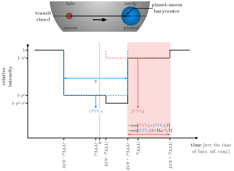
Figure 1: Simplified depiction of a planet-moon pair transiting a star. A coplanar configuration is shown here for simplicity, but the concept generalises to other configurations as discussed in the text. The fact that the planet transits early in this instance (versus the barycentre), reveals that the moon must be transiting late - modulo the unknown mass ratio, $M_{SP}(\equiv M_{S}/M_{P})$ term. Note that although the planet-moon pair appear at quadrature, this is only a product of the projection shown and infact the pair could be close to a conjunction.

Following Sartoretti & Schneider (1999) and Kipping (2009a), this TTV effect can be analytically derived by considering the offset of the planet away from the planet-moon barycentre divided by the relative velocity of that barycentre compared to the star. For a transiting planet with zero impact parameter, the orbit lives entirely within the $\hat{X}$-$\hat{Y}$ plane, where $\hat{Z}$ is the line-of-sight of the observer. Since transiting planets can necessarily only have small inclinations (which is defined as an $\hat{X}$-rotation conventionally), then most of motion during a transit occurs along the $\hat{X}$-direction. This property greatly simplifies the derivation, and was exploited explicitly in the derivation presented in Kipping (2011), such that

$$\mathrm{TTV}_{P}(t) =\frac{(X_{P}-X_{B})}{\big{[}\frac{\mathrm{d}X_{B}}{\mathrm{d}{t}}\big{]}_{\mathrm{inf.\,\,conj.}}},$$ (1)

where $\mathrm{TTV}_{P}(t)$ is the TTV effect experienced by the planet, $X_{P}$ is the $\hat{X}$ Cartesian element of the planet’s position (with respect to the star), $X_{B}$ is the $\hat{X}$ Cartesian element of the planet-satellite barycentre and “inf. conf.” refers to the instant of inferior conjunction.

In Kipping (2011), eccentric moon orbits are considered, but this study simplifies the analysis by limiting the scope to circular orbit moons. The close proximity of moons to their planets means that tidal forces rapidly circularise satellites (Porter & Grundy, 2011; Hamers & Portegies Zwart, 2018) and thus, unless they are being continuously excited, one should generally expect circular orbits. This also allows for considerable simplification in what follows.

The overall orbit around the star is often elliptical (Kane et al., 2012; Xie et al., 2016; Van Eylen et al., 2019). Nevertheless, if one models a transit with a circular orbit, the fits are essentially nearly identical to a full eccentric fit (Barnes, 2007). The primary difference is that the inferred value of $a/R_{\star}$ (or equivalently $\rho_{\star}$ if parametrised that way) is skewed from the true value (Kipping et al., 2012; Dawson & Johnson, 2012), which originates from the differing orbital velocity. As a result, exoplanets are well-modelled and explained by circular orbits, provided one understands that the resulting $a/R_{\star}$ values should be treated as “effective” values.

Proceeding as described then, one may start by modifying the expressions of Kipping (2011) to the limiting case of circular orbits, to obtain

$$\mathbf{R}_{B}=\begin{bmatrix}X_{B}\\ Y_{B}\\ Z_{B}\\ \end{bmatrix}=\begin{bmatrix}a_{P}\sin(n_{P}(t-t_{\mathrm{inf.\,\,conj.}}))\\ a_{P}\cos(n_{P}(t-t_{\mathrm{inf.\,\,conj.}}))\cos i_{P}\\ a_{P}\cos(n_{P}(t-t_{\mathrm{inf.\,\,conj.}}))\sin i_{P}\end{bmatrix}.$$ (2)

where $a_{P}$ is the semi-major axis of the planet-satellite barycentre around the star, $n_{P}$ its mean motion and $i_{P}$ is the orbital inclination.

The satellite’s orbit with respect to the planet-moon barycentre can be found through a series of matrix rotations, and for circular orbits becomes

$$\mathbf{R}_{SB}=\begin{bmatrix}a_{SB}\cos\Omega_{S}\sin(n_{S}(t-\tau_{S}))-\sin i_{S}\sin\Omega_{S}\cos(n_{S}(t-\tau_{S}))\\ a_{SB}\sin\Omega_{S}\sin(n_{S}(t-\tau_{S}))+\sin i_{S}\cos\Omega_{S}\cos(n_{S}(t-\tau_{S}))\\ a_{SB}\cos i_{S}\cos(n_{S}(t-\tau_{S}))\end{bmatrix}.$$ (3)

One may now write that $\mathbf{R}_{S}=\mathbf{R}_{B}+\mathbf{R}_{SB}$, and also that $\mathbf{R}_{P}=\mathbf{R}_{B}-M_{SP}\mathbf{R}_{SB}$ where $M_{SP}(\equiv M_{S}/M_{P})$ is the mass ratio between the satellite and the planet. One can now evaluate Equation (1) to give

$$\mathrm{TTV}_{P}(t)= \frac{a_{SB}M_{SP}}{a_{P}n_{P}}\Big{(}\cos(n_{S}(t-\tau_{S}))\sin i_{S}\sin\Omega_{S}$$

$$-\cos\Omega_{S}\sin(n_{S}(t-\tau_{S}))\Big{)}.$$ (4)

It’s not just the planet that experiences deviations in its position from the barycentre. The satellite too experiences deviations - indeed much larger deviations. The temporal offset of the satellite away from the time of inferior conjunction, can be found using an analogous version of Equation (1):

$$\mathrm{TTV}_{S}(t)= -\frac{a_{SB}}{a_{P}n_{P}}\Big{(}\cos(n_{S}(t-\tau_{S}))\sin i_{S}\sin\Omega_{S}$$

$$-\cos\Omega_{S}\sin(n_{S}(t-\tau_{S}))\Big{)}.$$ (5)

In fact, it is perhaps not surprising to see that Equation (4) and Equation (5) are intimately connected, via

$$\mathrm{TTV}_{S}(t) =-\frac{1}{M_{SP}}\mathrm{TTV}_{P}(t),$$ (6)

where the $t$ functionality indicates that this a fully general expression at all times, and indeed for any choice of inclination angles $i_{S}$ and $\Omega_{S}$. This is very important. If one takes a known TTV signal, which appears sinusoidal and thus moon-like, one can calculate the location of the expected moon modulo just one unknown parameter - $M_{SP}$. For a given choice of $M_{SP}$ then, one can predict where the moon should be and go further and stack those events to create a moon-folded transit light curve. It should be emphasised that such moon-folding is only possible if a TTV signal is in hand.

Despite the fact that Equation (6) is formally independent of $i_{S}$ and $\Omega_{S}$, recall that an assumption upon which its derivation is predicated is that the orbital motion of the planet and moon are predominantly in the $\hat{X}$-direction. As the orbit becomes increasingly inclined, that assumption will be stressed, making Equation (6) increasingly approximate in nature. And so, in this regime, one would expect moon-folding to still yield a signal, but attenuated to some degree as a result of this effect, which is illustrated later in numerical tests (see Section 4). In such a case, the optimal reconstruction would require a fully photodynamic algorithm (e.g. LUNA; Kipping 2011). This highlights how moon-folding is a powerful tool for initial detection but characterisation of the signal warrants other tools.

2.2 Bounds on $M_{SP}$

For a given exoplanetary TTV signal, one can propose a trial $M_{SP}$ mass ratio and then perform a light curve fold for a putative exomoon (more details on the suggested procedure are provided later in Section 2.3). Given that there is only one unknown, the problem is well-suited for a simple grid search, similar to how a periodogram used in radial velocity surveys for example (Cumming, 2004; Gregory, 2007; Zechmeister & Kürster, 2009). In that example, the range of periods to be explored is not unbounded, typically constrained by the Nyquist frequency and the baseline of observations. Similarly, the $M_{S}/M_{P}$ grid also has a physical boundary between 0 and 1. However, efficiency can be improved by further tightening these limits as argued in what follows.

For a given TTV signal, one can measure its amplitude and period straight-forwardly. The TTV amplitude is proportional to $a_{SB}M_{SP}$ (Equation 4), but the planet-moon separation cannot grow without limit - orbital stability must be considered. This allows one to define a limiting value for $M_{SP}$, following a similar logic to that used recently by Kipping & Teachey (2020) to define the maximum TTV amplitude possible due to an exomoon. Let us define the maximum allowed planet-moon separation, $a_{SP}$, as $a_{SP,\mathrm{max}}=f_{\mathrm{max}}R_{\mathrm{Hill}}$, where $f_{\mathrm{max}}$ is a value less than one and $R_{\mathrm{Hill}}$ is the planet’s Hill radius.

$$a_{SB,\mathrm{max}}= \frac{a_{SP,\mathrm{max}}}{1+M_{SP}},$$

$$\qquad= \frac{f_{\mathrm{max}}a_{P}(q/3)^{1/3}}{1+M_{SP}}.$$ (7)

Turning back to the planetary TTV signal in Equation (4), it is noted that the inclination terms in parentheses can never exceed unity, and thus

$$\mathrm{TTV}_{P}\leq \frac{a_{SB}M_{SP}}{a_{P}n_{P}}.$$ (8)

Using this, and the maximum possible planet-moon separation, allows one to estimate the lighest possible moon which could explain a given TTV amplitude:

$$M_{SP}\geq\Bigg{(}\frac{f_{\mathrm{max}}(q/3)^{1/3}}{n_{P}\mathrm{TTV}_{P}}-1\Bigg{)}^{-1}.$$ (9)

In principle, $M_{SP}$ could be up approach unity, with the greatest allowed value occurring when $a_{SP}$ takes the smallest allowed value (for example the Roche limit of the planet). However, in practice, as the planet-moon separation shrinks, one of the explicit assumptions in the TTV theory described in Kipping (2011) becomes invalid. This occurs when the moon period is comparable to the transit duration, such that the moon essentially washes out its own TTV. If one requires $P_{S}\gg T$, then one can set $P_{S}\geq gT$, where $g$ is chosen to be some number greater than unity, with 10 being suggested here (i.e. an order-of-magnitude). This can be related to planet-moon separation divided by the Hill radius, $f$, using Equation (12) of Kipping (2009a):

$$f_{\mathrm{min}} =\Bigg{(}3\Big{(}\frac{gT}{P_{P}}\Big{)}^{2}\Bigg{)}^{1/3},$$ (10)

such that

$$M_{SP}\leq\Bigg{(}\frac{f_{\mathrm{min}}(q/3)^{1/3}}{n_{P}\mathrm{TTV}_{P}}-1\Bigg{)}^{-1}.$$ (11)

2.3 The transit origami recipe

To illustrate moon-folding, a suggested toy algorithm is now introduced. However, it is highlighted that reasonable variants of some of the choices made in what follows would also produce a viable moon folding strategy.

The planetary transit will be deeper than the satellite transit and thus must be dealt with. The signal could be modelled out, but given how small moons could be, any slight residual error in that process would potentially introduce false-positives. Accordingly, it is suggested here that one should simply exclude the planetary transit altogether. A proposed recipe for achieving this is now described, which is broken down into three steps (1, 2, 3), which themselves have multiple parts (a, b, c). Beginning with step 1:

• Infer the transit time and transit shape parameter posteriors for all available epochs.

• Calculate a 2 $\sigma$ lower (upper) limit on the time of planetary first (fourth) contact for each epoch.

• For each epoch, take the detrended photometric time series and exclude all times that occurs within the 2 $\sigma$ confidence planetary transit window creating a “planet-cleansed” time series.

Having excluded the planetary transits, step 2 next finds the points expected to occur within the moon’s transit. In what follows, it is assumed that the moon transit has approximately the same duration as the planetary transit. This is suitable when the moon’s velocity, is much less than the barycentric velocity, but will become stressed for moons on tight orbits. For circular orbits, and again using Equation (12) of Kipping (2009a), this assumption corresponds to $f\gg 3(q/3)^{2/3}$ - as an example, $q=10^{-3}$ implies $f\gg 0.014$. This assumption thus only impacts the most compact moons; moons which are unsuitable for moon-folding anyway since their short periods average out their own TTVs (as well producing very small TTVs even if this wasn’t true). Accordingly, let us proceed with the following sub-steps for step 2:

• Choose a trial $M_{SP}$ value between the minimum and maximum allowed values (e.g. as part of a grid search).

• Using Equation (6), calculate a posterior distribution for each epoch’s mid-transit time for the moon.

• Add these posteriors to $\pm 0.5$ the transit duration posteriors (keeping track of mutual covariances), to calculate the expected time of the satellite’s first and fourth contact (for example by taking the median of the posteriors).

A trapezoidal shaped transit’s signal-to-noise is maximised by choosing a duration that corresponds to the FWHM (rather than the first-to-fourth contact duration; Carter et al. 2008) and thus it is suggested to employ that definition in the above. Finally, in step 3, the planet-cleansed light curve is separated into two arrays for the in- and out-of-moon transit:

• From the cleansed data, select only the times which occur inside the satellite transits. Create a second array for the other data.

• For both arrays, subtract the time of expected moon mid-transit time at an epoch-by-epoch level.

• Combine the epochs together, to create two final arrays; one for in-moon transit and one for out-of-moon transit.

Step 1 need only be done once, but steps 2 & 3 will be repeated for each choice of $M_{SP}$. Much like a periodogram, one searches through a grid of $M_{SP}$ values, creates the corresponding folded light curves, and then measures statistical quantities pertaining to signal strength and significance. This can generally be done thousands of times in minutes on a modern laptop with typical data sets.

For the statistical score quantifying significance/power, it is suggested here to use a simple box model (similar to Kovács, Zucker, & Mazeh 2002), which is then compared to the null hypothesis of a flat line. The box’s width is fixed to the planetary transit duration (as used in step 2), and the central time is also fixed for a given choice of $M_{SP}$, and thus one simply need measure the weighted average of the photometric points in and out of the putative moon dip. The null hypothesis’ flat line is the weighted sum of all points. A $\Delta\chi^{2}$ score can then be used to assess significance.

2.4 Possible future recipe improvements

It is emphasised that the suggested recipe is not the only way to conduct moon folding, but merely a simple straight-forward one that was found to work well (see Section 4). For future iterations, some possible suggested improvements are highlighted.

First, limb darkening is ignored in the above, in the same way as BLS does(Kovács, Zucker, & Mazeh, 2002). Recent work has found that $\sim 10\%$ improvements in planet search sensitivity can be achieved using a modification of BLS that accounts for limb darkening, dubbed Transit Least Squares (TLS; Hippke & Heller 2019). Similarly, it would be worthwhile to investigate this here.

Second, for a given guessed $M_{S}/M_{P}$ value, a reconstructed signal is obtained assuming the moon duration is equal to that of the planet. Since that reconstructed signal “knows” the size of the moon (given by the depth), this could be used to refine the duration slightly - as the smaller moon radius will slightly reduce the overall duration. This is a small effect but could further improve sensitivity.

Finally, although the notebooks used to generate the results in this paper are publicly available (https://github.com/CoolWorlds/TransitOrigamiBits), a clean, user-friendly open-source package would be of obvious benefit to the community.

3 Signal-to-Noise Ratio

The double-folding technique discussed in Section 2 provides a pathway to quickly flagging possible exomoon candidates for exoplanets exhibiting TTVs. One can extend the formalism to estimate the expected signal-to-noise ratio (SNR) of an exomoon relative to the planet. In what follows, an approximate method for estimating this is presented, which should not be treated as an exact calculation, but rather as an observational guide.

3.1 Mean duration of the isolated moon transits

Since the moon folding technique only uses the segments of the exomoon light curve that occur outside of the planetary transit, one needs to estimate the mean duration of these segments to make progress. From Figure 1, one can see that the portion of the exomoon transit that occurs outside of the planetary transit is given by

$$T_{S,\mathrm{out}}(t) =\mathrm{min}[|\mathrm{TTV}_{S}(t)|+|\mathrm{TTV}_{P}(t)|,T]$$ (12)

where the minimum ($\mathrm{min}$) function caps the moon duration at $T$, the duration to independently cross the stellar disk. As depicted in Figure 1, it is assumed here (as was done earlier) that the duration of the exomoon transit is the same as that of the planet, which implies the orbit is nearly coplanar and that the orbital velocity of the moon around the barycentre is much less than the orbital velocity of the barycentre around the star. This is the same assumption used in TTV theory derivations, specifically it represents assumptions $\alpha 3$ and $\alpha 4$ in the derivation presented in Kipping (2011).

Plugging Equation (6) into Equation (12), one finds

$$T_{S,\mathrm{out}}(t) =\mathrm{min}[|\mathrm{TTV}_{P}(t)|(1+M_{SP}^{-1}),T].$$ (13)

To calculate the mean duration over all times, one needs to integrate the above. The TTV waveform becomes sinusoidal is the limit of $\Omega_{S}\to 0$ (see Equation 4) which is adopted as an assumption in what follows to simplify the calculation. Replacing time, $t$, with orbital phase, $\phi\equiv n_{s}(t-\tau_{s})$, one finds $\mathrm{TTV}_{P}=-A_{\mathrm{TTV-P}}\sin(\phi)$, and thus

$$<T_{S,\mathrm{out}}> =\frac{\int_{0}^{2\pi}T_{S,\mathrm{out}}(\phi)\mathrm{d}\phi}{\int_{0}^{2\pi}\mathrm{d}\phi}.$$ (14)

The mean duration should be compared to the duration of the planetary event for context, and so it is useful to define the duration ratio $\mathcal{D}\equiv\frac{<T_{S,\mathrm{out}}>}{T}$, which can be shown to satisfy

$$\mathcal{D}(\Lambda)=\frac{2}{\pi}\begin{cases}\Lambda&\text{if }0<\Lambda\leq 1,\\ \Lambda-\sqrt{\Lambda^{2}-1}+\mathrm{sec}^{-}1[\Lambda]&\text{if }\Lambda>1,\end{cases}$$ (15)

where $\Lambda$ is defined as

$$\Lambda\equiv A_{\mathrm{TTV-P}}(1+M_{SP}^{-1})/T,$$ (16)

and $A_{\mathrm{TTV-P}}\equiv(a_{SB}M_{SP})/(a_{P}n_{P})$.

3.2 Effective SNR of the moon folded dip

Section 3.1 establishes and formulates that the moon’s isolated transit has a mean duration equal to some fraction of the full planetary duration. The SNR of this signal, relative to the planetary signal, will be scaled by the square root of this duration ratio, as well as the transit depth ratio. This can be solved for analytically under the simplifying assumptions of the expressions presented in this section.

Before doing so, it useful to re-express $\Lambda$ in terms of the exomoon’s physical parameters, rather than the planetary TTV amplitude. Expanding the equation for $A_{\mathrm{TTV-P}}$, one has

$$A_{\mathrm{TTV-P}} =\frac{a_{SB}M_{SP}}{a_{P}n_{P}},$$

$$=\frac{a_{SP}}{a_{P}n_{P}}\frac{1}{M_{SP}^{-1}+1}$$ (17)

And plugging this into Equation (18), one finds the $M_{SP}$ terms cancel to give

$$\Lambda =\Big{(}\frac{1}{2\pi}\Big{)}\Big{(}\frac{a_{SP}}{a_{P}}\Big{)}\Big{(}\frac{P}{T}\Big{)}.$$ (18)

As an alternative formulation, the $a_{SP}$ term can be replaced in the above with a moon located at $x$ planetary radii.

$$\Lambda \simeq\Big{(}\frac{xp}{2\sqrt{1-b^{2}}}\Big{)},$$ (19)

The SNR of the exomoon folded signal is now

$$\mathrm{SNR}_{S} =R_{SP}^{2}\sqrt{\mathcal{D}(\Lambda)}\mathrm{SNR}_{P}.$$ (20)

3.3 Comparison to OSE

We note that the SNR of exomoon transits for the portion of the light curve outside of the planetary transit will be approximately the same whether one uses the moon folding method (this work) or OSE (Heller, 2014). There’s no “free lunch” in an SNR-sense by simply shuffling the transits around in different ways (although small differences will occur due to approximations in the transit shape). Photodynamical modelling (e.g. LUNA; (Kipping, 2011)) will, in general, always lead to higher SNRs since it includes numerous effects ignored with both approaches; such as variable moon transit durations as a function of orbital phase, light curve asymmetry due to acceleration effects, etc.

Although OSE and moon folding produce similar SNRs, a clear advantage of moon folding is that a coherent signal is reconstructed. This allows individual epochs to be inspected for consistency with the stacked signal. One can also freely median-bin the folded light curve, producing a composite signal robust to outlier measurements - which is not possible for OSE due to the duty cycle effect discussed earlier. Moon folding also features a simple search statistic which can be sought in a 1D grid, akin to a BLS periodogram. Finally, the moon folding method recovers not only the moon’s relative size, but also its relative mass, allowing for an extra layer of statistical testing by comparison to physical models. On the downside, moon folding only works if a TTV signal is present, unlike OSE. However, high confidence exomoon detections will ultimately demand both dynamical and transit signatures regardless. Yet more, it may be possible to extend this method to non-TTV systems as discussed in Section 6.

3.4 SNR calculation for the Kepler catalog

To provide a sense of scale, Equation 20 was evaluated on the Kepler catalog. Rather than curate TTVs for each planet and attempt any kind of model selection for their potential to be a moon, let us instead simply use the $\Lambda$ formula of Equation (18). For the satellite, the Solar System moons provide a plausible set of input parameters for this calculation. Doing so, it was found that Ganymede consistently led to the most favourable SNRs and thus is adopted exclusively in what follows.

For some short-period planets, the smaller Hill spheres would place Ganymede (located at 15 planetary radii) outside of the stable orbital range. In such cases, the distance was truncated down to half a Hill sphere, where planetary masses are estimated using forecaster’s conservative lower bound (Chen & Kipping, 2017).

Only five Kepler planetary systems have predicted SNRs greater than 3 for a Ganymede moon: Kepler-93b ($\mathrm{SNR}_{S}=3.5$), KOI-314b ($\mathrm{SNR}_{S}=3.3$) Kepler-142b ($\mathrm{SNR}_{S}=6.1$), Kepler-142c ($\mathrm{SNR}_{S}=5.8$) and Kepler-142d ($\mathrm{SNR}_{S}=5.5$). KOI-314b experience a near mean-motion resonance with KOI-314c (Kipping et al., 2014) and thus although it exhibits TTVs, this would greatly complicate any attempt to extract a moon-only TTV component. Kepler-142 is an extremely compact system around a late M-dwarf (Muirhead et al., 2012), in many ways a precursor discovery to TRAPPIST-1 (Gillon et al., 2017). As a result, exomoons are improbable due to dynamical packing (Kane, 2017). This leaves the small, rocky planet Kepler-93b (Ballard et al., 2014), which could be worth future investigation although no TTVs are presently known for the system (Dulz & Reed, 2017).

4 Numerical Tests

4.1 An example system

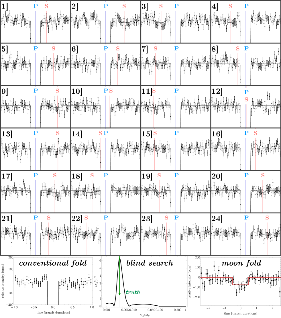
Figure 2: Panels 1] to 24] show a zoom-in of the 24 transit epochs simulated of the hypothetical Jupiter+Earth around a Sun-like star described in Section 4.1. The blue vertical lines mark the location of the planetary mid-transit time (“P”) , whereas the red mark the predicted location of the satellite (“S”) transit using Equation (6) and using the blindly recovered mass ratio, $M_{S}/M_{P}$. Bottom-left shows a simple linear fold of the transits, which is incoherent for the moon events thus making them indistinguishable from the noise. Bottom-middle shows a grid search of the $\Delta\chi^{2}$ significance of moon fold trials as a function of $M_{S}/M_{P}$, with a clear peak at the true value. Bottom-right shows the moon fold corresponding to the most significant $M_{S}/M_{P}$ value.

Before discussing a grid of tests that were performed, it is useful to begin with a single example for illustrative purposes. Consider a hypothetical test system comprising of a Jupiter-sized/mass planet orbiting a Sun-sized/radius star on a circular path with an orbital period of 60 days. The planet transits the star with an impact parameter of $0.5$, and the star has a quadratic limb darkening profile of $q_{1}=q_{2}=0.3$ (Kipping, 2013). Around this planet orbits a single Earth-sized/mass moon at the Hill radius ($f=1$) and in a coplanar, circular orbit. This means that the planet is ${\sim}317$ times more massive than the moon, such that $M_{S}/M_{P}=0.00315$.

A baseline of 4 years of photometric data was assumed, similar to that of the Kepler Mission. The light curves are generated using the photodynamic LUNA algorithm for planet-moon transits (Kipping, 2011). Uncorrelated Gaussian noise is then added to the simulated light curves; specifically, the noise is equivalent to an RMS of 52.7 ppm over 6 hours (similar to the median 6-hour CDPP for Kepler dwarfs 54.5 ppm; Christiansen et al. 2012), or 1 mmag over a minute. In total, 24 transits were generated and are shown in Figure 2.

A grid of 301 $M_{S}/M_{P}$ values were generated, separated uniformly in log-space from $10^{-3}$ to $1$. This range extends beyond the bounds described in Section 2.2, in order to provide a full inspection of the parameter space. We follow the recipe in Section 2.3 and measure the $\Delta\chi^{2}$ between a simple box-model and a flat-line at each $M_{S}/M_{P}$ trial. Since the simulated data are uniformly sampled, it is possible to derive the planetary transit time for each epoch non-parametrically by using a flux weighted centroid.

A strong, unimodal peak emerges at $M_{SP}=10^{-2.5}=0.00316$ (see Figure 2), almost exactly the same value as the truth. For the assumed noise, this is a $\Delta\chi^{2}=39.7$, or $\sqrt{\Delta\chi^{2}}=6.3$ $\sigma$ detection. It is noted that using the true photodynamic model only marginally improves this to $7.7$ $\sigma$. In other words, the assumptions inherent to moon-folding method means that it recovers 82% of the maximum possible SNR. This demonstrates how the moon-folding technique is generally expected to recover the large majority of the theoretical maximum SNR.

4.2 Varying the moon parameters

Let us next consider repeating the above but varying three of the exomoon parameters, in order to investigate their impact on the sensitivity of the moon-folding technique. This also provides an opportunity to investigate the overall changes in SNR as moon parameters are varied, since different parameter inputs will affect the amount of time the moon spends in transit (Martin, Fabrycky, & Montet, 2019). To this end, the first two parameters varied describe the orbital orientation, $i_{S}$ and $\Omega_{S}$, which are varied in $30^{\circ}$ intervals. A third parameter that is varied is $f$ in 0.1 steps, which corresponds to the exomoon semi-major axis in Hill radii. Since semi-major axis and orbital period are related via Kepler’s Third Law, then this also changes the orbital period of the moon.

In each case, the procedure described in the previous subsection is repeated and used to produce two plots (Figures 3 & 4). The first is the absolute $\Delta\chi^{2}$ change with the same assumed noise level as before, which provides an estimate of detectability and is shown in Figure 3. The second is the relative change in $\chi^{2}$ versus that found from the true photodynamic model (but using only the same planet-cleansed photometric points). This relative quantity is a useful gauge of how much of the full signal the moon-folding is able to recover and is independent of the assumed noise level (see Figure 4). Not surprisingly, the closest moon orbit considered in the $f$-grid, $f=0.1$, comes into tension with the assumption of a slow-moving moon and thus is not used.

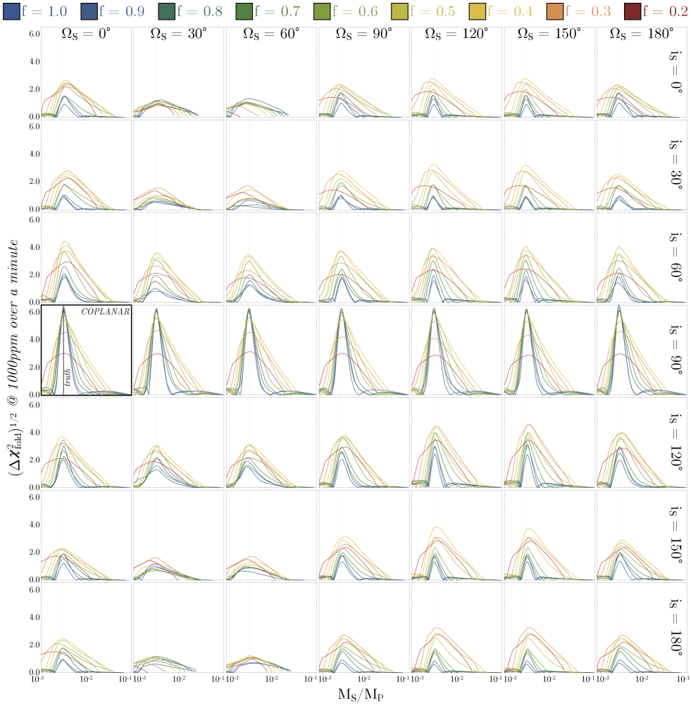
Figure 3: A multi-panel figure showing the effect of various choices of $i_{S}$ (rows), $\Omega_{S}$ (columns) and $f$ (colours; see top) on the moon-folding grid search. Each panel depicts the absolute $\sqrt{\Delta\chi^{2}}$ between the moon box model and a flat-line, which consistently recovers a signal at the correct $M_{S}/M_{P}$ value of $0.00315$, with the exception of some close-in moons in extremely inclined orbits. The detectability of the moon decreases in inclined configurations since it simply transits less often (see Martin, Fabrycky, & Montet 2019).

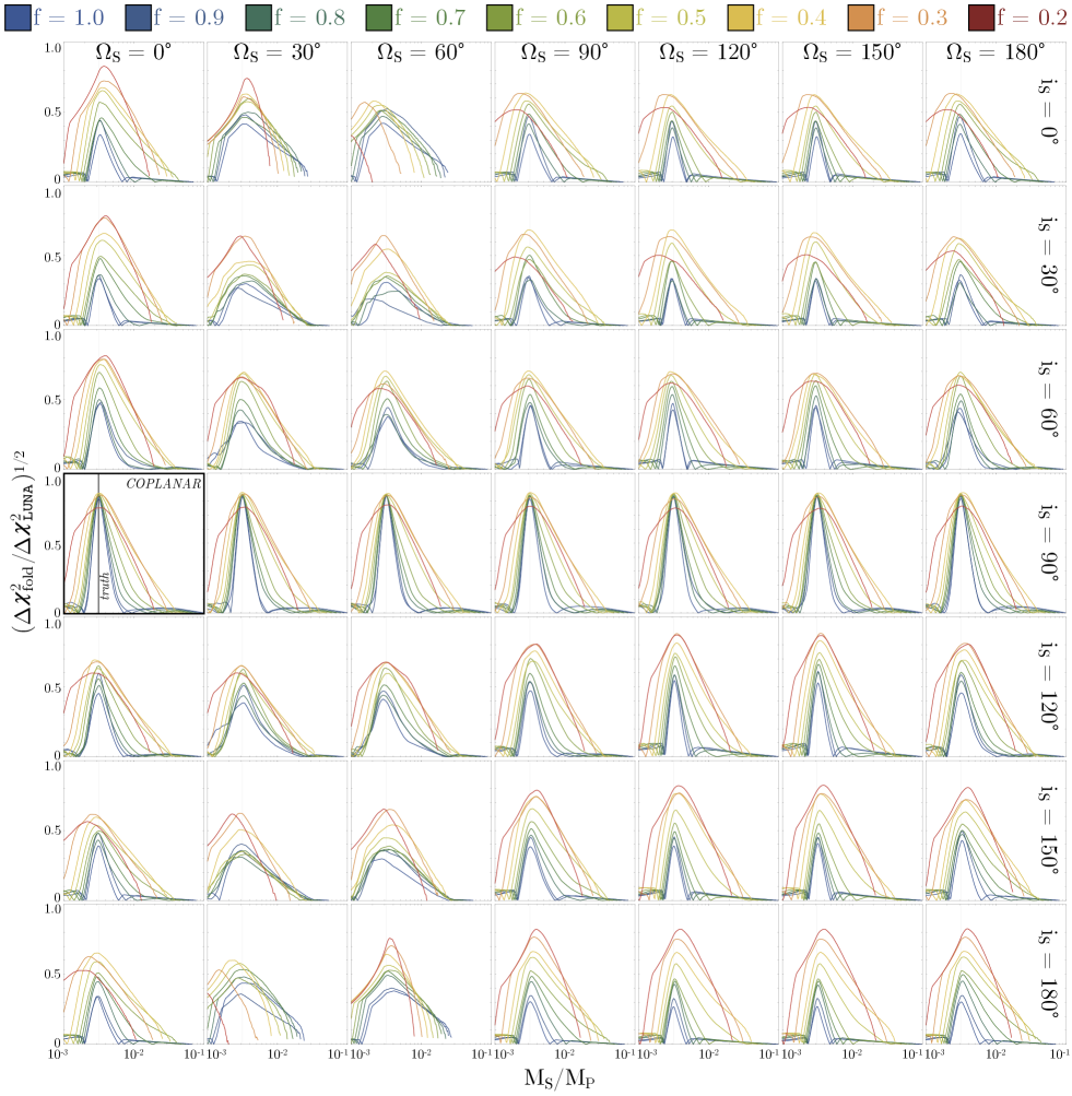
Figure 4: Same as Figure 3 except the change in $\chi^{2}$ is normalised to that produced when using the true photodynamic model used to generate the systems (LUNA). The moon-folding technique generally recovers over half of the available signal and for coplanar configurations it exceeds 80%.

4.3 Interpreting the simulated results

The first key result from this exercise is that in almost all cases the peak of the $M_{S}/M_{P}$ blind search centres on the expected true value, with the only exceptions being compact moons in nearly perpendicular geometries. On this basis, one should expect that the moon-folding technique will generally produce an accurate estimate of the most probable $M_{S}/M_{P}$ value for white noise dominated light curves.

The second key result is that the detectability of exomoons appears to diminish for inclined configurations, as shown in Figure 3. This is not surprising and simply a result of the lower duty cycles of such systems (Martin, Fabrycky, & Montet, 2019). This is also supported by the fact that Figure 4 shows far less attenuation of the inclined states, because even the photodynamic true signal is less detectable. This stems from the fact that inclined orbits will not necessarily transit each time and thus this will diminish the detectability of the stacked signal. In other words, in some of the stacked epochs, there is no dip to fold in. For coplanar moons, then, the moon-folding strategy produces a fully coherent signal, but for inclined states the signal can become “semi-coherent”.

The third key result is that, from Figure 4, the moon-folding technique recovers typically at least half of the available SNR but up to 80% for coplanar configurations. For a large moon which forms from the circumplanetary disk, such as Titan around Saturn, coplanar configurations are the natural outcome (Canup & Ward, 2002; Inderbitzi et al., 2020) and thus these should be well-recovered with this strategy.

Finally, it is noted that for coplanar configurations, wider moons are generally more detectable (by overlapping less often with the planet) and the moon-folding technique’s recovered signal, when compared to LUNA, is broadly independent of $f$. However, for inclined states, wide moons become less detectable because they have an increasingly large chance to not transit the star each epoch and thus evade detection (Martin, Fabrycky, & Montet, 2019). In a relative sense, the moon-folding approximation also becomes worse for such inclined moons because their paths deviate away the nominal $\hat{X}$-chord ever more.

5 Application to an Example System

5.1 Selection of Kepler-973b

As a final way of testing the new algorithm, a suitable Kepler transiting planet was sought as a real example case. A basic requirement of the new method is a planet which exhibits TTVs. Initially, Kepler-1625b might seem to be an ideal test case, given the known exomoon candidate there (Teachey & Kipping, 2018). However, with four transits, a linear ephemeris + sinusoid model is under-constrained (Kipping, 2021) and thus it is not possible to use the moon-folding method since one can’t make unique predictions for the satellite’s position. Looking further afield, TTVs are common within the Kepler catalog and so some thought on how to choose an appropriate system is required.

Following the aliasing theory presented in Kipping (2021), 90% of exomoons are expected to produce TTVs of periods between 2 to 20 cycles, and thus a known TTV system in this range was sought. Further, excessively large TTVs, or moderately large TTVs lacking associated TDVs, can be flagged as so-called “impossible moons” following the approach of Kipping & Teachey (2020).

With these filters in mind, let us take the Ofir et al. (2018) “spectral” TTV catalog as a starting point, which tabulates Kepler exoplanets exhibiting periodic TTVs to a false-alarm probability of $<1$%. From these, TTV periods $>20$ cycles were first filtered out (Kipping, 2021). Next, the surviving sample was cross-matched against those exoplanets identified in Kipping & Teachey (2020) that exhibit a periodic TTV at a statistical threshold of $\Delta(\mathrm{BIC})>10$ (using the Holczer et al. (2016) TTV catalog) and excludes any impossible moon cases.

Finally, the 24 cases were ranked by predicted $\mathrm{SNR}_{S}$ using Equation (20) and assuming a Ganymede-analog moon. This presented two Kepler planets with $\mathrm{SNR}_{S}(\mathrm{Ganymede})\sim 1$, noteably Kepler-858b ($\mathrm{SNR}_{S}(\mathrm{Ganymede})=1.1$) and Kepler-973b ($\mathrm{SNR}_{S}(\mathrm{Ganymede})=0.8$). Of the two, Kepler-973b exhibits a sinusoidal, moon-like TTV pattern, whereas Kepler-858b was more saw-tooth like. Accordingly, in this example, let us proceed with Kepler-973b, a $49.6$ d $2.1$ $R_{\oplus}$ single-planet system around a $K_{P}=13.2$ K3-dwarf.

5.2 Data processing

The long-cadence (no short-cadence was available) time series Kepler photometry was detrended using the method marginalised approach described in Teachey & Kipping (2018). The 28 transit epochs were split into three 10-9-9 groups which were fitted with a Mandel & Agol (2002) transit model allowing each epoch to have its own free transit time, $\tau_{i}$. This splitting reduces the total number of free parameters in each regression to a manageable size yet allows the transit shape constraint from other epochs to improve the obtainable precision in $\tau_{i}$ (see Teachey, Kipping, & Schmitt 2018 for the first example of this in action). A freely fitted quadratic $q_{1}$-$q_{2}$ limb darkening law was used (Kipping, 2013) throughout, with the quarter-to-quarter contamination values accounted for (Seager & Mallén-Ornelas, 2003), and numerical resampling was implemented on the long-cadences to account for integration time following the method of Kipping (2010). Regressions were performed using MultiNest (Feroz, Hobson, & Bridges, 2009).

The resulting transit times are shown in Figure 5, where the derived a-posteriori marginalised 1-$\sigma$ credible intervals (black) are compared with those reported in Holczer et al. (2016) (grey, dashed). In both cases, the maximum a-posteriori linear ephemeris (found from a separate global fit with no TTVs) has been subtracted. In addition, the panel below shows the resulting Lomb-Scargle periodogram. Ofir et al. (2018) report a TTV period of $17.1$ cycles, which is close to the best-fit solution in this work of $17.3$ cycles (amplitude 8.2 mins). The results presented here also agree with the Holczer et al. (2016) TTVs, but generally appear less susceptible to outlier measurements (likely as a result of the Bayesian segmenting procedure used; Teachey, Kipping, & Schmitt 2018).

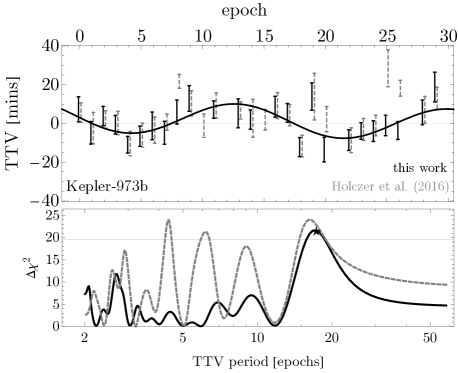
Figure 5: Top: TTVs of Kepler-973b derived in this work (black) versus those of Holczer et al. (2016) (gray, dashed). Overlaid is the best-fitting sinusoid to the TTV data of this work. Bottom: Lomb-Scargle periodograms of the above TTVs, where the horizontal line marks $\Delta(\mathrm{BIC})=10$.

5.3 Moon folding

Let us now proceed following the algorithm detailed in Section 2.3. In step 2b], one requires an input for $\mathrm{TTV}_{P}(t)$. In principle, this could be simply the TTV measurements directly, but given the sinusoidal nature of the TTVs (which is expected for an exomoon; see Equation 4), this works uses the best-fitting sinusoid determined in Section 5.2, (the black line plotted in the upper panel of Figure 5). To ensure no part of the real planetary transits leak into the predicted moon windows (which could cause a false-positive), both the measured and predicted locations of the planetary transits were excluded.

Using forecaster (Chen & Kipping, 2017) and the $R_{P}/R_{\star}$ posteriors, a posterior distribution for the planet-to-star mass-ratio, $q$, was inferred. This was then used with Equations (9) & (11) to define a $M_{S}/M_{P}$ grid from $0.0297$ to $0.748$. The next step was to scan along this grid at 100 log-uniformly separated intervals, which took 1 minute on a typical desktop computer. The results are summarised in Figure 6, where no significant moon-like dips were found. The highest significance solution occurs at around $M_{SP}=0.08$ yielding a $\sqrt{\Delta\chi^{2}}=2$ improvement - given the extra complexity of the moon model, such a modest improvement is not significant. Indeed, it is also noted that this region corresponds to an inverted moon transit of $(-42\pm 22)$ ppm and thus can be discounted as a possible moon (depicted in the inset of Figure 6’s upper panel).

Upper limits on the maximum positive moon dip were derived by simple $\chi^{2}$ perturbation, seeking a dip which increases the $\chi^{2}$ versus the null model of $+4$ (corresponding to 2 $\sigma$). This is shown by the hatched region of Figure 6’s lower panel. The right-hand axis converts these transit depths into physical radii by using the stellar radius, revealing that our observational limits probe down to 0.4 $R_{\oplus}$ - which is smaller than Ganymede.

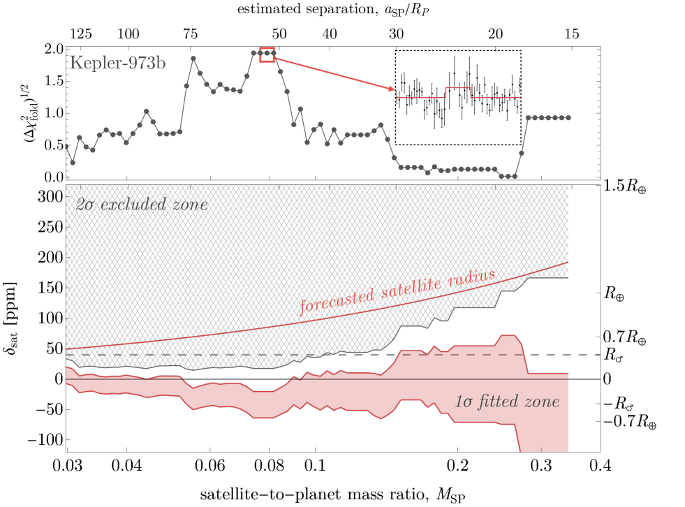
Figure 6: A real example of our moon-folding algorithm on Kepler-973b. Top panel shows the $\chi^{2}$ improvement of including a moon-dip versus $M_{SP}$, revealing no significant dips, with the largest dip being inverted (inset). Lower panel shows the corresponding transit depths (left-axis) and moon radii (right-axis), highlighting both the 1 $\sigma$ fitted region with solid shading and the excluded zone (hatched). Although no moon dips are found, our limits are sensitive down to Ganymede-sized moons.

Recall that a small $M_{SP}$ solution corresponds to a wider separated moon, since it is the product of these two that governs the measured TTV amplitude. In fact, one can estimate the corresponding exomoon semi-major axis in units of the planetary radius by re-arranging

$$A_{\mathrm{TTV-P}}=\frac{a_{SB}M_{SP}}{a_{P}n_{P}},$$

$$\Bigg{(}\frac{a_{SP}}{R_{P}}\Bigg{)}=A_{\mathrm{TTV-P}}\Bigg{(}\frac{M_{SP}}{1+M_{SP}}\Bigg{)}\Bigg{(}\frac{2\pi(a/R_{\star})}{P_{P}(R_{P}/R_{\star})}\Bigg{)},$$ (21)

which is used to populate the ticks on the upper $x$-axis of Figure 6, displaying a range from 15 to 125 planetary radii. Below 15 planetary radii, or equivalently above $M_{S}P>0.35$, the moon transits become so close to the planet that the number of points inside the folded moon signal is less than one datum. For this reason, even though a higher mass ratio is physically possible via Equation (9), our moon-folding approach is not sensitive to it.

Finally, it is noted that the $M_{SP}$ values on $x$-axis can be used to predict the expected physical size of such a moon. This was achieved by first forecasting the planetary mass (since no measurement currently exists) with forecaster, then multiplying this by the given $M_{SP}$ value to get a moon mass, and then forecasting back into radius space. This forecast is shown with the curved red line in the lower panel of Figure 6. Critically, this forecast is inside the observationally excluded zone across the entire range, meaning that the moon hypothesis can be fully excluded. In summary, one can use this technique to show that Kepler-973b’s TTVs are not being caused by a single moon.

6 Discussion

In this work, a new method has been proposed for performing a double fold of photometric time series of transiting planets in order to search for exomoons. In what follows, some of the limitations of this approach are discussed, as well possibles areas for improvement.

The method assumes a slow-moving moon, such that the moon’s transit duration is approximately equal to that of the planet. This is also an assumption built into the theory of TTVs due to exomoons(Kipping, 2011). Slow-moons also avoid the possibility of the moon conducting multiple half-orbits/transits during the planetary transit, which is not modelled. Further, fast-moons (those on compact orbits) are so close to the planet that the portion of the light curve where the moon is transiting but the planet is not is greatly diminished, minimising the available signal. We estimate a rigorous condition of $f\equiv(a_{S}/R_{H})\gg 3^{1/3}(M_{P}/M_{\star})^{2/3}$, and in practice expect the method to fail at $f\lesssim 0.1$. We also assume a coplanar moon orbit, but find the method still works for even highly inclined configurations but at reduced sensitivity - since the moon spends less time transiting the star (Martin, Fabrycky, & Montet, 2019).

An important limitation of the new method is that it only works if the exoplanet exhibits TTVs. The planetary TTV essentially resolves the moon’s aliased period and phase, leaving just the separation (although in practice the mass-ratio is used) as the remaining free parameter. In principle, one could imagine extending this method to non-TTV systems, but the grid search would necessarily become three-dimensional now, with the moon’s phase, period and separation all being unknown quantities. The latter two parameters could be combined into a single-term in the case where the planetary mass is precisely known, although this is somewhat complicated by the fact that methods such as radial velocities in fact measure the planet+satellite system combined mass. Nevertheless, this highlights the possibility of extending the transit origami approach to a broader population in future work.

In general, moon-folding will always be less sensitive than a full photodynamical model (Kipping, 2011). By culling the data inside the transit, approximating that the moon’s impact parameter is the same as that of the planet, and ignoring the acceleration effects of the moon’s orbit, the algorithm presented here cuts several corners in the name of efficiency. The true value of the approach here is to flag interesting signals, and it will still be necessary to perform more detailed tests and ensure physical orbital solutions exist (e.g. see Teachey & Kipping 2018).

An important step in the outlined algorithm is to first mask the known planetary transits and here a conservative approach is recommended, taking both the measured transits times and modelled TTV waveform as guides to ensure the transit is fully removed (as was done in the example application in Section 5). This is crucial to ensure that the wings of the planetary transit do not induce spurious moon-like signatures. As a result of this process though, close-in moons may get truncated. Yet more, standard exomoon TTV theory (and thus this method) breaks down for moons with periods comparable to the transit duration, which imposes an additional (but unrelated) barrier to detecting close-in moons. Together then, close-in moons will remain challenging with the outlined method. For example, in the case of Kepler-973b, it is not possible to probe interior to 15 planetary radii, which is the approximate position of Ganymede around Jupiter (i.e. a Callisto would be fine, but a Europa or Io is too close-in).

To conclude, it is highlighted that exomoons remains a vibrant intellectual topic. When it comes to detection, new approaches and methodological developments continue to arise by many teams, and enormous opportunities await the community when these are coupled to the rise of ever larger exoplanet surveys.

Data Availability

Data used in this paper is from the Kepler Space Telescope and can be found at the Mikulski Archive for Space Telescopes (MAST) which is hosted by the Space Telescope Science Institute (STScI). Additional data underlying the analysis was taken from the Holczer et al. (2016) catalogue, which is available on line. Notebooks used to generate the figures are made available at https://github.com/CoolWorlds/TransitOrigamiBits.

Software used: forecaster (Chen & Kipping, 2017), MultiNest (Feroz, Hobson, & Bridges, 2009), LUNA(Kipping, 2011), Mandel-Agol light curve model (Mandel & Agol, 2002).

References

- Akeson et al. (2013) Akeson R. L., Chen X., Ciardi D., Crane M., Good J., Harbut M., Jackson E., et al., 2013, PASP, 125, 989
- Ballard et al. (2014) Ballard S., Chaplin W. J., Charbonneau D., Désert J.-M., Fressin F., Zeng L., Werner M. W., et al., 2014, ApJ, 790, 12
- Barnes (2007) Barnes J. W., 2007, PASP, 119, 986
- Canup & Ward (2002) Canup R. M., Ward W. R., 2002, AJ, 124, 3404
- Carter et al. (2008) Carter J. A., Yee J. C., Eastman J., Gaudi B. S., Winn J. N., 2008, ApJ, 689, 499
- Charbonneau et al. (2000) Charbonneau D., Brown T. M., Latham D. W., Mayor M., 2000, ApJL, 529, L45
- Chen & Kipping (2017) Chen J. & Kipping D., 2017, ApJ, 834, 17
- Christiansen et al. (2012) Christiansen J. L., Jenkins J. M., Caldwell D. A., Burke C. J., Tenenbaum P., Seader S., Thompson S. E., et al., 2012, PASP, 124, 1279
- Cumming (2004) Cumming A., 2004, MNRAS, 354, 1165
- Dawson & Johnson (2012) Dawson R. I., Johnson J. A., 2012, ApJ, 756, 122
- Dulz & Reed (2017) Dulz S. & Reed M., 2017, AAS Meeting #229, id.245.13
- Feroz, Hobson, & Bridges (2009) Feroz F., Hobson M. P., Bridges M., 2009, MNRAS, 398, 1601
- Gillon et al. (2017) Gillon M., Triaud A. H. M. J., Demory B.-O., Jehin E., Agol E., Deck K. M., Lederer S. M., et al., 2017, Natur, 542, 456
- Gregory (2007) Gregory P. C., 2007, MNRAS, 374, 1321
- Hamers & Portegies Zwart (2018) Hamers A. S., Portegies Zwart S. F., 2018, ApJL, 869, L27
- Heller (2014) Heller R., 2014, ApJ, 787, 14
- Henry et al. (2000) Henry G. W., Marcy G. W., Butler R. P., Vogt S. S., 2000, ApJL, 529, L41
- Hippke (2015) Hippke M., 2015, ApJ, 806, 51
- Hippke & Heller (2019) Hippke M., Heller R., 2019, A&A, 623, A39
- Holczer et al. (2016) Holczer T., Mazeh T., Nachmani G., Jontof-Hutter D., Ford E. B., Fabrycky D., Ragozzine D., et al., 2016, ApJS, 225, 9
- Inderbitzi et al. (2020) Inderbitzi C., Szulágyi J., Cilibrasi M., Mayer L., 2020, MNRAS, 499, 1023
- Kane et al. (2012) Kane S. R., Ciardi D. R., Gelino D. M., von Braun K., 2012, MNRAS, 425, 757
- Kane (2017) Kane S. R., 2017, ApJL, 839, L19
- Kipping (2009a) Kipping, D. M., 2009a, MNRAS, 392, 181
- Kipping (2010) Kipping D. M., 2010, MNRAS, 408, 1758
- Kipping (2011) Kipping D. M., 2011a, MNRAS, 416, 689
- Kipping (2011) Kipping, D. M., 2011b, Ph.D. Thesis, University College London
- Kipping et al. (2012) Kipping D. M., Dunn W. R., Jasinski J. M., Manthri V. P., 2012, MNRAS, 421, 1166
- Kipping (2013) Kipping D. M., 2013, MNRAS, 435, 2152
- Kipping et al. (2014) Kipping D. M., Nesvorný D., Buchhave L. A., Hartman J., Bakos G. Á., Schmitt A. R., 2014, ApJ, 784, 28
- Kipping & Teachey (2020) Kipping D., Teachey A., 2020, SerAJ, 201, 25
- Kipping (2021) Kipping D., 2021, MNRAS, 500, 1851
- Kovács, Zucker, & Mazeh (2002) Kovács G., Zucker S., Mazeh T., 2002, A&A, 391, 369
- Mandel & Agol (2002) Mandel K., Agol E., 2002, ApJL, 580, L171
- Martin, Fabrycky, & Montet (2019) Martin D. V., Fabrycky D. C., Montet B. T., 2019, ApJL, 875, L25
- Muirhead et al. (2012) Muirhead P. S., Johnson J. A., Apps K., Carter J. A., Morton T. D., Fabrycky D. C., Pineda J. S., et al., 2012, ApJ, 747, 144
- Ofir et al. (2018) Ofir A., Xie J.-W., Jiang C.-F., Sari R., Aharonson O., 2018, ApJS, 234, 9
- Porter & Grundy (2011) Porter S. B., Grundy W. M., 2011, ApJL, 736, L14
- Sartoretti & Schneider (1999) Sartoretti, P. & Schneider, J., 1999, A&AS, 14, 550
- Seager & Mallén-Ornelas (2003) Seager S., Mallén-Ornelas G., 2003, ApJ, 585, 1038
- Simon et al. (2012) Simon A. E., Szabó G. M., Kiss L. L., Szatmáry K., 2012, MNRAS, 419, 164
- Teachey, Kipping, & Schmitt (2018) Teachey A., Kipping D. M., Schmitt A. R., 2018, AJ, 155, 36
- Teachey & Kipping (2018) Teachey A., Kipping D. M., 2018, SciA, 4, eaav1784
- Van Eylen et al. (2019) Van Eylen V., Albrecht S., Huang X., MacDonald M. G., Dawson R. I., Cai M. X., Foreman-Mackey D., et al., 2019, AJ, 157, 61
- Wang et al. (2013) Wang J., Fischer D. A., Barclay T., Boyajian T. S., Crepp J. R., Schwamb M. E., Lintott C., et al., 2013, ApJ, 776, 10
- Xie et al. (2016) Xie J.-W., Dong S., Zhu Z., Huber D., Zheng Z., De Cat P., Fu J., et al., 2016, PNAS, 113, 11431
- Zechmeister & Kürster (2009) Zechmeister M., Kürster M., 2009, A&A, 496, 577