Magnonic thermal transport using the quantum Boltzmann equation

Abstract

We present a formula for thermal transport in the bulk of Bose systems based on the quantum Boltzmann equation (QBE). First, starting from the quantum kinetic equation and using the Born approximation for impurity scattering, we derive the QBE of Bose systems and provide a formula for thermal transport subjected to a temperature gradient. Next, we apply the formula to magnons. Assuming a relaxation time approximation and focusing on the linear response regime, we show that the longitudinal thermal conductivity of the QBE exhibits the different behavior from the conventional. The thermal conductivity of the QBE reduces to the Drude-type in the limit of the quasiparticle approximation, while not in the absence of the approximation. Finally, applying the quasiparticle approximation to the QBE, we find that the correction to the conventional Boltzmann equation is integrated as the self-energy into the spectral function of the QBE, and this enhances the thermal conductivity. Thus we shed light on the thermal transport property of the QBE beyond the conventional.

I Introduction

The last decade has seen a rapid development of magnon-based spintronics, dubbed magnonics, aiming at utilizing the quantized spin waves, magnons, as a carrier of information Chumak et al. (2015). The main subject is the realization of efficient transmission of information using spins in insulating magnets. For this purpose, taking into account the fundamental difference of the quantum-statistical properties between electrons and magnons, i.e., fermions and bosons, respectively, many magnonic analogues of electron transport have been established both theoretically and experimentally Nakata et al. (2017a), with a particular focus on thermal transport, e.g., the thermal Hall effect Onose et al. (2010); Katsura et al. (2010); Matsumoto and Murakami (2011a, b) and the Wiedemann-Franz law Nakata et al. (2015, 2017b, 2017c, 2019a) for magnon transport.

The key ingredient in the study of thermal transport phenomena is the Boltzmann equation Ashcroft and Mermin (1976). As well as electron transport, the conventional Boltzmann equation has been playing a central role in the study of magnon transport, e.g., see Refs. Rezende et al. (2014a, b); Basso et al. (2016a, b, c); Okuma et al. (2017); Schmidt et al. (2018); Nakata et al. (2019b); Liu et al. (2019); Jiang et al. (2013); the temperature gradient ${\mathbf{\nabla}}T$ drives a magnonic system out of equilibrium. The conventional Boltzmann equation describes the property of the system at time $t$ as

$$\Big{(} \frac{\partial}{\partial t}+{\mathbf{v}}_{\mathbf{k}}\cdot{\mathbf{\nabla}}T\frac{\partial}{\partial T}\Big{)}f_{{\mathbf{k}},{\mathbf{r}},t}=I_{{\mathbf{k}},{\mathbf{r}},t},$$ (1)

where ${\mathbf{v}}_{\mathbf{k}}:=\partial\omega_{\mathbf{k}}/(\partial{\mathbf{k}})$ is the magnon velocity for the energy dispersion relation $\hbar\omega_{\mathbf{k}}$ in the wavenumber space ${\mathbf{k}}$, $\hbar$ represents the Planck constant, $f_{{\mathbf{k}},{\mathbf{r}},t}$ is the nonequilibrium Bose distribution function of the absolute temperature $T$, and $I_{{\mathbf{k}},{\mathbf{r}},t}$ is the collision integral for a position ${\mathbf{r}}$. Within the relaxation time approximation, the longitudinal thermal conductivity of magnons in the bulk of magnets is proportional to the relaxation time Nakata et al. (2017c, 2019b); Jiang et al. (2013). Under some conditions, the relaxation time coincides with the lifetime of magnons, which is proportional to the inverse of the Gilbert damping constant $\alpha$ See . Thus the magnonic thermal conductivity of the conventional Boltzmann equation reduces to the Drude-type Dru as a function of $\alpha$ in that it is proportional to $1/\alpha$.

From the viewpoint of quantum field theory, the conventional Boltzmann equation [Eq. (1)] is derived from the quantum kinetic equation  by taking several approximations Mahan (2000); Haug and Jauho (2007); Kita (2010); Danielewicz (1984). Assuming that the variation of the center-of-mass coordinates is slow compared with that of the relative coordinates, Kadanoff and Baym Kadanoff and Baym (1962) applied an approximation, called the gradient expansion, to the quantum kinetic equation for the nonequilibrium Green’s function Keldysh (1965). The quantum kinetic equation of the lowest order gradient approximation becomes the quantum Boltzmann equation (QBE). The QBE describes the equation of motion for the lesser Green’s function. The spectral function is assumed to be the Dirac delta function in the quasiparticle approximation Mahan (2000); Haug and Jauho (2007); Kita (2010); Matsuo et al. (2017); Nakata et al. (2019b). In the limit of the quasiparticle approximation, the QBE reduces to the conventional Boltzmann equation [Eq. (1)] for the nonequilibrium distribution function of three variables $({\mathbf{k}},{\mathbf{r}},t)$.

This hierarchical structure of quantum field theory indicates that by relaxing some of the approximations, quantum-mechanical corrections to the conventional Boltzmann equation can be evaluated Haug and Jauho (2007). Such sound development has been made successfully as to electrons Kita (2010). The lifetime of electrons in metals subjected to a strong impurity potential becomes substantial, and the quasiparticle approximation is not applicable. To solve the issue, Prange and Kadanoff introduced an alternative approach Prange and Kadanoff (1964), which was developed for the application to superconductors and superfluids Eilenberger (1968); Serene and Rainer (1983); Larkin and Ovchinnikov (1975); Kita (2001), e.g., the Eilenberger equation Eilenberger (1968). However, those are for Fermi systems. Since the approach is based on the assumption that Kita (2010) there is a Fermi surface and the Fermi energy, the developed formula is not applicable to Bose systems, e.g., magnons. Thus, to the best of our knowledge Loss , as for magnons in the bulk of magnets, the thermal transport property beyond the conventional Boltzmann equation remains an open issue.

In this paper, we provide a solution to this fundamental challenge by starting from the quantum kinetic equation and developing the QBE for Bose systems. The purpose of any useful formalism is to provide a method for calculation of measurable quantities. First, using the QBE we develop a formula for thermal transport in the bulk of Bose systems, including the nonlinear response to the temperature gradient. Next, as a platform, we apply it to magnons. In the conventional spintronics study, the Landau-Lifshitz-Gilbert equation is playing the central role Tserkovnyak et al. (2005). To develop a relation with it, using the Gilbert damping constant we describe the spectral function of magnons, and study the longitudinal thermal conductivity of the QBE. Finally, by applying the quasiparticle approximation to the thermal conductivity of the QBE, we find the correction to the conventional Boltzmann equation and discuss thermal transport properties beyond the conventional.

We remark that the conventional Boltzmann equation Rezende et al. (2014a, b); Basso et al. (2016a, b, c); Okuma et al. (2017); Schmidt et al. (2018); Nakata et al. (2019b); Liu et al. (2019); Jiang et al. (2013), i.e., the transport theory based on the quasiparticle approximation, can not describe paramagnons in the bulk of paramagnets Mahan (2000). The quasiparticle approximation assumes that the spectrum has the form of the Dirac delta function. However, the spectrum of paramagnons is broad in general, and has a peak with a sufficient width of a nonzero value associated with the inverse of the finite lifetime Doniach (1967); Hertz (1976); Doubble et al. (2010); the spectrum can not be approximated by the Dirac delta function. Therefore, the conventional Boltzmann equation can not describe paramagnons. In this paper, we will also shed light on this issue.

This paper is organized as follows. In Sec. II starting from the quantum kinetic equation of the lowest order gradient approximation and using the Born approximation for impurity scattering, we derive the QBE for Bose systems. In Sec. III, first, using the QBE and assuming a steady state in terms of time, we provide a formula for thermal transport in the bulk of Bose systems subjected to a temperature gradient, including the nonlinear response. Next, we apply the formula to magnons in Sec. III.1. To develop a relation with the conventional spintronics study, we describe the spectral function of magnons in terms of the Gilbert damping constant. Then, assuming a relaxation time approximation and focusing on the linear response regime, we evaluate the longitudinal thermal conductivity of magnons in the bulk of magnets based on the QBE. Finally, in Sec. III.2 applying the quasiparticle approximation to the magnonic thermal conductivity of the QBE, we discuss the difference from the one of the conventional Boltzmann equation. Comparing also with the linear response theory, we comment on our formula in Sec. IV. We remark on open issues in Sec. V and give some conclusions in Sec. VI. Technical details are deferred to the Appendices.

II Quantum Boltzmann equation for Bose system

We consider a Bose system where the center-of-mass coordinates, the position and time in center-of-mass (${\mathbf{r}},t$), respectively, vary slowly compared to the relative coordinates. Up to the lowest order of the gradient expansion, the quantum kinetic equation Mahan (2000); Haug and Jauho (2007); Kita (2010); Danielewicz (1984) for the system reduces to

$$-i\Big{(} \frac{\partial{\mathscr{H}}_{{\mathbf{k}},\omega}}{\partial t}\frac{\partial}{\partial\omega}-\frac{\partial{\mathscr{H}}_{{\mathbf{k}},\omega}}{\partial\omega}\frac{\partial}{\partial t}-\frac{\partial{\mathscr{H}}_{{\mathbf{k}},\omega}}{\partial{\mathbf{r}}}\frac{\partial}{\partial{\mathbf{k}}}+\frac{\partial{\mathscr{H}}_{{\mathbf{k}},\omega}}{\partial{\mathbf{k}}}\frac{\partial}{\partial{\mathbf{r}}}\Big{)}G^{<}_{{\mathbf{k}},\omega,{\mathbf{r}},t}$$

$$= (G^{<}_{{\mathbf{k}},\omega,{\mathbf{r}},t}\Sigma^{>}_{{\mathbf{k}},\omega,{\mathbf{r}},t}-G^{>}_{{\mathbf{k}},\omega,{\mathbf{r}},t}\Sigma^{<}_{{\mathbf{k}},\omega,{\mathbf{r}},t}),$$ (2)

where ${\mathscr{H}}_{{\mathbf{k}},\omega}:=\hbar\omega-\hbar\omega_{\mathbf{k}}$ for a frequency $\omega$ and the functions, $G^{<(>)}_{{\mathbf{k}},\omega,{\mathbf{r}},t}$ and $\Sigma^{<(>)}_{{\mathbf{k}},\omega,{\mathbf{r}},t}$, are the lesser (greater) component of the bosonic nonequilibrium Green’s function and that of the self-energy, respectively; the variables $({\mathbf{k}},\omega)$ arise from the Fourier transform of the relative coordinates. Following Ref. Mahan (2000), we refer to Eq. (2) as the QBE. The QBE is the equation of motion for the lesser Green’s function $G^{<}_{{\mathbf{k}},\omega,{\mathbf{r}},t}$ and consists of four variables $({\mathbf{k}},\omega,{\mathbf{r}},t)$, while the conventional Boltzmann equation is for the nonequilibrium Bose distribution function $f_{{\mathbf{k}},{\mathbf{r}},t}$ and of three variables $({\mathbf{k}},{\mathbf{r}},t)$. The QBE in the limit of the quasiparticle approximation reduces to the conventional Boltzmann equation. In this paper we study thermal transport of the QBE for Bose systems, and find the properties beyond the conventional Boltzmann equation. Then, applying the quasiparticle approximation to the thermal conductivity of the QBE, we discuss the difference from the conventional.

Within the Born approximation, the self-energy due to impurity scattering of the impurity potential $V_{{\mathbf{k}},{\mathbf{k}}^{\prime}}$ is given as $\Sigma_{{\mathbf{k}},\omega,{\mathbf{r}},t}=\sum_{{\mathbf{k}}^{\prime}}G_{{\mathbf{k}}^{\prime},\omega,{\mathbf{r}},t}\mid V_{{\mathbf{k}},{\mathbf{k}}^{\prime}}\mid^{2}$. Assuming that the function ${\mathscr{H}}_{{\mathbf{k}},\omega}$ is time-independent and spatially uniform, the QBE becomes

$$( \partial_{t}+{\mathbf{v}}_{\mathbf{k}}\cdot\partial_{\mathbf{r}})G^{<}_{{\mathbf{k}},\omega,{\mathbf{r}},t}$$ (3)

$$= \frac{1}{i\hbar}\sum_{{\mathbf{k}}^{\prime}}\mid V_{{\mathbf{k}},{\mathbf{k}}^{\prime}}\mid^{2}(G^{<}_{{\mathbf{k}},\omega,{\mathbf{r}},t}G^{>}_{{\mathbf{k}}^{\prime},\omega,{\mathbf{r}},t}-G^{>}_{{\mathbf{k}},\omega,{\mathbf{r}},t}G^{<}_{{\mathbf{k}}^{\prime},\omega,{\mathbf{r}},t}).$$

The QBE consists of the lesser (greater) Green’s functions $G^{<(>)}_{{\mathbf{k}},\omega,{\mathbf{r}},t}$. The Kadanoff-Baym ansatz ensures that Mahan (2000); Haug and Jauho (2007); Kita (2010) the Green’s functions are associated with the spectral function ${\cal{A}}_{{\mathbf{k}},\omega,{\mathbf{r}},t}$ and the nonequilibrium distribution function $\phi_{{\mathbf{k}},\omega,{\mathbf{r}},t}$ as $G^{<}_{{\mathbf{k}},\omega,{\mathbf{r}},t}=-i{\cal{A}}_{{\mathbf{k}},\omega,{\mathbf{r}},t}\phi_{{\mathbf{k}},\omega,{\mathbf{r}},t}$ and $G^{>}_{{\mathbf{k}},\omega,{\mathbf{r}},t}=-i{\cal{A}}_{{\mathbf{k}},\omega,{\mathbf{r}},t}(1+\phi_{{\mathbf{k}},\omega,{\mathbf{r}},t})$ for bosons, while $G^{<}_{{\mathbf{k}},\omega,{\mathbf{r}},t}=i{\cal{A}}_{{\mathbf{k}},\omega,{\mathbf{r}},t}\phi_{{\mathbf{k}},\omega,{\mathbf{r}},t}$ and $G^{>}_{{\mathbf{k}},\omega,{\mathbf{r}},t}=-i{\cal{A}}_{{\mathbf{k}},\omega,{\mathbf{r}},t}(1-\phi_{{\mathbf{k}},\omega,{\mathbf{r}},t})$ for fermions. The nonequilibrium Bose distribution function in the wavenumber space is given as $f_{{\mathbf{k}},{\mathbf{r}},t}^{\textrm{QBE}}:=\int[\hbar d\omega/(2\pi)]{\cal{A}}_{{\mathbf{k}},\omega,{\mathbf{r}},t}\phi_{{\mathbf{k}},\omega,{\mathbf{r}},t}$. Using the Kadanoff-Baym ansatz for bosons, finally, we obtain the QBE of the functions ${\cal{A}}_{{\mathbf{k}},\omega,{\mathbf{r}},t}$ and $\phi_{{\mathbf{k}},\omega,{\mathbf{r}},t}$ as

$$( \partial_{t}+{\mathbf{v}}_{\mathbf{k}}\cdot\partial_{\mathbf{r}})({\cal{A}}_{{\mathbf{k}},\omega,{\mathbf{r}},t}\phi_{{\mathbf{k}},\omega,{\mathbf{r}},t})$$ (4)

$$=- \frac{1}{\hbar}\sum_{{\mathbf{k}}^{\prime}}\mid V_{{\mathbf{k}},{\mathbf{k}}^{\prime}}\mid^{2}{\cal{A}}_{{\mathbf{k}},\omega,{\mathbf{r}},t}{\cal{A}}_{{\mathbf{k}}^{\prime},\omega,{\mathbf{r}},t}(\phi_{{\mathbf{k}},\omega,{\mathbf{r}},t}-\phi_{{\mathbf{k}}^{\prime},\omega,{\mathbf{r}},t}).$$

The QBE is useful to a wide range of Bose system subjected to impurity scattering. For convenience, we define the collision integral as ${\cal{I}}_{{\mathbf{k}},\omega,{\mathbf{r}},t}:=-\sum_{{\mathbf{k}}^{\prime}}\mid V_{{\mathbf{k}},{\mathbf{k}}^{\prime}}\mid^{2}{\cal{A}}_{{\mathbf{k}},\omega,{\mathbf{r}},t}{\cal{A}}_{{\mathbf{k}}^{\prime},\omega,{\mathbf{r}},t}(\phi_{{\mathbf{k}},\omega,{\mathbf{r}},t}-\phi_{{\mathbf{k}}^{\prime},\omega,{\mathbf{r}},t})/\hbar$. Hereafter, for simplicity, we drop the indices (${\mathbf{r}},t$) when those are not important.

III Thermal transport in
Bose system

The temperature gradient drives the Bose system out of equilibrium and generate a heat current. The QBE [Eq. (4)] describes the transport property of a steady state in terms of time as

$${\mathbf{v}}_{\mathbf{k}}\cdot{\mathbf{\nabla}}T\frac{\partial}{\partial T}({\cal{A}}_{{\mathbf{k}},\omega}\phi_{{\mathbf{k}},\omega})={\cal{I}}_{{\mathbf{k}},\omega},$$ (5)

where we assume that the temperature gradient is spatially uniform ${\mathbf{\nabla}}T=({\textrm{const.}})$. In this section, first, using the functions ${\cal{A}}_{{\mathbf{k}},\omega}$ and $\phi_{{\mathbf{k}},\omega}$ of the QBE [Eq. (5)], we provide a formula for the heat current in the bulk of two-dimensional Bose systems. Next, as a platform, in Sec. III.1 we apply the formula to magnons in two-dimensional insulating magnets. Assuming a relaxation time approximation for the function ${\cal{A}}_{{\mathbf{k}},\omega}\phi_{{\mathbf{k}},\omega}$ and focusing on the linear response regime, we evaluate the thermal conductivity in the bulk of the magnet. Finally, in Sec. III.2 applying the quasiparticle approximation to the magnonic thermal conductivity of the QBE, we discuss the difference from the one of the conventional Boltzmann equation.

The applied temperature gradient drives the system out of equilibrium and the Bose distribution function $\phi_{{\mathbf{k}},\omega}$ deviates from the one $\phi_{0}=({\text{e}}^{\beta\hbar\omega}-1)^{-1}$ in equilibrium, where $\beta:=1/(k_{\textrm{B}}T)$ is the inverse temperature and $k_{\textrm{B}}$ represents the Boltzmann constant. The deviation is characterized as the function $\delta\phi_{{\mathbf{k}},\omega}:=\phi_{{\mathbf{k}},\omega}-\phi_{0}$. Since the self-energy arises from impurity scattering, we assume that the spectral function ${\cal{A}}_{{\mathbf{k}},\omega}$ is little influenced by temperature and neglect the temperature dependence. Therefore the nonequilibrium Bose distribution function in the wavenumber space is given as $f_{\mathbf{k}}^{\textrm{QBE}}=f_{0}^{\textrm{QBE}}+\delta f_{\mathbf{k}}^{\textrm{QBE}}$ with $f_{0}^{\textrm{QBE}}:=\int[\hbar d\omega/(2\pi)]{\cal{A}}_{{\mathbf{k}},\omega}\phi_{0}$ and $\delta f_{\mathbf{k}}^{\textrm{QBE}}:=\int[\hbar d\omega/(2\pi)]{\cal{A}}_{{\mathbf{k}},\omega}\delta\phi_{{\mathbf{k}},\omega}$. The function consists of two parts; the equilibrium component $f_{0}^{\textrm{QBE}}$ and the nonequilibrium one $\delta f_{\mathbf{k}}^{\textrm{QBE}}$. Since each mode $\omega$ subjected to a chemical potential $\mu$ carries the energy $\hbar\omega$, the heat current density in the bulk of two-dimensional Bose systems, ${\mathbf{j}}_{Q}=(j_{Q_{x}},j_{Q_{y}})$, is given as

$${\mathbf{j}}_{Q}=\int\frac{d^{2}{\mathbf{k}}}{(2\pi)^{2}}{\mathbf{v}}_{\mathbf{k}}\int\frac{\hbar d\omega}{2\pi}(\hbar\omega-\mu){\cal{A}}_{{\mathbf{k}},\omega}\delta\phi_{{\mathbf{k}},\omega}.$$ (6)

This is the formula for the heat current density of the QBE, including the nonlinear response to the temperature gradient. The formula [Eq. (6)] is useful to Bose systems (e.g., insulators and metals) with the spectral function of arbitrary shape.

III.1 Magnonic thermal conductivity

As a platform, we apply the formula for the heat current of the QBE [Eq. (6)] to magnons in a two-dimensional insulating magnet where time-reversal symmetry is broken, e.g., due to an external magnetic field. At sufficiently low temperatures, the effect of magnon-magnon interactions and that of phonons are negligibly small, and impurity scattering makes a major contribution to the self-energy. Therefore, we work under the assumption that the spectral function ${\cal{A}}_{{\mathbf{k}},\omega}$ is little influenced by temperature, and neglect the temperature dependence.

First, we comment on the chemical potential of magnons subjected to the temperature gradient  Nakata et al. (2015, 2017b, 2017c). The applied temperature gradient induces magnon transport, which leads to an accumulation of magnons at the boundaries and builds up a nonuniform magnetization in the sample. This magnetization gradient plays a role of an effective magnetic field gradient and works as the gradient of a nonequilibrium spin chemical potential Basso et al. (2016b); Cornelissen et al. (2016); Du et al. (2017); Demokritov et al. (2006) for magnons. This generates a counter-current of magnons and thus the nonequilibrium spin chemical potential contributes to the thermal conductivity. See Ref. Nakata et al. (2017c) for details. In this paper, for simplicity, we consider a sufficiently large system and work under the assumption that the effect of the boundaries is negligibly small. Consequently, the nonequilibrium magnon accumulation becomes negligible and the nonequilibrium spin chemical potential of magnons vanishes. In the magnonic system, the heat current is identified with the energy current Matsumoto and Murakami (2011a); Nakata et al. (2017b). Note that Basso et al. (2016b); Cornelissen et al. (2016); Du et al. (2017); Demokritov et al. (2006) the spin chemical potential of magnons is peculiar to the system out of equilibrium .

Then, we consider thermal transport carried by magnons with the energy dispersion relation $\hbar\omega_{\mathbf{k}}=Dk^{2}+\Delta$, where $D$ represents the spin stiffness constant, $k:=|{\mathbf{k}}|$ denotes the magnitude of the wavenumber, and $\Delta$ is the magnon energy gap, e.g., due to an external magnetic field and a spin anisotropy, etc. Assuming a relaxation time approximation for the function ${\cal{A}}_{{\mathbf{k}},\omega}\phi_{{\mathbf{k}},\omega}$ of

$${\cal{I}}_{{\mathbf{k}},\omega}=-\frac{{\cal{A}}_{{\mathbf{k}},\omega}\phi_{{\mathbf{k}},\omega}-{\cal{A}}_{{\mathbf{k}},\omega}\phi_{0}}{\tau_{{\mathbf{k}},\omega}^{\textrm{R}}}$$ (7)

and focusing on the linear response regime, from Eq. (5) the nonequilibrium component $\delta\phi_{{\mathbf{k}},\omega}$ is given as

$$\delta\phi_{{\mathbf{k}},\omega}=-\tau_{{\mathbf{k}},\omega}^{\textrm{R}}{\mathbf{v}}_{\mathbf{k}}\cdot{\mathbf{\nabla}}T\frac{\partial\phi_{0}}{\partial T}+O(({\mathbf{\nabla}}T)^{2}),$$ (8)

where $\tau_{{\mathbf{k}},\omega}^{\textrm{R}}$ is the relaxation time for the magnonic system. Under the assumption that impurity scattering is elastic and that the relaxation time depends solely on the magnitude of the wavenumber, it is evaluated as ${1}/{\tau_{{\mathbf{k}},\omega}^{\textrm{R}}}=\sum_{{\mathbf{k}}^{\prime}}\mid V_{{\mathbf{k}},{\mathbf{k}}^{\prime}}\mid^{2}{\cal{A}}_{{\mathbf{k}}^{\prime},\omega}(1-{{\mathbf{v}}_{\mathbf{k}}\cdot{\mathbf{v}}_{{\mathbf{k}^{\prime}}}}/{\mid{\mathbf{v}}_{\mathbf{k}}\mid^{2}})/\hbar$. We remark that the relaxation time $\tau_{{\mathbf{k}},\omega}^{\textrm{R}}$ is different from the magnon lifetime $\tau_{{\mathbf{k}},\omega}^{\textrm{L}}$ in general. Those are distinct quantities. However, when the impurity potential is localized in space, the Fourier component $V_{{\mathbf{k}},{\mathbf{k}}^{\prime}}$ becomes independent of the wavenumber, and the relaxation time coincides with the magnon lifetime, which takes a wavenumber-independent value as $\tau_{\omega}^{\textrm{R}}=\tau_{\omega}^{\textrm{L}}$. From the Landau-Lifshitz-Gilbert equation Tserkovnyak et al. (2005), the magnon lifetime is associated with the inverse of the Gilbert damping constant $\alpha$ and it is described as Adachi et al. (2011); Ohnuma et al. (2014); Abrikosov et al. (1975); Tatara (2015a); Kovalev and Tserkovnyak (2012); Jiang et al. (2013) $\hbar/(2\tau_{\omega}^{\textrm{L}})=\alpha\hbar\omega$. Therefore, under the assumption that the real part of the self-energy is negligibly small compared with the magnon energy gap, the spectral function is given as ${\cal{A}}_{{\mathbf{k}},\omega}=2\alpha\hbar\omega/[({\mathscr{H}}_{{\mathbf{k}},\omega})^{2}+(\alpha\hbar\omega)^{2}]$. See Appendices for details See .

Finally, from Eqs. (6) and (8), we obtain the longitudinal thermal conductivity of magnons in the bulk of the two-dimensional insulating magnet, $\kappa_{xx}:=-j_{Q_{x}}/(\partial_{x}T)$, as

$$\kappa_{xx}= \frac{1}{2}\Big{(}\frac{D}{\pi}\Big{)}^{2}\frac{1}{k_{\textrm{B}}T^{2}}\int_{0}^{\infty}dkk^{3}$$

$$\cdot \int d\omega\frac{(\hbar\omega)^{2}}{({\mathscr{H}}_{{\mathbf{k}},\omega})^{2}+(\alpha\hbar\omega)^{2}}\frac{{\textrm{e}}^{\beta\hbar\omega}}{({\textrm{e}}^{\beta\hbar\omega}-1)^{2}},$$ (9)

where we assume that the temperature gradient is applied along the $x$ axis. In contrast to the conventional Boltzmann equation (cf., Sec. I), the thermal conductivity of the QBE in the absence of the quasiparticle approximation does not reduce to the Drude-type Dru , as a function of the Gilbert damping constant $\alpha$, in that it is not proportional to $1/\alpha$. The factor $1/\alpha$ arises from the relaxation time $\tau_{\omega}^{\textrm{R}}$ in $\delta\phi_{{\mathbf{k}},\omega}$ [Eq. (8)] as $\tau_{\omega}^{\textrm{R}}=\tau_{\omega}^{\textrm{L}}={1}/(2\alpha\omega)$. However, it cancels out by the factor $2\alpha\hbar\omega$ of the spectral function ${\cal{A}}_{{\mathbf{k}},\omega}=2\alpha\hbar\omega/[({\mathscr{H}}_{{\mathbf{k}},\omega})^{2}+(\alpha\hbar\omega)^{2}]$ [Eq. (6)]. Therefore the integrand remains the Lorentz-type , and the thermal conductivity of the QBE does not reduce to the Drude-type in the absence of the quasiparticle approximation.

III.2 Comparison: Conventional Boltzmann equation

The QBE in the limit of the quasiparticle approximation reduces to the conventional Boltzmann equation, which provides the thermal conductivity of the Drude-type Dru in terms of the Gilbert damping constant $\alpha$ (cf., Sec. I). This agrees with our formula of the QBE [Eq. (6)]; when we employ the quasiparticle (qp) approximation ${\cal{A}}_{{\mathbf{k}},\omega}\approx{\cal{A}}_{{\mathbf{k}},\omega}^{\textrm{qp}}:=2\pi\delta({\mathscr{H}}_{{\mathbf{k}},\omega})$ for Eq. (6), the thermal conductivity of the QBE reduces to $\kappa_{xx}\approx\kappa_{xx}^{\textrm{qp}}$ as

$$\kappa_{xx}^{\textrm{qp}}=\frac{1}{2}\Big{(}\frac{D}{\pi}\Big{)}^{2}\frac{1}{k_{\textrm{B}}T^{2}}\frac{\pi}{\alpha}\int_{0}^{\infty}dkk^{3}\omega_{\mathbf{k}}\frac{{\textrm{e}}^{\beta\hbar\omega_{\mathbf{k}}}}{({\textrm{e}}^{\beta\hbar\omega_{\mathbf{k}}}-1)^{2}}.$$ (10)

This is consistent with Eq. (9) in the limit of $\alpha\rightarrow 0$. Thus we find in the limit of the quasiparticle approximation that the thermal conductivity of the QBE becomes the Drude-type, as a function of $\alpha$, in that it is proportional to $1/\alpha$ as $\kappa_{xx}\approx\kappa_{xx}^{\textrm{qp}}\propto{1}/{\alpha}$. The factor $1/\alpha$ arises from the relaxation time $\tau_{\omega}^{\textrm{R}}=\tau_{\omega}^{\textrm{L}}={1}/(2\alpha\omega)$ in $\delta\phi_{{\mathbf{k}},\omega}$ [Eq. (8)].

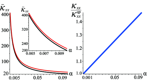
Figure 1: (Left) Plots of the rescaled thermal conductivity of magnons, ${\tilde{\kappa}}_{xx}:=[2\pi^{2}\hbar/(k_{\textrm{B}}^{2}T)]{\kappa}_{xx}$, as a function of the Gilbert damping constant $\alpha$  Heinrich et al. (2011); Tserkovnyak et al. (2002) obtained by numerically solving Eqs. (9) and  (10) for $\Delta=k_{\textrm{B}}T$ with a fixed temperature. Red line: Eq. (9) of the QBE. Black line: Eq. (10) for $\kappa_{xx}\approx\kappa_{xx}^{\textrm{qp}}$ in the limit of the quasiparticle approximation, i.e., the conventional Boltzmann equation. The correction to the conventional Boltzmann equation enhances the thermal conductivity. Inset: The enhancement still works and remains significant even for small values of the parameter $\alpha$. (Right) The plot of the ratio, $\kappa_{xx}/\kappa_{xx}^{\textrm{qp}}=1+(\kappa_{xx}-\kappa_{xx}^{\textrm{qp}})/\kappa_{xx}^{\textrm{qp}}$, as a function of the Gilbert damping constant $\alpha$, i.e., the ratio of the magnonic thermal conductivity $\kappa_{xx}$ of the QBE to the one $\kappa_{xx}^{\textrm{qp}}$ of the conventional Boltzmann equation (i.e., the QBE in the limit of the quasiparticle approximation). In units of $\kappa_{xx}^{\textrm{qp}}$, the correction to the conventional one and the resulting enhancement of the magnonic thermal conductivity increase as the value of $\alpha$ becomes large.

In conclusion, using the QBE we have developed the formula for thermal transport in the bulk of Bose systems, with a particular focus on magnons. As a function of the Gilbert damping constant, the thermal conductivity of the QBE reduces to the Drude-type Dru in the limit of the quasiparticle approximation, while not in the absence of the approximation. This is the main difference in the thermal conductivity between the QBE and the conventional one.

We remark that our formula based on the QBE reduces to the Drude-type Dru in the limit of the quasiparticle approximation. This means that, by relaxing the quasiparticle approximation, the correction to the conventional Boltzmann equation is integrated as the self-energy into the spectral function ${\cal{A}}_{{\mathbf{k}},\omega,{\mathbf{r}},t}$ of the QBE; Fig. 1 shows that the correction to the conventional Boltzmann equation enhances the thermal conductivity of the QBE. Thus our thermal transport theory of the QBE with four variables $({\mathbf{k}},\omega,{\mathbf{r}},t)$ is identified as an appropriate extension of the one of the conventional Boltzmann equation with three variables $({\mathbf{k}},{\mathbf{r}},t)$.

IV Discussion

To conclude a few comments on our approach are in order. First, the conventional Boltzmann equation Rezende et al. (2014a, b); Basso et al. (2016a, b, c); Okuma et al. (2017); Schmidt et al. (2018); Nakata et al. (2019b); Liu et al. (2019); Jiang et al. (2013) [Eq. (1)], i.e., the transport theory based on the quasiparticle approximation, can not describe paramagnons Mahan (2000). The quasiparticle approximation assumes that the spectrum has the form of the Dirac delta function. However, the spectrum of paramagnons is broad in general, and has a peak with a sufficient width of a nonzero value associated with the inverse of the finite lifetime Doniach (1967); Hertz (1976); Doubble et al. (2010); the spectrum of paramagnons can not be approximated by the Dirac delta function. Therefore, the conventional Boltzmann equation can not describe paramagnons. On the other hand, our formula based on the QBE is applicable to magnons with the spectrum of arbitrary shape [Eq. (6)]. In that sense, it is expected that our thermal transport theory is useful also to paramagnons in the bulk of paramagnets .

We remark that as well as insulators, our formula [Eq. (6)] is applicable, in principle, also to metals; the spectral function is described in terms of the Gilbert damping constant See , and the value for metals (e.g., transition metal ferromagnets) Bhagat and Lubitz (1974) $\alpha=O(10^{-2})$ is large compared with that for insulators $\alpha=O(10^{-3})$ in general Tserkovnyak et al. (2005); Heinrich et al. (2011); Tserkovnyak et al. (2002). Fig. 1 shows the behavior of the magnonic thermal conductivity in the region $O(10^{-3})\leq\alpha\leq O(10^{-2})$. As seen in the right of Fig. 1, $\kappa_{xx}/\kappa_{xx}^{\textrm{qp}}=1+(\kappa_{xx}-\kappa_{xx}^{\textrm{qp}})/\kappa_{xx}^{\textrm{qp}}$, in units of $\kappa_{xx}^{\textrm{qp}}$ the correction to the conventional Boltzmann equation and the resulting enhancement of the magnonic thermal conductivity increase as the value of $\alpha$ becomes large. The damping constant is associated with the inverse of the magnon lifetime See .

Next, our formula based on the QBE has an advantage over the linear response theory that it includes the nonlinear response; Eq. (6) is the formula for the heat current density including the nonlinear response to the temperature gradient. Here, using the QBE we develop an analysis on the nonlinear response. We apply the relaxation time approximation [Eq. (7)] for the function ${\cal{A}}_{{\mathbf{k}},\omega}\phi_{{\mathbf{k}},\omega}$ to the QBE [Eq. (5)]. Since the relaxation is induced by impurity scattering, we assume that the relaxation time is little influenced by temperature, and neglect the temperature dependence. Using the method of successive substitution, the nonequilibrium component of the Bose distribution function $\delta\phi_{{\mathbf{k}},\omega}$ [Eq. (6)] is evaluated, beyond the liner response regime, as $\delta\phi_{{\mathbf{k}},\omega}=\sum_{n=1}^{\infty}(-\tau_{{\mathbf{k}},\omega}^{\textrm{R}}{\mathbf{v}}_{\mathbf{k}}\cdot{\mathbf{\nabla}}T)^{n}[{\partial^{n}\phi_{0}}/({\partial T^{n}})]$, where the nonequilibrium component $\delta\phi_{{\mathbf{k}},\omega}$ is arranged in terms of the function $({\mathbf{\nabla}}T)^{n}$. Lastly, combining this equation with Eq. (6), we can obtain each coefficient of the nonlinear response to the temperature gradient. The formula is not restricted to magnonic systems, and it is useful to a wide range of Bose systems.

Finally, we add a comment to the linear response theory. According to Ref. Tatara (2015a), which focuses on the region $\alpha\ll 1$, the linear response theory (i.e., Kubo formula) results in the magnonic thermal conductivity of the Drude-type Dru , the same as the conventional Boltzmann equation, in that it is proportional to the inverse of the Gilbert damping constant. Note that the temperature gradient is not mechanical force but thermodynamic force; the temperature gradient is not described by a microscopic Hamiltonian. Therefore it is not straightforward to integrate the temperature gradient into the linear response theory. Ref. Tatara (2015a) described the effect of the temperature gradient with the help of the thermal vector potential  Tatara (2015b) associated with the Luttinger’s approach Luttinger (1964). For the details, see Ref. Tatara (2015a). We remark that the Boltzmann equation has no difficulty in integrating the temperature gradient into the formalism, e.g., see Eq. (1).

V Outlook

We give a few perspectives on further research. As a platform, in Sec. III.1 and Sec. III.2 focusing on insulating magnets at sufficiently low temperature, we have studied thermal transport of magnons under the assumption that the effect of magnon-magnon interactions and that of phonons are negligibly small, and that elastic impurity scattering makes a major contribution to the self-energy. It is of interest to study those effects on magnonic thermal transport of the QBE, with considering also the case that impurity scattering is inelastic .

In this paper relaxing the quasiparticle approximation and using the QBE for Bose systems, we have found that the correction to the conventional Boltzmann equation enhances the thermal conductivity. Therefore, based on the QBE it is intriguing to study the effect of the correction on the magnonic Wiedemann-Franz law Nakata et al. (2015, 2017b, 2017c, 2019a); at low temperatures magnon transport obeys a magnonic analogue of the Wiedemann-Franz law Franz and Wiedemann (1853), a universal law, in that the ratio of heat to spin conductivity is linear in temperature and does not depend on material parameters except the $g$-factor. Note that the magnonic Wiedemann-Franz law for the bulk of magnets has been proposed in Ref. Nakata et al. (2017c) based on the conventional Boltzmann equation. For the magnonic Wiedemann-Franz law of the QBE, the spin conductivity and the off-diagonal elements of the Onsager coefficient Nakata et al. (2017c) remain to be obtained. We believe it can be evaluated by following the study Mahan (2000) on the electrical conductivity of the QBE and developing it into the Bose system. Using the QBE, it will be intriguing also to study the magnonic Hall coefficients in topologically nontrivial magnonic systems Katsura et al. (2010); Matsumoto and Murakami (2011a, b); Nakata et al. (2017b, c, 2019a).

VI Conclusion

Developing the quantum Boltzmann equation, we have provided the formula for thermal transport in the bulk of Bose systems, including the nonlinear response to the temperature gradient. We have then applied the formula to magnons and have shown that thermal transport of the quantum Boltzmann equation exhibits the different behavior from the conventional. The longitudinal thermal conductivity of the quantum Boltzmann equation reduces to the Drude-type in the limit of the quasiparticle approximation, while not in the absence of the approximation. Relaxing the quasiparticle approximation, we have found that the correction to the conventional Boltzmann equation is integrated as the self-energy into the spectral function of the quantum Boltzmann equation, and this enhances the thermal conductivity. Our formula is useful to Bose systems, including metals as well as insulators, with the spectral function of arbitrary shape. Using the quantum Boltzmann equation we have found the thermal transport property beyond the conventional.

Appendix A Relaxation time and magnon lifetime

In this Appendix, we show that the relaxation time coincides with the magnon lifetime and takes a wavenumber-independent value under the assumption that; the relaxation time depends solely on the magnitude of the wavenumber, impurity scattering is elastic, and the impurity potential is localized in space. We remark that at sufficiently low temperatures, the effect of magnon-magnon interactions and that of phonons are negligibly small, and impurity scattering makes a major contribution to the self-energy. Therefore, we assume that the spectral function is little influenced by temperature and neglect the temperature dependence.

We consider magnons with the energy dispersion relation of $\hbar\omega_{\mathbf{k}}=Dk^{2}+\Delta$, where $|{\mathbf{k}}|=:k$ denotes the magnitude of the wavenumber. First, assuming the steady state in terms of time and applying the relaxation time approximation for the function ${\cal{A}}_{{\mathbf{k}},\omega}\phi_{{\mathbf{k}},\omega}$ to the QBE (see the main text), within the linear response regime we obtain the nonequilibrium component $\delta\phi_{{\mathbf{k}},\omega}$ as $\delta\phi_{{\mathbf{k}},\omega}=-\tau_{{\mathbf{k}},\omega}^{\textrm{R}}{\mathbf{v}}_{\mathbf{k}}\cdot{\mathbf{\nabla}}T[\partial\phi_{0}/(\partial T)]+O(({\mathbf{\nabla}}T)^{2})$. Next, using the relaxation time approximation for the collision integral ${\cal{I}}_{{\mathbf{k}},\omega}=-\sum_{{\mathbf{k}}^{\prime}}\mid V_{{\mathbf{k}},{\mathbf{k}}^{\prime}}\mid^{2}{\cal{A}}_{{\mathbf{k}},\omega}{\cal{A}}_{{\mathbf{k}}^{\prime},\omega}(\phi_{{\mathbf{k}},\omega}-\phi_{{\mathbf{k}}^{\prime},\omega})/\hbar$, we reach $\delta\phi_{{\mathbf{k}},\omega}/\tau_{{\mathbf{k}},\omega}^{\textrm{R}}=\sum_{{\mathbf{k}}^{\prime}}\mid V_{{\mathbf{k}},{\mathbf{k}}^{\prime}}\mid^{2}{\cal{A}}_{{\mathbf{k}}^{\prime},\omega}(\delta\phi_{{\mathbf{k}},\omega}-\delta\phi_{{\mathbf{k}}^{\prime},\omega})/\hbar$. Finally, combining the equations under the assumption that the relaxation time depends solely on the magnitude of the wavenumber and that impurity scattering is elastic, we obtain the relaxation time as ${1}/{\tau_{{\mathbf{k}},\omega}^{\textrm{R}}}=\sum_{{\mathbf{k}}^{\prime}}\mid V_{{\mathbf{k}},{\mathbf{k}}^{\prime}}\mid^{2}{\cal{A}}_{{\mathbf{k}}^{\prime},\omega}(1-{{\mathbf{v}}_{\mathbf{k}}\cdot{\mathbf{v}}_{{\mathbf{k}^{\prime}}}}/{\mid{\mathbf{v}}_{\mathbf{k}}\mid^{2}})/\hbar$.

Since we assume that impurities are dilute, the effect can be taken into account within the Born approximation, see the main text for details. When the impurity potential is localized in space, the Fourier component becomes independent of the wavenumber and it is described as $|V_{{\mathbf{k}},{\mathbf{k}}^{\prime}}|^{2}=:u^{2}n_{\textrm{imp}}$, where $n_{\textrm{imp}}$ is the impurity concentration Haug and Jauho (2007). Then, the self-energy becomes independent of the wavenumber ${\mathbf{k}}$, and it is given as $\Sigma_{{\mathbf{k}},\omega}=\Sigma_{\omega}:=u^{2}n_{\textrm{imp}}\sum_{{\mathbf{k}}^{\prime}}G_{{\mathbf{k}}^{\prime},\omega}$. Therefore, the spectral function ${\cal{A}}_{{\mathbf{k}},\omega}$ depends solely on the magnitude of the wavenumber $|{\mathbf{k}}|=:k$ and it is denoted as ${\cal{A}}_{{\mathbf{k}},\omega}={\cal{A}}_{k,\omega}$. We remark that the spectral function ${\cal{A}}_{{\mathbf{k}},\omega}$ consists of the self-energy $\Sigma_{{\mathbf{k}},\omega}=\Sigma_{\omega}$ and the function ${\mathscr{H}}_{{\mathbf{k}},\omega}={\mathscr{H}}_{k,\omega}$; since we assume that the energy dispersion relation of magnons takes the form of $\hbar\omega_{\mathbf{k}}=Dk^{2}+\Delta$, the function ${\mathscr{H}}_{{\mathbf{k}},\omega}:=\hbar\omega-\hbar\omega_{\mathbf{k}}$ depends only on the magnitude of the wavenumber and it is represented as ${\mathscr{H}}_{{\mathbf{k}},\omega}={\mathscr{H}}_{k,\omega}$. Thus, the spectral function becomes dependent only on the magnitude of the wavenumber as ${\cal{A}}_{{\mathbf{k}},\omega}={\cal{A}}_{k,\omega}$. Using this result with the relation $\int_{0}^{2\pi}d\theta{\textrm{cos}}{\theta}=0$, finally, we obtain the relaxation time as ${1}/{\tau_{{\mathbf{k}},\omega}^{\textrm{R}}}={1}/{\tau_{\omega}^{\textrm{R}}}:=u^{2}n_{\textrm{imp}}\sum_{{\mathbf{k}}^{\prime}}{\cal{A}}_{{\mathbf{k}}^{\prime},\omega}/\hbar$, and find that it is independent of the wavenumber ${\mathbf{k}}$.

The relaxation time coincides with the lifetime for the impurity potential of $|V_{{\mathbf{k}},{\mathbf{k}}^{\prime}}|^{2}=u^{2}n_{\textrm{imp}}$. The lifetime ${\tau_{{\mathbf{k}},\omega}^{\textrm{L}}}$ is associated with the imaginary part of the self-energy and it is described as $\hbar/(2{\tau_{{\mathbf{k}},\omega}^{\textrm{L}}}):=-{\textrm{Im}}\Sigma_{{\mathbf{k}},\omega}^{\textrm{r}}$ in general, where $\Sigma_{{\mathbf{k}},\omega}^{\textrm{r}}$ represents the retarded component of the self-energy and it is given as $\Sigma_{{\mathbf{k}}\omega}^{\textrm{r}}=\Sigma_{\omega}^{\textrm{r}}:=u^{2}n_{\textrm{imp}}\sum_{{\mathbf{k}}^{\prime}}G_{{\mathbf{k}}^{\prime},\omega}^{\textrm{r}}$ for the impurity potential of $|V_{{\mathbf{k}},{\mathbf{k}}^{\prime}}|^{2}=u^{2}n_{\textrm{imp}}$. Since the imaginary part of the retarded Green’s function is associated with the spectral function as ${\textrm{Im}}G_{{\mathbf{k}}^{\prime},\omega}^{\textrm{r}}=-{\cal{A}}_{{\mathbf{k}}^{\prime},\omega}/2$, the lifetime becomes ${1}/{\tau_{{\mathbf{k}},\omega}^{\textrm{L}}}={1}/{\tau_{\omega}^{\textrm{L}}}:=u^{2}n_{\textrm{imp}}\sum_{{\mathbf{k}}^{\prime}}{\cal{A}}_{{\mathbf{k}}^{\prime},\omega}/\hbar$, and takes the wavenumber-independent value. Thus the lifetime coincides with the relaxation time ${1}/{\tau_{\omega}^{\textrm{L}}}={1}/{\tau_{\omega}^{\textrm{R}}}$.

We stress that the relaxation time is different from the lifetime in general. Those are distinct quantities. However, under the assumption that the relaxation time depends solely on the magnitude of the wavenumber, impurity scattering is elastic, and the impurity potential is localized in space, the relaxation time coincides with the lifetime and takes the wavenumber-independent value.

Appendix B Magnon spectral function and
                         Gilbert damping constant

In this Appendix, we describe the spectral function of magnons in terms of the Gilbert damping constant $\alpha$. The Landau-Lifshitz-Gilbert equation is playing the central role in the conventional spintronics study Tserkovnyak et al. (2005). Therefore to develop a relation with it, it is useful to describe the spectrum as a function of the Gilbert damping constant. First, as seen above, the spectral function ${\cal{A}}_{{\mathbf{k}},\omega}={\cal{A}}_{k,\omega}$ consists of the function ${\mathscr{H}}_{{\mathbf{k}},\omega}={\mathscr{H}}_{k,\omega}$ and the self-energy $\Sigma_{{\mathbf{k}},\omega}=\Sigma_{\omega}$, and it is described as Mahan (2000); Haug and Jauho (2007); Kita (2010) ${\cal{A}}_{k,\omega}=-2{\textrm{Im}}\Sigma_{\omega}^{\textrm{r}}/[({\mathscr{H}}_{k,\omega})^{2}+({\textrm{Im}}\Sigma_{\omega}^{\textrm{r}})^{2}]$, where we assume that the real part of the self-energy is negligibly small compared with the magnon energy gap. Next, the lifetime is defined as the imaginary part of the self-energy in general as $\hbar/(2{\tau_{\omega}^{\textrm{L}}}):=-{\textrm{Im}}\Sigma_{\omega}^{\textrm{r}}$. Since the lifetime of magnons is associated with the inverse of the Gilbert damping constant as Adachi et al. (2011); Ohnuma et al. (2014); Abrikosov et al. (1975); Tatara (2015a); Kovalev and Tserkovnyak (2012); Jiang et al. (2013) $\hbar/(2{\tau_{\omega}^{\textrm{L}}})=\alpha\hbar\omega$, the imaginary part of the self-energy is characterized in terms of the Gilbert damping constant. Finally, the spectral function is described as a function of the Gilbert damping constant as ${\cal{A}}_{k,\omega}=2\alpha\hbar\omega/[({\mathscr{H}}_{k,\omega})^{2}+(\alpha\hbar\omega)^{2}]$.

References

- Chumak et al. (2015) A. V. Chumak, V. I. Vasyuchka, A. A. Serga, and B. Hillebrands, Nat. Phys. 11, 453 (2015).
- Nakata et al. (2017a) K. Nakata, P. Simon, and D. Loss, J. Phys. D: Appl. Phys. 50, 114004 (2017a).
- Onose et al. (2010) Y. Onose, T. Ideue, H. Katsura, Y. Shiomi, N. Nagaosa, and Y. Tokura, Science 329, 297 (2010).
- Katsura et al. (2010) H. Katsura, N. Nagaosa, and P. A. Lee, Phys. Rev. Lett. 104, 066403 (2010).
- Matsumoto and Murakami (2011a) R. Matsumoto and S. Murakami, Phys. Rev. Lett. 106, 197202 (2011a).
- Matsumoto and Murakami (2011b) R. Matsumoto and S. Murakami, Phys. Rev. B 84, 184406 (2011b).
- Nakata et al. (2015) K. Nakata, P. Simon, and D. Loss, Phys. Rev. B 92, 134425 (2015).
- Nakata et al. (2017b) K. Nakata, J. Klinovaja, and D. Loss, Phys. Rev. B 95, 125429 (2017b).
- Nakata et al. (2017c) K. Nakata, S. K. Kim, J. Klinovaja, and D. Loss, Phys. Rev. B 96, 224414 (2017c).
- Nakata et al. (2019a) K. Nakata, S. K. Kim, and S. Takayoshi, Phys. Rev. B 100, 014421 (2019a).
- Ashcroft and Mermin (1976) N. W. Ashcroft and N. D. Mermin, Solid State Physics (Brooks Cole, Belmont, CA, 1976).
- Rezende et al. (2014a) S. M. Rezende, R. L. Rodríguez-Suárez, R. O. Cunha, A. R. Rodrigues, F. L. A. Machado, G. A. Fonseca Guerra, J. C. Lopez Ortiz, and A. Azevedo, Phys. Rev. B 89, 014416 (2014a).
- Rezende et al. (2014b) S. M. Rezende, R. L. Rodríguez-Suárez, J. C. Lopez Ortiz, and A. Azevedo, Phys. Rev. B 89, 134406 (2014b).
- Basso et al. (2016a) V. Basso, E. Ferraro, A. Magni, A. Sola, M. Kuepferling, and M. Pasquale, Phys. Rev. B 93, 184421 (2016a).
- Basso et al. (2016b) V. Basso, E. Ferraro, and M. Piazzi, Phys. Rev. B 94, 144422 (2016b).
- Basso et al. (2016c) V. Basso, E. Ferraro, and M. Piazzi, Phys. Rev. B 94, 179907 (2016c).
- Okuma et al. (2017) N. Okuma, M. R. Masir, and A. H. MacDonald, Phys. Rev. B 95, 165418 (2017).
- Schmidt et al. (2018) R. Schmidt, F. Wilken, T. S. Nunner, and P. W. Brouwer, Phys. Rev. B 98, 134421 (2018).
- Nakata et al. (2019b) K. Nakata, Y. Ohnuma, and M. Matsuo, Phys. Rev. B 100, 014406 (2019b).
- Liu et al. (2019) T. Liu, W. Wang, and J. Zhang, Phys. Rev. B 99, 214407 (2019).
- Jiang et al. (2013) W. Jiang, P. Upadhyaya, Y. Fan, J. Zhao, M. Wang, L.-T. Chang, M. Lang, K. L. Wong, M. Lewis, Y.-T. Lin, J. Tang, S. Cherepov, X. Zhou, Y. Tserkovnyak, R. N. Schwartz, and K. L. Wang, Phys. Rev. Lett. 110, 177202 (2013).
- (22) See Appendices for details.
- (23) The conductivity of the Drude model is proportional to the relaxation time Ashcroft and Mermin (1976). When the relaxation time coincides with the lifetime, it becomes proportional to the lifetime and we refer to the conductivity as the Drude-type. Since the magnon lifetime is proportional to the inverse of the Gilbert damping constant Adachi et al. (2011); Ohnuma et al. (2014); Abrikosov et al. (1975); Tatara (2015a); Kovalev and Tserkovnyak (2012); Jiang et al. (2013), the magnon conductivity being proportional to can be classified into a Drude-type for magnon transport. Thus, throughout this paper, we refer to the magnon conductivity being proportional to as the Drude-type for convenience.
- Note (1) Ref. Haug and Jauho (2007) refers to the quantum kinetic equation as the Kadanoff-Baym equation Kadanoff and Baym (1962), or the Keldysh equation Keldysh (1965). For the details, see also Ref. Danielewicz (1984).
- Mahan (2000) G. D. Mahan, Many-Particle Physics (Kluwer Academic, Plenum Publishers, New York, 2000).
- Haug and Jauho (2007) H. Haug and A. Jauho, Quantum Kinetics in Transport and Optics of Semiconductors (Springer New York, 2007).
- Kita (2010) T. Kita, Prog. Theor. Phys. 123, 581 (2010).
- Danielewicz (1984) P. Danielewicz, Annals of Physics 152, 239 (1984).
- Kadanoff and Baym (1962) L. P. Kadanoff and G. Baym, Quantum Statistical Mechanics (Benjamin, New York, 1962).
- Keldysh (1965) L. V. Keldysh, Sov. Phys. JETP 20, 1018 (1965).
- Matsuo et al. (2017) M. Matsuo, Y. Ohnuma, and S. Maekawa, Phys. Rev. B 96, 020401 (2017).
- Prange and Kadanoff (1964) R. E. Prange and L. P. Kadanoff, Phys. Rev. 134, A566 (1964).
- Eilenberger (1968) G. Eilenberger, Z. Physik 214, 195 (1968).
- Serene and Rainer (1983) J. Serene and D. Rainer, Physics Reports 101, 221 (1983).
- Larkin and Ovchinnikov (1975) A. I. Larkin and Y. B. Ovchinnikov, JETP 41, 960 (1975).
- Kita (2001) T. Kita, Phys. Rev. B 64, 054503 (2001).
- (37) D. Loss, Private communication.
- Tserkovnyak et al. (2005) Y. Tserkovnyak, A. Brataas, G. E. W. Bauer, and B. I. Halperin, Rev. Mod. Phys. 77, 1375 (2005).
- Doniach (1967) S. Doniach, Proceedings of the Physical Society 91, 86 (1967).
- Hertz (1976) J. A. Hertz, Phys. Rev. B 14, 1165 (1976).
- Doubble et al. (2010) R. Doubble, S. M. Hayden, P. Dai, H. A. Mook, J. R. Thompson, and C. D. Frost, Phys. Rev. Lett. 105, 027207 (2010).
- Cornelissen et al. (2016) L. J. Cornelissen, K. J. H. Peters, G. E. W. Bauer, R. A. Duine, and B. J. van Wees, Phys. Rev. B 94, 014412 (2016).
- Du et al. (2017) C. Du, T. V. der Sar, T. X. Zhou, P. Upadhyaya, F. Casola, H. Zhang, M. C. Onbasli, C. A. Ross, R. L. Walsworth, Y. Tserkovnyak, and A. Yacoby, Science 357, 195 (2017).
- Demokritov et al. (2006) S. O. Demokritov, V. E. Demidov, O. Dzyapko, G. A. Melkov, A. A. Serga, B. Hillebrands, and A. N. Slavin, Nature (London) 443, 430 (2006).
- Note (2) Ref. Basso et al. (2016b) indicates that the nonequilibrium spin chemical potential can be regarded as a Johnson-Silsbee potential Johnson and Silsbee (1987).
- Adachi et al. (2011) H. Adachi, J. Ohe, S. Takahashi, and S. Maekawa, Phys. Rev. B 83, 094410 (2011).
- Ohnuma et al. (2014) Y. Ohnuma, H. Adachi, E. Saitoh, and S. Maekawa, Phys. Rev. B 89, 174417 (2014).
- Abrikosov et al. (1975) A. A. Abrikosov, L. P. Gorkov, and I. E. Dzyaloshinski, Methods of Quantum Field Theory in Statistical Physics (Dover, New York, 1975).
- Tatara (2015a) G. Tatara, Phys. Rev. B 92, 064405 (2015a).
- Kovalev and Tserkovnyak (2012) A. A. Kovalev and Y. Tserkovnyak, EPL (Europhysics Letters) 97, 67002 (2012).
- Note (3) In this paper we refer to the function of , with and , as a Lorentz-type to distinguish from the Drude-type Dru .
- Heinrich et al. (2011) B. Heinrich, C. Burrowes, E. Montoya, B. Kardasz, E. Girt, Y.-Y. Song, Y. Sun, and M. Wu, Phys. Rev. Lett. 107, 066604 (2011).
- Tserkovnyak et al. (2002) Y. Tserkovnyak, A. Brataas, and G. E. W. Bauer, Phys. Rev. B 66, 224403 (2002).
- Note (4) As for spin transport in paramagnets, see Refs. Shiomi and Saitoh (2014); Wu et al. (2015); Oyanagi et al. (2019); Okamoto (2016).
- Bhagat and Lubitz (1974) S. M. Bhagat and P. Lubitz, Phys. Rev. B 10, 179 (1974).
- Tatara (2015b) G. Tatara, Phys. Rev. Lett. 114, 196601 (2015b).
- Luttinger (1964) J. M. Luttinger, Phys. Rev. 135, A1505 (1964).
- Note (5) It is expected from Ref. Arakawa and Ohe (2018) that the weak localization of magnons is induced in a disordered magnonic system where impurities are randomly distributed and time-reversal symmetry holds effectively.
- Franz and Wiedemann (1853) R. Franz and G. Wiedemann, Annalen der Physik 165, 497 (1853).
- Johnson and Silsbee (1987) M. Johnson and R. H. Silsbee, Phys. Rev. B 35, 4959 (1987).
- Shiomi and Saitoh (2014) Y. Shiomi and E. Saitoh, Phys. Rev. Lett. 113, 266602 (2014).
- Wu et al. (2015) S. M. Wu, J. E. Pearson, and A. Bhattacharya, Phys. Rev. Lett. 114, 186602 (2015).
- Oyanagi et al. (2019) K. Oyanagi, S. Takahashi, L. J. Cornelissen, J. Shan, S. Daimon, T. Kikkawa, G. E. W. Bauer, B. J. van Wees, and E. Saitoh, Nat. Commun. 10, 4740 (2019).
- Okamoto (2016) S. Okamoto, Phys. Rev. B 93, 064421 (2016).
- Arakawa and Ohe (2018) N. Arakawa and J.-i. Ohe, Phys. Rev. B 97, 020407 (2018).