On the static effective Hamiltonian of a rapidly driven nonlinear system

Abstract

We present a recursive formula for the computation of the static effective Hamiltonian of a system under a fast-oscillating drive. Our analytical result is well-suited to symbolic calculations performed by a computer and can be implemented to arbitrary order, thus overcoming limitations of existing time-dependent perturbation methods and allowing computations that were impossible before. We also provide a simple diagrammatic tool for calculation and treat illustrative examples. By construction, our method applies directly to both quantum and classical systems; the difference is left to a low-level subroutine. This aspect sheds light on the relationship between seemingly disconnected independently developed methods in the literature and has direct applications in quantum engineering.

Driven nonlinear systems display a rich spectrum of phenomena which includes bifurcation, chaos, and topological order Dykman (2012); Guckenheimer and Holmes (2013). Their behaviour is often counterintuitive and, beyond fundamental interest Zurek and Paz (1999), yields important applications. A classic example is the Kapitza pendulum Landau and Lifshitz (1976). This system inverts its equilibrium position against gravity when driven by an appropriate fast-oscillating force and serves as a model for dynamical stabilization of mechanical systems Bechhoefer (2021). The potency for novel applications transcends classical physics; recently the dynamical stabilization of a Schrödinger cat manifold Leghtas et al. (2015); Lescanne et al. (2020); Grimm et al. (2020), despite its famous fragility Haroche and Raimond (2006), has opened new perspectives for large-scale quantum computation Chamberland et al. (2020). In the promising field of quantum simulation, Floquet engineering of potentials Goldman and Dalibard (2014) in ultracold atom experiments has permitted the realization of novel quantum systems with exotic properties unachievable otherwise Wintersperger et al. (2020). Other important related phenomena are discrete time crystals Yao et al. (2017) and many-body dynamical localization Nandkishore and Huse (2015), just to name a few.

In general, driven nonlinear systems do not admit closed form solutions for their time-evolution. But remarkably, under a rapid drive, their dynamics can be mapped to that generated by a time-independent effective Hamiltonian. This “Kamiltonian” describes a slow dynamics of the system, corrected only perturbatively by a fast micromotion. Over the last century, different perturbation methods have been developed to construct such effective Hamiltonians and have succeeded in explaining several important nonlinear dynamical phenomena Nayfeh (2008); Dykman (2012); Eckardt (2017); Blais et al. (2021); Zeuch et al. (2020). However, these perturbation methods can hardly be carried out beyond the lowest orders in practice and a clear understanding of the connection between many of these methods is missing Rahav et al. (2003); Bukov (2017). The differences are exacerbated by the wide disparity in starting points of the classical Krylov and Bogoliubov (1937); Bogoliubov and Mitropolsky (1961); Nayfeh (2008) and quantum methods Casas et al. (2001); Mirrahimi and Rouchon (2015); Eckardt and Anisimovas (2015); Mikami et al. (2016); Eckardt (2017); Xiao et al. (2021); Zeuch et al. (2020); Petrescu et al. (2020).

In this article, we construct a time-independent Kamiltonian perturbatively by seeking a pertinent canonical transformation. The small parameter of the expansion is the ratio of the typical energy of the driven system to the frequency of the driving force. We present a recursive formula for the Kamiltonian that allows its calculation to arbitrary order and is well-suited for symbolic manipulation. It can be applied indifferently to the classical and quantum cases, the change involving only a low-level subroutine of the symbolic algorithm. Our result unifies existing methods that have been developed solely in either the classical or quantum regimes.

We start with the equations governing time-evolution of the classical or quantum state vector $\rho$ under the action of a time-dependent Hamiltonian $H(t)$ that we write jointly as

$$\partial_{t}{\rho} =\{\!\!\{H,\rho\}\!\!\},$$ (1)

where the double bracket can be understood as

$$\{\!\!\{H,\rho\}\!\!\}\rightarrow\begin{cases}\{\tilde{H},\tilde{\rho}\}&\mathrm{classical\;(Liouville)},\\ \frac{1}{i\hbar}[\hat{H},\hat{\rho}]&\mathrm{quantum\;(von\;Neumann)}.\end{cases}$$ (2)

Here, we have adopted the standard notation $\{\square,\square\}$ for the Poisson bracket over phase-space coordinates $q$ and $p$ and $[\square,\square]$ for the Hilbert space commutator. The state vector $\rho$ can be taken to be either a phase-space distribution $\tilde{\rho}(q,p)$ or the density operator $\hat{\rho}=\sum_{x^{\prime},x^{\prime\prime}}\rho_{x^{\prime}x^{\prime\prime}}|x^{\prime}\rangle\langle x^{\prime\prime}|$. Its time-evolution is governed by the Hamiltonian $H$ which is either the phase-space Hamiltonian $\tilde{H}(q,p,t)$ or the operator $\hat{H}({q},{p},t)$. We note that one can also interpret $\{\!\!\{\square,\square\}\!\!\}$ as the Moyal bracket Groenewold (1946); Moyal (1949); Zachos et al. (2005), in which case Eq. 1 describes the dynamics of the phase-space Wigner distribution.

In this formalism agnostic to the nature of the system, we seek a canonical transformation $\rho\!\rightarrow\!\varrho$ such that the time-evolution of $\varrho$ is governed, in the transformed frame, by the sought-after time-independent Kamiltonian. We thus consider the Lie transformation generated by a time-dependent generator $S$ and parametrized by $\epsilon$,

$$\begin{split}\varrho&=e^{\epsilon L_{S}}\rho=\sum_{k=0}\frac{\epsilon^{k}L^{k}_{S}}{k!}\rho;\\ &=\rho+\epsilon\{\!\!\{S,\rho\}\!\!\}+\frac{\epsilon^{2}}{2!}\{\!\!\{S,\{\!\!\{S,\rho\}\!\!\}\!\}\!\!\}+\cdots,\end{split}$$ (3)

where $L_{S}\square\!=\!\{\!\!\{S,\square\}\!\!\}$ is the Lie derivative Dragt and Finn (1976) generated by $S$. Here $S$ is either a real phase-space function $\tilde{S}(q,p,t)$ or an Hermitian operator $\hat{S}(q,p,t)$. Equivalently, the transformed state $\varrho$ is the solution to the differential equation $\partial_{\epsilon}\varrho=\!\{\!\!\{S,\varrho\}\!\!\}$, with initial condition $\varrho(\epsilon\!=\!0)\!=\!\rho$.

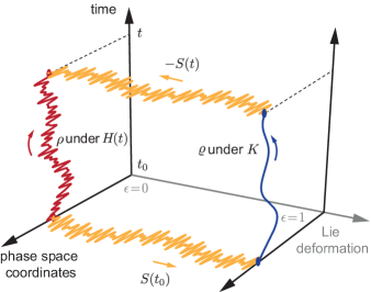
Figure 1: Time-evolution of the state vector in the transformed and un-transformed frames. The red curve represents the complicated time-evolution of $\rho$ under the time-dependent $H$. The blue curve represents the simpler time-evolution of $\varrho$ under the time-independent $K$. The transformation is exact. Under a sufficiently fast oscillating drive, the fast micromotion captured by $S$ can be neglected and $K$ can be taken to generate the time-evolution of $\rho$ in the un-transformed frame.

In the transformed representation, the dynamics obeys formally (1) as $\partial_{t}{\varrho}\!=\!\{\!\!\{K,\varrho\}\!\!\}$, with the Kamiltonian $K$ given by

$$K=e^{L_{S}}H+\int_{0}^{1}d\epsilon\,e^{\epsilon L_{S}}\dot{S};$$ (4)

see Supplementary material Section A for the derivation. Note that in the quantum case, Eq. 4 reduces to the familiar expression $\hat{K}=\hat{U}^{\dagger}(\hat{H}-i\hbar\partial_{t})\hat{U}$ with $\hat{U}=e^{-\hat{S}/i\hbar}.$

We now carry out a perturbative expansion generated by $S$, while imposing that $K$ is rendered time-independent. The transformation of the time-evolution from $\rho\rightarrow\varrho$ is represented schematically in Fig. 1 and yields

$$\begin{split}\rho&=\mathcal{T}e^{\int_{t_{0}}^{t}dt^{\prime}\,L_{H(t^{\prime})}}\rho_{0}\\ &=e^{L_{-S(t)}}e^{L_{K}(t-t_{0})}e^{L_{S(t_{0})}}\rho_{0},\end{split}$$ (5)

where $\mathcal{T}$ is the time-ordering operator and $\rho_{0}$ is the initial state. The time-evolution of $\rho$ under $H$ (a Lie transformation generated by $H$ and parametrized by $t$) can be understood as being decomposed into three successive Lie transformations generated by $S(t_{0})$, $K$, and $-S(t)$. Under this decomposition, the time-ordering operator drops out in the time-evolution under $K$, providing an important simplification.

To carry out the perturbative expansion, we consider the Hamiltonian

$$H(t)=\sum_{m\in\mathbb{Z}}H_{m}e^{im\omega t}$$ (6)

with period $T=2\pi/\omega$. For the perturbative treatment to be valid, the rate of evolution under any one $H_{m}$ needs to be much smaller than $\omega$. In the case of an unbounded Hamiltonian, either quantum or classical, the corresponding space will require truncation. We focus on the case of a periodic drive for simplicity but we note that our treatment can be generalized to include quasiperiodic or non-monochromatic drives; see Supplement section B III. We take as an ansatz for $S$ and $K$

$$S =\sum_{n\in\mathbb{N}}S^{(n)}, {K} =\sum_{n\in\mathbb{N}}{K}^{(n)},$$ (7)

where we take $S^{(0)}=0$ and the $n^{\mathrm{th}}$ terms to be of order $n$ in the expansion parameter, here taken to be $1/\omega$. Substituting Eqs. (7) into Eq. 4 separates the problem into orders of $1/\omega$. At each order, $K^{(n)}$ can further be expressed as a sum of terms generated by a Lie series as in Eq. 3, which we write as $K^{(n)}=\sum_{k}K^{(n)}_{[k]}$. Demanding $K$ to be time-independent to all orders, we find, after a few lines of algebra, the following coupled recursive formulas:

$${K}_{[k]}^{(n)}\;\;\; =\begin{cases}H&n=k=0\\ \dot{S}^{(n+1)}+L_{S^{(n)}}H&k=1\\ \sum\limits_{m=0}^{n-1}\frac{1}{k}L_{S^{(n-m)}}{K}_{[k-1]}^{(m)}&1<k\leq n+1\\ 0&\text{otherwise},\end{cases}$$ (8a)

$${S}^{(n+1)} =\begin{cases}-\int dt\,\mathrm{\textbf{osc}}(H)&n=0\\[2.0pt] -\int dt\,\mathrm{\textbf{osc}}\Big{(}L_{S^{(n)}}H&\\ \;\;+\sum\limits_{k>1}^{n+1}\sum\limits_{m=0}^{n-1}\frac{1}{k}L_{S^{(n-m)}}{K}_{[k-1]}^{(m)}\Big{)}&n>0,\end{cases}$$ (8b)

where $$\mathrm{\textbf{osc}}(f)\coloneqq f-\overline{f} \overline{f}=\frac{1}{T}\int_{0}^{T}dt\,f H$$, and . Note that is taken to be of order zero in the perturbation parameter, but this hypothesis can be relaxed in a more elaborate treatment; see Supplement section B III.

By construction, taking the time-derivative of Eq. 8b, substituting the result into Eq. 8a, and summing over $k$ yields a time-independent $K^{(n)}$. All in all, the computations of $K$ and $S$ are interleaved so that the computation of $K^{(n)}$ requires as an input the value of $S^{(m\leq n)}$. Demanding the time-independence of $K^{(n)}$ fixes $\dot{S}^{(n+1)}$, allowing the recursion to be carried out to the next order. The coupled recursive formula in Eq. 8 constructs, as announced, $S$ and $K$ order-by-order.

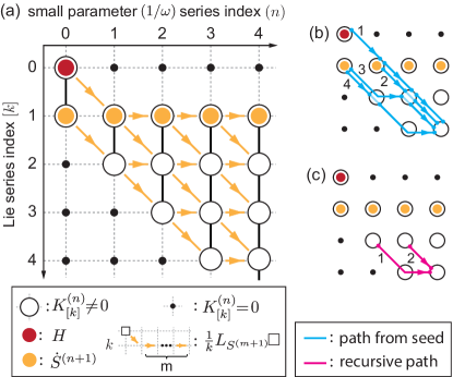
Figure 2: (a) Grid for the diagrammatic construction of $K$ and $S$. Colored circles represent the seeds generating the series to all orders. (b) As an example, all the paths contributing to the calculation of $K^{(3)}_{[3]}$ are highlighted. (c) Here, only the subpaths contributing to the recursive expression of the same term are highlighted.

The mathematical structure of the recursive formula Eq. 8 is shown diagrammatically in Fig. 2, as we now explain. The figure consists of a grid indexed by the integers $n$ and $k$. The grid supports a graph. Each node $(n,k)$ of the graph corresponds to a summand $K^{(n)}_{[k]}$, and the colored ones represent the “seeds” of the calculation. The summand $K^{(n)}_{[k]}$ is itself a sum of terms, each corresponding to a path connecting the node $(n,k)$ to a seed. Evaluating a path corresponds to taking Lie derivatives over $H$ or $\dot{S}^{(n+1)}$ as dictated by the seed color. The rule is that each Lie derivative is specified by a valid subpath, which must start “downwards” and, when followed by $m$ horizontal edges at row $k$, contributes with $L_{S^{(m+1)}}/k$. Finally, if the considered node is itself colored, either $H$ or $\dot{S}^{(n+1)}$ must be added to the sum. We note that our grid construction is inspired by Deprit (1969), where the construction is limited to completely classical and time-independent systems.

Let us discuss, as an example, how $K^{(3)}_{[3]}$ is evaluated from the figure. As indicated by panel Fig. 2(b), $K^{(3)}_{[3]}$ contains only four terms corresponding to the concatenations of the valid subpaths (in blue). The sum reads

$$\begin{split}K^{(3)}_{[3]}={}&\frac{L_{S^{(1)}}}{1}\frac{L_{S^{(1)}}}{2}\frac{L_{S^{(1)}}}{3}H+\frac{L_{S^{(1)}}}{2}\frac{L_{S^{(1)}}}{3}\dot{S}^{(2)}\\ &{}+\frac{L_{S^{(1)}}}{2}\frac{L_{S^{(2)}}}{3}\dot{S}^{(1)}+\frac{L_{S^{(2)}}}{2}\frac{L_{S^{(1)}}}{3}\dot{S}^{(1)},\end{split}$$

where the terms are ordered as enumerated in the figure.

Alternatively, one could have expressed $K^{(3)}_{[3]}$ recursively by directly applying Eq. 8a. The computation of $K^{(3)}_{[3]}$ then involves only the two pink subpaths shown in Fig. 2(c) and yields

$$K^{(3)}_{[3]}=\frac{L_{S^{(2)}}}{3}K^{(1)}_{[2]}+\frac{L_{S^{(1)}}}{3}K^{(2)}_{[2]}.$$

At this stage, once all entries of the $n^{\mathrm{th}}$ column are computed, the calculation proceeds by demanding the time-independence of $K^{(n)}$ computed as their row-sum over column $n$ and represented by the vertical bold lines in Fig. 2(a). This is required by Eq. 8b. For the column $n=3$ the algorithm yields

$$S^{(4)}=-\int dt\,\mathrm{\textbf{osc}}\left(L_{S^{(3)}}H+K^{(3)}_{[2]}+K^{(3)}_{[3]}+K^{(3)}_{[4]}\right),$$

which is a necessary ingredient to compute $K^{(5)}$ and so, the calculation proceeds.

The formulation is further illustrated by treating as concrete examples the classical and quantum Kapitza pendulum and the driven Duffing oscillator in Section B of the Supplementary material. Moreover, we also present in section B III the remarkable agreement with recent experiments Eickbusch et al. (2021) that independently measures the effective Hamiltonian of a driven transmon-cavity superconducting circuit and has been only analyzed numerically until now.

We stress again that Eq. 8 is agnostic to the choice of Lie bracket in Eq. 2. A Lie-based formulation is thus well-suited to unify seemingly disconnected perturbation methods, in particular those that, to be linked, require the quantum-classical correspondence to be made explicit.

Exploiting this property, we now turn to discuss the connection between several time-dependent perturbation methods developed independently. We consider their common starting point to be the additive ansatz

$$Z=\mathcal{Z}+\zeta(\mathcal{Z},^{c}\!\!\mathcal{Z}),$$ (9)

where $Z$ is the state variable, ${}^{c}\!\mathcal{Z}$ is the conjugate variable to $\mathcal{Z}$ and $\zeta$ is a correction. For time-varying problems, it is customary to take $\mathcal{Z}$ to describe the slow dynamics and the correction to describe the fast dynamics with vanishing time-average ($\bar{\zeta}\!=\!0$). To compute $\zeta$, different methods proceed in vastly different ways: the classical ones rely on partial derivatives of phase-space functions Krylov and Bogoliubov (1937); Bogoliubov and Mitropolsky (1961); Landau and Lifshitz (1976); Rahav et al. (2003); this draws a line separating them from the quantum methods which rely on matrix products Rahav et al. (2003); Eckardt and Anisimovas (2015); Casas et al. (2001); Mirrahimi and Rouchon (2015); Mikami et al. (2016); Xiao et al. (2021). These procedural differences hide their shared structure.

We uncover the connection between these methods by realizing that the procedural differences stem from premature specifications of a particular Lie bracket. Identifying this feature allows us to relate the correction $\zeta$, specified by each method, to the generator $S$ of the Lie transformation as $\zeta\!\!=\!\!(e^{L_{-S}}\!\!-\!\!I)\mathcal{Z}$. In other words, the ansatz in Eq. 9 corresponds to the additive representation of the exponential map in Eq. 3. It follows that, if carried out to all orders, these methods correspond to invertible canonical transformations. See Section C of the Supplementary material for a detailed discussion on the relationship between the different ansätzs.

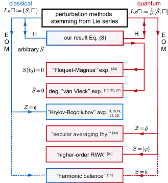
Figure 3: Relationship between various perturbation methods for systems submitted to a time-dependent oscillatory drive. All the methods in the tree can be seen as falling under the umbrella of Lie series. The methods can be divided between classical (blue lines-left) and quantum (red lines-right) ones. Other forks separate the methods based on the equation of motion (EOM) from the methods based on the Hamiltonian (H). The dashed lines refer to a class of methods whose effective Hamiltonians have not yet been identified and they are left for future work. The methods labeled by a $\mathcal{Z}$ symbol are additive ansatz-based unlike the methods containing $S$ which can be thought as multiplicative. For the Hamiltonian methods, the associated integration constant for $S$ in Eq. 8b is specified as a condition. The acronym RWA stands for rotating wave approximation. The double arrow refers to a bidirectional relationship.

In Fig. 3, we show how we can collect seemingly disconnected perturbation methods and unify them under the umbrella of Lie series. The two main branches, colored in red (right) and blue (left), group the quantum and classical methods. The ones based on equations of motion (EOM) correspond to different choices of $Z$ in Eq. 9. Among the quantum methods, secular averaging theory (SAT) Buishvili and Menabde (1979) corresponds to $Z\!\!=\!\!\hat{\rho}$. The perturbative expansion can also be developed at the level of the wave function $Z\!\!=\!|\phi\rangle$, allowing for the derivation of higher-order rotating wave approximations (RWA) Mirrahimi and Rouchon (2015). In this case, the ansatz is $\mathcal{Z}\!\!=\!|\varphi\rangle$ and $\zeta\!\!=\!\hat{\delta}|\varphi\rangle$ and it can be mapped to our approach by taking $\zeta\!\!=\!\!(e^{-\hat{S}/i\hbar}\!-1)|\varphi\rangle$. This last relation can be understood by noting that in the quantum case Eq. 3 reduces to $e^{L_{S}}\hat{\rho}\!=\!e^{-\hat{S}/i\hbar}\hat{\rho}e^{\hat{S}/i\hbar}$. Classically, the Krylov-Bogoliubov (KB) method Krylov and Bogoliubov (1937); Bogoliubov and Mitropolsky (1961); Rahav et al. (2003); Landau and Lifshitz (1976); Nayfeh (2008) averages the equation of motion of the position coordinate $\mathcal{Z}\!\!=\!\mathfrak{q}$ and $\zeta\!\!=\!\zeta(\mathfrak{q},\mathfrak{p},t)$, where $\mathfrak{p}$ is the conjugate momentum, and it maps to our approach with $\zeta\!\!=\!\!(e^{L_{S}}-I)\mathfrak{q}$ (the change of sign in $S$ is simply a change from the active representation used so far to the passive representation used in KB).

Besides the EOM methods, we also include the most common quantum Hamiltonian methods in the genealogy of Fig. 3. They are characterized by the utilization of Floquet theorem Shirley (1965), which guarantees the existence of a unitary transformation rendering the Kamiltonian time-independent. They map naturally to the exponential representation discussed in this work. We find that using the freedom in the integration constant of Eq. 8b, as specified in Fig. 3, we recover the so-called Floquet-Magnus expansion $(S(t_{0})=0)$ Casas et al. (2001) or the van Vleck expansion ($\bar{S}=0$) Rahav et al. (2003); Eckardt and Anisimovas (2015); Xiao et al. (2021). This gives formal ground to the observations made in Bukov (2017); Mikami et al. (2016) on the connection between these two methods.

Note that, with the exception of the Floquet-Magnus expansion, all the aforementioned methods were limited to the lowest orders. Instead, our symbolic formula can be readily used to carry out the calculation to arbitrary order. We illustrate this by taking as an example the widely employed van Vleck expansion. We have explicitly written a symbolic algebra algorithm, made available in vv2 (2021), and used it to explicitly display the expansion up to order five, automatedly (see Section D of the Supplementary material). To the best of our knowledge, the expansion could only be found to order three in the literature Mikami et al. (2016) until now.

In this article, we developed a perturbation method to treat rapidly driven nonlinear systems yielding a double coupled recursive formula well-suited for symbolic computation. The construction can thus be carried out in an automated way to arbitrary order. We achieve this by constructing a canonical transformation that explicitly decouples the relevant dynamics, governed by a time-independent effective Hamiltonian, from the complicated micromotion. Our treatment is completely agnostic to the classical or quantum nature of the problem and sheds light on the longstanding discussion of the relationship between well-known perturbation methods developed independently of each other. We remark that our formula can be generalized to treat Hamiltonians of arbitrary order in the perturbation parameter. This is particularly powerful when treating parametric processes in driven nonlinear bosonic oscillators Xiao et al. (2022), paving the way for Hamiltonian engineering in superconducting quantum circuits. Finally, we note that there is a strong relationship between time-periodic (Floquet) and space-periodic (Bloch) systems, and thus, our recursive formula can be adapted to compute the Schrieffer-Wolff transformation Bravyi et al. (2011) to arbitrary order and potentially get new results in quantum many-body problems.

We acknowledge Shoumik Chowdhury, Mark Dykman, Steve Girvin, Leonid Glazman, Pratyush Sarkar, and Yaxing Zhang for insightful discussions. We also thank Hideo Aoki and Sota Kitamura for a discussion on their classification of terms in the van Vleck expansion. This research was supported by the National Science Foundation (NSF) under grant number 1941583, the Air Force Office of Scientific Research (AFOSR) under grant number FA9550-19-1-0399, and the Army Research Office (ARO) under grant number W911NF-18-1-0212. The views and conclusions contained in this document are those of the authors and should not be interpreted as representing the official policies, either expressed or implied, of the NSF, the AFOSR, the ARO, or the U.S. Government. The U.S. Government is authorized to reproduce and distribute reprints for Government purposes notwithstanding any copyright notation herein.

References

- Dykman (2012) M. Dykman, Fluctuating nonlinear oscillators: from nanomechanics to quantum superconducting circuits (Oxford University Press, 2012).
- Guckenheimer and Holmes (2013) J. Guckenheimer and P. Holmes, Nonlinear oscillations, dynamical systems, and bifurcations of vector fields, vol. 42 (Springer Science & Business Media, 2013).
- Zurek and Paz (1999) W. H. Zurek and J. P. Paz, in Epistemological and Experimental Perspectives on Quantum Physics (Springer, 1999), pp. 167–177.
- Landau and Lifshitz (1976) L. D. Landau and E. M. Lifshitz, Mechanics: Volume 1, vol. 1 (Butterworth-Heinemann, 1976).
- Bechhoefer (2021) J. Bechhoefer, Control Theory for Physicists (Cambridge University Press, 2021).
- Leghtas et al. (2015) Z. Leghtas, S. Touzard, I. M. Pop, A. Kou, B. Vlastakis, A. Petrenko, K. M. Sliwa, A. Narla, S. Shankar, M. J. Hatridge, et al., Science 347, 853 (2015).
- Lescanne et al. (2020) R. Lescanne, M. Villiers, T. Peronnin, A. Sarlette, M. Delbecq, B. Huard, T. Kontos, M. Mirrahimi, and Z. Leghtas, Nature Physics 16, 509 (2020).
- Grimm et al. (2020) A. Grimm, N. E. Frattini, S. Puri, S. O. Mundhada, S. Touzard, M. Mirrahimi, S. M. Girvin, S. Shankar, and M. H. Devoret, Nature 584, 205 (2020).
- Haroche and Raimond (2006) S. Haroche and J.-M. Raimond, Exploring the quantum: atoms, cavities, and photons (Oxford university press, 2006).
- Chamberland et al. (2020) C. Chamberland, K. Noh, P. Arrangoiz-Arriola, E. T. Campbell, C. T. Hann, J. Iverson, H. Putterman, T. C. Bohdanowicz, S. T. Flammia, A. Keller, et al., arXiv preprint arXiv:2012.04108 (2020).
- Goldman and Dalibard (2014) N. Goldman and J. Dalibard, Phys. Rev. X 4, 031027 (2014).
- Wintersperger et al. (2020) K. Wintersperger, C. Braun, F. N. Ünal, A. Eckardt, M. Di Liberto, N. Goldman, I. Bloch, and M. Aidelsburger, Nature Physics 16, 1058 (2020).
- Yao et al. (2017) N. Y. Yao, A. C. Potter, I.-D. Potirniche, and A. Vishwanath, Phys. Rev. Lett. 118, 030401 (2017).
- Nandkishore and Huse (2015) R. Nandkishore and D. A. Huse, Annu. Rev. Condens. Matter Phys. 6, 15 (2015).
- Nayfeh (2008) A. H. Nayfeh, Perturbation methods (John Wiley & Sons, 2008).
- Eckardt (2017) A. Eckardt, Reviews of Modern Physics 89, 011004 (2017).
- Blais et al. (2021) A. Blais, A. L. Grimsmo, S. M. Girvin, and A. Wallraff, Rev. Mod. Phys. 93, 025005 (2021).
- Zeuch et al. (2020) D. Zeuch, F. Hassler, J. J. Slim, and D. P. DiVincenzo, Annals of Physics 423, 168327 (2020), ISSN 0003-4916.
- Rahav et al. (2003) S. Rahav, I. Gilary, and S. Fishman, Phys. Rev. A 68, 013820 (2003).
- Bukov (2017) M. Bukov, Ph.D. thesis, Boston University (2017).
- Krylov and Bogoliubov (1937) N. M. Krylov and N. N. Bogoliubov, Introduction to non-linear mechanics (In Russian) (Ac. of Sci. Ukr. SSR, 1937), [English translation by Princeton University Press, Princeton, 1947].
- Bogoliubov and Mitropolsky (1961) N. N. Bogoliubov and Y. A. Mitropolsky, Asymptotic methods in the theory of non-linear oscillations (In Russian) (1961), [English translation by Hindustan Pub., Delhi, 1961; Gordon and Breach, New York, 1961].
- Casas et al. (2001) F. Casas, J. A. Oteo, and J. Ros, Journal of Physics A, Mathematical and General 34, 3379 (2001), ISSN 0305-4470.
- Mirrahimi and Rouchon (2015) M. Mirrahimi and P. Rouchon, Dynamics and control of open quantum systems (2015).
- Eckardt and Anisimovas (2015) A. Eckardt and E. Anisimovas, New journal of physics 17, 093039 (2015).
- Mikami et al. (2016) T. Mikami, S. Kitamura, K. Yasuda, N. Tsuji, T. Oka, and H. Aoki, Physical Review B 93, 144307 (2016).
- Xiao et al. (2021) Z. Xiao, E. Doucet, T. Noh, L. Ranzani, R. Simmonds, L. Govia, and A. Kamal, arXiv preprint arXiv:2103.09260 (2021).
- Petrescu et al. (2020) A. Petrescu, M. Malekakhlagh, and H. E. Türeci, Phys. Rev. B 101, 134510 (2020).
- Groenewold (1946) H. J. Groenewold, in On the Principles of Elementary Quantum Mechanics (Springer, 1946), pp. 1–56.
- Moyal (1949) J. E. Moyal, Mathematical Proceedings of the Cambridge Philosophical Society 45, 99–124 (1949).
- Zachos et al. (2005) C. Zachos, D. Fairlie, and T. Curtright (2005).
- Dragt and Finn (1976) A. J. Dragt and J. M. Finn, Journal of Mathematical Physics 17, 2215 (1976).
- Deprit (1969) A. Deprit, Celestial mechanics 1, 12 (1969).
- Eickbusch et al. (2021) A. Eickbusch, V. Sivak, A. Z. Ding, S. S. Elder, S. R. Jha, J. Venkatraman, B. Royer, S. Girvin, R. J. Schoelkopf, and M. H. Devoret, arXiv preprint arXiv:2111.06414 (2021).
- Buishvili and Menabde (1979) L. L. Buishvili and M. G. Menabde, Theoretical and Mathematical Physics 50, 2435 (1979).
- Shirley (1965) J. H. Shirley, Physical Review 138, B979 (1965).
- vv2 (2021) https://github.com/xiaoxuisaac/vanVleck-recursion (2021).
- Xiao et al. (2022) X. Xiao, J. Venkatraman, R. G. Cortiñas, A. Eickbusch, S. Chowdhury, and M. H. Devoret, In Preparation (2022).
- Bravyi et al. (2011) S. Bravyi, D. P. DiVincenzo, and D. Loss, Annals of Physics 326, 2793 (2011), ISSN 0003-4916.