Attention-based fusion of semantic boundary and non-boundary information
to improve semantic segmentation

Abstract

This paper introduces a method for image semantic segmentation grounded on a novel fusion scheme, which takes place inside a deep convolutional neural network. The main goal of our proposal is to explore object boundary information to improve the overall segmentation performance. Unlike previous works that combine boundary and segmentation features, or those that use boundary information to regularize semantic segmentation, we instead propose a novel approach that embodies boundary information onto segmentation. For that, our semantic segmentation method uses two streams, which are combined through an attention gate, forming an end-to-end Y-model. To the best of our knowledge, ours is the first work to show that boundary detection can improve semantic segmentation when fused through a semantic fusion gate (attention model). We performed an extensive evaluation of our method over public data sets. We found competitive results on all data sets after comparing our proposed model with other twelve state-of-the-art segmenters, considering the same training conditions. Our proposed model achieved the best mIoU on the CityScapes, CamVid, and Pascal Context data sets, and the second best on Mapillary Vistas.

1 Introduction

Many vision-related applications rely on semantic segmentation to evaluate visual contents and perform decision making. For example, autonomous driving (Cordts et al., 2016; Neuhold et al., 2017), agricultural automation (Santos et al., 2020), medical image analysis (Bakas et al., 2017), remote sensing imagery (Maggiori et al., 2017), and the human parsing task (Liang et al., 2015) usually leverage the semantics of pixel-level labels to obtain valuable information such as an object class, location, or shape.

As with many vision-based tasks, the current state-of-the-art in semantic segmentation heavily explores convolutional neural networks (CNN), being DeepLabV3 (Chen et al., 2017), DeepLabV3+ (Chen et al., 2018), and PSPNet (Zhao et al., 2017) some of the best architectures in the current literature. In particular, fully convolutional networks (FCN) (Long et al., 2015), which are usually used as the main branch of the CNN-based segmenters, have achieved high-quality results as demonstrated by several works (Chen et al., 2018; Zhao et al., 2017; Rota Bulò et al., 2018; Ronneberger et al., 2015; Badrinarayanan et al., 2017). FCN-based models use pre-trained classification networks to obtain a score-map that relates classes to each pixel of the input image. During this process, the classification networks downsample the map of features, progressively reducing the spatial resolution of the original input. The information loss that ensues from this downsampling is particularly relevant to semantic segmentation. The decrease of resolution causes the loss of detail, resulting in lower accuracy for smaller objects and boundary regions in general.

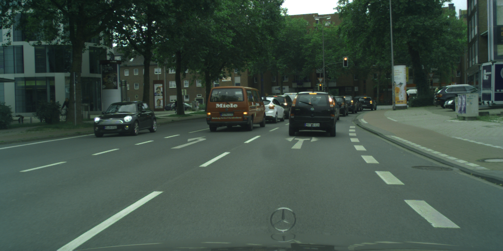
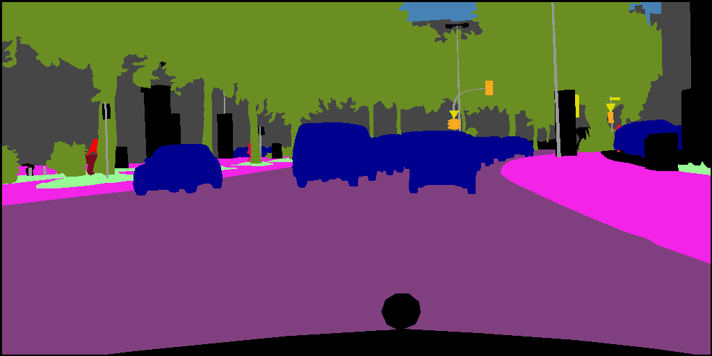
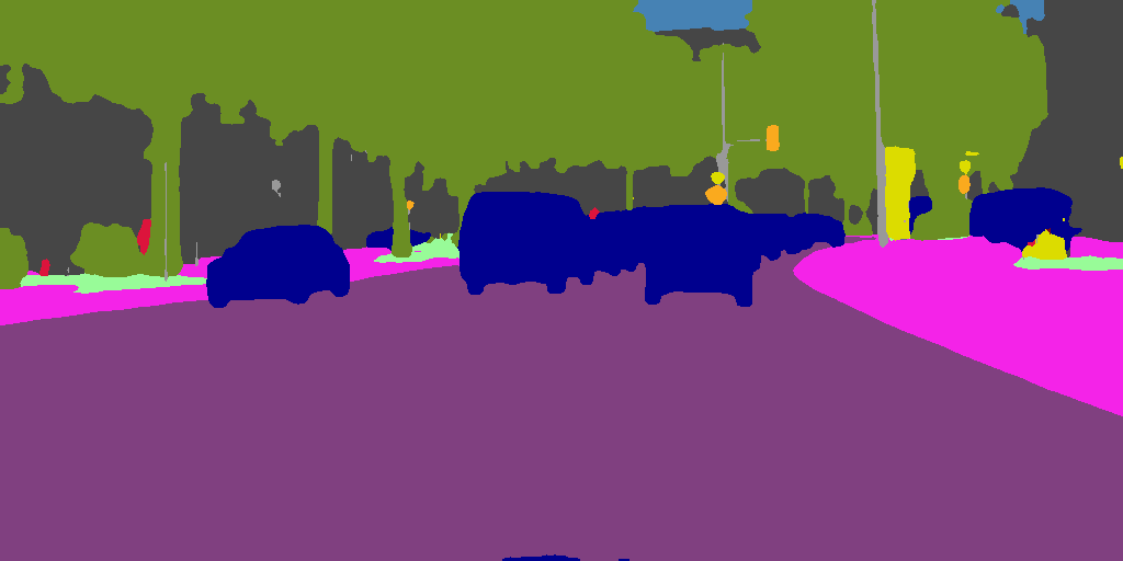
Figure 1: How important are the boundaries in the process of image segmentation. (a) An image sample from Cityscapes (Cordts et al., 2016), (b) the ground truth, (c) the masks predicted by DeepLabV3(Chen et al., 2017), and (d) difference between (b) and (c).

Commonly segmentation models face problems in segmenting the boundaries and their surroundings. Figure 1 shows the result of the semantic segmentation obtained by a DeepLabV3 (Chen et al., 2017) network compared to the ground truth. The difference between ground truth (Figure 1(b)) and prediction (Figure 1(c)), depicted in Figure 1(d), indicates that a large part of the error attributed to the model is related to boundary regions, further reinforcing the hypothesis that semantic boundaries should be included as part of the problem modeling. To minimize that problem, one could use a semantic boundary detection (SBD) module (Yu et al., 2017b; Acuna et al., 2019; Hu et al., 2019; Ma et al., 2020). By adding an SBD module to an FCN segmentation architecture, a new relevant challenge is introduced: How to determine adequate pixel context from boundary and segmentation information separately? A promising avenue of investigation to address this question is to use attention gates, which are usually explored to combine low-level features and high-level features in deep architectures (Fu et al., 2020). In our work, we propose a novel approach that uses attention gate to help separate boundary and non-boundary information, seeking for the improvement of the semantic segmentation results. We investigate whether the use of semantic segmentation and SBD, combined through an attention model, can contribute to better results in semantic segmentation. The rationale is that it is possible to separately learn from different contexts by using attention models, also jointly training the model in an end-to-end network. We argue that the pixels belonging to the object boundaries have different characteristics when compared to the other image pixels, and this difference is mainly related to the context of border pixels containing features from both objects separated by that border.

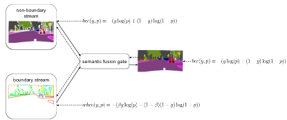
Figure 2: Our proposed Y-model is comprised of three parts: Non-boundary stream, boundary stream, and a semantic fusion gate. The semantic fusion gate is an attention gate in charge of combining the network signal of the boundary and non-boundary streams in the forward step (segmentation), while splitting the error signal in the backward step (training).

Figure 2 illustrates our approach to the problem of semantic segmentation. We call it Y-model mainly because of the shape of the network. The semantic fusion gate is an attention gate in charge of combining the network signals ( ) of the boundary and non-boundary streams in the forward step (segmentation) while splitting the error signals ( ) in the backward step (training). Each stream and and the top of the attention gate have its own loss function. All losses are used to optimize the entire network all at once in an end-to-end way. We performed experiments to validate our proposal using four publicly available data sets, that are: Cityscapes (Cordts et al., 2016), Mapillary Vistas (Neuhold et al., 2017), CamVid (Brostow et al., 2008), and Pascal Context (Mottaghi et al., 2014). Cityscapes, Mapillary Vistas, and CamVid are composed of traffic images from the driver’s viewpoint, while Pascal Context is a data set that presents a diversity of scenes, without theme restriction on the class sets.

The data sets used for experimentation are all burdened by the class imbalance problem. For instance, in Cityscapes, Mapillary Vistas, and CamVid, the volume of pixels belonging to the class “road” is much higher in scale than the other classes in any given scene (due to the inherent nature of traffic-related footage). To reduce the impact that unbalanced data may have, works such as in (Takikawa et al., 2019) and (Zhu et al., 2019) proposed methods that attempt to enforce uniform class distribution by selecting particular crops from the original image during training. In (Takikawa et al., 2019), classes, which have a less overall frequency in the data set, are selected, assuring that whenever these classes are present in the image, they are also present in the selected crop. In (Zhu et al., 2019), centroids are computed from the image segments and then the crop is selected by considering a uniform sampling of these centroids. In our work, we propose a new method for crop selection in unbalanced data sets. Unlike (Takikawa et al., 2019) and (Zhu et al., 2019), our method assigns a weight value to each pixel from each image on the data set. These weight values are inversely proportional to the class frequencies in the overall data set. This approach makes it possible to perform crops that minimize the class unbalance issue on the training data by considering the value of each pixel of the image during crop selection.

1.1 Contributions

The main contributions of this work are summarized as follows: A new model comprised of non-boundary and boundary streams that divides the tasks of semantic segmentation and semantic boundary detection by means of a Y-model and an attention gate, and a new strategy for uniform crop selection that efficiently reduces the imbalance of the classes in the training data sets

2 Related work

Here we briefly go over the relevant published works on topics that directly or indirectly impacted our proposed model. They are semantic segmentation, boundary detection, semantic boundary detection, and attention models.

Semantic segmentation

FCN-based models usually own three modules: A feature extractor that uses an image classification network (backbone), without the dense layers at the end; a module that tries to expand the receptive field through dilated convolutions (Yu and Koltun, 2015; Chen et al., 2017; Yang et al., 2018), large convolutions (Peng et al., 2017), and image pooling (Zhao et al., 2017; Liu et al., 2015); and a decoder in charge of combining the extracted features while performing pixel-wise classification to produce the segmentation map. One significant issue of FCN-based approaches is related to the spatial representation of the extracted features. The downsampling stages of the classification network reduce the spatial resolution of the features, effectively attenuating the object boundaries in the input image. Due to this effect, FCN-based segmentation networks usually produce results with less detailed boundaries when compared to the ground truth.

Some works manage to improve accuracy on the boundaries by using features from different stages of the backbone (Long et al., 2015; Zhou et al., 2018; Chen et al., 2018). The rationale is that features from the early stages have better spatial representation since they are not as downsampled as features from later stages. Models such as FCN-8 (Long et al., 2015) and DeeplabV3+ (Chen et al., 2018) are examples of the networks that improve their overall results by exploiting features of the initial stages of a ResNet network (He et al., 2016). However, even when combining several stages of the backbone, a significant part of the classification errors in segmentation models still occur due to failures in boundary classification, as illustrated by Figure 1, where the difference between the segmentation result and the ground truth is mostly defined by incorrectly-classified boundaries. These results indicate that networks trained solely for semantic segmentation have difficulty in segmenting the borders of the objects. Simply using various stages of the backbone is not enough to completely overcome the problem of poor classification rate on the boundaries.

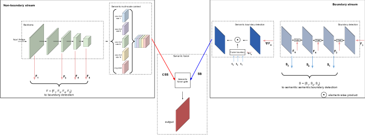
Figure 3: Detailed architecture of our Y-model. The input image is fed to a backbone that generates a set of features maps (F) with different scales. The feature maps F are used in the boundary stream to obtain a set of features S. Each element in S represents the boundary from the features of different scales in F. The semantic boundary detection module combines $F_{5}$ and S to obtain the semantic boundaries (SE), which combined with the coarse semantic segmentation (CSS) through the attention gate output the segmented image.

Boundary detection

Some methods explore deep networks to detecting boundary (Xie and Tu, 2015; Le and Duan, 2020) and semantic boundary (Yu et al., 2018b). The results obtained by these methods surpass those based on hand-crafted features. For instance, Takikawa et. al. (Takikawa et al., 2019) use boundary detection to improve semantic segmentation by creating a branch that combines features extracted from several stages of a ResNet (He et al., 2016) network. The feature learning is then split through a gate-based model into two different streams, one for the boundaries and the other for semantic segmentation.

Semantic boundary detection

More recently, methods that detect boundaries for each semantic class (Yu et al., 2017b; Acuna et al., 2019; Hu et al., 2019; Ma et al., 2020) have obtained better results than those that perform general boundary detection. This motivated us to use semantic borders as part of our method. One should note that those works do not perform semantic segmentation, but only boundary detection.

Attention models

To build a multi-task neural network, there is usually the need to compound multiple loss functions and a clear strategy as to how to combine the multiple tasks. In (Yu et al., 2017b), the use of a specific loss function based on binary cross-entropy is proposed as a way to deal with boundary classification. In our experiments, however, we have noticed that when combining regular semantic segmentation features with boundary features, the training gradient ends up attenuating the signal coming from the boundary detection stream.

3 Fusion of boundary and non-boundary information through an attention gate

We explored an attention-gate approach, explicitly modeling object boundaries as a way to improve semantic segmentation. To do so, we conceived a Y-model (refer to Figure 2) defined by three components: A non-boundary stream, which produces a coarse segmentation for the input image; a boundary stream, responsible for processing the input features to perform border detection; and a semantic fusion gate (attention model), which integrates both streams to obtain the final semantic segmentation output. Figure 3 shows in detail our complete proposed architecture. The streams are each one split into two different processing steps. The non-boundary stream is represented by the backbone and semantic multi-scale context modules, while the boundary stream is represented by the boundary detection and semantic boundary detection modules. Both streams are processed in parallel, and their outputs are combined to produce the final output via a semantic fusion gate.

3.1 Non-boundary stream

The non-boundary stream is responsible for performing a preliminary semantic segmentation step on the input image. As previously mentioned, we based our Y-model in an FCN-based network. These types of networks consist of three modules: The first is a feature extractor, which uses an image classification network as backbone. The one-by-one convolution, usually placed at the end of the network for class prediction, is excluded; the second module improves the context representation of each pixel by using dilated convolutions (Yu and Koltun, 2015; Chen et al., 2017; Yang et al., 2018), large convolutions (Peng et al., 2017), and image pooling (Zhao et al., 2017; Liu et al., 2015); the last and third module is the decoder. The decoder is responsible for combining the extracted features and performing pixel classification to produce the segmentation map. The backbone used by our proposed model relies in five stages as illustrated on the top-left part of Figure 3. We applied an FCN-based network that takes as input an image $I\in\mathbb{R}^{H\times W\times C}$ with height $H$ and width $W$, and the number of channels $C$ that outputs a map $M$ of dimensions $H\times W$. A coarse semantic segmentation ($\mathbf{CSS}$) map contains the class prediction scores for each pixel in the image, which is ultimately refined by the output of the boundary stream.

Backbone

As the base feature extractor for the non-boundary and boundary streams, we used a Dilated ResNet (Yu et al., 2017a) (with 50 and 101 layers) and a WideResNet (Zagoruyko and Komodakis, 2016) (38 layers), in our experiments. For the Dilated ResNet, we used the default dilation rates of 2 and 4 in blocks 4 and 5 of our network, respectively, producing an output with stride 8. This design choice follows the suggestions in (Yu et al., 2017a). For the WideResNet, we used a dilation rate of 2 for block 3, and a dilation rate of 4 for the subsequent blocks. This final output is achieved with stride 4. The feature extractors structured with dilated convolution increment the feature output shapes, improving the image representation for the segmentation task.

Semantic multi-scale context

We used a multi-scale representation for the context. This is done by way of an atrous spatial pyramid pooling (ASPP) (Chen et al., 2017) module, which captures multi-scale contextual information using dilated convolutions with different dilation rates. For both training and testing, we used an output stride of 8.

3.2 Boundary stream

The boundary stream works essentially as a boundary-detector in our proposed model. It takes as input the same image $I$ as the non-boundary stream, and output a segmentation map highlighting object boundaries as depicted in Figure 2.

Boundary detection

We extract features from different stages of the backbone to improve the prediction accuracy on the boundaries. Features from five different stages, denoted as $F_{1}$, $F_{2}$, $F_{4}$, $F_{5}$, feed the semantic boundary detection module, as depicted in Figure 3. The boundary detection module progressively combines the features $F_{1}$, $F_{3}$, $F_{4},$ $F_{5}$ through gates (see the boundary detection module in Figure 3) in order to output a set of features $S_{n}\in\{S_{1},S_{2},S_{3}\}$ representing the different processing stages on the boundary that go to the semantic boundary detection module. The use of these gates are necessary to facilitate the flow of information from the non-boundary stream to the boundary stream. Each gate selects from the input features the information that is relevant to perform boundary detection, thus effectively separating the relevant activations to the segmentation from those relevant to the boundary detection tasks. This local gate consists of an attention map $\alpha_{g}$ followed by a residual basic module. The attention map, $\alpha_{g}$, is given by

$$\alpha_{g} =\sigma(\circledast_{1\times 1}(F_{n}||{F^{\prime}}_{n}))\,,$$ (1)

where $F_{n}$ represents the backbone features from the $n_{th}$ stage used by the boundary detection module, ${\mathbf{F^{\prime}}}_{n}$ represents the pre-processed features in the boundary detection module, $||$ is the concatenation function, $\circledast_{1\times 1}$ is a convolutional layer, and $\sigma$ is the sigmoid function.

The gate, $G_{A}$, is applied to $F_{n}$, and denoted as

$$\mathrm{G_{A}} =\circledast_{1\times 1}(F_{n}\odot({\alpha_{g}}+k))\,,$$ (2)

where $\odot$ is an element-wise product. The resulting $\mathrm{G_{A}}$ is passed to a residual module, followed by a ${1\times 1}$ convolution. The final output of each gate is an $S_{n}$ map. k is a constant to reinforce the borders avoiding close-to-zero values on boundary elements.

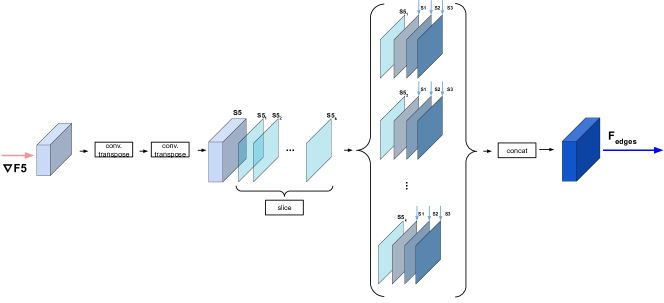
Figure 4: Fusion boundary module. The module takes as input $\nabla F_{5}$ and $S_{n}$. $\nabla F_{5}$ is resized by 2 convolution transpose layers. The result is then sliced into $S5_{k}$ feature maps, with each map being grouped by an $S_{n}$ set. Finally, an $S5_{k}$ and $S_{n}$ are concatenated and passed through a $\circledast_{1\times 1}$ layer. This module output is a feature map $\mathrm{F_{edges}}\in\mathbb{R}^{H\times W\times 4\times L}$, where $\mathrm{L}$ represents the number of classes.

Semantic boundary detection

This is inspired by the work found in (Hu et al., 2019), where the processing of low-level feature fusion is improved by more semantic features. Unlike (Hu et al., 2019), however, we used the $\nabla F_{5}$ as an input, in addition to the set of low level features $S_{n}$ in the fusion boundary module. In our fusion model, differently from what is done by the CASENet (Yu et al., 2017b) network, first we weigh the feature maps from different levels of the network to then perform the ${1\times 1}$ convolution that ultimately combines the features from multiple stages. $\nabla F_{5}$ is defined as an approximation of the gradient, and is given by

$$\nabla F_{5} \approx\sigma(F_{5}-MaxPool_{3\times 3}(F_{5})),$$ (3)

where $MaxPool_{3\times 3}$ represents a maximum-pooling operation in the 2D space with stride of 3 in both dimensions. The use of $\nabla F_{5}$ allows to obtain the most prominent features from $F_{5}$, which improves the flow of information during back-propagation.

The SBD module is divided into two components: the fusion boundary module and the attention step. The fusion boundary module is shown in Figure 4, and takes as inputs $\nabla F_{5}$ and $S_{n}$. First, $\nabla F_{5}$ is upsampled by two convolution transpose layers with stride of 8 pixels. The result is then split into $k$ slices. Each slice, $S5_{k}$, is concatenated with the $S_{n}$ sets and linearly combined by a $\circledast_{1\times 1}$. The fusion boundary module outputs the $F_{edges}$, combining the sequential application of two $\circledast_{1\times 1}$ with batch normalization and a ReLU activation function, $L_{adapt}$, through a semantic boundary attention gate, $\mathrm{SBatt}$, given by

$$\mathrm{SBatt} =L_{adapt}(\nabla F_{5})\odot F_{edges},$$ (4)

The rationale here is to reinforce the boundaries formed by both low-level and high-level features with more semantic information. Finally, the resulting $\mathrm{SBatt}$ is convoluted by a $\circledast_{1\times 1}$, resulting in the semantic boundary, $\mathbf{SB}\in\mathbb{R}^{H\times W\times L}$.

3.3 Semantic fusion gate

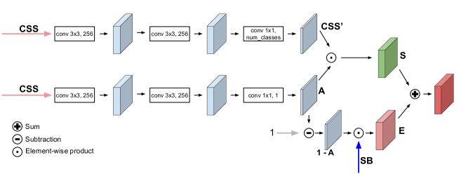
Figure 5: Details of the semantic fusion gate. The module takes as input $\mathrm{CSS}$ features, which are used in two branches. A attention gate model is applied by generating two spatial maps of attention $\mathrm{A}$ and $\mathrm{1-A}$. These maps are used to highlight the features in $\mathrm{CSS^{\prime}}$ and $\mathrm{SE}$.

Figure 5 illustrates the architecture of the semantic fusion gate, proposed in this work to separate the non-boundary and boundary information. Given a $\mathrm{CSS}\in\mathbb{R}^{H\times W\times L}$ and a semantic boundary $\mathrm{SB}\in\mathbb{R}^{H\times W\times L}$, we first feed $\mathrm{CSS}$ into 2 convolutional sets. The output of the first set is denoted as $\mathrm{CSS^{\prime}}\in\mathbb{R}^{H\times W\times L}$ features, while the second set outputs a mask, $\mathrm{A}\in\mathbb{R}^{H\times W\times L}$, that works as an attention gate. A $\mathrm{softmax}$ function is multiplied by $\mathrm{CSS^{\prime}}$, obtaining the segmentation, $\mathrm{S}$. The input $\mathrm{SB}$ is multiplied by $1-\mathrm{A}$ to get the output $\mathrm{E}$. The final segmentation is finally obtained by $\mathrm{S}+\mathrm{E}$.

The semantic fusion gate shown in Figure 5 split the semantic segmentation features into two distinct tasks. One that represents the pixels with a semantic border and the other with the pixels outside that border. This is so to avoid ambiguity in the classification of border pixels.

3.4 Multi-task loss

To train our Y-model, we used different loss functions for each sub-task. We used a weighted binary cross-entropy loss (WBCE) for the boundary stream, and a binary cross-entropy (BCE) loss for the semantic segmentation (non-boundary) stream. Our multi-task loss is modeled as

$$\mathcal{L} =\lambda_{1}\mathcal{L}_{WBCE}(s,\hat{s})+\lambda_{2}\mathcal{L}_{BCE}(y,\hat{y})\,,$$ (5)

where $\hat{s}\in\mathbb{R}^{H\times W}$ denotes the ground truth of the semantic boundaries, while $\hat{y}\in\mathbb{R}^{H\times W}$ denotes the ground truth of the semantic segmentation. $s$ and $y$ represent the predicted values of the boundary and segmentation, respectively. $\lambda_{1}$ and $\lambda_{2}$ are two hyper-parameters that control the weighting between the losses.

To compare the results of the proposed model with other state-of-the-art methods in the Cityscapes and Mapillary Vistas data sets, we used the online hard-example mining (OHEM) (Shrivastava et al., 2016) loss instead of BCE, since this loss function is the one used by the other methods.

4 Materials and methods

4.1 Training data

We conducted our experiments in four publicly available data sets: Cityscapes (Cordts et al., 2016), Mapillary Vistas (Neuhold et al., 2017), CamVid (Brostow et al., 2008), and Pascal Context (Mottaghi et al., 2014). These data sets were chosen by considering the need for annotations with fine granularity and well-defined boundaries, so that the training of the boundary-detection portion of our Y-model was carried out properly. None of these data sets has annotations for semantic boundaries, demanding us to derive the ground truth of the boundaries from the semantic segmentation annotations. We used the distance transform to select pixels, which belong to the boundaries of each class of the semantic segmentation annotations.

4.2 Data augmentation

As data augmentation strategies, we applied random flips, random scaling in a range of 0.5-2, and crops with a fixed size. We also used photometric distortions such as Gaussian blur and variations to the brightness, hue, and saturation.

Table 1: Comparison between random, inform, integral crop augmentation strategies to train DeeplabV3 and DeeplabV3+ in Cityscapes validation set.

method backbone crop road s.walk build. wall fence pole t-light t-sign veg terrain sky person rider car truck bus train motor bicycle mean DeeplabV3 resnet50 random 97.7 82.6 91.3 49.3 58.6 52.4 65.3 74.1 91.0 58.0 93.4 77.2 55.5 93.9 71.7 82.5 67.0 59.9 73.9 73.4 uniform 96.1 75.5 90.1 37.4 50.6 52.2 63.3 74.6 89.4 40.8 92.2 74.6 52.8 91.9 55.5 83.7 68.0 61.4 73.5 69.7 integral 97.9 83.3 91.3 47.5 60.1 52.2 65.5 74.7 91.0 59.7 93.3 77.8 56.8 94.1 80.5 84.6 71.9 61.2 73.7 74.6 resnet101 random 97.9 82.7 91.5 55.0 59.0 52.7 66.3 74.5 91.0 48.9 93.4 77.7 56.7 94.1 79.0 86.9 63.5 65.0 74.9 74.3 uniform 97.3 78.5 90.7 38.9 54.5 53.0 64.3 70.9 89.8 35.7 92.5 76.3 57.5 93.5 76.5 80.9 63.5 60.5 74.1 71.0 integral 98.1 84.1 91.7 55.7 60.3 53.1 67.3 75.2 91.2 54.0 93.3 78.2 57.9 94.2 77.0 83.5 72.0 62.7 74.9 75.0 DeeplabV3+ resnet50 random 98.0 84.5 92.3 48.2 59.3 65.5 70.4 78.9 92.1 59.2 94.9 81.3 58.9 95.1 73.7 83.2 71.0 59.5 76.5 75.9 uniform 97.4 81.3 91.6 39.4 55.2 65.3 67.3 78.1 90.9 47.8 94.0 80.3 58.7 94.0 70.5 83.8 67.3 60.8 76.4 73.7 integral 97.9 84.3 92.2 45.1 59.5 65.8 69.9 79.1 92.1 60.5 94.4 81.6 59.5 95.1 75.7 85.7 71.8 59.3 76.7 76.1 resnet101 random 98.2 84.9 92.5 46.8 59.6 66.9 70.4 79.9 91.9 52.5 94.8 81.6 59.8 95.3 77.4 83.8 71.3 63.3 77.3 76.2 uniform 97.6 81.2 91.9 40.0 57.1 66.7 68.5 79.3 91.2 47.0 94.1 80.2 58.8 94.2 76.6 85.1 80.7 61.4 76.9 75.2 integral 98.2 85.2 92.7 49.0 61.3 66.9 71.4 79.7 92.3 55.8 94.8 82.0 60.8 95.1 76.9 84.8 77.8 61.5 77.1 77.0

Integral crop

Class imbalance occurs when one class is significantly more prevalent than others in the training data set. This is a common problem present in all data sets used. This distribution imbalance between classes impairs the training of segmentation models, particularly making it difficult for them to learn less present classes. In general, a model trained with an unbalanced data set achieves lower performance and has less generalization capability than a model trained on a uniform data set. Our proposed cropping method takes each pixel in the image into account to identify the optimal crop to be used during training. This is done by assigning an individual weight value to each pixel. We find the crop region that maximizes the sum value of the weights for each pixel in the region, and consider that as the best crop. By considering the maximum value, we ensure that rarer classes have a greater chance of appearing in the crop. Calculating the sum of each possible crop region can be very computationally expensive. To do this efficiently, we explored the computation of integral images. The integral image algorithm is capable of calculating the sum of values in a rectangular subset of a grid in an efficient manner, and constant time. To assess whether this strategy had a positive impact on the training of a segmentation model, we carried out comparative evaluations on Cityscapes validation data set whose results are laid out in Table 1. To perform these experimental analysis (and also the ablation study in Section 5.1) two networks were used as baselines: DeeplabV3 and DeeplabV3+. These networks were chosen to motivate our gains over strong baselines. It is noteworthy that integral crop achieved the best results in comparison with random and uniform crops (see mean column); henceforth, we follow with our proposed crop in the ablation studies and comparative analysis when using our proposed models.

4.3 Implementation details

We used a Dilated ResNet (Yu et al., 2017a) backbone, which was pre-trained on ImageNet 1k (Deng et al., 2009), with dilation in the last two stages and output size of 1/8. We followed the work in (Zhao et al., 2017; Chen et al., 2017) considering a learning rate schedule as $lr=baselr*(1-\frac{iter}{total\_iter})^{power}$, equal to 0.01 and power of 0.9. The SGD optimizer was parameterized with a momentum of 0.9 and weight decay set to 0.0005. All the training stage was done on a V100 NVIDIA DGX Station with 8 GPUs. The batch size was 8 for Cityscapes, Mapillary Vistas and CamVid, and 16 for Pascal Context. We used fixed crop with values equals to $800\times 800$ for Cityscapes, Mapillary Vistas, and CamVid. For Pascal Context, we used $512\times 512$ as a fixed size for the crop. To increase training speed, we used mixed-precision training (Narang et al., 2018). To improve the results, we used sync cross-gpu batch normalization following the works in (Zhang et al., 2018; Fu et al., 2019, 2020).

4.4 Evaluation Metric

For evaluation, we used the standard evaluation metric of mean intersection over union (mIoU). In the Cityscapes, CamVid, and Mapillary Vistas data sets, backgrounds are disregarded from the results. On the Pascal Context data sets, however, we used the official evaluation, which considers the background as a class in the mIoU calculation. To evaluate whether the proposed model improves when we only consider the boundaries, we used the f1-boundary metric (Perazzi et al., 2016).

5 Experimental evaluation

To assess the full performance of our proposed model, we first analyzed the influence of using the boundary stream and the semantic fusion gate model compared with a baseline model. For that, an ablative study was carried out on the Cityscapes validation set. Yet the effectiveness of the boundary detection was evaluated by varying the border thickness of the image boundaries. Finally, we compared our best setup with twelve other state-of-the-art methods in the literature.

Table 2: Results on Cityscapes validation set with different configurations of our Y-model.

Baseline	boundary stream	sf gate	mIoU%
DeeplabV3 (ResNet101)			77.2
	✓		73.6
		✓	76.5
	✓	✓	78.2
DeeplabV3+ (ResNet101)			77.0
	✓		75.2
		✓	76.1
	✓	✓	78.9

Table 3: Per-class results in the Cityscapes validation set our Y-model. All networks were training considering ResNet101 as the backbone.

Method	road	s.walk	build.	wall	fence	pole	t-light	t-sign	veg	terrain	sky	person	rider	car	truck	bus	train	motor	bicycle	mean
DeepLabV3 (Chen et al., 2017)	98.0	83.9	91.1	52.8	59.4	49.4	64.8	72.1	91.1	64.2	92.7	77.8	60.1	93.9	79.3	85.5	71.1	68.0	74.6	75.3
DeepLabV3+ (Chen et al., 2018)	98.2	85.2	92.7	49.0	61.3	66.9	71.4	79.7	92.3	55.8	94.8	82.0	60.8	95.1	76.9	84.8	77.8	61.5	77.1	77.0
Ours (baseline DeepLabV3)	98.0	85.0	91.0	53.0	61.0	64.0	72.0	79.0	92.0	65.0	93.0	83.0	64.0	95.0	73.0	87.0	70.0	72.0	78.0	78.2
Ours (baseline DeepLabV3+)	98.4	86.4	93.1	51.5	64.9	68.8	73.6	81.4	92.7	58.9	95.0	83.4	63.9	95.5	80.9	87.8	80.9	64.2	78.1	78.9

5.1 Ablation study

We hypothesize that improved boundary detection leads to a better overall segmentation. To evaluate this, we assessed the performance of the additional main modules of our Y-model in comparison with a baseline: The boundary stream and the semantic fusion gate (attention module). For that, we first considered a truth table with the four possible setups with the main modules, DeeplabV3 and DeeplabV3+ as baselines, and ResNet101 as backbone. The results are summarized in Table 2. Our findings showed that the use of both modules greatly improved both baselines on the Cityscapes validation set, having the best results when using DeeplabV3+. It is noteworthy that when employing only the boundary stream, the results are 1.7 and 1.8 percentage points worse than DeeplabV3 and DeeplabV3+, respectively. This lead us to conclude that the performance of semantic segmentation suffers when using only the boundary stream without our proposed fusion model. Considering only the attention module, there is a gain of 1.2 percentage points over DeeplabV3, while a decrease of 0.9 percentage point over DeeplabV3+. Fusing both modules can significantly improve the performance of the final semantic segmentation.

Table 3 derives from Table 2 and show the results found by class. Our Y-model, when based on DeepLabV3+, outperforms the two baseline models for all classes but wall, terrain, rider, and motor. The final gain over DeeplabV3 and DeeplabV3+ was 2.9 and 1.9 percentage points, respectively.

5.2 Evaluating semantic boundary detection

To check if our method improves the boundary detection, we evaluated the results of the f1-boundary score in the Cityscapes validation set. The results are summarized in Table 4. The f1-boundary score represents the contour matching between the predicted segmentation and the ground truth. By using the f1-boundary score, we can determine the thickness of the boundary (B. Thick) that we will consider in the evaluation. This is so to allow us to assess whether our model produces good boundary detection results with respect to the baselines DeepLabV3 and DeepLabV3+. For the evaluation, we considered four values of boundary thickness: 3, 5, 9, and 12. When considering the mean, our Y-model performed the best for all values of thickness using both baselines. These findings show that our Y-model has superior results in terms of boundary detection even in comparison with strong baselines such as DeepLabV3 and DeepLabV3+.

Table 4: Comparison between the baselines and our Y-model in the Cityscapes validation set, considering different thresholds in f1-boundary score.

B. Thick. Method road s.walk build. wall fence pole t-light t-sign veg terrain sky person rider car truck bus train motor bicycle mean 3px DeepLabV3 80.8 57.6 60.9 48.5 48.1 53.8 53.2 57.0 61.8 50.2 73.0 50.8 61.9 70.4 74.1 84.0 90.0 74.8 55.0 63.4 Ours (baseline DeepLabV3) 83.7 64.8 70.2 53.7 46.0 73.3 62.0 69.6 71.6 53.6 81.7 63.9 62.5 79.6 73.8 88.1 93.6 72.2 60.5 69.7 DeepLabV3+ 83.7 64.8 70.2 53.7 46.0 73.3 62.0 69.6 71.6 53.6 81.7 63.9 62.5 79.6 73.8 88.1 93.6 72.2 60.5 69.7 Ours (baseline DeepLabV3+) 83.8 64.9 69.5 56.2 50.4 74.0 73.4 74.1 71.7 53.8 81.2 67.8 69.7 80.8 81.4 87.7 93.6 78.9 64.1 72.5 5px DeepLabV3 86.2 69.0 73.5 51.6 51.6 69.0 61.7 70.5 75.6 54.8 82.6 63.2 68.5 82.2 75.4 85.5 90.3 76.7 64.6 71.2 Ours (baseline DeepLabV3) 86.0 69.0 73.2 52.3 53.1 69.0 66.6 69.4 75.7 55.5 81.5 63.5 69.3 82.1 78.4 88.1 92.1 79.3 63.9 72.0 DeepLabV3+ 88.0 71.9 77.9 56.2 49.0 78.2 67.8 75.7 80.4 57.4 86.8 70.5 67.5 85.5 74.8 89.3 93.8 73.8 67.5 74.3 Ours (baseline DeepLabV3+) 87.9 72.2 76.9 58.8 53.4 78.5 79.0 79.8 80.6 57.7 86.6 74.4 74.8 86.7 82.6 88.8 93.9 80.4 71.0 77.1 9px DeepLabV3 90.3 76.5 82.9 54.8 55.2 77.6 68.1 78.4 85.7 58.9 88.0 72.2 74.8 89.3 76.8 86.9 90.7 78.6 73.4 76.8 Ours (baseline DeepLabV3) 90.4 76.8 82.9 55.6 57.0 77.9 72.9 78.0 86.3 59.6 87.6 72.8 74.9 89.3 79.6 89.5 92.6 81.1 73.1 77.8 DeepLabV3+ 90.9 77.2 84.1 58.9 52.1 81.5 71.9 79.5 86.9 60.8 89.6 75.5 72.0 89.6 75.9 90.3 94.2 75.1 73.7 77.9 Ours (baseline DeepLabV3+) 90.9 77.6 82.8 61.6 56.6 81.7 82.9 83.5 87.3 61.5 89.6 79.2 79.2 90.8 83.9 89.7 94.1 82.0 77.3 80.6 12px DeepLabV3 91.5 78.7 85.7 56.2 56.6 79.4 69.8 80.2 88.5 60.3 89.3 74.5 76.9 91.1 77.4 87.4 90.9 79.3 76.5 78.4 Ours (baseline DeepLabV3) 91.6 79.1 85.8 56.9 58.5 79.8 74.6 80.0 89.2 61.2 89.0 75.2 76.9 91.0 80.2 90.0 92.8 81.8 76.5 79.5 DeepLabV3+ 91.9 79.1 86.4 60.2 53.4 83.0 73.1 80.8 89.1 62.2 90.6 77.2 73.6 91.1 76.4 90.7 94.3 75.8 76.0 79.2 Ours (baseline DeepLabV3+) 92.0 79.5 85.1 62.8 58.1 83.1 84.0 84.8 89.6 63.1 90.5 80.9 81.0 92.2 84.3 90.0 94.2 82.6 79.7 82.0

5.3 Comparison with the state-of-the-art

We compared our method with twelve other methods (Chen et al., 2018; Yu et al., 2017a; Peng et al., 2017; Zhao et al., 2017, 2018; Wu et al., 2016; Zhao et al., 2017; Porzi et al., 2019; Rota Bulò et al., 2018; Yu et al., 2018a; Ding et al., 2019; Yu and Koltun, 2015), considered closely related to ours. For the Cityscapes, Mapillary Vistas, and CamVid data sets, we used the WideResNet network with 38 layers (Zagoruyko and Komodakis, 2016) and with expansion for the last 3 residual blocks. We used the extended ResNet network with 101 layers (Yu et al., 2017a) as a backbone for our network on the Pascal Context data sets.

The results found over the selected data sets are presented in Tables 5, 6, and 7, 8 for the Cityscapes, Mapillary Vistas, CamVid, and Pascal Context data sets, respectively. As we are using the same evaluation protocol that those used in the state-of-the-art methods for all data sets, the results considered in the tables are those reported in each one of their original works. Note also that not all methods are evaluated on all data sets. From what we achieved in the ablation study, our proposed model uses DeeplabV3+ as the backbone of segmentation in all comparisons in this section. Below the results are discussed for each one of the data sets used.

Results on Cityscapes

Table 5 shows the results of the Cityscapes testing split. We obtained the results with 90k training steps. We did not use coarse annotation because the loss of our Y-model needs fine boundary annotation. Both the training set and the validation set were used for fine-tuning. For prediction, we adopted a multi-scale strategy with values of 0.5, 1, and 2 for all the methods. The best result was achieved by our Y-model with a mIoU of 80.6%.

Results on Mapillary Vistas

This data set was included to check if our network was able to achieve competitive results on a larger number of classes. To train Mapillary Vistas, we used 110k training steps. We report our results in Mapillary Vistas validation set using a single scale for prediction. As summarized in Table 6, we achieved the second-best result, being 0.8 percentage point behind the best method.

Results on CamVid

To carry out experiments on CamVid, we first pre-trained our Y-model in the Cityscapes training set. The pre-training with Cityscapes was obtained with 90k training steps. This procedure was necessary due to the CamVid data set provides only 369 images for training. Another important aspect of the images in this data set is that they are sequential, and the training with only these images can cause a model overfit. After pre-training with Cityscapes, only the first layer of each stream was used in the training with CamVid data set. We used 10k training steps to finetuning the training in CamVid. Our Y-model achieved the best result, 1 percentage point better than the second-best method as shown in Table 7, using a single-scale inference.

Results on Pascal Context

To evaluate our network in Pascal Context, we used a subset of 59 classes like in (Yu and Koltun, 2015) in a 90k training steps. Table 8 shows that our network achieved the best result in this data set, 0.3 percentage point better than the second place, using a single-scale inference.

5.4 Qualitative evaluation

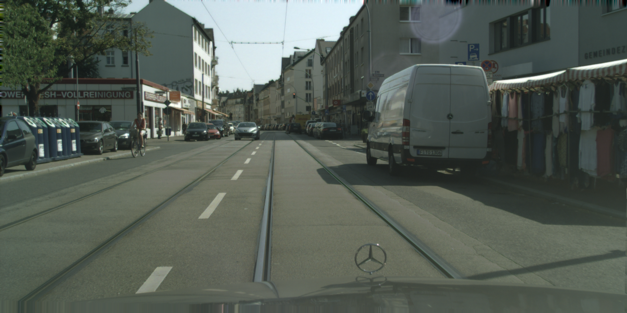
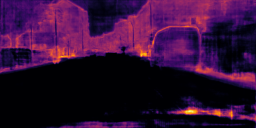
Figure 6: $\alpha$-maps of the semantic fusion gate depicted as heat maps (b) with respect to the original image (a). The brighter the pixel, the more important it is to the segmentation procedure. Sample image from the Cityscapes validation set.

Table 5: Comparative results in the Cityscapes testing set.

Method	Multi-scale	mIoU (%)
DeepLabV3+(dilated-ResNet-50) (Chen et al., 2018)		73.0
Dilated-ResNet-101 (Yu et al., 2017a)		75.7
DeepLabV3+(dilated-ResNet-101) (Chen et al., 2018)		76.5
Large Kernel Matters (Peng et al., 2017)		76.9
PSPNet(dilated-ResNet-101) (Zhao et al., 2017)	✓	78.4
PSANet(dilated-ResNet-101) (Zhao et al., 2018)	✓	80.1
Our(WideResNet-38)	✓	80.6

Table 6: Comparative results in the Mapillary Vistas validation set.

Method	mIoU (%)
FCN(WideResNet-38) (Wu et al., 2016)	41.1
FCN(WideResNet-38 + bcs) (Wu et al., 2016)	47.7
PSPNet(dilated-ResNet101) (Zhao et al., 2017)	49.7
Seamless (Porzi et al., 2019)	50.4
Ours(WideResNet-38)	52.3
Inplace-ABN (Rota Bulò et al., 2018)	53.1

Table 7: Comparative results in CamVid testing set.

Method	mIoU (%)
PSPNet(dilated-ResNet-101) (Zhao et al., 2017)	69.1
BiSetNet (Yu et al., 2018a)	68.7
Dilated ResNet-101 (Yu et al., 2017a)	65.3
BFP (Ding et al., 2019)	74.1
Ours(WideResNet-38)	75.1

Table 8: Comparative results in Pascal Context validation set.

Method	mIoU (%)
Dilated-ResNet-101 (Yu et al., 2017a)	42.6
RefineNet (Yu and Koltun, 2015)	47.3
PSPNet(dilated-ResNet101) (Zhao et al., 2017)	47.8
Ours(dilated-ResNet101)	48.1

Attention maps

The semantic fusion gate divides the input image pixels into two groups: Those related to the segmentation of boundary regions and those related to the segmentation of non-boundary regions. Figure 6 shows the $\alpha$-maps obtained from feeding two samples of the Cityscapes validation set to the semantic fusion gate, projected and visualized as heat maps. The brighter a region is in the figure, the more relevant it is to the task. In both of the illustrated examples, it is possible to observe that pixels located near the borders of objects are considered the brightest ones. Another noticeable point is that objects that are relatively smaller in a given scene appear to receive more attention from the boundary stream.

Boundary improvement

Figure 7 shows the results of how our model can improve semantic segmentation on boundary regions. To see a visual summary of the error of a semantic segmentation model, we take that model prediction from a given sample and subtract it from the ground truth. We perform these steps using DeepLabV3 and our proposed model to obtain Figure 7 and Figure 7, respectively. The results lead us to two conclusions: First, that our Y-model is capable of further refining segmentation borders when compared with other similar methods, and second that the gains reported in Figure 7 are obtained mainly through the improvement of boundary detection.

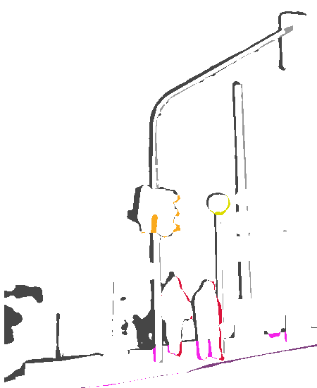
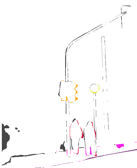
Figure 7: Comparison of the prediction segmentation error on the boundaries with respect to the ground truth: (a) DeepLabV3 (Chen et al., 2017), (b) our Y-model.

5.5 Discussion

Architecture

We explored the semantic boundary detection to improve the overall results of the semantic segmentation. For that, a semantic fusion gate was conceived to split semantic segmentation information between two convolutional network streams. Our Y-model structure works by capturing the different characteristics between the boundary and non-boundary pixels, and it was capable of combining both to perform the semantic segmentation task. This conclusion is backed by the results reported for the experiments carried out on different publicly available data sets that showed that our proposed model performs adequately. Tables 5, 7, and 8 clearly show that our Y-model was able to improve results when compared to other approaches in the literature. Even when the result achieved was not the best, the network was still competitive, as shown in Table 6. As shown in Figure 1, the current state-of-the-art models have issues to properly classify pixels on the image object boundary, and so we attribute our best results mainly to the improved representation and integration of the boundary features. Splitting segmentation and boundary detection allowed our proposed model for a better learning, since the Y-model focuses on representing the context of pixels independently of the borders.

Semantic fusion gate

Each stream (boundary and non-boundary) that composes our Y-model is responsible for specializing in different types of information for image segmentation. At the same time, however, these streams share enough information as to complement each other. This sharing is made possible through the semantic fusion gate, which we demonstrated to be an effective manner to fuse information from the two different sub-networks (streams). Table 2 showed that when using attention gating the results are generally better in comparison with other models that do not apply this merger by attention. The attention gate strategy showcases the importance of fusing features from the boundary and non-boundary streams in a witting way.

Integral crop

The data sets used in the experiments were burden by imbalance. This fact makes the less prevalent classes more difficult to learn. The proposed integral crop strategy aimed at reducing this effect by assigning weight values to each pixel by considering the inverse frequency of each class over the whole data set. This is so to hopefully select regions that best represents an uniform distribution of the data during the training stage. The results in Table 3 showed that this strategy could improve the segmentation results. Yet the use of integral images to compute each crop weight made the algorithm possible to run in linear time – mainly important as to avoid excessive pre-processing overhead during training.

6 Concluding remarks

Our proposed model has achieved results superior to the current state-of-the-art on most of the evaluated data sets. The promising results found ought to motivate other studies that explicitly explore the use of semantic boundaries for image segmentation in convolutional networks. We showed that explicitly considering semantic boundaries as part of the problem modeling may allow for a more satisfactory adjustment of the segmentation output with regards to the boundaries of objects in the scene. Our semantic fusion gate facilitated the learning of the two tasks simultaneously but separately, with each stream focusing on the appropriate information. It is important to note that the explicit representation of semantic boundaries increases the computational complexity of the model in memory requirements. So elaborating on more efficient forms of memory representation for semantic boundary can also be an important path for future research. Another possibly worthy investigation is on the use of other types of attention mechanisms, like the ones based on key, query, and value functions designed to work with attention gate, for example.

References

- Acuna et al. (2019) Acuna, D., Kar, A., Fidler, S., 2019. Devil is in the edges: Learning semantic boundaries from noisy annotations, in: IEEE Conference on Computer Vision and Pattern Recognition, pp. 11075–11083.
- Badrinarayanan et al. (2017) Badrinarayanan, V., Kendall, A., Cipolla, R., 2017. Segnet: A deep convolutional encoder-decoder architecture for image segmentation. IEEE transactions on Pattern Analysis and Machine Intelligence 39, 2481–2495.
- Bakas et al. (2017) Bakas, S., Akbari, H., Sotiras, A., Bilello, M., Rozycki, M., Kirby, J.S., Freymann, J.B., Farahani, K., Davatzikos, C., 2017. Advancing the cancer genome atlas glioma mri collections with expert segmentation labels and radiomic features. Scientific Data 4, 170117.
- Brostow et al. (2008) Brostow, G.J., Shotton, J., Fauqueur, J., Cipolla, R., 2008. Segmentation and recognition using structure from motion point clouds, in: European Conference on Computer Vision (ECCV), pp. 44–57.
- Chen et al. (2017) Chen, L.C., Papandreou, G., Schroff, F., Adam, H., 2017. Rethinking atrous convolution for semantic image segmentation. arXiv preprint arXiv:1706.05587 .
- Chen et al. (2018) Chen, L.C., Zhu, Y., Papandreou, G., Schroff, F., Adam, H., 2018. Encoder-decoder with atrous separable convolution for semantic image segmentation, in: European Conference on Computer Vision (ECCV), pp. 801–818.
- Cordts et al. (2016) Cordts, M., Omran, M., Ramos, S., Rehfeld, T., Enzweiler, M., Benenson, R., Franke, U., Roth, S., Schiele, B., 2016. The cityscapes dataset for semantic urban scene understanding, in: IEEE Conference on Computer Vision and Pattern Recognition (CVPR), pp. 3213–3223.
- Deng et al. (2009) Deng, J., Dong, W., Socher, R., Li, L.J., Li, K., Fei-Fei, L., 2009. ImageNet: A Large-Scale Hierarchical Image Database, in: IEEE Conference on Computer Vision and Pattern Recognition (CVPR), pp. 248–255.
- Ding et al. (2019) Ding, H., Jiang, X., Liu, A.Q., Thalmann, N.M., Wang, G., 2019. Boundary-aware feature propagation for scene segmentation, in: IEEE International Conference on Computer Vision, pp. 6819–6829.
- Fu et al. (2020) Fu, J., Liu, J., Jiang, J., Li, Y., Bao, Y., Lu, H., 2020. Scene segmentation with dual relation-aware attention network. IEEE Transactions on Neural Networks and Learning Systems , 1–14.
- Fu et al. (2019) Fu, J., Liu, J., Tian, H., Li, Y., Bao, Y., Fang, Z., Lu, H., 2019. Dual attention network for scene segmentation, in: IEEE Conference on Computer Vision and Pattern Recognition, pp. 3146–3154.
- He et al. (2016) He, K., Zhang, X., Ren, S., Sun, J., 2016. Deep residual learning for image recognition, in: IEEE Conference on Computer Vision and Pattern Recognition, pp. 770–778.
- Hu et al. (2019) Hu, Y., Chen, Y., Li, X., Feng, J., 2019. Dynamic feature fusion for semantic edge detection. Twenty-Eighth International Joint Conference on Artificial Intelligence (IJCAI-19) .
- Le and Duan (2020) Le, T., Duan, Y., 2020. Redn: A recursive encoder-decoder network for edge detection. IEEE Access 8, 90153–90164.
- Liang et al. (2015) Liang, X., Liu, S., Shen, X., Yang, J., Liu, L., Dong, J., Lin, L., Yan, S., 2015. Deep human parsing with active template regression. IEEE Transactions on Pattern Analysis and Machine Intelligence 37, 2402–2414.
- Liu et al. (2015) Liu, W., Rabinovich, A., Berg, A.C., 2015. Parsenet: Looking wider to see better. arXiv preprint arXiv:1506.04579 .
- Long et al. (2015) Long, J., Shelhamer, E., Darrell, T., 2015. Fully convolutional networks for semantic segmentation, in: IEEE Conference on Computer Vision and Pattern Recognition (CVPR), pp. 3431–3440.
- Ma et al. (2020) Ma, W., Gong, C., Xu, S., Zhang, X., 2020. Multi-scale spatial context-based semantic edge detection. Information Fusion 64, 238–251.
- Maggiori et al. (2017) Maggiori, E., Tarabalka, Y., Charpiat, G., Alliez, P., 2017. Can semantic labeling methods generalize to any city? the inria aerial image labeling benchmark, in: IEEE International Geoscience and Remote Sensing Symposium (IGARSS), IEEE. pp. 3226–3229.
- Mottaghi et al. (2014) Mottaghi, R., Chen, X., Liu, X., Cho, N.G., Lee, S.W., Fidler, S., Urtasun, R., Yuille, A., 2014. The role of context for object detection and semantic segmentation in the wild, in: IEEE Conference on Computer Vision and Pattern Recognition (CVPR), pp. 891–898.
- Narang et al. (2018) Narang, S., Diamos, G., Elsen, E., Micikevicius, P., Alben, J., Garcia, D., Ginsburg, B., Houston, M., Kuchaiev, O., Venkatesh, G., et al., 2018. Mixed precision training, in: International Conference on Learning Representations (ICLR).
- Neuhold et al. (2017) Neuhold, G., Ollmann, T., Rota Bulò, S., Kontschieder, P., 2017. The mapillary vistas dataset for semantic understanding of street scenes, in: International Conference on Computer Vision (ICCV), pp. 4990–4999.
- Peng et al. (2017) Peng, C., Zhang, X., Yu, G., Luo, G., Sun, J., 2017. Large kernel matters–improve semantic segmentation by global convolutional network, in: IEEE Conference on Computer Vision and Pattern Recognition, pp. 4353–4361.
- Perazzi et al. (2016) Perazzi, F., Pont-Tuset, J., McWilliams, B., Van Gool, L., Gross, M., Sorkine-Hornung, A., 2016. A benchmark dataset and evaluation methodology for video object segmentation, in: IEEE Conference on Computer Vision and Pattern Recognition, pp. 724–732.
- Porzi et al. (2019) Porzi, L., Bulo, S.R., Colovic, A., Kontschieder, P., 2019. Seamless scene segmentation, in: IEEE Conference on Computer Vision and Pattern Recognition, pp. 8277–8286.
- Ronneberger et al. (2015) Ronneberger, O., Fischer, P., Brox, T., 2015. U-net: Convolutional networks for biomedical image segmentation, in: International Conference on Medical Image Computing and Computer-assisted Intervention, Springer. pp. 234–241.
- Rota Bulò et al. (2018) Rota Bulò, S., Porzi, L., Kontschieder, P., 2018. In-place activated batchnorm for memory-optimized training of dnns, in: IEEE Conference on Computer Vision and Pattern Recognition, pp. 5639–5647.
- Santos et al. (2020) Santos, T.T., de Souza, L.L., dos Santos, A.A., Avila, S., 2020. Grape detection, segmentation, and tracking using deep neural networks and three-dimensional association. Computers and Electronics in Agriculture 170, 105247.
- Shrivastava et al. (2016) Shrivastava, A., Gupta, A., Girshick, R., 2016. Training region-based object detectors with online hard example mining, in: IEEE Conference on Computer Vision and Pattern Recognition, pp. 761–769.
- Takikawa et al. (2019) Takikawa, T., Acuna, D., Jampani, V., Fidler, S., 2019. Gated-scnn: Gated shape cnns for semantic segmentation, in: IEEE International Conference on Computer Vision, pp. 5229–5238.
- Wu et al. (2016) Wu, Z., Shen, C., Hengel, A.v.d., 2016. High-performance semantic segmentation using very deep fully convolutional networks. arXiv preprint arXiv:1604.04339 .
- Xie and Tu (2015) Xie, S., Tu, Z., 2015. Holistically-nested edge detection, in: IEEE international Conference on Computer Vision, pp. 1395–1403.
- Yang et al. (2018) Yang, M., Yu, K., Zhang, C., Li, Z., Yang, K., 2018. Denseaspp for semantic segmentation in street scenes, in: IEEE Conference on Computer Vision and Pattern Recognition, pp. 3684–3692.
- Yu et al. (2018a) Yu, C., Wang, J., Peng, C., Gao, C., Yu, G., Sang, N., 2018a. Bisenet: Bilateral segmentation network for real-time semantic segmentation, in: European conference on computer vision (ECCV), pp. 325–341.
- Yu and Koltun (2015) Yu, F., Koltun, V., 2015. Multi-scale context aggregation by dilated convolutions. arXiv preprint arXiv:1511.07122 .
- Yu et al. (2017a) Yu, F., Koltun, V., Funkhouser, T., 2017a. Dilated residual networks, in: IEEE Conference on Computer Vision and Pattern Recognition, pp. 472–480.
- Yu et al. (2017b) Yu, Z., Feng, C., Liu, M.Y., Ramalingam, S., 2017b. Casenet: Deep category-aware semantic edge detection, in: IEEE Conference on Computer Vision and Pattern Recognition, pp. 5964–5973.
- Yu et al. (2018b) Yu, Z., Liu, W., Zou, Y., Feng, C., Ramalingam, S., Vijaya Kumar, B., Kautz, J., 2018b. Simultaneous edge alignment and learning, in: European Conference on Computer Vision (ECCV), pp. 388–404.
- Zagoruyko and Komodakis (2016) Zagoruyko, S., Komodakis, N., 2016. Wide residual networks, in: Richard C. Wilson, E.R.H., Smith, W.A.P. (Eds.), British Machine Vision Conference (BMVC), BMVA Press. pp. 87.1–87.12.
- Zhang et al. (2018) Zhang, H., Dana, K., Shi, J., Zhang, Z., Wang, X., Tyagi, A., Agrawal, A., 2018. Context encoding for semantic segmentation, in: IEEE conference on Computer Vision and Pattern Recognition (CVPR), pp. 7151–7160.
- Zhao et al. (2017) Zhao, H., Shi, J., Qi, X., Wang, X., Jia, J., 2017. Pyramid scene parsing network, in: IEEE Conference on Computer Vision and Pattern Recognition (CVPR), pp. 2881–2890.
- Zhao et al. (2018) Zhao, H., Zhang, Y., Liu, S., Shi, J., Change Loy, C., Lin, D., Jia, J., 2018. Psanet: Point-wise spatial attention network for scene parsing, in: European Conference on Computer Vision (ECCV), pp. 267–283.
- Zhou et al. (2018) Zhou, Z., Siddiquee, M.M.R., Tajbakhsh, N., Liang, J., 2018. Unet++: A nested u-net architecture for medical image segmentation, in: Deep Learning in Medical Image Analysis and Multimodal Learning for Clinical Decision Support. Springer, pp. 3–11.
- Zhu et al. (2019) Zhu, Y., Sapra, K., Reda, F.A., Shih, K.J., Newsam, S., Tao, A., Catanzaro, B., 2019. Improving semantic segmentation via video propagation and label relaxation, in: IEEE Conference on Computer Vision and Pattern Recognition, pp. 8856–8865.