Two-Stage Sector Rotation Methodology Using Machine Learning and Deep Learning Techniques

Abstract

Market indicators such as CPI and GDP have been widely used over decades to identify the stage of business cycles and also investment attractiveness of sectors given market conditions. In this paper, we propose a two-stage methodology that consists of predicting ETF prices for each sector using market indicators and ranking sectors based on their predicted rate of returns. We initially start with choosing sector specific macroeconomic indicators and implement Recursive Feature Elimination (RFE) algorithm to select the most important features for each sector. Using our prediction tool, we implement different Recurrent Neural Networks (RNN) models to predict the future ETF prices for each sector. We then rank the sectors based on their predicted rate of returns. We select the best performing model by evaluating the annualized return, annualized Sharpe ratio, and Calmar ratio of the portfolios that includes the top four ranked sectors chosen by the model. We also test the robustness of the model performance with respect to lookback windows and look ahead windows. Our empirical results show that our methodology beats the equally weighted portfolio performance even in the long run. We also find that Echo State Networks (ESN) exhibits an outstanding performance compared to other models yet it is faster to implement compared to other RNN models.

Keywords: neural networks, echo state networks, recurrent neural networks, long short-term memory, gated recurrent units, feature selection, market indicators, exchange traded funds

1 Introduction

US economy has been following business cycles throughout the history. There are 11 business cycles identified by Natural Bureau of Economic Research since 1945 . Each business cycle has its own characteristics, yet there are similar patterns observed in each cycle. A typical business cycle starts with an economic growth until reaching a peak, and continues with an economic recession till attaining a trough. Market indicators have been used as the key determinants at identifying the stages of business cycles over decades. As a well-known model released by Merrill Lynch in 2004, Investment Clock uses growth (GDP) and inflation (CPI) factors to identify the four stages of the business cycle.

It has been observed that sector rotations occur at each stage of the business cycle. Depending on the phase of the cycle, investments on certain sector stocks tend to be more appealing. Sector rotation strategies have been built as a top-down approach to take advantage of the changing attractiveness of the sectors through business cycles. The stage of the business cycle is identified by analyzing macroeconomic indicators, and then investments are made based on the outperforming sectors for the chosen cycle. Numerous studies have shown that sector rotation strategies mostly beat the performance of the overall market.

Investment Clock is a very intuitive model, yet it only uses two factors to identify the status of the economy. In this paper, we benefit from a large number of common and sector specific macroeconomic indicators to identify the outperforming sectors as time progress. We aim at building a sector ranking model based on relative growth potential and investment attractiveness of eight major sectors: healthcare, technology, industrials, utilities, materials, energy, financial services and consumer discretionary. The ranking model will then be used for guiding private equity funds in the future in terms of sector targeting at particular points in time. We use public market information (ETFs) as a proxy for private market data because there is no available sector-wise private equity data, and the publicly available data for private equity funds is limited and scarce.

The contribution of this paper to the literature is two-fold. First, the existing literature is very limited on sector ranking models that are built using macroeconomic variables. In our paper, we consider a variety of sector-specific macroeconomic indicators for each sector and only add the most meaningful features into each sector prediction model. To the best of our knowledge, current literature only focuses on predicting sector rankings one month ahead. As our second contribution, we predict the sector rankings over different time horizons, and validate that our methodology provides comparable results even in the long run.

This paper is organized as follows: In Section 2, we go through the existing literature on market indicators. In Section 3, we describe our data set and the data preprocessing techniques that we implement for preparing data for modeling. Section 4 provides a technical background on the models that we implemented in this paper. We introduce our overall sector ranking methodology in Section 5. Section 6 starts with introducing the performance measures that are used in this paper. We also provide the backtesting results and the evolution of performance measures with increasing lookback window. Finally, we summarize our initial findings and explain our future extension plans in Section 7.

2 Literature Review

This paper contributes to two strands of literature: use of macroeconomic variables in asset return forecasting and building sector rotation methodologies. In Section 2.1, we introduce papers that use macroeconomic variables as predictors in asset return forecasting. Section 2.2 overviews the literature on tactical asset allocation using sector rotation strategies.

2.1 Macroeconomic Variables in Asset Return Forecasting

Numerous studies have attempted to identify the macroeconomic variables to be associated with the asset return prediction in different markets. Chen et al. [3] experimented with seven macroeconomic variables to explain the stock returns in US stock markets, and showed that industrial production, changes in risk premia, twist in yield curve, and inflation affect stock prices. On the other hand, they found that consumption and oil price do not have explanatory power on stock price behavior. In another study, Chen [2] found that default spread, term spread, one month T-bill rate, industrial production growth rate and dividend price ratio significantly impact stock prices. Clare and Thomson [9] analyzed the impact of 18 macroeconomic variables in UK stock markets, and concluded that oil price, retail price index, bank lending, and corporate default risk have impact on stock price movement. Mukherjee and Naka [25] identified the relationship between Japanese stock returns and exchange rate, inflation rate, money supply, real economic activity, long-term government bond rate, and call money rate. With a similar study in Norway stock markets, Gjerde and Saettem [12] ascertained the positive correlation of stock returns with oil price and real economic activity. They failed to show a strong correlation between stock returns and inflation. Chung and Shin [22] investigated the effect of macroeconomic variables on Korean stock prices, and revealed the significant impact of trade balance, foreign exchange rate, industrial production, and money supply on the stock prices. In another US market study, Flannery and Protopapadakis [10] investigated the impact of balance of trade, housing starts, employment, CPI, M1, and producer price index on equity trading volume. Ibrahim and Aziz [18] found that CPI and industrial production are positively related to Malaysian stock prices in the long-run. They also observed that stock prices have negative associations with exchange rate and money supply. Adam et al. [1] analyzed the short-term and the long-term effects of macroeconomic indicators on Ghanaian stock market indexes using Johansen’s multivariate cointegration test and innovation accounting techniques. Their experiments reveal that stock market indexes are significantly affected from inflation and exchange rates in the short-run, and from interest rate and inflation in the long-run. Singh et al. [29] found that exchange rate and GDP affects overall index returns in Taiwanese stock market. They showed that inflation rate, exchange rate, and money supply have negative associations with portfolios constructed using stocks of medium and large companies. Chong et al. [5] introduced a macroeconomic factor model, Eta model, using 18 macroeconomic variables to predict stock returns. In their model, they only included systematic variables such as unemployment rate, CPI, energy prices, and M2 money supply. They compared the performance of their model with that of Fama-French three-factor model. The experimental results show that their macroeconomic factor model outperforms the famous fundamental factor model. Chong and Phillips [7] implemented the Eta model on tactical asset allocation. They defined a metric called ECR (economic climare rating) that scores the impact of current economy on ETFs. The ratings change from one to five with five means economic environment is favorable for that ETF. Their strategy of using ETFs with 3, 4, and 5 ratings, and applying Mean-Variance Optimization outperformed benchmark models. Jare$\tilde{n}$o and Negrut [21] analyzed the impact of GDP, CPI, IPI, unemployment rate, and long-term interest rate on US stock prices, and found that all macroeconomic variables have significant effects except CPI. They further showed the positive association of GDP and IPI, and the negative association of unemployment rate and interest rate with stock prices. Misra [23] investigated the movement of Indian stock market using market indicators, and found a long-term impact of IPI, inflation, interest rate, gold price, exchange rate, foreign institutional investment, and money supply, and a short-term impact of inflation and money supply based on Vector Error Correction Model.

Paper	Year	Stock Market	Significant Market Indicators	Positive Association	Negative Association
[3]	1986	US	industrial production, twist in yield curve, changes in risk premia, inflation	-	-
[2]	1991	US	default spread,one month T-bill rate, term spread, dividend price ratio industrial production growth rate	-	-
[9]	1994	UK	oil price, retail price index, bank lending corporate default risk	-	-
[25]	1995	Japanese	inflation,real economic activity, money supply, call money rate long-term government bond rate	-	-
[12]	1999	Norway	oil price, real economic activity	oil price, real economic activity	-
[22]	1999	Korean	trade balance, foreign exchange rate industrial production, money supply	-	-
[10]	2002	US	trade balance, housing starts, employment, CPI, M1, PPI	-	-
[18]	2003	Malaysia	industrial production, CPI, money supply, exchange rate	industrial production, CPI	money supply, exchange rate
[1]	2008	Ghana	inflation, exchange rate, interest rate	-	-
[29]	2011	Taiwan	exchange rate, GDP, inflation rate, money supply	-	inflation rate, exchange rate, money supply
[21]	2016	US	GDP, IPI, unemployment rate, long-term interest rate	GDP, IPI	unemployment rate, interest rate
[23]	2018	Indian	IPI, inflation, interest rate, gold price, exchange rate, money supply, foreign institutional investment	-	-

Table 1: Literature on Macroeconomic Variables Used in Stock Return Forecasting

Table 1 summarizes the literature associated with the impact of macroeconomic variables on different markets. Although they are built using different market data, some market indicators have significant impacts on multiple markets such as inflation rate, CPI, IPI, and GDP. The observations indicate that unemployment rate, interest rate, and exchange rate are negatively impacting stock market movements, which is intuitively reasonable. Similarly, GDP, CPI, IPI, and oil price are positively associated with stock prices. The literature on macroeconomic variables solely focuses on the overall market stock prices. To the best of our knowledge, there is no existing literature that analyzes the sector-level impact of macroeconomic variables. In our paper, we first identify the possible sector-specific macroeconomic variables, and then investigate their impact on sector index returns based on US stock market.

2.2 Sector Rotation

A number of studies in the literature have constructed sector rotation strategies to outperform the performance of the overall market. There are two different research areas for sector rotation strategies. In the first research area, sector indexes are predicted using a variety of variables, and then sectors are ranked based on their predicted returns. In the second research field, the phase of the business cycles are detected, and investment strategies are developed based on outperforming stocks within the predicted phase.

The first research area focuses on building prediction models for sector indexes, and then rank sectors based on their returns. Moskowithz and Grinblatt [24] observed that investment momentum strategy of buying stocks from winning industries and selling stocks from losing industries is profitable. In their model, they rank 20 US sector stocks based on their six month historical stock prices, and then invest in top 30 percent of stocks while shorting low 30 percent of stocks. Chong and Phillips [6] implemented the macroeconomic Eta model on sector rotation strategies. The model is calibrated using three-years data with 18 macroeconomic factors to predict ETF sector indexes. They selected sectors based on the criteria of 95 percent or higher $R^{2}$ value in Eta model, and applied Mean Variance Optimization (MVO) to construct the portfolio. By following long-only strategy and re-balancing the portfolio semiannually, they found that their strategy outperforms benchmark portfolios. Gao and Ren [11] employed principal component regression to predict future sector indexes in Shanghai Security Market. They calibrated their model using four years data, and predicted the sector returns for the following week. Their strategy of buying the top sector index and selling the lowest sector index achieved better average weekly returns in comparison to market composite index. Zhu et al. [31] applied explainable AI models such as linear regression, ridge regression and random forest using five macroeconomic indicators (growth factor, inflation factor, rate factor, credit factors, and exchange factor), and predicted the monthly sector index returns in Chinese stock market. The models are calibrated using two years data, and the next month returns are predicted. They experimented with one month, six months, and one year lagged indicators, and implemented PCA and feature importance with random forest on lagged indicators. They selected top five sectors based on their rate of return, and their monthly re-balanced portfolio outperformed equally-weighted index portfolio.

There also exists studies on prediction models for the phase of the business cycle. The investment strategies are built based on the performance of sectors within predicted stage of the business cycle. Greetham and Hartnett [13] introduced Investment Clock in 2004 in order to identify four stages of a business cycle: recovery, overheat, stagflation, and reflation. Different stages of the business cycle are detected based on the trend of growth (GDP) and inflation (CPI). They observed that consumer discretionary, telecom, and technology stocks perform well during recovery; whereas technology, industrials, oil and gas sector stocks perform the best during overheat. Outperforming stocks in stagflation phase are the stocks from oil and gas, pharmaceuticals, and utilities sectors. Consumer staples, financials, and consumer discretionary stock prices are tend to be high over reflation period. Raffinot and Benoit [26] implemented random forest and boosting algorithms to predict the turning points in the economy based on the deviation of real GDP from its trend. Their model consists of two types of turning points: acceleration and slowdown. According to their investment strategy, they invest 80% of their money to equities, and the remaining 20% to the bonds when acceleration is expected in the economy. Otherwise, 40% of the portfolio will belong to equities, and the rest will be invested in bonds. Sauer [28] divided the status of economy into four cases based on the regimes observed in GDP: high rising, high falling, low rising, and low falling. Since GDP is reported quarterly, the data is transformed into monthly frequency using monthly industrial production as an indicator. Two independent random forest models are developed to predict two-level regime (high vs low) and two-level momentum (rising vs. falling). By excluding cyclical sectors in low falling regime, they managed to outperform equally-weighted benchmark. Wang et al [30] divided economy into four regimes based on GDP year over year change and 10 year treasury bond yield. They implement k-Nearest Neighbors algorithm to predict the status of the economy based on macroeconomic factors. Furthermore, they employed post-Lasso regression for all sector indexes in each economic regime to predict the next month sector returns using the related sector historical return data. Based on the status of the economy, corresponding post-Lasso models are used to predict sector returns, and the strategy of longing top 20% sector indexes and shorting the bottom 20% of sector indexes is employed. Their investment strategy mostly outperformed the equally-weighted benchmark.

In our paper, we implement ML & DL models to predict sector index returns using sector-specific macroeconomic indicators. We then rank the sectors based on their predicted rate of returns, and select top four ranked sectors for long-only strategy. Our paper belongs to the first research area, yet the existing literature focuses only on the one month ahead predictions. We extend our prediction horizon up to two years, and evaluate the robustness of our methodology by experimenting with different prediction horizons.

3 Data

To compare the performance of different sectors, we utilize iShares ETF prices for eight major sectors: healthcare (IYH), energy (IYE), utilities (IDU), finance (IYG), technology (IYW), materials (IYM), industrials (IYJ), and consumer goods (IYK). Our dataset consists of ETF prices for each sector from July 14, 2000 to Nov 10, 2019. As we use the market calendar of NYSE, we obtain 4,862 daily adjusted close prices for each ETF. We utilize yfinance python library to download the data. In this paper, we mostly experiment with monthly data. Therefore, we obtain 233 monthly adjusted close prices.

Macroeconomic variables that we consider in this study comes from a variety of resources. Appendix A provides the tables of macroeconomic variables for each sector together with their resources and data frequencies. Table A7 gives the list of macroeconomic variables that are commonly used as input for each sector model. These macroeconomic variables include gross domestic product (GDP), unemployment rate, consumer price index (CPI), 30-year fixed rate mortgage rate, and federal funds rate. As it is seen, macroeconomic variables are reported on different time frequency basis varying from daily to annually. Thus, we implement linear interpolation to obtain monthly observations for each macroeconomic variable. After the interpolation, the dataset of macroeconomic variables align with sector ETF prices.

For each sector, we define the relevant macroeconomic variables, but using too many features leads to an increase in the model complexity, and it may further cause multicollinearity between variables and model overfitting. Recursive Feature Elimination (RFE) (Guyon et al. [14]) algorithm is implemented to avoid these problems and to obtain the most important features for each sector. RFE is a backward selection algorithm, which recursively fits a machine learning model using all available features, and calculates the importance of each feature within the model. The algorithm eliminates the least important features at each iteration until the predetermined number of features are obtained. The relative importance of each feature is measured by the average decrease in node impurity caused by that feature. In this paper, we employ random forest regression as a sub-routine machine learning model, and we select top four ranked features as the final set of features.

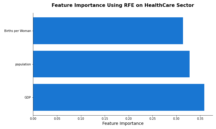
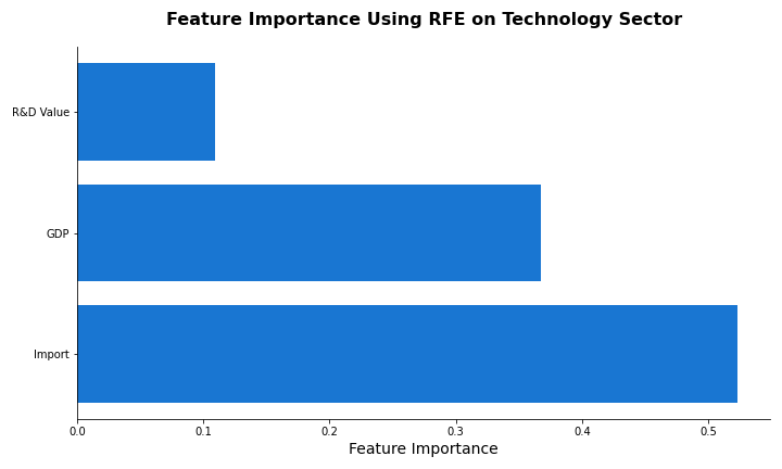
Figure 1: Feature Importance Using RFE on Different Sectors

Figure 1 provides feature importance plots obtained using RFE algorithm for finance and technology sectors. According to the plots, GDP is a very significant feature while predicting sector index prices. Finance sector ETF prices are highly affected by unemployment rate and trade balance % of GDP. R&D value and import are also key drivers for technology sector index prices which is expected by intuition.

4 Preliminaries

In this section, we provide a background on the existing machine learning and deep learning models that we implement within our overall model framework. These models are ridge regression, long short-term memory (LSTM), gated recurrent unit (GRU), and echo state networks (ESN), respectively.

4.1 Ridge Regression

Ridge regression is a type of regularized regression proposed by Hoerl and Kennerd [16],[17] to control the high variance of estimates due to the multicollinearity between the features. We apply ridge regression as our benchmark model because it is commonly used in industry. Ridge regression estimates $\beta$ regression coefficients within the formula:

$$y=X\beta+\epsilon,$$

where $X\in\mathbb{R}^{n\times p}$ is the predictor matrix, $y\in\mathbb{R}^{n}$ is the response vector, and $\epsilon\in\mathbb{R}^{n}$ is residuals. Although very similar to linear regression, ridge regression adds $L_{2}$ penalty term on the coefficients in the objective function, and controls the strength of penalty with $\lambda$ tuning parameter. In the existence of multicollinearity, the variance of the estimates will be high. By adding penalty, ridge regression shrinks the regression coefficients towards zero and controls the variance of estimates. Equation 1 provides the analytical solution for $\beta$ coefficients.

$$\beta_{ridge}=\arg\min_{\beta}||y-X\beta||_{2}^{2}+\lambda||\beta||_{2}^{2}=(X^{\intercal}X+\lambda I)^{-1}X^{\intercal}y$$ (1)

In comparison to linear regression where there is an uncertainty on non-singularity of $X^{\intercal}X$, $X^{\intercal}X+\lambda I$ in ridge regression is a non-singular and hence an invertible matrix that stabilizes the estimates. Despite the certain advantages of ridge regression over linear regression, we expect that the performance of RNNs will be superior to that of ridge regression because the latter one do not consider the temporal patterns within the data.

4.2 Recurrent Neural Networks (RNNs)

Vanilla feedforward neural networks (FNNs) do not consider any temporal dependencies within the data because they rely on the assumption of independence between inputs and outputs. They are not able to understand the dependencies within the time-series data. On the other hand, recurrent neural networks (RNNs) (Rumelhart et al. [27]) carry a memory through time steps of the data to remember the temporal dynamic behavior of the data. RNNs can learn temporal dependencies within the data using their hidden units $h_{t}$. Equation 2 shows the general structure of the relationship between hidden units, where $f$ represents a non-linear activation function. At each time step, the values of hidden units are calculated based on a non-linear function $f$, and $f$ takes the values of hidden units at previous time steps as input together with the input $x_{t}$ from the current time step.

$$h_{t}=f(h_{t-1},x_{t})$$ (2)

RNNs are trained using Backpropagation Through Time (BPTT) algorithm. Hidden units in the same layer share the same weight matrices and bias vectors. BPTT algorithm calculates the gradient of chosen loss function with respect to these weight matrices and bias vectors. When the sequence of the data is long, vanishing gradient problem may occur. In the case of vanishing gradients, weight matrices and bias vectors are not updated enough and learning stops. Although RNNs are good at capturing short-term dependencies, they are vulnerable to failure at memorizing longer term relationships. Gated recurrent neural networks has been built to address the vanishing gradients problem and to understand long-term dependencies within the data. In this study, we benefit from two most popular gated RNNs: Long Short-Term Memory (LSTM) and Gated Recurrent Units (GRUs).

4.3 Long Short-Term Memory (LSTM)

Long Short-Term Memory (LSTM) (Hochreiter and Schmidhuber [15]) is a type of RNNs, where $f$ non-linear activation function in Equation 2 is replaced by an LSTM memory cell. Each memory cell controls the flow of memory cell state $c_{t}$ by adding three gates: forget gate $f_{t}$, input gate $i_{t}$, and output gate $o_{t}$. Figure 2 illustrates a typical LSTM memory cell.

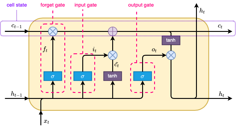
Figure 2: LSTM Memory Cell

As it is seen in Figure 2, each input gate takes hidden state from previous time step $h_{t-1}$ and new information from current time step $x_{t}$ as input. Sigmoid activation function $f(x)=\frac{1}{1+e^{-x}}$ is then used to control the level of information flow in each gate (Equations 3, 4, and 7). While forget gate $f_{t}$ determines the amount of existing memory $c_{t-1}$ to forget, input gate $i_{t}$ decides on how much to add a new memory from $\tilde{c_{t}}$ into the current cell state (Equation 6). Output gate $o_{t}$ calculates which parts of cell state $c_{t}$ to keep in hidden state $h_{t}$.

$$f_{t} =\sigma\left(W_{f}\cdot h_{t-1}+U_{f}\cdot x_{t}+b_{f}\right)$$ (3)

$$i_{t} =\sigma\left(W_{i}\cdot h_{t-1}+U_{i}\cdot x_{t}+b_{i}\right)$$ (4)

$$\tilde{c_{t}} =tanh\left(W_{c}\cdot h_{t-1}+U_{c}\cdot x_{t}+b_{c}\right)$$ (5)

$$c_{t} =f_{t}\circ c_{t-1}+i_{t}\circ\tilde{c_{t}}$$ (6)

$$o_{t} =\sigma\left(W_{o}\cdot h_{t-1}+U_{o}\cdot x_{t}+b_{o}\right)$$ (7)

$$h_{t} =o_{t}\circ tanh(c_{t})$$ (8)

LSTM memory cell flow is regularized by sigmoid ($\sigma$) and hyperbolic tangent ($tanh$) activation functions. Since $\sigma$ takes values between 0 and 1, and $tanh$ takes values between -1 and 1, the flow of information is controlled by bounded non-linear functions. Therefore, BPTT algorithm works smoothly without observing vanishing gradients problem quickly.

4.4 Gated Recurrent Unit (GRU)

GRU is a more recent version of gated RNNs, which is introduced by Cho et al. [4] in 2014. Similar to LSTM, $f$ function in Equation 2 is replaced by a GRU unit. Each GRU unit consists of two gates: update gate $z_{t}$, and reset gate $r_{t}$. As opposed to LSTM memory cells, GRU units do not have a separate cell state. All information flow through hidden states $h_{t}$. In addition, forget gate and input gate in LSTM memory cells are represented with a single update gate $z_{t}$ in GRU units. Figure 3 illustrates a typical GRU unit.

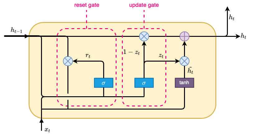
Figure 3: GRU Memory Cell

Equations 9 and 10 shows that each gate takes the previous hidden state $h_{t-1}$ and the new information from the current time step $x_{t}$ as input, and apply a sigmoid activation function to control the information flow. Reset gate decides on the extent to remember the previous information $h_{t}$. Update gate $z_{t}$ determines the level of information to forget from the previous hidden state $h_{t-1}$ and the level of information to add from the new candidate hidden state $\tilde{h_{t}}$ (Equation 12).

$$z_{t} =\sigma\left(W_{z}\cdot h_{t-1}+U_{z}\cdot x_{t}+b_{z}\right)$$ (9)

$$r_{t} =\sigma\left(W_{r}\cdot h_{t-1}+U_{r}\cdot x_{t}+b_{r}\right)$$ (10)

$$\tilde{h_{t}} =tanh\left(W_{h}\cdot(r_{t}\circ h_{t-1})+U_{h}\cdot x_{t}+b_{h}\right)$$ (11)

$$h_{t} =(1-z_{t})\circ h_{t-1}+z_{t}\circ\tilde{h_{t}}$$ (12)

GRU unit is also regularized by sigmoid and $tanh$ activation functions. Therefore, BPTT algorithm works smoothly and avoids vanishing gradients problem to a large extent. In their empirical study, Chung et al. [8] compared the performance of LSTM and GRU, and they observed that both models are comparable to each other. GRU is faster than LSTM because it has fewer parameters in terms of number of gates and inexistence of the cell state. However, fewer number of parameters in GRU may also result in a decrease in the expressability. Since our data is limited, we expect that GRU model will be more suitable for our study compared to LSTM model.

4.5 Echo State Networks (ESN)

Echo State Networks (ESNs) (Jaeger [19]) are also a type of RNNs, but they address the vanishing gradients problem by employing a reservoir computing framework instead of gates. The model consists of three weight matrices: weights from input layer to reservoir ($W_{in}$), weights within reservoir ($W$), and weights from reservoir to output layer ($W_{out}$). $W_{in}$ and $W$ are randomly initialized, but they remain fixed throughout the training. $W_{out}$ is the only weight matrix trained to capture the temporal dynamics of the data. Figure 4 illustrates the general architecture of ESNs.

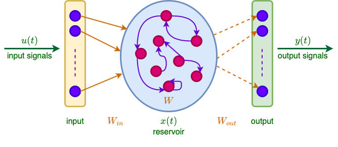
Figure 4: Echo State Networks

The algorithm consists of two steps. In the first step, the input signals $u(t)$ are converted into high-dimensional non-linear embeddings $x(t)$ through reservoir as in Equation 13. The non-linearity of $x(t)$ comes from the function $f$, that is a non-linear activation function such as sigmoid and $tanh$. The relationship between $x(t)$ and output signals $y(t)$ are then calculated based on Equation 14. Function $g$ is usually taken as linear function. Hence, a linear regression algorithm is trained to find $W_{out}$. Equations 13 and 14 are taken from Jaeger et al. [20] because leaky integrators and tunable hyperparameters are included in the formulation.

$$x(t+1) =(1-\alpha)x(t)+f(s_{in}W_{in}u(t+1)+(\rho W)x(t))$$ (13)

$$y(t+1) =g(W_{out}[x(t);u(t)])$$ (14)

In Equation 13, $\alpha$, $s_{in}$, and $\rho$ represent leaking rate, input scaling, and spectral radius, respectively. Leaking rate $\alpha$ determines the speed of the changes in $x(t)$. Input scaling $s_{in}$ is used to scale the weight matrix $W_{in}$. Spectral radius $\rho$ is the maximum absolute eigenvalue of the weight matrix $W$. The weight matrix $W$ is scaled by $\rho$, and larger spectral radius is used to consider longer memory. These hyperparameters together with reservoir size $N$ should be tuned in order to obtain the best model given the data.

Despite traditional RNNs, ESNs do not suffer from vanishing gradients problems as ESNs are not trained through BPTT. In addition, training of ESNs are faster compared to other RNNs because only a regression-like algorithm is used to train the model. Considering these two advantages, we expect that the performance of ESNs will be superior compared to the performance of other models we implement in this study.

5 Proposed Methodology

In this section, we introduce our overall methodology for ranking sectors based on the market environment. Figure 5 illustrates our overall methodology diagram. As in Figure 5, our methodology consists of two stages: prediction tool and ranking sector based on index returns. The prediction tool is applied on each sector independently. For each sector, we take common and sector specific macroeconomic indicators as input, and index prices as output. We employ Recursive Feature Elimination (RFE) on these variables, and pick the most important variables for each sector. Using selected features, we then predict the future sector index prices by employing the models from Section 4. We implement our prediction tool for each sector, and obtain the predictions for the future sector index prices. In the second stage, we calculate future sector index returns using predicted sector index prices. Finally, we rank the sectors based on their predicted rate of returns.

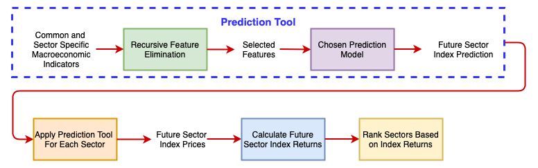
Figure 5: Overall Ranking Methodology

6 Experimental Results

To evaluate the ability of our methodology on sector ranking that is introduced in Section 5, we conduct experiments to predict near-term, mid-term, and long-term rankings of sectors. In this section, we show our results for each prediction time horizon and investigate the behavior of different models with the change of lookback window. We also build a strategy for choosing the best performing model and lookback window.

We use the same values for the hyperparameters through all prediction models to analyze the robustness of the models across different look ahead periods. These values are obtained based on our earlier experiments. We use $\alpha=10$ for all ridge regression models. LSTM model is built using three hidden layers. The layers consist of 16, 256, and 64 hidden units, respectively. Our experiments show that relu activation function performs the best for all hidden layers. During the training, we try to minimize Root of Mean Squared Error (RMSE) using Adam optimizer with learning rate$=0.0001$ and decay$=1e-7$. We train the models for 1,000 epochs, and monitor the value of RMSE during the training for early stopping. The layout of GRU is similar to that of LSTM. We again use three hidden layers with relu activation function. Each hidden layer consists of 32, 256, and 64 hidden units, respectively. We train our models for 500 epochs, and allow for early stopping. ESN model is built using 100 reservoir units. The leaking rate, spectral radius, and reservoir density are set to 0.5, 1, and 0.5, respectively. For the regression routine of ESN model, we use ridge regression with $\alpha=1$. Finally, the transient time is chosen to be zero. It is important to note that these hyperparameters are chosen based on our preliminary experiments. We plan to integrate hyperparameter optimization techniques into our methodology as a future work.

After running all models with a variety of lookback windows for each prediction horizon, we calculate the returns of each sector. In order to backtest the performance of different models on identifying sector rankings, we select top four sectors based on returns at each time step, and form an equally weighted portfolio based on the returns predicted through each model. We then compare the performance of the models with respect to each other and the benchmark portfolio. The benchmark portfolio is formed by all sector ETFs, and each sector shares an equal weight within the portfolio. As performance measure, we use annualized returns, annualized Sharpe ratio, and annualized Calmar ratio.

6.1 Performance Metrics

As stated earlier, we use annualized return, annualized Sharpe ratio, and annualized Calmar ratio to evaluate the performance of portfolios that are created by using different models and benchmark portfolio. In this section, we briefly explain what they are.

Annualized rate of return is the annual return of a portfolio over a given period of time. Using annualized rate of return, an investor can compare the performance of portfolios that are invested for different duration. Equation 15 shows that annualized return is calculated as the geometric average of the returns over a given time horizon. Return in Equation 15 is the percentage change of the price over given period. n indicates the period frequency within a year, and N stands for the total number of periods within given time horizon. In this paper, we mostly use n$=12$ because we consider monthly returns.

$$\text{Annualized Return}=\left(\left(1+\text{Return}\right)^{\text{n}/\text{N}}-1\right)\times 100$$ (15)

Annualized rate of return allows comparison of different portfolios, but it doesn’t take into account the risk related to the investment. Sharpe ratio, introduced by William Sharpe in 1966, is a risk-adjusted performance metric, and it shows the excess return of the portfolio per unit of risk. Equation 16 provides the overall formula of Sharpe Ratio, where RF is the risk-free rate. Therefore, the numerator represents the average excess return of the portfolio with respect to a risk-free asset, and the denominator is the standard deviation of the excess return of the portfolio. In this paper, we use risk-free rate is equal to zero for simplicity.

$$\text{Sharpe Ratio}=\frac{\mathbb{E}\left[\text{Return}-\text{RF}\right]}{\sigma}$$ (16)

To compare the performance of the portfolios with different duration, we calculate the annualized Sharpe Ratio in Equation 17. Annualized Sharpe ratio is calculated as the multiplication of Sharpe ratio from Equation 16 and the square-root of the period frequency within a year.

$$\text{Annualized Sharpe Ratio}=\text{Sharpe Ratio}\times\sqrt{n}$$ (17)

Calmar ratio is another risk-adjusted performance metric that we considered in this paper. Instead of the standard deviation of excess returns, Calmar ratio uses maximum drawdown as the risk measure. Maximum drawdown is an indicatior of the largest loss that an investor can suffer. It is calculated as the maximum loss incurred by investing at the peak price and selling at the trough price. Equation 18 show that Calmar ratio is simply formulated as the annualized return from Equation 15 over the maximum drawdown.

$$\text{Calmar ratio}=\frac{\text{Annualized Return}}{\text{Maximum Drawdown}}$$ (18)

When evaluating the models in the following sections, we seek for attaining the maximum values for these three performance measures. If each performance indicates a different model or different lookback window, we then select the model and lookback window providing a balance between performance metrics.

6.2 Near-Term Results

We predict one month ahead and three months ahead sector rankings to show how our model performs for near-term sector rankings.

Lookback Window	Model	In-Sample Performance			Out-of-Sample Performance
(Years)		Annualized Return	Sharpe Ratio	Calmar Ratio	Annualized Return	Sharpe Ratio	Calmar Ratio
Benchmark		8.81%	0.660	0.175	13.60%	1.200	0.990
0.5	Ridge	13.19%	0.858	0.318	10.22%	0.953	0.633
	LSTM	17.70%	0.898	0.479	10.42%	1.212	0.677
	GRU	15.73%	0.934	0.417	10.38%	1.148	0.643
	ESN	17.89%	1.239	0.474	13.70%	1.226	1.127
1	Ridge	13.32%	1.224	0.365	12.88%	0.984	1.220
	LSTM	20.20%	1.271	0.602	13.96%	1.384	1.386
	GRU	17.05%	1.080	0.470	11.75%	1.213	0.773
	ESN	21.53%	1.034	0.689	12.05%	1.457	0.809
1.5	Ridge	14.68%	0.960	0.431	10.34%	1.074	0.796
	LSTM	19.66%	1.198	0.567	14.08%	1.332	1.063
	GRU	14.97%	0.840	0.343	9.55%	1.091	0.522
	ESN	22.38%	1.286	0.757	15.46%	1.517	1.028
2	Ridge	16.06%	1.126	0.450	13.02%	1.169	0.970
	LSTM	20.98%	1.017	0.611	12.74%	1.381	0.652
	GRU	17.34%	1.048	0.486	11.70%	1.194	0.813
	ESN	24.25%	1.330	0.781	16.10%	1.639	1.070
2.5	Ridge	16.56%	1.040	0.483	11.52%	1.218	0.903
	LSTM	20.28%	1.111	0.658	13.04%	1.411	0.984
	GRU	17.19%	0.965	0.401	10.26%	1.210	0.784
	ESN	24.72%	1.072	0.794	12.86%	1.643	0.789
3	Ridge	16.93%	1.235	0.498	14.15%	1.224	1.219
	LSTM	19.24%	1.466	0.610	17.83%	1.342	1.601
	GRU	10.41%	0.931	0.193	10.49%	0.775	0.602
	ESN	25.08%	1.022	0.862	12.70%	1.702	0.777

Table 2: Next Month Prediction Results - Performance Measures

Table 2 provides the performance of the portfolios formed based on different models and different lookback windows and compares these measures with that of benchmark portfolio for both training data and testing data. Results show that all models form superior portfolios in comparison to the benchmark portfolio under three performance metrics. For each lookback window, ESN provides the best annualized return and LSTM follows ESN. There is a similar pattern for annualized Calmar ratio. However, there is no clear pattern for annualized Sharpe ratio. For half of the lookback windows, LSTM performs the best, and ESN performs the best for other lookback horizons. Out-of-sample results show that ESN and LSTM based portfolios perform superior most of the time in terms of annualized returns. Similarly, annualized Sharpe ratios for these two models are superior to that of benchmark portfolio for each lookback window. ESN performs better than LSTM regarding annualized Sharpe ratio. There is no clear pattern for annualized Calmar ratio for the testing horizon.

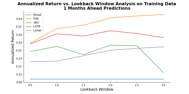
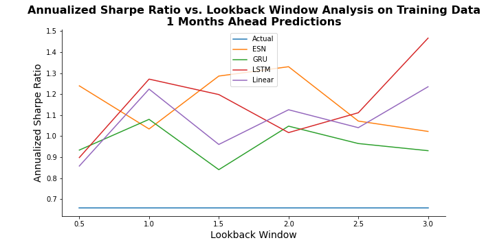
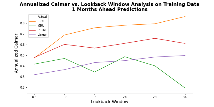
Figure 6: Comparison of Different Lookback Windows and Different Models for Next Month Prediction

Figure 6 illustrates how performance of different models change based on different lookback windows. Here, lookback window equals to 0.5 means that we use the last six months values of macroeconomic variables to predict a month ahead sector rankings. Plots show that portfolios formed based on all four models perform better than our benchmark portfolio during training horizon. Our results show that for annualized return and annualized Calmar ratio, ESN model creates a portfolio that is superior to other portfolios for all lookback windows, and LSTM follows ESN. There is no generic pattern for each model, but in general the annualized returns and annualized Calmar ratios increase as we use more historical data for predictions. For annualized Sharpe ratio, there is no strong correlation between lookback window and model performance. The best annualized Sharpe ratio is attained with three years historical data and LSTM model. Based on the performance measure criteria chosen, different models and different lookback windows are chosen for the final prediction model. If our priority is the annualized return or annualized Calmar ratio, then ESN with three years of historical data performs the best despite LSTM with three years of historical data is chosen for annualized Sharpe ratio. However, ESN with three years data do not give a nice annualized Sharpe ratio, and LSTM is not the best choice for the other performance metrics.

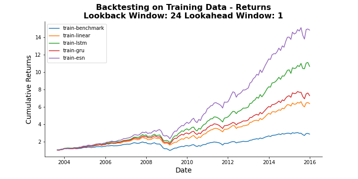
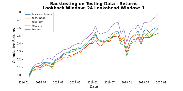
Figure 7: Backtesting Performance for Next Month Prediction Models (Two Years Lookback Window)

To obtain nice results for each performance metric without sacrificing, we check the second best models for each performance metric. We observe that ESN with two years of historical data provides satisfactory performance during training horizon. Figure 7 illustrates the backtesting results for different models with two years of historical data. All models exhibit superior performance in terms of cumulative returns during training horizon. ESN performs the best as expected. During the testing horizon, the performance of ESN is superior to the benchmark portfolio and other models. However, other models mostly underperform benchmark portfolio during testing period. There could be potential reasons for the changing performance during testing horizon. First, the benchmark portfolio performs better during testing period in comparison to training period. A thorough hyperparameter tuning could enhance the performance of other models during the testing period. Appendix B.1 provides the performance metric plots for testing period and backtesting plots based on other lookback windows.

Lookback Window	Model	In-Sample Performance			Out-of-Sample Performance
(Years)		Annualized Return	Sharpe Ratio	Calmar Ratio	Annualized Return	Sharpe Ratio	Calmar Ratio
Benchmark		7.93%	0.589	0.157	13.60%	1.200	0.990
1	Ridge	11.06%	1.060	0.268	12.01%	0.826	1.057
	LSTM	17.70%	1.051	0.504	12.93%	1.205	0.837
	GRU	7.11%	1.163	0.127	12.86%	0.546	1.087
	ESN	18.95%	1.285	0.533	13.90%	1.253	1.272
2	Ridge	15.48%	1.138	0.413	12.35%	1.094	1.125
	LSTM	21.16%	1.417	0.643	16.59%	1.418	1.268
	GRU	11.92%	1.091	0.246	11.51%	0.848	0.836
	ESN	23.05%	1.397	0.738	16.02%	1.534	1.450
3	Ridge	17.40%	1.172	0.508	13.08%	1.212	1.501
	LSTM	19.90%	1.301	0.571	15.38%	1.321	1.389
	GRU	13.45%	1.322	0.344	15.51%	0.960	1.169
	ESN	24.93%	1.527	0.768	16.46%	1.635	1.958
4	Ridge	16.99%	1.111	0.496	11.65%	1.192	1.149
	LSTM	20.23%	1.177	0.578	15.44%	1.321	1.008
	GRU	10.02%	0.923	0.218	11.23%	0.696	0.614
	ESN	27.22%	1.574	0.894	17.58%	1.746	1.575

Table 3: Three Months Ahead Prediction Results - Performance Measures

In Table 3, performance of different models based on different lookback windows are provided for three months ahead predictions. The results show that annualized returns obtained during training period are higher than that of benchmark portfolio for all models. As in Table 2, portfolios based on ESN models provide the highest annualized returns during training period. The pattern is similar both for annualized Sharpe ratio and annualized Calmar ratio during training period. During the testing period, ESN and LSTM models attain better annualized returns compared to the benchmark and other two models. The best performance in terms of annualized Sharpe ratio and annualized Calmar ratio is attained also by ESN and LSTM models.

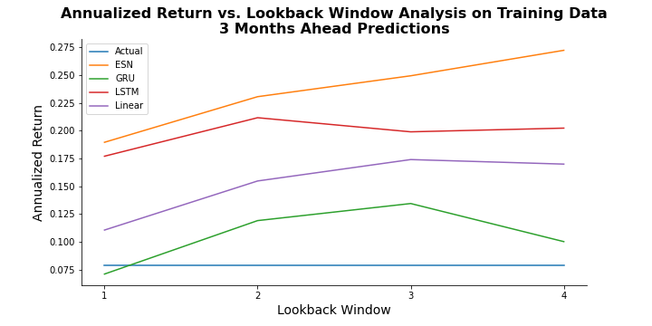
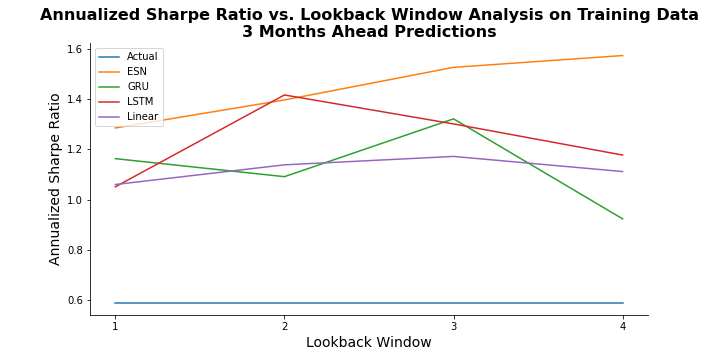
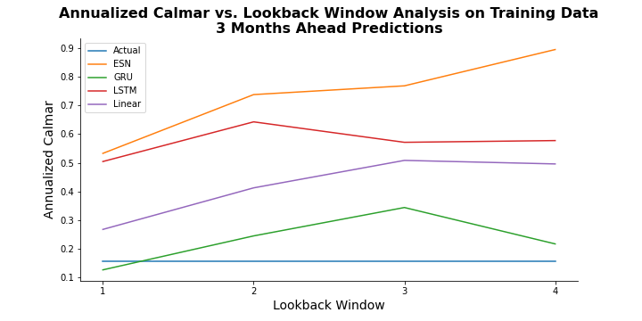
Figure 8: Comparison of Different Lookback Windows and Different Models for Three Months Ahead Prediction

Figure 8 illustrates the behavior of different models with different lookback windows for three months ahead predictions. For each performance metric plot, it is seen that ESN model performance increases as more historical data included in the model. For LSTM model, the performance increases from one year to two years, but then it decreases as we include more historical data. Similarly, GRU and ridge model performances increase from one year to three years but then decreases. For all performance metrics, ESN with four years of historical data provides the best performance.

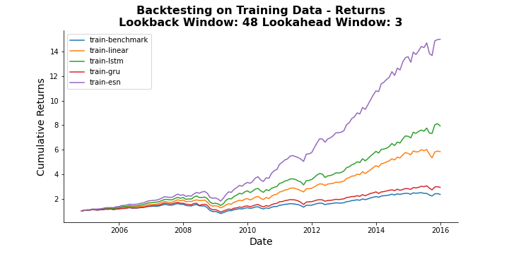
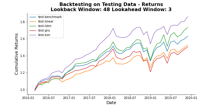
Figure 9: Backtesting Performance for Three Months Ahead Prediction Models (Four Years Lookback Window)

Figure 9 shows the backtesting results for the models that use four years of historical data. During training period, portfolios formed by all models outperform the benchmark portfolio. ESN performs the best, and LSTM follows ESN. Testing period cumulative returns show that ESN ourperforms all the models and also benchmark period. LSTM model also provides better cumulative returns over testing period in comparison to benchmark portfolio. Appendix B.2 consists of the performance metric plots for testing period and also the backtesting results for other lookback windows.

6.3 Medium-Term Results

We predict six months ahead and one year ahead sector rankings to show how our methodology works for medium-term sector rankings.

Lookback Window	Model	In-Sample Performance			Out-of-Sample Performance
(Years)		Annualized Return	Sharpe Ratio	Calmar Ratio	Annualized Return	Sharpe Ratio	Calmar Ratio
Benchmark		7.24%	0.544	0.144	13.60%	1.200	0.990
1	Ridge	12.95%	0.760	0.302	8.17%	0.885	0.562
	LSTM	19.19%	1.460	0.577	16.24%	1.256	1.386
	GRU	9.05%	1.172	0.159	13.26%	0.653	1.090
	ESN	17.88%	1.434	0.482	16.73%	1.191	1.371
2	Ridge	13.59%	1.083	0.361	11.60%	0.984	1.117
	LSTM	18.42%	1.415	0.514	16.50%	1.251	1.247
	GRU	9.39%	1.183	0.201	12.61%	0.684	1.500
	ESN	20.61%	1.477	0.584	16.01%	1.355	1.411
3	Ridge	15.29%	1.352	0.402	14.84%	1.077	1.406
	LSTM	18.12%	1.139	0.548	13.98%	1.244	0.908
	GRU	11.84%	1.136	0.239	13.31%	0.867	0.906
	ESN	24.76%	1.393	0.761	15.71%	1.622	1.611
4	Ridge	16.18%	1.214	0.477	13.57%	1.138	1.281
	LSTM	18.98%	1.304	0.565	15.95%	1.267	1.065
	GRU	13.18%	1.322	0.289	16.34%	0.931	1.232
	ESN	25.34%	1.252	0.732	13.92%	1.606	1.379

Table 4: Six Months Ahead Prediction Results - Performance Measures

Table 4 shows the performance of different models based on different lookback windows for six month ahead predictions. The results are consistent with near-term results because ESN and LSTM models outperform other models and benchmark portfolio in terms of annualized rate of return and annualized Calmar ratio during training period. For annualized Sharpe ratio, ESN and LSTM models are better in general during training period, but other models obtain satisfactory outcomes, as well. Mostly, ESN model performs the best during testing period for annualized Sharpe ratio and annualized Calmar ratio. Consistently, ESN and LSTM obtain higher annualized return during testing period. However, GRU and ridge regression models obtain good returns, as well.

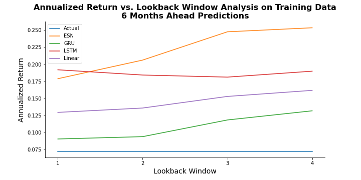
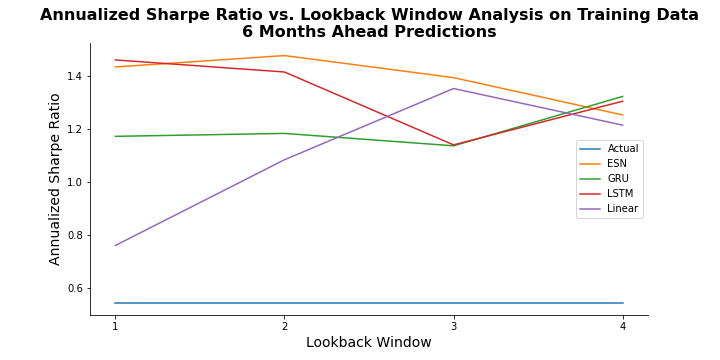
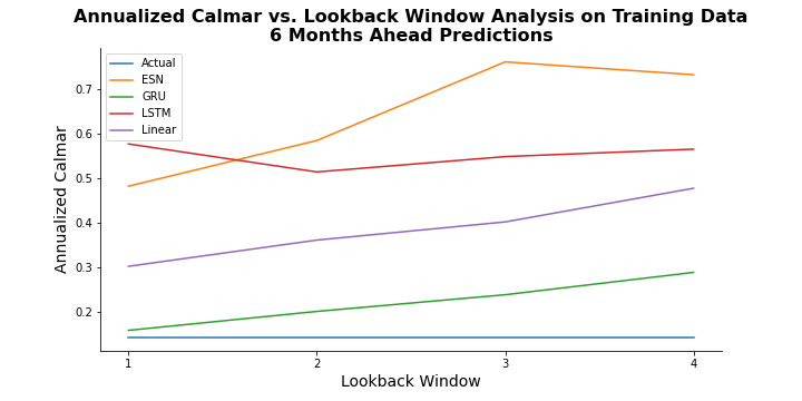
Figure 10: Comparison of Different Lookback Windows and Different Models for Six Months Ahead Prediction

Figure 10 indicates that ESN model performs the best in general for all metric during training period. The best annualized return is obtained for ESN with four years historical data. The annualized return tend to increase with an increase in lookback window for ESN, GRU, and ridge regression models. There is no clear pattern for annualized Sharpe ratio. The highest values are obtained for ESN with two years of historical data, and then LSTM with one year of historical data. Annualized Calmar ratio increases with longer historical data for GRU and ridge regression models, but the relationship is not linear for other models. The best annualized Calmar ratio is obtained for ESN with three years of historical data.

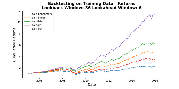
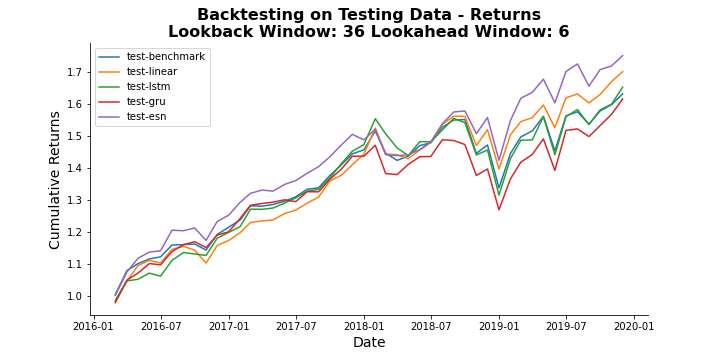
Figure 11: Backtesting Performance for Six Months Ahead Prediction Models (Three Years Lookback Window)

As seen in Figure 10, ESN is the superior model during training period for six month ahead predictions but different lookback windows obtain the highest values for each performance metric. In order to balance the performance, we pick ESN model with three years of historical data. Figure 11 shows the backtesting results for different models with three years of historical data. Consistent with near-term prediction results, all portfolios built by different models perform much better than the benchmark portfolio during training period, and the portfolio which is built based on ESN model obtains highest values. During testing period, ESN performs the best except the first half of 2018 where LSTM slightly outperforms. All models except GRU outperforms the benchmark portfolio within testing period. Appendix B.3 provides the performance metric plots during testing period, and the backtesting results for other lookback windows for six months ahead predictions.

Lookback Window	Model	In-Sample Performance			Out-of-Sample Performance
(Years)		Annualized Return	Sharpe Ratio	Calmar Ratio	Annualized Return	Sharpe Ratio	Calmar Ratio
Benchmark		7.40%	0.547	0.147	13.60%	1.200	0.990
1	Ridge	12.26%	1.136	0.288	12.54%	0.827	0.924
	LSTM	16.80%	1.386	0.498	16.46%	1.166	1.350
	GRU	12.78%	1.051	0.238	12.21%	0.830	0.869
	ESN	20.94%	1.530	0.617	15.35%	1.389	1.554
2	Ridge	13.95%	1.342	0.346	15.54%	0.956	1.351
	LSTM	21.18%	1.206	0.585	13.75%	1.378	1.100
	GRU	11.26%	1.173	0.215	13.45%	0.743	1.125
	ESN	20.81%	1.346	0.589	15.13%	1.391	1.397
3	Ridge	16.42%	1.289	0.444	14.00%	1.129	1.614
	LSTM	19.54%	1.159	0.566	12.11%	1.308	1.054
	GRU	13.42%	1.423	0.272	15.92%	0.878	1.440
	ESN	23.38%	1.091	0.679	12.50%	1.528	0.959
4	Ridge	17.00%	1.195	0.473	13.95%	1.186	1.133
	LSTM	20.62%	1.269	0.604	14.70%	1.372	1.111
	GRU	10.83%	1.186	0.218	14.94%	0.727	1.189
	ESN	25.08%	1.206	0.727	15.36%	1.569	1.207

Table 5: One Year Ahead Prediction Results - Performance Measures

Table 5 shows the performance of different models based on different amount of historical data for one year ahead predictions. In consistent to other prediction models, ESN and LSTM models outperform other models and benchmark portfolio in terms of annualized return and annualized Calmar ratio during training horizon. Despite the pattern is similar for annualized Sharpe ratio, GRU and ridge regression models also perform well for two years and three years of historical data. Testing period results indicate that ESN model is superior over other models if annualized Sharpe ratio is chosen as a performance metric. ESN model provides admissable annualized returns and annualized Calmar ratio, but the other models also outperform ESN model for different lookback windows.

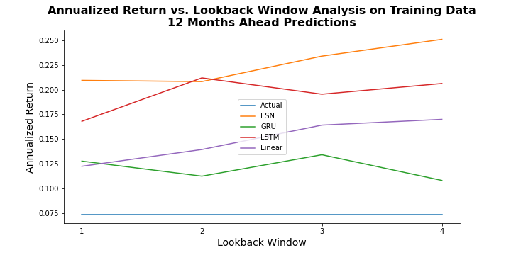
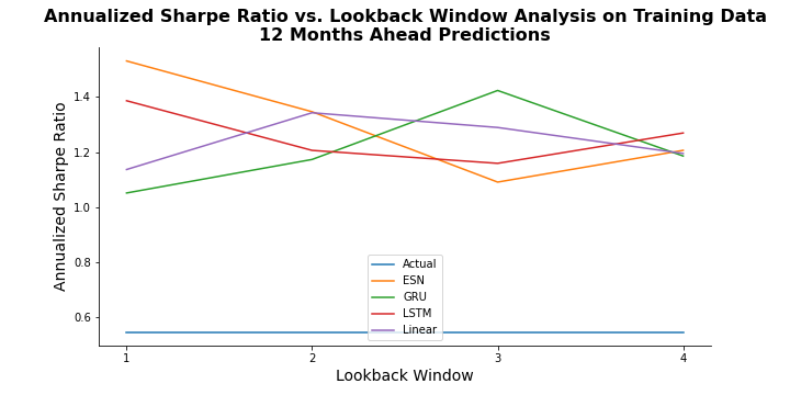
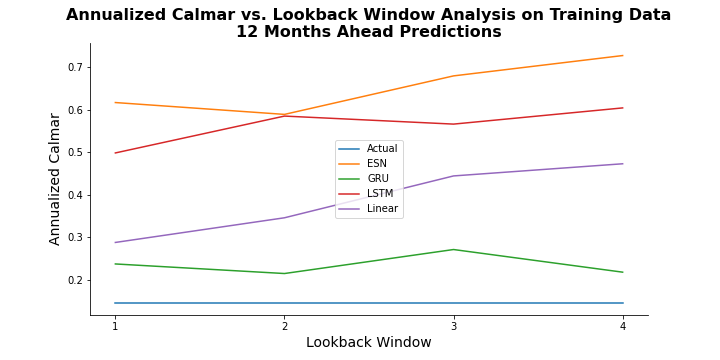
Figure 12: Comparison of Different Lookback Windows and Different Models for One Year Ahead Prediction

Figure 12 illustrates the relationship between different performance metrics and lookback window length for different models. Plots show that there is a positive relationship between annualized return and lookback window for ESN and ridge regression models during training period. Moreover, ESN achieves the best values for these performance metrics. Annualized Sharpe ratio decreases until three years of lookback window, and then it starts increasing for ESN and LSTM models. None of the models constantly outperforms the other models when annualized Sharpe ratio is the performance metric. The best value of annualized Sharpe ratio is attained with ESN model and one year of historical data.

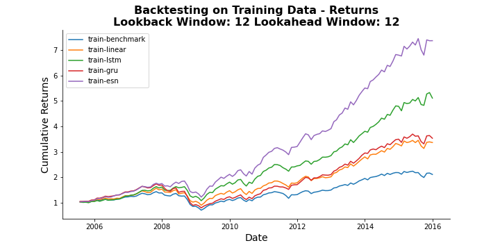
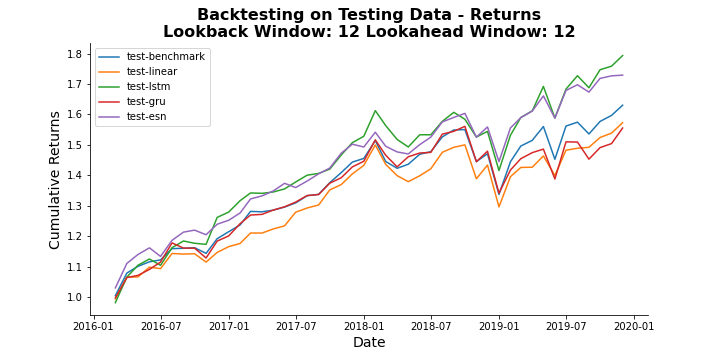
Figure 13: Backtesting Performance for One Year Ahead Prediction Models (One Year Lookback Window)

Figure 12 shows that ESN is superior to others when the performance metric is annualized return or annualized Calmar ratio, but there is no strong conclusion for annualized Sharpe ratio. Although the best values of annualized return and annualized Calmar ratio are both attained using ESN with four years of historical data, the value of annualized Sharpe ratio with the same setting is much lower than that of other models and other lookback windows. On the other hand, the best annualized Sharpe ratio is attained with ESN and one year of historical data. We select ESN with one year of historical data because the third best values for annualized return and annualized Calmar ratio are also obtained with ESN and one year lookback window. Figure 13 illustrates the backtesting results for all models which make use of one year of historical data. Training period results are in accordance with other prediction results. ESN model outperforms the other models, and all models perform better than equally weighted benchmark portfolio. ESN and LSTM models achieve similar cumulative returns over testing period, and they beat the performance of the benchmark portfolio significantly. Appendix B.4 includes the backtesting results for other lookback windows together with the performance metric plots for testing period for one year ahead sector ranking predictions.

6.4 Long-Term Results

Lastly, we observe the performance of our methodology in the long run by applying on two years ahead sector rankings prediction. We employ all models for different lookback windows ranging from one to five years.

Lookback Window	Model	In-Sample Performance			Out-of-Sample Performance
(Years)		Annualized Return	Sharpe Ratio	Calmar Ratio	Annualized Return	Sharpe Ratio	Calmar Ratio
Benchmark		5.36%	0.400	0.106	13.60%	1.200	0.990
1	Ridge	12.73%	1.042	0.334	12.22%	0.852	0.885
	LSTM	15.01%	1.219	0.369	12.43%	0.983	1.095
	GRU	12.11%	1.397	0.267	16.74%	0.789	1.484
	ESN	18.52%	1.211	0.529	14.52%	1.148	1.314
2	Ridge	15.14%	1.122	0.420	13.08%	1.010	1.137
	LSTM	18.56%	1.271	0.539	16.13%	1.150	1.053
	GRU	5.85%	1.079	0.110	13.20%	0.420	0.836
	ESN	20.51%	1.308	0.622	15.40%	1.277	1.084
3	Ridge	15.37%	1.402	0.428	15.73%	1.054	1.699
	LSTM	19.18%	1.369	0.552	13.93%	1.216	1.512
	GRU	8.49%	0.991	0.157	12.02%	0.578	0.852
	ESN	23.06%	1.119	0.681	13.24%	1.378	0.974
4	Ridge	16.60%	1.568	0.467	18.72%	1.101	2.159
	LSTM	17.64%	1.451	0.516	15.51%	1.142	1.417
	GRU	13.34%	1.067	0.331	13.06%	0.860	0.860
	ESN	24.04%	1.192	0.751	14.27%	1.432	1.028
5	Ridge	17.13%	1.179	0.472	14.02%	1.144	1.220
	LSTM	18.42%	1.448	0.533	17.44%	1.126	1.277
	GRU	7.06%	1.091	0.124	12.54%	0.493	0.964
	ESN	24.70%	1.185	0.786	15.16%	1.480	0.892

Table 6: Two Years Ahead Prediction Results - Performance Measures

Table 6 gives the overview of the performance of the models with different historical data span. During the training period, ESN achieves the highest annualized return and annualized Calmar ratio values. Despite ESN obtains desirable annualized Sharpe ratio values, other models may perform better than ESN for different lookback windows. In addition, ESN attains the highest annualized Sharpe ratios within testing period. During testing period, ESN performs moderate compared to other models for other metrics, but still outperforms the benchmark portfolio.

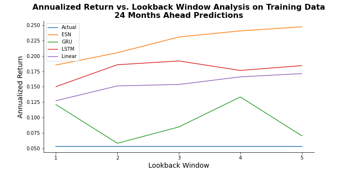
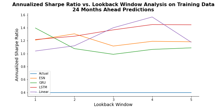
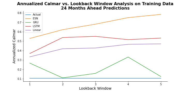
Figure 14: Comparison of Different Lookback Windows and Different Models for Two Years Ahead Prediction

Figure 14 shows that annualized return and annualized Calmar ratio follow similar patterns. The performance of ESN and ridge regression increases with an increase in the lookback window. ESN obtains highest values at each lookback window. The superiority of the models is not obvious from annualized Sharpe ratio plot. The plots indicate that ESN with five years of historical data attains the best annualized return and annualized Calmar ratio values. We select ESN with five years of historical data for illustrative purposes because it also obtains moderate annualized Sharpe ratio.

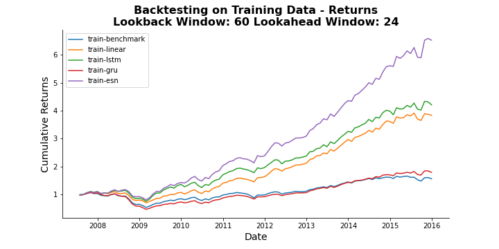
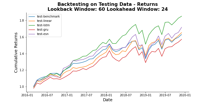
Figure 15: Backtesting Performance for Two Years Ahead Prediction Models (Five Years Lookback Window)

Figure 15 reveals the backtesting results of the models with the existence of five years historical data knowledge. Training period results are consistent with all other prediction horizon results. Although ESN outperforms the benchmark portfolio, LSTM performs better than ESN and other models. Appendix B.5 consists of the remaining backtesting results and performance metric plots over testing period for two years ahead predictions.

6.5 Diagnostics

In this section, we analyze the experimental results obtained by implementing the proposed methodology suggested in Section 5.

• Based on our experiments, we observe that our methodology is able to beat the performance of the benchmark portfolio no matter how long ahead we predict the sector rankings. Furthermore, our strategy for picking the models and lookback windows based on the balanced performance metrics always outperforms the benchmark portfolio for all prediction periods.

• The best performance is usually attained when the lookback window takes the largest value in the experiment range.

• Annualized return and annualized Calmar plots tend to follow the similar patterns for both training and testing horizons. The behavior of LSTM and ESN models are similar with the change of lookback window. GRU and ridge regression models also follow similar path according to lookback window. Although the relationship between the performance of other models and lookback windows is not clear, ESN model exhibits an increasing annualized return and annualized Calmar ratio as the lookback window increases.

• For each prediction period, all models achieve better cumulative returns than benchmark portfolio over training horizon. Moreover, the cumulative returns of all models are sorted in descending order as ESN, LSTM, ridge regression, GRU, and the benchmark portfolio. During testing period, ESN and LSTM models almost always outperform the benchmark portfolio. Although GRU and ridge regression models also provide admissible results, their relative performance according to benchmark is not stable enough.

• In comparison to LSTM and GRU, ESN model is easier to implement and faster. ESN model outperforms all other models and benchmark portfolio during training horizon, and the outstanding performance of ESN model also continues over testing horizon most of the time.

• In this paper, we chose a certain set of hyperparameters based on our preliminary experiments, but integrating hyperparameter tuning techniques such Bayesian optimization into our methodology may boost up the performance of the models and hence the overall methodology.

7 Conclusion and Future Work

In this paper, we develop a methodology for ranking sectors using a variety of common and sector-specific macroeconomic indicators. The methodology consists of two stages: prediction of sector index prices, and ranking sectors based on their predicted rate of returns. For each sector, we first apply RFE model to identify the most significant features, and then implement one of ridge regression, LSTM, GRU, and ESN models to predict the future sector index prices. We then rank the sectors based on their predicted rate of returns, and select top four ranked sectors for long-only strategy. We test the performance of our methodology over short-term, mid-term, and long-term. For each model, we also experiment with different lookback windows to show the robustness of the models based on the historical data used. Our numerical results show that the models generally performs better in the existence of longer lookback windows. We evaluate the performance of the models based on annualized return, annualized Sharpe ratio, and Calmar ratio. We pick the best performing model as the model satisfies admissible values for all performance measures. For each prediction horizon, ESN model is chosen based on this strategy. Our backtesting results indicate that our strategy that is built based on our methodology beats the performance of the benchmark portfolio consistently.

This paper consists of two consecutive stages where we first implement prediction models for each sector independently, and then rank the sectors based on their predicted returns. As a next step, we are going to develop a single step model that directly predicts the ranking of the sectors based on the market environment because employing prediction models separately for each sector increase the uncertainty of the overall performance. Our purpose is to implement learning-to-rank algorithms such as ListNet, BayesRank, and BoltzRank since they are specifically built for listwise ranking. We also plan to develop a methodology for obtaining sector-specific sentiment scores based on news articles, and integrate these sentiment scores into our current methodology as an input. Lastly, we build our methodology using public market information in this paper. For the future work, we aim at extending this methodology to private equity funds.

Appendices

Appendix A Macroeconomic Variables

Variables	Source	Frequency
GDP	https://fred.stlouisfed.org	Quarterly
Unemployment Rate	https://fred.stlouisfed.org	Monthly
CPI	https://fred.stlouisfed.org	Monthly
MORTGAGE30US	https://fred.stlouisfed.org	Weekly
Effective Federal Funds Rate	https://fred.stlouisfed.org	Monthly

Table A7: Macroeconomic Variables Common for All Sectors

Variables	Source	Frequency
Life Expectancy	https://www.macrotrends.net	Annual
Population	https://www.macrotrends.net	Annual
Birth Rate	https://www.macrotrends.net	Annual
Death Rate	https://www.macrotrends.net	Annual

Table A8: Macroeconomic Variables Considered for Healthcare Sector

Variables	Source	Frequency
U.S. Inflation Rate	https://www.macrotrends.net	Annual
5 Year Forward Inflation Rate	https://www.macrotrends.net	Annual
LIBOR Rate	https://www.macrotrends.net	Daily
TED Spread	https://www.macrotrends.net	Daily
Trade Balance % of GDP	https://www.macrotrends.net	Annual
Debt-to-GDP Ratio	https://www.macrotrends.net	Monthly

Table A9: Macroeconomic Variables Considered for Finance Sector

Variables	Source	Frequency
U.S. Inflation Rate	https://www.macrotrends.net	Annual
Gold	https://www.gold.org/goldhub/data/gold-prices	Monthly
Aluminum	https://www.indexmundi.com/commodities	Monthly
Copper	https://www.macrotrends.net	Daily
Hard Logs	https://www.indexmundi.com/commodities	Monthly
Lead	https://www.indexmundi.com/commodities	Monthly
Iron Ore	https://www.indexmundi.com/commodities	Monthly
Nickel	https://www.indexmundi.com/commodities	Monthly
Palladium	https://www.macrotrends.net	Daily
Platinum	https://www.macrotrends.net	Daily
Potassium Chloride	https://www.indexmundi.com/commodities	Monthly
Rock Phosphate	https://www.indexmundi.com/commodities	Monthly
Rubber	https://www.indexmundi.com/commodities	Monthly
Silver	https://www.indexmundi.com/commodities	Monthly
Tin	https://www.indexmundi.com/commodities	Monthly
Triple Superphosphate	https://www.indexmundi.com/commodities	Monthly
Urea	https://www.indexmundi.com/commodities	Monthly
Zinc	https://www.indexmundi.com/commodities	Monthly

Table A10: Macroeconomic Variables Considered for Materials Sector

Variables	Source	Frequency
Industrial Production Index	https://fred.stlouisfed.org	Monthly
Crude Oil Price	https://fred.stlouisfed.org	Monthly
Capacity Utilization	https://fred.stlouisfed.org	Monthly
Manufacturing	https://fred.stlouisfed.org	Monthly

Table A11: Macroeconomic Variables Considered for Industrials Sector

Variables	Source	Frequency
Consumer Confidence Index	https://data.oecd.org	Monthly
Business Confidence Index	https://data.oecd.org	Monthly

Table A12: Macroeconomic Variables Considered for Consumer Goods Sector

Variables	Source	Frequency
Import	https://fred.stlouisfed.org	Monthly
Export Value	https://data.oecd.org	Annual
Consumer Confidence Index	https://data.oecd.org	Monthly
R&D Value	https://data.oecd.org	Annual
Technology Investment	https://data.oecd.org	Annual

Table A13: Macroeconomic Variables Considered for Technology Sector

Variables	Source	Frequency
Crude Oil Price	https://fred.stlouisfed.org	Monthly
Refinery Utilization	https://www.eia.gov	Weekly
Primary Energy Production	https://www.eia.gov	Monthly
Primary Energy Consumption	https://www.eia.gov	Monthly
Import	https://fred.stlouisfed.org	Monthly

Table A14: Macroeconomic Variables Considered for Energy Sector

Variables	Source	Frequency
Crude Oil Price	https://fred.stlouisfed.org	Monthly
Refinery Utilization	https://www.eia.gov	Weekly
Import	https://fred.stlouisfed.org	Monthly
Natural Gas Consumption	https://www.eia.gov	Annual
Natural Gas Price	https://www.eia.gov	Annual
Interest Rate	https://fred.stlouisfed.org	Daily
Energy Consumption	https://www.eia.gov	Monthly
Electricity and Gas Production	https://www.eia.gov	Monthly

Table A15: Macroeconomic Variables Considered for Utilities Sector

Appendix B Performance Plots for Different Prediction Horizons

B.1 Next Month Prediction Performance Plots

Figure 16 illustrates how different models perform across different lookback windows during testing period. According to annualized Sharpe ratios, ESNs perform better than other models, and LSTM follows ESN. During the testing period, the annualized Sharpe ratio increases as more historical data is used for ESN model. There is no general pattern for annualized return and annualized Calmar ratio, but the best performing model for each lookback window is either LSTM or ESN.

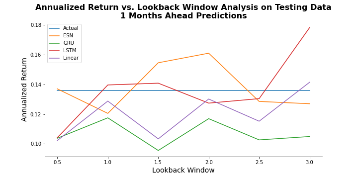
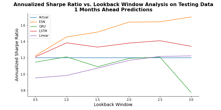
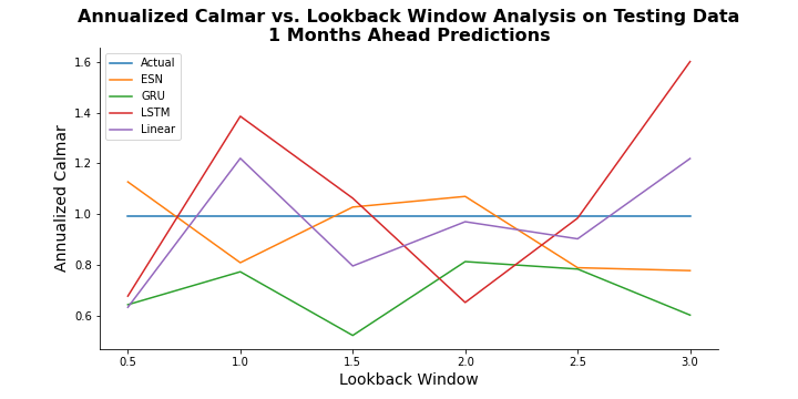
Figure 16: Comparison of Different Lookback Windows and Different Models for Next Month Prediction (Testing Period)

Figures 17, 18, 19, 20, and 21 illustrate the backtesting results for one month ahead ranking prediction with six months, one year, 1.5 years, 2.5 years, and three years, respectively. According to the plots, ESN constantly perform the best during the training period, and all four models are generating better returns than the benchmark portfolio. During the testing period, the results are not as obvious as the results obtained for training period. However, it can be observed that ESN and LSTM models performed better than GRU and Ridge regression models.

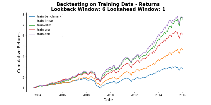
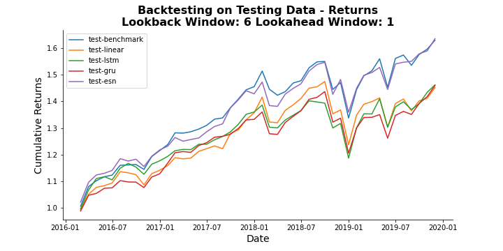
Figure 17: Backtesting Performance for Next Month Prediction Models (6 Months Lookback Window)

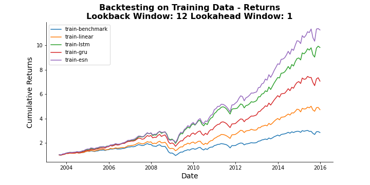
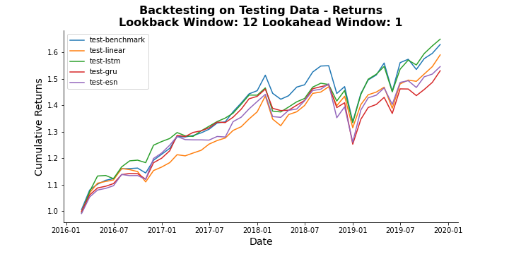
Figure 18: Backtesting Performance for Next Month Prediction Models (One Year Lookback Window)

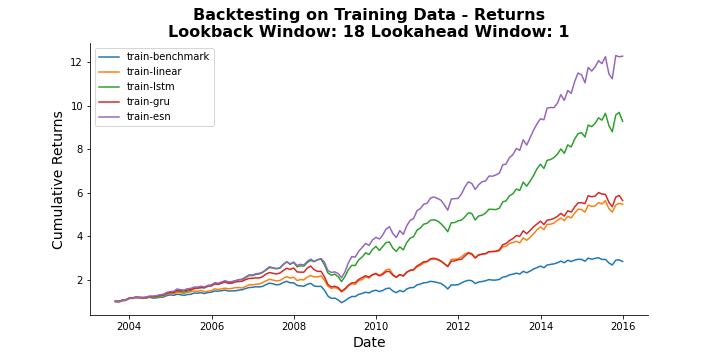
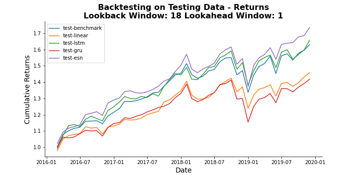
Figure 19: Backtesting Performance for Next Month Prediction Models (1.5 Years Lookback Window)

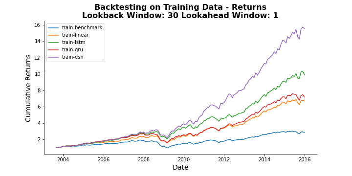
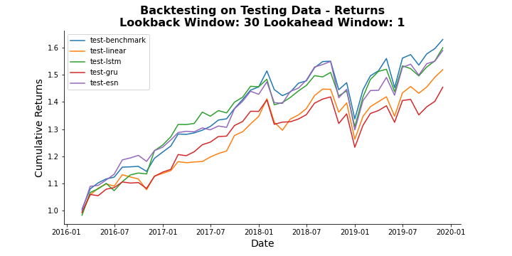
Figure 20: Backtesting Performance for Next Month Prediction Models (2.5 Years Lookback Window)

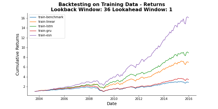
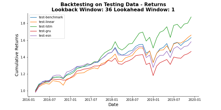
Figure 21: Backtesting Performance for Next Month Prediction Models (Three Years Lookback Window)

B.2 Three Months Ahead Prediction Performance Plots

Figure 22 illustrates how different models behave using different lookback windows during testing period for three months ahead predictions. There is no generic behavior obtained from all models, but ESN performs the best in terms of all performance metrics compared to other three models and also benchmark portfolio. Annualized return and annualized Sharpe ratio obtained from ESN models increase as the lookback window increases. For annualized Calmar ratio, the performance of all models increases until three years of historical data, but addition of one more year of data results in a decrease in the performance.

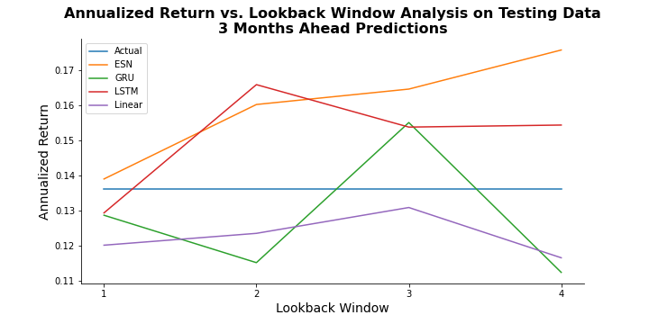
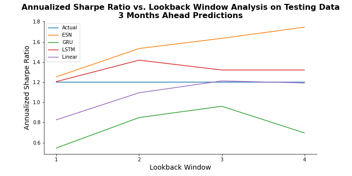
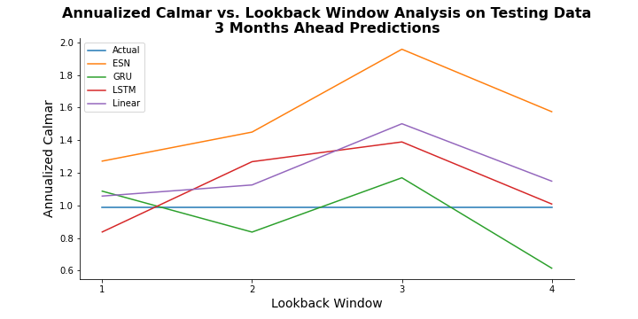
Figure 22: Comparison of Different Lookback Windows and Different Models for Three Months Ahead Prediction (Testing Period)

Figures 23, 24, and 25 provides the backtesting result for three months ahead predictions using one year, two years and three years of historical data, respectively. The results show that ESN outperforms all other models during training period, and LSTM follows ESN closely for one year and two years of historical data. Testing period plots show that ESN and LSTM models obtain higher cumulative returns than other models and benchmark portfolio most of the time. However, the difference between performance of different models is not as clear as the difference obtained during training horizon.

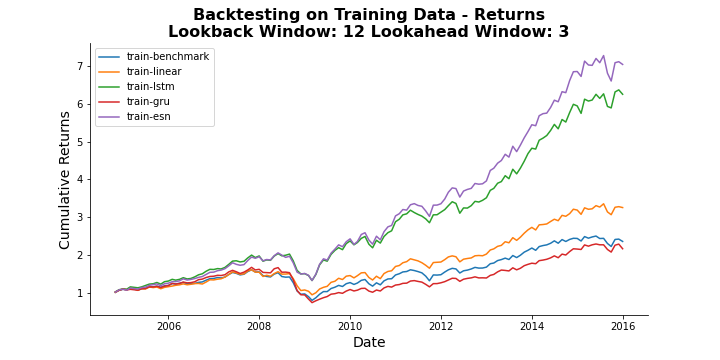
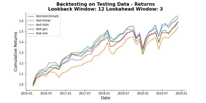
Figure 23: Backtesting Performance for Three Months Ahead Prediction Models (One Year Lookback Window)

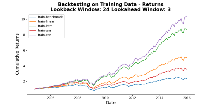
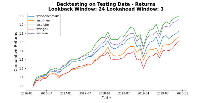
Figure 24: Backtesting Performance for Three Months Ahead Prediction Models (Two Years Lookback Window)

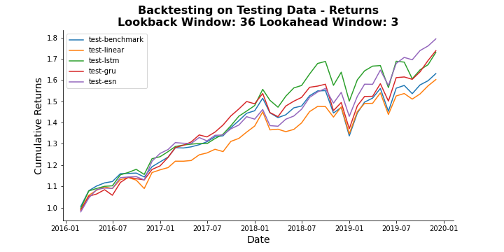
Figure 25: Backtesting Performance for Three Months Ahead Prediction Models (Three Years Lookback Window)

B.3 Six Months Ahead Prediction Performance Plots

Figure 26 illustrates the performance metrics plots for six months ahead prediction models during testing period. The plots show that ESN model generally performs the best for each performance metric and lookback window. Although annualized Sharpe ratio decreases after three years of historical data for ESN model, Sharpe ratio tends to increase as the lookback window increases for all models. For annualized returns and annualized Calmar ratio, ESN and ridge regression follow similar patterns. The same behavior is observed between LSTM and GRU models.

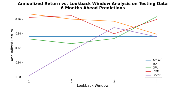
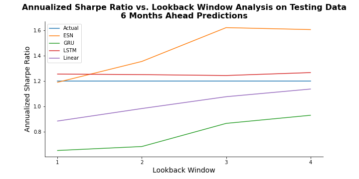
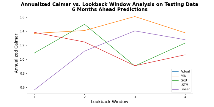
Figure 26: Comparison of Different Lookback Windows and Different Models for Six Months Ahead Prediction (Testing Period)

Figures 27, 28, and 29 illustrate the backtesting results for six months ahead prediction models. The results are consistent with near-term backtesting results. All models perform better than benchmark portfolio over training horizon, and ESN performs the best for each lookback window. Although ESN performs the best for one year and two years lookback windows during testing period, GRU outperforms all other models when four years of historical data is used. LSTM model perfoms the second best for all lookback windows within testing period.

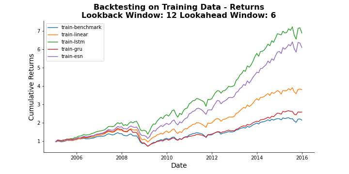
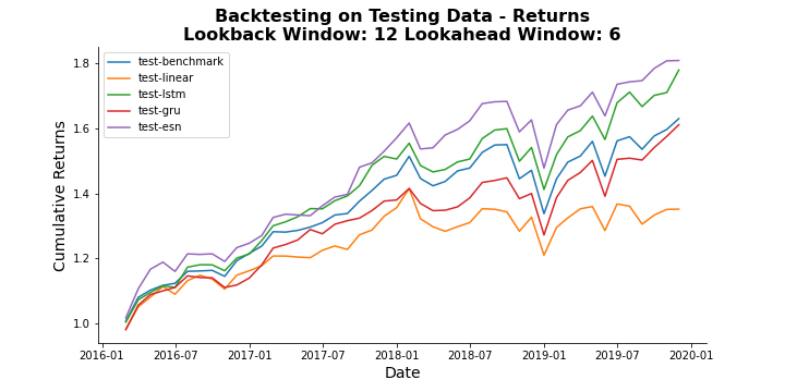
Figure 27: Backtesting Performance for Six Months Ahead Prediction Models (One Year Lookback Window)

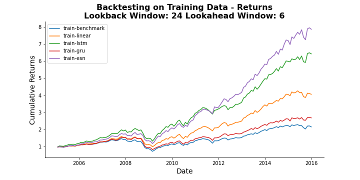
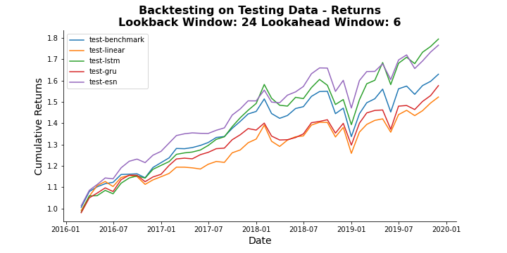
Figure 28: Backtesting Performance for Six Months Ahead Prediction Models (Two Years Lookback Window)

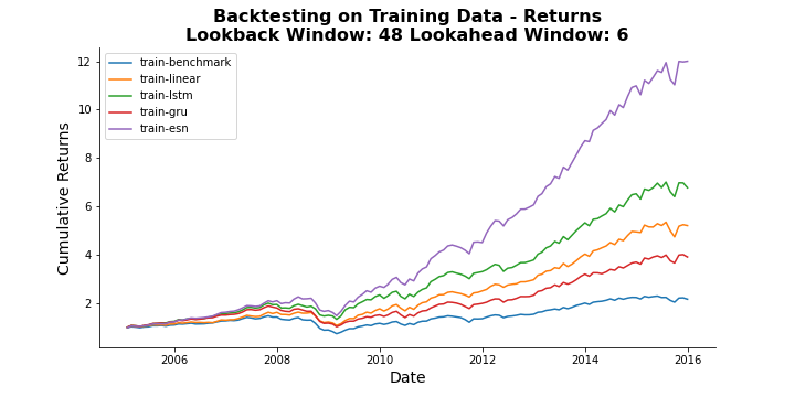
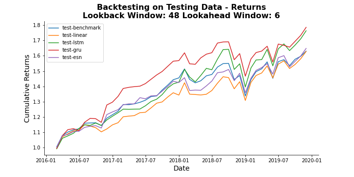
Figure 29: Backtesting Performance for Six Months Ahead Prediction Models (Four Years Lookback Window)

B.4 One Year Ahead Prediction Performance Plots

Figure 30 illustrates the performance of different models with different lookback windows over testing period for one year ahead sector ranking predictions. Both annualized return and annualized Calmar ratio plots reveal that the performance of ESN and LSTM models decrease until three years of historical data, and then it starts increasing. GRU and ridge regression models follow the similar patterns yet their behavior is opposite of ESN and LSTM. Annualized Sharpe ratio results indicate that ESN is superior to other models during testing period. Sharpe ratio values tend to increase for ESN and ridge regression models as lookback window increases.

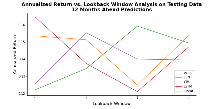
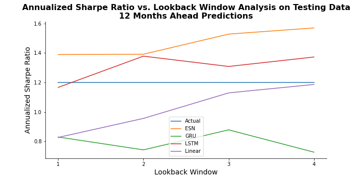
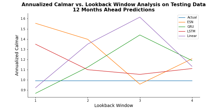
Figure 30: Comparison of Different Lookback Windows and Different Models for One Year Ahead Prediction (Testing Period)

Figures 31, 32, and 33 provides the backtesting results for one month ahead predictions with two years, three years, and four years of historical data, respectively. During the training period, all models perform better than benchmark portfolio, and ESN achieves highest cumulative returns when two years or three years of historical data is used. Although ESN generally performs better than benchmark portfolio, the results show that GRU model outperforms all other models when three or four years of historical data is used.

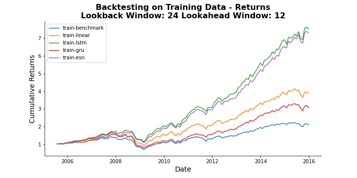
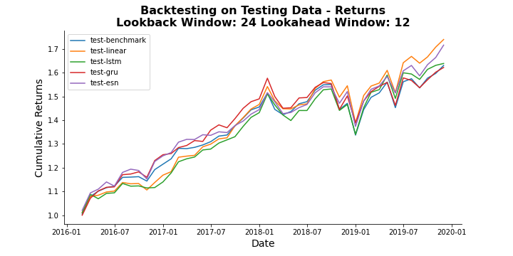
Figure 31: Backtesting Performance for One Year Ahead Prediction Models (Two Years Lookback Window)

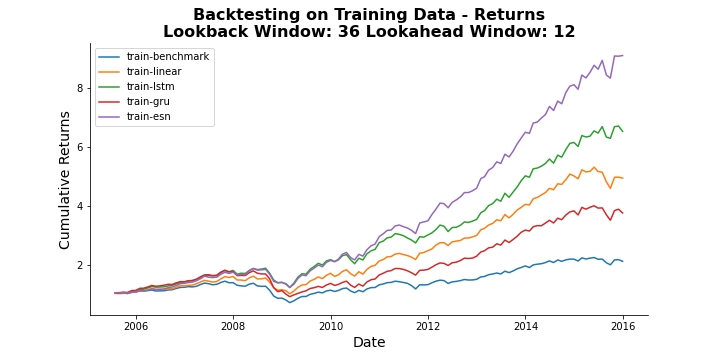
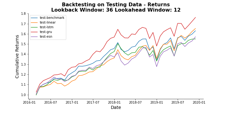
Figure 32: Backtesting Performance for One Year Ahead Prediction Models (Three Years Lookback Window)

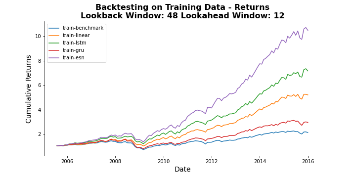
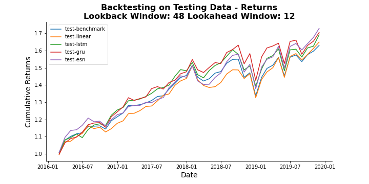
Figure 33: Backtesting Performance for One Year Ahead Prediction Models (Four Years Lookback Window)

B.5 Two Years Ahead Prediction Performance Plots

Figure 34 gives an overview of the performance of two years ahead prediction models. ESN outperforms other models in terms annualized Sharpe ratio, and the annualized Sharpe ratio has a positive relationship with length of the lookback window for ESN and ridge regression models. Annualized return and annualized Calmar ratio plots show that GRU performs the best when the lookback window is one year, but then ridge regression and LSTM obtains higher values in comparison to ESN and GRU.

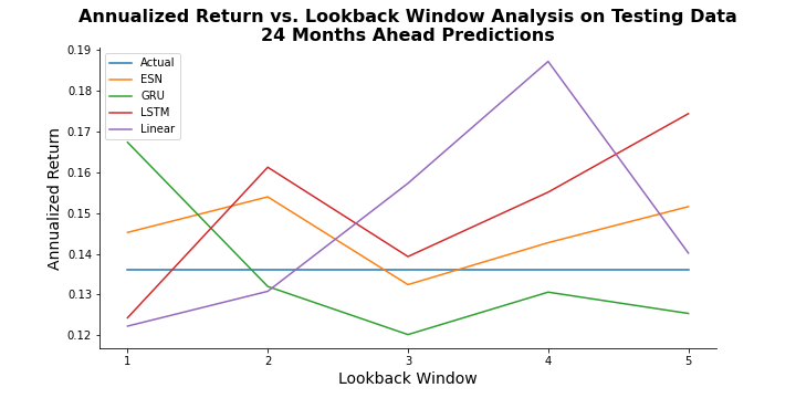
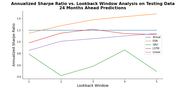
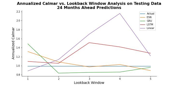
Figure 34: Comparison of Different Lookback Windows and Different Models for Two Years Ahead Prediction (Testing Period)

Figures 35, 36, 37, and 38 illustrate that ESN performs the best within training period. ESN still performs better than benchmark portfolio during testing period, but it is beaten by other models in the existence of different lookback windows.

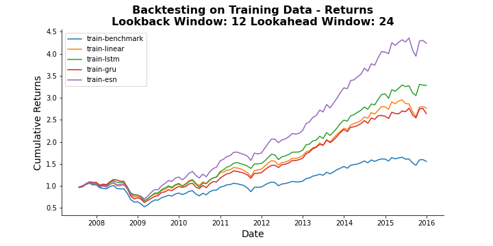
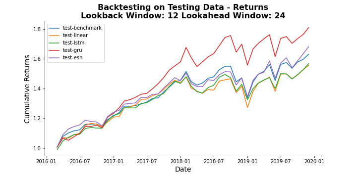
Figure 35: Backtesting Performance for Two Years Ahead Prediction Models (One Year Lookback Window)

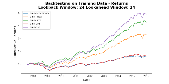
Figure 36: Backtesting Performance for Two Years Ahead Prediction Models (Two Years Years Lookback Window)

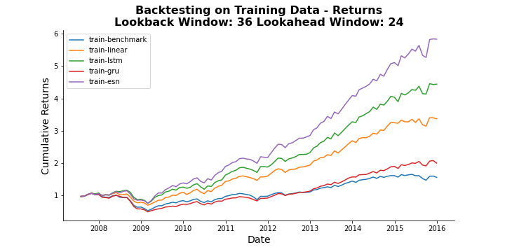
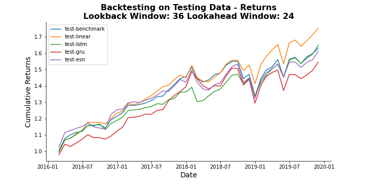
Figure 37: Backtesting Performance for Two Years Ahead Prediction Models (Third Years Lookback Window)

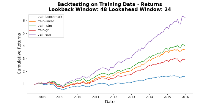
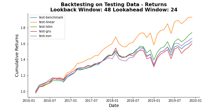
Figure 38: Backtesting Performance for Two Years Ahead Prediction Models (Four Years Lookback Window)

References

- [1] Anokye M Adam and George Tweneboah “Macroeconomic factors and stock market movement: Evidence from Ghana” In Available at SSRN 1289842, 2008
- [2] Nai-Fu Chen “Financial investment opportunities and the macroeconomy” In The Journal of Finance 46.2 Wiley Online Library, 1991, pp. 529–554
- [3] Nai-Fu Chen, Richard Roll and Stephen A Ross “Economic forces and the stock market” In Journal of business JSTOR, 1986, pp. 383–403
- [4] Kyunghyun Cho et al. “Learning phrase representations using RNN encoder-decoder for statistical machine translation” In arXiv preprint arXiv:1406.1078, 2014
- [5] James Chong, William P Jennings and G Michael Phillips “Eta® analysis of portfolios: The economy matters” In The Journal of Wealth Management 15.2 Institutional Investor Journals Umbrella, 2012, pp. 72–84
- [6] James Chong and G Michael Phillips “Sector rotation with macroeconomic factors” In The Journal of Wealth Management 18.1 Institutional Investor Journals Umbrella, 2015, pp. 54–68
- [7] James Chong and G Michael Phillips “Tactical Asset Allocation with Macroeconomic Factors” In The Journal of Wealth Management 17.1 Institutional Investor Journals Umbrella, 2014, pp. 58–69
- [8] Junyoung Chung, Caglar Gulcehre, KyungHyun Cho and Yoshua Bengio “Empirical evaluation of gated recurrent neural networks on sequence modeling” In arXiv preprint arXiv:1412.3555, 2014
- [9] Andrew D Clare and Stephen H Thomas “Macroeconomic Factors, the APT and the UK Stockmarket” In Journal of Business Finance & Accounting 21.3 Wiley Online Library, 1994, pp. 309–330
- [10] Mark J Flannery and Aris A Protopapadakis “Macroeconomic factors do influence aggregate stock returns” In The review of financial studies 15.3 Oxford University Press, 2002, pp. 751–782
- [11] Bo Gao and Ruo-En Ren “A New Sector Rotation Strategy and Its Performance Evaluation: Based on a Principal Component Regression Model” In Available at SSRN 2628058, 2015
- [12] Øystein Gjerde and Frode Saettem “Causal relations among stock returns and macroeconomic variables in a small, open economy” In Journal of International Financial Markets, Institutions and Money 9.1 Elsevier, 1999, pp. 61–74
- [13] Trevor Greetham and Michael Hartnett “The investment clock” In Journal of Women s Health, 2004
- [14] Isabelle Guyon, Jason Weston, Stephen Barnhill and Vladimir Vapnik “Gene selection for cancer classification using support vector machines” In Machine learning 46.1 Springer, 2002, pp. 389–422
- [15] Sepp Hochreiter and Jürgen Schmidhuber “Long short-term memory” In Neural computation 9.8 MIT Press, 1997, pp. 1735–1780
- [16] Arthur E Hoerl and Robert W Kennard “Ridge regression: applications to nonorthogonal problems” In Technometrics 12.1 Taylor & Francis Group, 1970, pp. 69–82
- [17] Arthur E Hoerl and Robert W Kennard “Ridge regression: Biased estimation for nonorthogonal problems” In Technometrics 12.1 Taylor & Francis Group, 1970, pp. 55–67
- [18] Mansor H Ibrahim and Hassanuddeen Aziz “Macroeconomic variables and the Malaysian equity market” In Journal of economic studies MCB UP Ltd, 2003
- [19] Herbert Jaeger “The “echo state” approach to analysing and training recurrent neural networks-with an erratum note” In Bonn, Germany: German National Research Center for Information Technology GMD Technical Report 148.34 Bonn, 2001, pp. 13
- [20] Herbert Jaeger, Mantas Lukoševičius, Dan Popovici and Udo Siewert “Optimization and applications of echo state networks with leaky-integrator neurons” In Neural networks 20.3 Elsevier, 2007, pp. 335–352
- [21] Francisco Jareño and Loredana Negrut “US stock market and macroeconomic factors” In Journal of Applied Business Research (JABR) 32.1, 2016, pp. 325–340
- [22] Chung S Kwon and Tai S Shin “Cointegration and causality between macroeconomic variables and stock market returns” In Global finance journal 10.1 Elsevier, 1999, pp. 71–81
- [23] Pooja Misra “An investigation of the macroeconomic factors affecting the Indian stock market” In Australasian Accounting, Business and Finance Journal 12.2, 2018, pp. 71–86
- [24] Tobias J Moskowitz and Mark Grinblatt “Do industries explain momentum?” In The Journal of finance 54.4 Wiley Online Library, 1999, pp. 1249–1290
- [25] Tarun K Mukherjee and Atsuyuki Naka “Dynamic relations between macroeconomic variables and the Japanese stock market: an application of a vector error correction model” In Journal of financial Research 18.2 Wiley Online Library, 1995, pp. 223–237
- [26] Thomas Raffinot and Sylvain Benoit “Investing through economic cycles with ensemble machine learning algorithms” In Available at SSRN 2785583, 2018
- [27] David E Rumelhart, Geoffrey E Hinton and Ronald J Williams “Learning representations by back-propagating errors” In nature 323.6088 Nature Publishing Group, 1986, pp. 533–536
- [28] Maximilian Sauer “Sector Rotation through the Business Cycle: A Machine Learning Regime Approach” In Available at SSRN 3473907, 2019
- [29] Tarika Singh, Seema Mehta and MS Varsha “Macroeconomic factors and stock returns: Evidence from Taiwan” In Journal of economics and international finance 3.4 Academic Journals, 2011, pp. 217–227
- [30] Xiaoya Wang, Yihui Zhang and YiXin Chen “A Novel Lasso Regression Model for Sector Rotation Trading Strategies with” Economy-Policy” Cycles” In 2020 IEEE International Conference on Big Data (Big Data), 2020, pp. 5473–5479 IEEE
- [31] Ye Zhu, Chao Yi and Yixin Chen “Utilizing Macroeconomic Factors for Sector Rotation based on Interpretable Machine Learning and Explainable AI”