Extended electron tails in electrostatic microinstabilities and the nonadiabatic response of passing electrons

Abstract

Ion-gyroradius-scale microinstabilities typically have a frequency comparable to the ion transit frequency. Due to the small electron-to-ion mass ratio and the large electron transit frequency, it is conventionally assumed that passing electrons respond adiabatically in ion-gyroradius-scale modes. However, in gyrokinetic simulations of ion-gyroradius-scale modes in axisymmetric toroidal magnetic fields, the nonadiabatic response of passing electrons can drive the mode, and generate fluctuations with narrow radial layers, which may have consequences for turbulent transport in a variety of circumstances. In flux tube simulations, in the ballooning representation, these instabilities reveal themselves as modes with extended tails. The small electron-to-ion mass ratio limit of linear gyrokinetics for electrostatic instabilities is presented, in axisymmetric toroidal magnetic geometry, including the nonadiabatic response of passing electrons and associated narrow radial layers. This theory reveals the existence of ion-gyroradius-scale modes driven solely by the nonadiabatic passing electron response, and recovers the usual ion-gyroradius-scale modes driven by the response of ions and trapped electrons, where the nonadiabatic response of passing electrons is small. The collisionless and collisional limits of the theory are considered, demonstrating parallels in structure and physical processes to neoclassical transport theory. By examining initial-value simulations of fastest-growing eigenmodes, the predictions for mass-ratio scaling are tested and verified numerically for a range of collision frequencies. Insights from the small electron-to-ion mass ratio theory may lead to a computationally efficient treatment of extended modes.

1 Introduction

The leading magnetic confinement fusion experiments achieve single particle confinement by exploiting strong magnetic fields that have nested toroidal flux surfaces: the Lorentz force prevents particles crossing the magnetic field in the perpendicular direction, but particles are free to stream along magnetic field lines. Despite this, there are still particle and heat losses from the confined plasma. Neoclassical transport is driven by interparticle Coulomb collisions in toroidal magnetic geometry, and turbulent transport is driven by the free energy available in the equilibrium temperature and density gradients.

Turbulence forms through the nonlinear saturation of microinstabilities. The most important microinstabilities for transport have frequencies $\omega$ comparable to the transit frequency of the constituent particle species, and perpendicular wavenumbers $k_{\perp}$ comparable to the inverse thermal gyroradius of the particles, i.e., $\omega\sim v_{\rm{th},s}/a\sim\rho_{\ast s}\Omega_{s}\ll\Omega_{s}$, and $k_{\perp}\rho_{\rm{th},s}\sim 1$, where $v_{\rm{th},s}=\sqrt{2T_{s}/m_{s}}$ is the thermal speed of the component species $s$, $a$ is a typical equilibrium length scale, $\Omega_{s}=Z_{s}eB/m_{s}c$ is the cyclotron frequency of the component species $s$, and $\rho_{\ast s}=\rho_{\rm{th},s}/a\ll 1$, with $\rho_{\rm{th},s}=v_{\rm{th},s}/\Omega_{s}$ the thermal gyroradius of the species $s$. In the above definitions, $T_{s}$ is the species temperature, $m_{s}$ is the species mass, $Z_{s}$ is the species charge number, $e$ is the proton charge, $B$ is the magnetic field strength, and $c$ is the speed of light. These microinstabilities are extended along magnetic field lines, with parallel wave numbers such that $k_{\|}qR\sim 1$, where $qR$ is the connection length, $q\sim 1$ is the safety factor and $R\sim a$ is the major radius. A diffusive random walk estimate for the heat flux $Q_{\rm s}$ driven by instabilities at the scale $\rho_{\rm{th},s}$ gives $Q_{\rm s}\sim Q_{\rm gb,s}=\rho_{\ast s}^{2}n_{s}T_{s}v_{\rm{th},s}$, with $n_{s}$ the equilibrium plasma density of species $s$. To obtain this estimate, we use that the macroscopic profiles have a scale of order $a$, and that turbulent eddies transport heat by a step length $\rho_{\rm{th},s}$ in a timescale $v_{\rm{th},s}/a$.

A plasma has multiple particle species: the simplest plasma consists of ions, with charge $Z_{\rm{i}}e$ and mass $m_{{\rm{i}}}$, and electrons, with charge $-e$ and mass $m_{{\rm{e}}}$. In a fusion plasma with deuterium ions, the separation between the ion and electron masses has significant consequences for the nature of the turbulence and the underlying instabilities. Since $\sqrt{m_{{\rm{i}}}/m_{{\rm{e}}}}\approx 60$, we have that $\rho_{\rm{th,i}}\gg\rho_{\rm{th,e}}$ and $v_{\rm{th,i}}\ll v_{\rm{th,e}}$, i.e., instabilities can be driven over a wide range of space and time scales. Historically, research has largely focused on transport and instabilities driven at the larger scale of the ion gyroradius. This is for the simple reason that the heat flux estimate $Q_{\rm gb,i}$ for $\rho_{\rm{th,i}}$-scale turbulence dominates the heat flux estimate $Q_{\rm gb,e}$ for $\rho_{\rm{th,e}}$-scale turbulence by $\left({m_{\rm{i}}}/{m_{\rm{e}}}\right)^{1/2}\gg 1$. However, it is important not to discount the $\rho_{\rm{th,e}}$ scales for several reasons. It is known that $\rho_{\rm{th,e}}$-scale turbulence can drive experimentally relevant heat fluxes that exceed the $Q_{\rm gb,e}$ estimate by a large order-unity factor [1, 2, 3, 4]. Recently, expensive direct numerical simulations (DNS) with realistic electron-to-hydrogen-ion-mass ratio [5, 6] and realistic electron-to-deuterium-ion-mass ratio [7, 8, 9, 10, 6, 11] have demonstrated the existence and significance of cross-scale interactions between turbulence at the scales of $\rho_{\rm{th,i}}$ and $\rho_{\rm{th,e}}$. Finally, as we will demonstrate in this paper, even familiar long-wavelength modes with binormal wave numbers $k_{y}\rho_{\rm{th,i}}\sim 1$ may have narrow radial structures near mode-rational surfaces that satisfy $k_{r}\rho_{\rm{th,e}}\sim 1$, with $k_{r}$ the radial wave number. These structures result from the dynamics of passing electrons [12, 13], and may be important for understanding cross-scale interactions in multiscale DNS, cf. [6]. We will see that there are novel $k_{y}\rho_{\rm{th,i}}\sim 1$ modes driven by the electron response to the electron temperature gradient (ETG) in the $k_{r}\rho_{\rm{th,e}}\sim 1$ narrow layer, and we will see that even the familiar ion temperature gradient (ITG) mode can exhibit $k_{r}\rho_{\rm{th,e}}\sim 1$ features.

Anisotropy between the radial wave number $k_{r}$ and the binormal wave number $k_{y}$ arises naturally in linear modes in toroidal magnetic fields because of the presence of magnetic shear $\hat{s}$. In the presence of magnetic shear, linear modes are conveniently described in terms of “ballooning” modes that follow the magnetic field line many times around the torus [14]. Ballooning modes have wave fronts that rotate with position along the magnetic field line. As we shall describe with more precision later, in a ballooning mode the radial wave number $k_{r}$ satisfies $k_{r}\propto-k_{y}\hat{s}\theta$ for large $\theta$, where $\theta$ is the extended poloidal angle that is used to describe the position along the field line as it winds around the torus. Therefore, it is possible for $k_{y}\rho_{\rm{th,i}}\sim 1$ modes to have extended “ballooning tails” at $\theta\gg 1$ that correspond to $k_{r}\rho_{\rm{th,i}}\gg 1$ components. In the real-space picture, modes with extended ballooning tails are modes with significant amplitude in a layer around mode-rational flux surfaces – flux surfaces where the field line winds onto itself after an integer number of toroidal and poloidal turns. With this in mind, we can understand the origin of electron-driven ballooning tails with a simple physical argument. On irrational flux surfaces, where a single field line covers the flux surface, rapidly moving passing electrons can sample the entire flux surface and respond adiabatically. However, on mode-rational flux surfaces, passing electrons can only sample a subset of the flux surface and hence have a nonadiabatic response.

Linear modes with extended ballooning tails have been observed in simulations with a variety of equilibrium conditions, for example, in simulations of electrostatic modes in core tokamak conditions [12, 13] and in the pedestal [15], as well as in electromagnetic simulations of linear micro-tearing modes in spherical and conventional tokamaks [16, 17, 18]. Although simulations of linear modes are inexpensive compared to nonlinear simulations of turbulence, simulations of modes with extended ballooning tails can be remarkably costly. In implicit codes, the computational expense arises from the need to resolve variation of geometric quantities on the scales of $2\pi$ in ballooning angle, combined with the need to simulate very large ballooning angles with scales $\theta\gg 2\pi$: this leads to an expensive matrix problem. In explicit codes, in addition to the size of the problem in $\theta$, small time steps are required to resolve kinetic electron physics in modes with frequencies comparable to the ion transit frequency. The results presented in this paper are intended as a step towards efficient reduced models of extended electron-driven modes.

In this paper we obtain an asymptotic theory, valid in the limit of $\left(m_{\rm{e}}/m_{\rm{i}}\right)^{1/2}\rightarrow 0$, for electrostatic modes that exist at the long wavelengths of the ion gyroradius scale, i.e., $k_{y}\rho_{\rm{th,i}}\sim 1$. Reduced models of these modes must provide a reduced treatment of the electron response. In the simplest case, for example, the classical ITG mode calculation [19, 20], the electron response is taken to be adiabatic. More advanced calculations retain the bounce-averaged response due to trapped electrons, needed to capture trapped-electron modes (TEMs), see, e.g., [21, 22]. The nonadiabatic response of passing electrons is traditionally neglected, despite evidence from DNS that indicates that the nonadiabatic passing electron response can play a significant role in electrostatic modes: pioneering work showed that the passing electron response can alter transport in linear modes and fully nonlinear turbulence [12]. This observation has subsequently been reinforced by a variety of investigations, see, for example [13, 6, 23, 24, 25, 26, 27]. In this paper, we will show that, in the $\left(m_{\rm{e}}/m_{\rm{i}}\right)^{1/2}\rightarrow 0$ limit, there are in fact two classes of modes existing at $k_{y}\rho_{\rm{th,i}}\sim 1$: first, the familiar ion or trapped-electron response-driven modes (e.g., the ITG mode or the TEM) that rely on a potential localised at $\theta\sim 1$; and second, ETG modes that are driven by the passing electron response in the large $\theta$ tail of the ballooning mode. We find the large $\theta$ equations that govern the electron response in the tail of the ballooning mode, and we provide the matching conditions necessary to connect them to the $\theta\sim 1$ region. We use simulations performed with the gyrokinetic code GS2 [28] to show that the orderings used to derive these equations are satisfied by numerical examples of both classes of mode.

The clearest physical ordering for the novel passing-electron-response-driven modes is $k_{y}\rho_{\rm{th,e}}\sim qR\omega/v_{\rm{th,e}}\ll 1$, i.e., they are ETG modes at long wavelengths, that feature a radial layer with $k_{r}\rho_{\rm{th,e}}\sim 1$, with an asymptotic separation between the transit frequency $v_{\rm{th,e}}/qR$ and the frequency of the drive $\omega_{\ast}\sim\omega$. We can treat the familiar ITG modes and TEMs in the same formalism as the novel passing-electron-driven modes by simply making the maximal ordering $k_{y}\rho_{\rm{th,e}}\sim\left(m_{\rm{e}}/m_{\rm{i}}\right)^{1/2}\ll 1$. Mathematically, the two classes of mode are distinguished in the formalism by the matching condition for the passing electrons at $\theta\sim 1$. This is true in both the “collisionless” limit

$$\frac{v_{\rm{th,e}}}{qR}\gg\omega\sim\omega_{\ast}\sim\nu_{\rm{ee}}\sim\nu_{\rm{ei}},$$ (1)

where $\nu_{\rm{ee}}$ and $\nu_{\rm{ei}}$ are the electron self-collision and the electron-ion collision frequencies, respectively, and in the “collisional” limit where

$$\frac{v_{\rm{th,e}}}{qR}\sim\nu_{\rm{ee}}\sim\nu_{\rm{ei}}\gg\omega\sim\omega_{\ast}.$$ (2)

The remainder of this paper is structured as follows. In section 2, we briefly review the electrostatic gyrokinetic model that is the starting point for this work. Those familiar with gyrokinetics may skip to section 3, where we identify a convenient form of the gyrokinetic equation that we use to describe electron dynamics. We obtain the asymptotic theory of collisionless modes in section 4, and we obtain the asymptotic theory of collisional modes in section 5. We compare the results of sections 4 and 5 to numerical simulations in section 6. Finally, in section 7, we discuss the implications of these results and possible extensions of the theory. Included in this paper are appendices with results pertaining to the plasma response at large $\theta$. First, in A, we give a detailed analysis of the ion nonadiabatic response at large $\theta$. In B we obtain the equations governing the electron response in the collisional limit. In C, we solve the Spitzer problem necessary to obtain the neoclassical parallel and perpendicular flux contributions to the electron mode equations. In D, we obtain the classical perpendicular flux contributions to the electron mode equations. In E, we obtain the parallel and perpendicular fluxes for the electron mode equations in the highly collisional (Pfirsh-Schlüter) limit. In F, we obtain the parallel and perpendicular fluxes for the electron mode equations in the banana regime of collisionality in a small inverse aspect ratio device. Finally, in G we obtain the electron matching conditions in the collisional limit.

2 Electrostatic gyrokinetic equations

In this section, we briefly review the linear, electrostatic, $\delta\!f$ gyrokinetic model [29] that is the starting point for the analysis in this paper. In gyrokinetic theory, the microinstability mode frequency $\omega$ is taken to be much smaller than the cyclotron frequency $\Omega_{s}$ at which particles gyrate around the magnetic field direction $\bm{b}=\bm{B}/B$, where $\bm{B}$ is the magnetic field. The mode frequency $\omega$ is taken to be of order the transit frequency $v_{\rm{th},s}/a$. The spatial scale of the fluctuations perpendicular to the magnetic field line is of order the thermal gyroradius $\rho_{\rm{th},s}=v_{\rm{th},s}/\Omega_{s}$, and the fundamental gyrokinetic expansion parameter is $\rho_{\ast s}=\rho_{\rm{th},s}/a$. In $\delta\!f$ gyrokinetics, the fluctuating distribution function $\delta\!f_{s}$ for each species $s$ is a sum of the nonadiabatic response $h_{s}$, and the adiabatic response $-Z_{s}e\phi F_{0s}/T_{s}$, i.e.,

$$\delta\!f_{s}({\bm{r}},\bm{v},t)=h_{s}({\bm{R}},\varepsilon,\lambda,t)-\frac{Z_{s}e\phi({\bm{r}},t)}{T_{s}}F_{0s},$$ (3)

where $\phi$ is the fluctuating electrostatic potential, $F_{0s}$ is the equilibrium Maxwellian distribution, ${\bm{r}}$ is the particle position, $\bm{v}$ is the particle velocity, and we have indicated that $h_{s}$ is a function of guiding centre position ${\bm{R}}={\bm{r}}-\bm{\rho}_{s}$ (with $\bm{\rho}_{s}=\bm{b}\times\bm{v}/\Omega_{s}$), energy $\varepsilon=m_{s}v^{2}/2$ (with $v=|\bm{v}|$), and pitch angle $\lambda=v_{\perp}^{2}/v^{2}B$ (with $v_{\perp}=|\bm{v}-\bm{b}\bm{b}\cdot\bm{v}|$), whereas $\phi$ is a function of ${\bm{r}}$ but not of $\bm{v}$. In this paper we consider linear theory, and so we make the eikonal ansatz $h_{s}({\bm{R}},t)=\sum_{\bm{k}_{\perp}}h_{s,\bm{k}_{\perp}}\exp{\left[{\rm{i}}(\bm{k}_{\perp}\cdot{\bm{R}}-\omega t)\right]}$, and $\phi({\bm{r}},t)=\sum_{\bm{k}_{\perp}}\phi_{\bm{k}_{\perp}}\exp{\left[{\rm{i}}(\bm{k}_{\perp}\cdot{\bm{r}}-\omega t)\right]}$, where $\bm{k}_{\perp}$ is the perpendicular-to-the-field wave vector. Henceforth, we drop the $\bm{k}_{\perp}$ subscripts on the Fourier coefficients.

2.1 The gyrokinetic equation and quasineutrality

The linear, electrostatic gyrokinetic equation is

$$v_{\|}\bm{b}\!\cdot\!\nabla\theta\frac{\partial h_{s}{}}{\partial\theta}+{\rm{i}}(\bm{k}_{\perp}\cdot\bm{v}_{{\rm{M}},{s}}-\omega)h_{s}{}-C^{\rm{GK}}_{s}[h_{s}{}]={\rm{i}}\left(\omega_{\ast,s}-\omega\right)J_{0s}F_{0s}\frac{Z_{s}e\phi{}}{T_{s}},$$ (4)

where $v_{\|}=\bm{b}\cdot\bm{v}$, $\theta$ is the poloidal angle coordinate that measures distance along the magnetic field line, $\bm{v}_{{\rm{M}},{s}}=(\bm{b}/\Omega_{s})\times\left(v_{\|}^{2}\bm{b}\cdot\nabla\bm{b}+v_{\perp}^{2}\nabla B/2B\right)$ is the magnetic drift, and the finite Larmor radius effects are modelled by the 0^th Bessel function of the first kind $J_{0s}=J_{0}(b_{s})$, with $b_{s}=k_{\perp}v_{\perp}/\Omega_{s}$, and $k_{\perp}=|\bm{k}_{\perp}|$. Note that $\Omega_{\rm{i}}=Z_{\rm{i}}eB/m_{{\rm{i}}}c>0$, whereas $\Omega_{\rm{e}}=-eB/m_{{\rm{e}}}c<0$. The frequency $\omega_{\ast,s}$ contains the equilibrium drives of instability: $\omega_{\ast,s}/\omega^{n}_{\ast,s}=1+\eta_{s}\left(\varepsilon/T_{s}-3/2\right)$, with $\omega^{n}_{\ast,s}=-(ck_{\alpha}T_{s}/Z_{s}e)d\ln n_{s}/d\psi$, and $n_{s}$ the equilibrium number density of species $s$, $\alpha$ the dimensionless binormal coordinate, $k_{\alpha}$ the binormal wavenumber with respect to $\alpha$, $\psi$ the poloidal magnetic flux ($\alpha$ and $\psi$ are defined in section 2.2), and $\eta_{s}=d\ln T_{s}/d\ln n_{s}$. Finally, the collision operator $C^{\rm{GK}}_{s}[\cdot]$ is shorthand for the linearised gyrokinetic collision operator of the species $s$.

For ions, the linearised gyrokinetic collision operator is defined by

$$C^{\rm{GK}}_{\rm{i}}\left[h_{{\rm{i}}}\right]=\left\langle{\exp{\left[{\rm{i}}\bm{k}_{\perp}\!\cdot\!\bm{\rho}_{i}\right]}C_{\rm{ii}}\left[\exp{\left[-{\rm{i}}\bm{k}_{\perp}\!\cdot\!\bm{\rho}_{i}\right]}h_{{\rm{i}}}\right]}\right\rangle^{\gamma},$$ (5)

with $C_{\rm{ii}}[\cdot]$ the linearised self-collision operator of the ion species, and $\left\langle{\cdot}\right\rangle^{\gamma}$ the gyrophase average at fixed $\varepsilon$ and $\lambda$. The self-collision operator of the species $s$, $C_{ss}[\cdot]$, is defined by

$$C_{ss}\left[f\right]=\frac{2\pi Z_{s}^{4}e^{4}\ln\Lambda}{m_{s}^{2}}\frac{\partial}{\partial\bm{v}}\cdot\int F_{0s}F_{0s}^{\prime}\bm{U}(\bm{v}-\bm{v}^{\prime})\cdot\left(\frac{\partial}{\partial\bm{v}}\left(\frac{f}{F_{0s}}\right)-\frac{\partial}{\partial\bm{v}^{\prime}}\left(\frac{f^{\prime}}{F_{0s}^{\prime}}\right)\right)\;d^{3}\bm{v}^{\prime},$$ (6)

where $f$ is a distribution function, and we have used the shorthand notation $f=f(\bm{v})$, $f^{\prime}=f(\bm{v}^{\prime})$, $F_{0s}=F_{0s}(\bm{v})$, $F_{0s}^{\prime}=F_{0s}(\bm{v}^{\prime})$, and

$$\bm{U}(\bm{v}-\bm{v}^{\prime})=\frac{\bm{I}|\bm{v}-\bm{v}^{\prime}|^{2}-(\bm{v}-\bm{v}^{\prime})(\bm{v}-\bm{v}^{\prime})}{|\bm{v}-\bm{v}^{\prime}|^{3}},$$ (7)

with $\bm{I}$ the identity matrix. We note that the Coloumb logarithm $\ln\Lambda\approx 17$ [30]. We define the ion self-collision frequency $\nu_{\rm{ii}}=4\sqrt{\pi}Z_{\rm{i}}^{4}n_{\rm{i}}e^{4}\ln\Lambda/3m_{{\rm{i}}}^{1/2}T_{\rm{i}}^{3/2}$ and the electron self-collision frequency $\nu_{\rm{ee}}=4\sqrt{2\pi}n_{\rm{e}}e^{4}\ln\Lambda/3m_{{\rm{e}}}^{1/2}T_{\rm{e}}^{3/2}$ following Braginskii [31], noting the factor of $\sqrt{2}$ difference in the definitions of $\nu_{\rm{ee}}$ and $\nu_{\rm{ii}}$.

For electrons, the linearised gyrokinetic collision operator is defined by

$$C^{\rm{GK}}_{\rm{e}}\left[h_{{\rm{e}}}\right]=\left\langle{\exp{\left[{\rm{i}}\bm{k}_{\perp}\!\cdot\!\bm{\rho}_{e}\right]}C_{\rm{ee}}\left[\exp{\left[-{\rm{i}}\bm{k}_{\perp}\!\cdot\!\bm{\rho}_{e}\right]}h_{{\rm{e}}}\right]}\right\rangle^{\gamma}$$

$$+\left\langle{\exp{\left[{\rm{i}}\bm{k}_{\perp}\!\cdot\!\bm{\rho}_{e}\right]}\mathcal{L}\left[\exp{\left[-{\rm{i}}\bm{k}_{\perp}\!\cdot\!\bm{\rho}_{e}\right]}h_{{\rm{e}}}-\frac{m_{{\rm{e}}}\bm{v}\cdot\delta\!\bm{u}_{\rm{i}}}{T_{\rm{e}}}F_{0e}\right]}\right\rangle^{\gamma},$$ (8)

where $C_{\rm{ee}}[\cdot]$ is the linearised self-collision operator of the electron species, defined by equation (6), and

$${\mathcal{L}\left[f\right]=\frac{3\sqrt{\pi}}{8}\nu_{\rm{ei}}v_{\rm{th,e}}^{3}\frac{\partial}{\partial\bm{v}}\cdot\left(\frac{v^{2}\bm{I}-\bm{v}\bm{v}}{v^{3}}\cdot\frac{\partial f}{\partial\bm{v}}\right),}$$ (9)

is the Lorentz collision operator resulting from electron-ion collisions, with the electron-ion collision frequency $\nu_{\rm{ei}}=4\sqrt{2\pi}Z_{\rm{i}}^{2}n_{\rm{i}}e^{4}\ln\Lambda/3m_{{\rm{e}}}^{1/2}T_{\rm{e}}^{3/2}$ defined following Braginskii [31]. In equation (8),

$$\delta\!\bm{u}_{\rm{i}}=\frac{1}{n_{\rm{i}}}\int\left(J_{0{\rm{i}}}v_{\|}\bm{b}+{\rm{i}}J_{1{\rm{i}}}\frac{v_{\perp}}{k_{\perp}}\bm{k}_{\perp}\times\bm{b}\right)\;h_{{\rm{i}}}\;d^{3}\bm{v},$$ (10)

where $J_{1s}=J_{1}(b_{s})$ is the 1^st Bessel function of the first kind.

For a simple two-species plasma of ions and electrons, quasineutrality implies that the equilibrium densities satisfy $Z_{\rm{i}}n_{\rm{i}}=n_{\rm{e}}$. In the electrostatic limit, the system of gyrokinetic equations for the fluctuations is closed by the quasineutrality relation. The quasineutrality relation has the form

$$\left(\frac{Z_{\rm{i}}T_{\rm{e}}}{T_{\rm{i}}}+1\right)\frac{e\phi{}}{T_{\rm{e}}}=\frac{\delta\!n_{\rm{i}}}{n_{\rm{i}}}-\frac{\delta\!n_{\rm{e}}}{n_{\rm{e}}},$$ (11)

where the fluctuating nonadiabatic densities $\delta\!n_{s}$ are defined by

$$\delta\!n_{s}=\int J_{0s}h_{s}{}\;d^{3}\bm{v}.$$ (12)

2.2 Magnetic coordinates and boundary conditions

To describe the plane perpendicular to the magnetic field line, we use the dimensionless binormal field-line-label coordinate $\alpha$, and the flux label $\psi$, defined such that the magnetic field may be written in the Clebsch form

$$\bm{B}=\nabla\alpha\times\nabla\psi.$$ (13)

We restrict our attention to axisymmetric magnetic fields of the form

$$\bm{B}=I\nabla\zeta+\nabla\zeta\times\nabla\psi,$$ (14)

where $\zeta$ is the toroidal angle, and $I(\psi)$ is the toroidal current function. An explicit formula for $\alpha$, in terms of $\psi$, $\zeta$, and the poloidal angle $\theta$, may be obtained by equating expressions (13) and (14):

$$\alpha(\psi,\zeta,\theta)=\zeta-q(\psi)\theta-\nu(\psi,\theta),$$ (15)

with the safety factor

$$q(\psi)=\frac{1}{2\pi}\int^{2\pi}_{0}\frac{\bm{B}\cdot\nabla\zeta}{\bm{B}\cdot\nabla\theta^{\prime}}d\theta^{\prime},$$ (16)

and

$$\nu(\psi,\theta)=\int^{\theta}_{0}\frac{\bm{B}\cdot\nabla\zeta}{\bm{B}\cdot\nabla\theta^{\prime}}d\theta^{\prime}-q\theta.$$ (17)

Note that $\nu(\psi,2\pi)=\nu(\psi,0)=0$. Using the $(\psi,\alpha)$ coordinates, we write the perpendicular wave vector as

$$\bm{k}_{\perp}=k_{\psi}\nabla\psi+k_{\alpha}\nabla\alpha,$$ (18)

with the field-aligned radial and binormal wave numbers $k_{\psi}$ and $k_{\alpha}$, respectively.

In the study of linear modes, it is convenient to consider the coordinate $\theta$ as an extended ballooning angle, and to replace $k_{\psi}$ with $\theta_{0}=k_{\psi}/q^{\prime}k_{\alpha}$, where $q^{\prime}=dq/d\psi$. In this formulation, $h_{\theta_{0},k_{\alpha}}=h_{\theta_{0},k_{\alpha}}(\theta)$, with $-\infty<\theta<\infty$ and the boundary conditions

$$h_{\theta_{0},k_{\alpha}}(\theta)=0{\rm{~{}at~{}}}\theta\rightarrow-\infty,{\rm{~{}for~{}}}v_{\|}>0,{\rm~{}and}$$

$$h_{\theta_{0},k_{\alpha}}(\theta)=0{\rm{~{}at~{}}}\theta\rightarrow\infty,{\rm{~{}for~{}}}v_{\|}<0.$$ (19)

Much of the discussion in the following sections of this paper is focused on the behaviour of the solution at large $\theta$. The large $\theta$ part of the mode corresponds to a narrow radial layer in the real-space representation. To see this, consider the (contravariant) radial wave number

$$k_{r}=\bm{k}_{\perp}\cdot\nabla r=(\theta_{0}-\theta)k_{\alpha}\frac{dq}{dr}|\nabla r|^{2}-k_{\alpha}(q\nabla\theta\cdot\nabla r+\nabla\nu\cdot\nabla r),$$ (20)

where $r=r(\psi)$ is a minor radial coordinate that is a function of $\psi$ only, and has dimensions of length. For large $|\theta_{0}-\theta|$, we find that $k_{r}\simeq(\theta_{0}-\theta)k_{\alpha}(dq/dr)|\nabla r|^{2}$, i.e., we may obtain narrow radial structures in a ballooning mode by either imposing a large $\theta_{0}=k_{\psi}/q^{\prime}k_{\alpha}$, or by following the field line, as a result of magnetic shear.

It will be interesting to consider the behaviour of the magnetic drift. The term due to the magnetic drift, ${\rm{i}}\bm{k}_{\perp}\cdot\bm{v}_{{\rm{M}},{s}}$, may be written in the following convenient form

$${\rm{i}}\bm{k}_{\perp}\cdot\bm{v}_{{\rm{M}},{s}}={\rm{i}}k_{\alpha}\bm{v}_{{\rm{M}},{s}}\cdot(\nabla\alpha+\theta\nabla q)+{\rm{i}}k_{\alpha}\frac{dq}{dr}(\theta_{0}-\theta)\bm{v}_{{\rm{M}},{s}}\cdot\nabla r.$$ (21)

We note that the quantity $\nabla\alpha+\theta\nabla q=\nabla\zeta-q\nabla\theta-\nabla\nu$ contains no secular variation in $\theta$. Hence, for large $|\theta_{0}-\theta|$ the magnetic drift is dominated by the radial component: ${\rm{i}}\bm{k}_{\perp}\cdot\bm{v}_{{\rm{M}},{s}}\simeq{\rm{i}}k_{r}\bm{v}_{{\rm{M}},{s}}\cdot\nabla r/|\nabla r|^{2}$ for $|\theta_{0}-\theta|\gg 1$. Thus, the leading behaviour of a ballooning mode at large $\theta$ should be expected to involve the radial magnetic drift. We will often make use of the identity for the radial magnetic drift in an axisymmetric magnetic field,

$$\bm{v}_{{\rm{M}},{s}}\cdot\nabla\psi=v_{\|}\bm{b}\!\cdot\!\nabla\theta\frac{\partial}{\partial\theta}\left(\frac{Iv_{\|}}{\Omega_{s}}\right).$$ (22)

Finally, we complete this discussion of coordinates by defining a field-aligned radial wave number and binormal wave number with dimensions of length, $k_{x}$ and $k_{y}$, respectively. First, we define local radial and binormal coordinates with units of length, $x=(\psi-\psi_{0})(d\psi/dx)^{-1}$ and $y=(\alpha-\alpha_{0})(d\alpha/dy)^{-1}$, respectively, where $(\psi_{0},\alpha_{0})$ are the coordinates of the field line of interest. Then, the field-aligned radial wavenumber $k_{x}=k_{\psi}(d\psi/dx)$ and the binormal wave number $k_{y}=k_{\alpha}(d\alpha/dy)$. We take the proportionality constants to be $d\psi/dx=rI/qR_{0}$ and $d\alpha/dy=(I/R_{0})dr/d\psi$. The functions $I(\psi)$, $r(\psi)$, and $q(\psi)$ appearing in the proportionality constants should be evaluated on the local flux surface of interest, and $R_{0}=(R_{\rm max}+R_{\rm min})/2$ is a reference major radius, with $R_{\rm max}$ and $R_{\rm min}$ the maximum and minimum major radial positions on the flux surface, respectively. Note that for circular concentric flux surfaces $R_{0}$ is the major radius at the magnetic axis. Using these normalisations, we find that the true radial wave number $k_{r}\simeq(\theta_{0}-\theta)k_{y}\hat{s}\hat{\kappa}|\nabla r|^{2}$ for $|\theta_{0}-\theta|\gg 1$, with the magnetic shear defined by $\hat{s}=(r/q)dq/dr$ and the geometrical factor $\hat{\kappa}=(qR_{0}/Ir)d\psi/dr$.

3 A convenient form of the gyrokinetic equation

It is possible to use the identity for the radial magnetic drift in equation (22) to rewrite the gyrokinetic equation in a novel way that simplifies the asymptotic analysis of the electron response. Collecting terms due to parallel streaming and radial drifts, we find that we can write

$$v_{\|}\bm{b}\!\cdot\!\nabla\theta\frac{\partial h_{s}}{\partial\theta}+{\rm{i}}k_{\alpha}q^{\prime}(\theta_{0}-\theta)v_{\|}\bm{b}\!\cdot\!\nabla\theta\frac{\partial}{\partial\theta}\left(\frac{Iv_{\|}}{\Omega_{s}}\right)h_{s}$$

$$\qquad\qquad=\exp{\left[-{\rm{i}}\lambda_{s}(\theta_{0}-\theta)\right]}v_{\|}\bm{b}\!\cdot\!\nabla\theta\frac{\partial}{\partial\theta}\left(\exp{\left[{\rm{i}}\lambda_{s}(\theta_{0}-\theta)\right]}h_{s}\right)+{\rm{i}}\lambda_{s}v_{\|}\bm{b}\!\cdot\!\nabla\theta\;h_{s},$$ (23)

with

$$\lambda_{s}=\frac{k_{\alpha}q^{\prime}Iv_{\|}}{\Omega_{s}}.$$ (24)

Note that $\lambda_{s}$ should not be confused with the pitch angle coordinate $\lambda$. We define the new function $H_{s}$ by

$$H_{s}=\exp{\left[{\rm{i}}\lambda_{s}(\theta_{0}-\theta)\right]}h_{s},$$ (25)

and hence we can rewrite the gyrokinetic equation, equation, (4), as

$$v_{\|}\bm{b}\!\cdot\!\nabla\theta\frac{\partial H_{s}}{\partial\theta}+{\rm{i}}(\omega_{{\rm{M}},s}-\omega)H_{s}-\widehat{C}_{s}[H_{s}]={\rm{i}}\left(\omega_{\ast,s}-\omega\right)\exp{\left[{\rm{i}}\lambda_{s}(\theta_{0}-\theta)\right]}J_{0s}F_{0s}\frac{Z_{s}e\phi{}}{T_{s}},$$ (26)

where

$$\omega_{{\rm{M}},s}=k_{\alpha}\left(\bm{v}_{{\rm{M}},{s}}\cdot\left(\nabla\alpha+\theta\nabla q\right)+\bm{b}\!\cdot\!\nabla\theta\frac{q^{\prime}Iv_{\|}^{2}}{\Omega_{s}}\right),$$ (27)

and

$$\widehat{C}_{s}[H_{s}]=\exp{\left[{\rm{i}}\lambda_{s}(\theta_{0}-\theta)\right]}C^{\rm{GK}}_{s}[\exp{\left[-{\rm{i}}\lambda_{s}(\theta_{0}-\theta)\right]}H_{s}{}].$$ (28)

It is also useful to consider the form of the nonadiabatic density appearing in the quasineutrality relation, equation (11). In terms of $H_{s}$, we can write the nonadiabatic, fluctuating density $\delta\!n_{s}$ as

$$\delta\!n_{s}=\int\exp{\left[-{\rm{i}}\lambda_{s}(\theta_{0}-\theta)\right]}J_{0s}H_{s}{}\;d^{3}\bm{v}.$$ (29)

When the gyrokinetic equation is written in terms of $H_{s}$, the oscillation in the distribution function due to the radial magnetic drift appears explicitly as the phase $\exp{\left[{\rm{i}}\lambda_{s}(\theta_{0}-\theta)\right]}$ – this phase may be thought of in analogy to the phase $\exp{\left[{\rm{i}}\bm{k}_{\perp}\cdot\bm{\rho}_{s}\right]}$ arising from the finite Larmor radius in gyrokinetic theory. In fact, the appearance of $\exp{\left[{\rm{i}}\lambda_{s}(\theta_{0}-\theta)\right]}$ is due to the finite particle drift orbit width. This may be noted by writing $\lambda_{s}(\theta_{0}-\theta)=k_{\alpha}q^{\prime}(\theta_{0}-\theta)\Delta\psi$, recalling that $\Delta\psi=Iv_{\|}/\Omega_{s}$ is the excursion in flux label $\psi$ made by trapped particles in a banana orbit [32], and finally, noting that, in the limit of large $|\theta_{0}-\theta|$, $\lambda_{s}(\theta_{0}-\theta)\simeq k_{r}(dr/d\psi)\Delta\psi/|\nabla r|^{2}$.

4 Long-wavelength collisionless electrostatic modes in the $\left(m_{\rm{e}}/m_{\rm{i}}\right)^{1/2}\rightarrow 0$ limit

In this section, we derive reduced model equations for long-wavelength, electrostatic modes in the $\left(m_{\rm{e}}/m_{\rm{i}}\right)^{1/2}\rightarrow 0$ limit, using the “collisionless” ordering (1), with $k_{y}\rho_{\rm{th,i}}\sim\theta_{0}\sim 1$. In this ordering, the extent of the ballooning mode is controlled by a balance of free streaming, precessional drifts, finite-Larmor-radius and finite-orbit-width phases, and the orbit-averaged electron collision operator, with the result that the mode extends to a ballooning angle $\theta\sim(k_{y}\hat{s}\rho_{\rm{th,e}})^{-1}\sim\left({m_{\rm{i}}}/{m_{\rm{e}}}\right)^{1/2}\gg 1$. For consistency with the electron species, we take the ion self-collision frequency $\nu_{\rm{ii}}\sim\left(m_{\rm{e}}/m_{\rm{i}}\right)^{1/2}v_{\rm{th,i}}/qR\ll v_{\rm{th,i}}/qR\sim\omega$.

We first examine the $\theta\sim 1$ region of the ballooning mode. This discussion reveals the existence of passing-electron-response-driven modes, in addition to the usual ion-response-driven and trapped-electron-response-driven modes, and motivates an examination of the $\theta\sim\left({m_{\rm{i}}}/{m_{\rm{e}}}\right)^{1/2}$ region of the collisionless ballooning mode in section 4.2. To aid comprehension, we summarise the results for trapped-electron-response-driven and ion-response-driven modes in section 4.3, and for passing-electron-response-driven modes in section 4.4. Finally, in section 4.5, we comment on the relationship between the derivation of gyrokinetics and the derivation of the reduced model equations for the electron response: although these theories have fundamental differences, they have a similar structure, relying on the finite Lamor radius and the finite magnetic drift orbit width of particles, respectively.

4.1 Outer solution – $k_{r}\rho_{\rm{th,i}}\sim 1$

We define the outer region of the mode to be the region where $k_{r}\rho_{\rm{th,i}}\sim\theta\sim 1$. In real space, the outer region is the large-scale region far from the rational flux surface. In the collisionless ordering, it is natural to expand the electrostatic potential $\phi$, distribution functions $h_{s}$, and frequency $\omega$ in $\left(m_{\rm{e}}/m_{\rm{i}}\right)^{1/2}$: for the potential $\phi$, we expand

$$\phi{}=\phi^{(0)}+\phi^{(1)}+\Or\left(\left(\frac{m_{\rm{e}}}{m_{\rm{i}}}\right)\phi\right),$$ (30)

with $\phi^{(n)}\sim\left(m_{\rm{e}}/m_{\rm{i}}\right)^{n/2}\phi^{(0)}$. We make expansions of the same form as (30) for $h_{s}$ and $\omega$, with $h_{s}{}^{(n)}\sim\left(m_{\rm{e}}/m_{\rm{i}}\right)^{n/2}(e\phi{}/T_{\rm{e}})F_{0s}$ and $\omega^{(n)}\sim\left(m_{\rm{e}}/m_{\rm{i}}\right)^{n/2}\omega$.

4.1.1 Ion response in the outer region.

For the ion species, we start with the usual form of the gyrokinetic equation, equation (4). In the collisionless limit, the leading order equation for the ion response is

$$v_{\|}\bm{b}\!\cdot\!\nabla\theta\frac{\partial h_{{\rm{i}}}{}^{(0)}{}}{\partial\theta}+{\rm{i}}\left(\bm{k}_{\perp}\cdot\bm{v}_{\rm{M,i}}-\omega^{(0)}\right)h_{{\rm{i}}}{}^{(0)}{}={\rm{i}}\left(\omega_{\ast,{\rm{i}}}-\omega^{(0)}\right)J_{0{\rm{i}}}F_{0i}\frac{Z_{\rm{i}}e\phi^{(0)}}{T_{\rm{i}}}.$$ (31)

Using equation (31), and the estimates $\omega\sim v_{\rm{th,i}}/a\sim\omega_{\ast,{\rm{i}}}$ and $b_{{\rm{i}}}\sim 1$, we find that $h_{{\rm{i}}}{}^{(0)}/F_{0i}\sim e\phi^{(0)}/T_{\rm{i}}$. The equation for the nonadiabatic ion density is

$$\frac{\delta\!n^{(0)}_{\rm{i}}}{n_{\rm{i}}}=\int J_{0{\rm{i}}}\frac{h_{{\rm{i}}}{}^{(0)}}{n_{\rm{i}}}\;d^{3}\bm{v}\sim\frac{e\phi^{(0)}}{T_{\rm{e}}},$$ (32)

where we have assumed that $T_{\rm{i}}\sim T_{\rm{e}}$ in the final estimate of equation (32). As expected, the ion nonadiabatic response contributes at leading order to $\phi{}$ in the outer region.

4.1.2 Electron response in the outer region.

For the electron species, we use the modified form of the gyrokinetic equation, equation (26). We do this to avoid integrating the radial magnetic drift $\bm{v}_{\rm{M,e}}\cdot\nabla\psi$ by parts in $\theta$ at every order when applying transit or bounce averages. The leading order equation for the electron response is

$$v_{\|}\bm{b}\!\cdot\!\nabla\theta\frac{\partial H^{(0)}_{{\rm{e}}}{}}{\partial\theta}=0,$$ (33)

where we have used that the electron parallel streaming term is larger than every other term in equation (26) by the ordering (1). We note that for electrons $\lambda_{{\rm{e}}}\sim\left(m_{\rm{e}}/m_{\rm{i}}\right)^{1/2}$, and hence, for $\theta_{0}\sim\theta\sim 1$ the phase $\exp{\left[{\rm{i}}\lambda_{{\rm{e}}}(\theta_{0}-\theta)\right]}$ may be expanded as

$$\exp{\left[{\rm{i}}\lambda_{{\rm{e}}}(\theta_{0}-\theta)\right]}=1+{\rm{i}}\lambda_{{\rm{e}}}(\theta_{0}-\theta)-\frac{\lambda_{{\rm{e}}}^{2}}{2}(\theta_{0}-\theta)^{2}+\Or\left(\left(\frac{m_{\rm{e}}}{m_{\rm{i}}}\right)^{3/2}\right).$$ (34)

As a consequence of equation (33), the leading-order nonadiabatic electron response is independent of $\theta$ for $\theta\sim 1$. The remainder of the expansion must be carried out separately for passing and trapped particles.

Trapped particles occupy the range of pitch angles $1/B_{\rm max}<\lambda\leq 1/B(\theta)$, with $B_{\rm max}$ the maximum value of $B(\theta)$. In each well, trapped particles bounce at the upper and lower bounce points, $\theta^{+}_{b}$ and $\theta^{-}_{b}$, respectively. Equation (33) for trapped particles states that $H^{(0)}_{{\rm{e}}}$ is constant in $\theta$ within each magnetic well. Imposing the trapped particle boundary conditions

$$h_{{\rm{e}}}(\theta^{\pm}_{b},\sigma=1)=h_{{\rm{e}}}(\theta^{\pm}_{b},\sigma=-1),$$ (35)

where $\sigma=v_{\|}/|v_{\|}|$, and using equation (25), we find that $H^{(0)}_{{\rm{e}}}(\sigma=1)=H^{(0)}_{{\rm{e}}}(\sigma=-1)$, and so $H^{(0)}_{{\rm{e}}}$ is independent of $(\theta,\sigma)$. The trapped electron piece of the distribution function $H^{(0)}_{{\rm{e}}}$ is determined by the equation for the next order in the electron response

$$v_{\|}\bm{b}\!\cdot\!\nabla\theta\frac{\partial H^{(1)}_{{\rm{e}}}}{\partial\theta}+{\rm{i}}(\omega_{\rm{M,e}}-\omega^{(0)})H^{(0)}_{{\rm{e}}}-\mathcal{C}[H^{(0)}_{{\rm{e}}}]=-{\rm{i}}\left(\omega_{\ast,{\rm{e}}}-\omega^{(0)}\right)F_{0e}\frac{e\phi^{(0)}{}}{T_{\rm{e}}},$$ (36)

where we have used that for $b_{{\rm{e}}}=\Or(\left(m_{\rm{e}}/m_{\rm{i}}\right)^{1/2})$, $J_{0{\rm{e}}}=1+\Or(m_{{\rm{e}}}/m_{{\rm{i}}})$, and $\exp{\left[{\rm{i}}\lambda_{{\rm{e}}}(\theta_{0}-\theta)\right]}=1+\Or\left(\left(m_{\rm{e}}/m_{\rm{i}}\right)^{1/2}\right)$, and we have employed $\bm{k}_{\perp}\cdot\bm{\rho}_{e}\sim b_{{\rm{e}}}\sim\left(m_{\rm{e}}/m_{\rm{i}}\right)^{1/2}$ to reduce the collision operator in equation (36) to the drift-kinetic electron collision operator

$$\mathcal{C}\left[\cdot\right]=C_{\rm{ee}}\left[\cdot\right]+\mathcal{L}\left[\cdot\right].$$ (37)

To close equation (36), we introduce the bounce average for trapped particles

$$\left\langle{\cdot}\right\rangle^{\rm{b}}=\frac{\sum_{\sigma}\int^{\theta^{+}_{b}}_{\theta^{-}_{b}}d\theta\;(\cdot)/|v_{\|}|\bm{b}\!\cdot\!\nabla\theta}{2\int^{\theta^{+}_{b}}_{\theta^{-}_{b}}d\theta/|v_{\|}|\bm{b}\!\cdot\!\nabla\theta}.$$ (38)

Applying $\left\langle{\cdot}\right\rangle^{\rm{b}}$ to equation (36), we find the solvability condition

$${\rm{i}}\left(\left\langle{\omega_{\rm{M,e}}}\right\rangle^{\rm{b}}-\omega^{(0)}\right)H^{(0)}_{{\rm{e}}}-\left\langle{\mathcal{C}[H^{(0)}_{{\rm{e}}}]}\right\rangle^{\rm{b}}=-{\rm{i}}\left(\omega_{\ast,{\rm{e}}}-\omega^{(0)}\right)F_{0e}\frac{e\left\langle{\phi^{(0)}}\right\rangle^{\rm{b}}}{T_{\rm{e}}},$$ (39)

where we have used the property

$$\left\langle{v_{\|}\bm{b}\!\cdot\!\nabla\theta\frac{\partial f}{\partial\theta}}\right\rangle^{\rm{b}}=0$$ (40)

of the bounce average, valid for any $f=f_{\theta_{0},k_{\alpha}}(\varepsilon,\lambda,\sigma,\theta)$ satisfying the bounce condition $f_{\theta_{0},k_{\alpha}}(\varepsilon,\lambda,\sigma=1,\theta^{\pm}_{b})=f_{\theta_{0},k_{\alpha}}(\varepsilon,\lambda,\sigma=-1,\theta^{\pm}_{b})$.

Passing particles occupy the range of pitch angles $0\leq\lambda\leq 1/B_{\rm max}$, and hence, passing particles are free to travel between magnetic wells. For passing electrons, equation (33) determines that, for a given $(\theta_{0},k_{\alpha})$ mode, $H^{(0)}_{{\rm{e}}}$ is a constant in $\theta$ for each sign of the parallel velocity $\sigma$, i.e., $H^{(0)}_{{\rm{e}}}=H^{(0)}_{{\rm{e}}}(\varepsilon,\lambda,\sigma).$ To determine this constant $H^{(0)}_{{\rm{e}}}$, we need to supply an appropriate incoming boundary condition to the $\theta\sim 1$ region. This requires us to consider the $\theta\gg 1$ region.

In the conventional treatment of passing electrons, it is argued that the incoming boundary condition (19) implies that $H^{(0)}_{{\rm{e}}}=0$ in the passing piece of velocity space, cf. [33, 34]. This assumption results in modes driven at scales of $k_{y}\rho_{\rm{th,i}}\sim 1$ by the ion response or the trapped electron response. Under this assumption, the leading-order nonadiabatic response of passing electrons $H^{(1)}_{{\rm{e}}}$ is determined by the first-order equation

$$v_{\|}\bm{b}\!\cdot\!\nabla\theta\frac{\partial H^{(1)}_{{\rm{e}}}}{\partial\theta}-C_{\rm{ee}}[H^{(0)}_{{\rm{e}}}]=-{\rm{i}}\left(\omega_{\ast,{\rm{e}}}-\omega^{(0)}\right)F_{0e}\frac{e\phi^{(0)}{}}{T_{\rm{e}}},$$ (41)

where the magnetic drift, frequency, and electron-ion collision terms are neglected because $H^{(0)}_{{\rm{e}}}=0$ in the passing part of velocity space. The collision operator term $C_{\rm{ee}}[H^{(0)}_{{\rm{e}}}]$ is retained because $C_{\rm{ee}}[H^{(0)}_{{\rm{e}}}]$ is a nonlocal operator representing the drag of trapped particles on passing particles. In this ordering, passing electrons coming from the $\theta\gg 1$ region receive a $\left(m_{\rm{e}}/m_{\rm{i}}\right)^{1/2}$ small impulse from the $\theta\sim 1$ electrostatic potential:

$$H^{(1)}_{{\rm{e}}}(\theta,\sigma=\pm 1)=H^{(1)}_{{\rm{e}}}(\mp\infty,\sigma=\pm 1)$$ (42)

$$+\int^{\theta}_{\mp\infty}\frac{1}{v_{\|}\bm{b}\!\cdot\!\nabla\theta}\left(C_{\rm{ee}}[H^{(0)}_{{\rm{e}}}]-{\rm{i}}\left(\omega_{\ast,{\rm{e}}}-\omega^{(0)}\right)\frac{e\phi^{(0)}}{T_{\rm{e}}}F_{0e}\right)d\theta^{\prime},$$

where $H^{(1)}_{{\rm{e}}}(\mp\infty,\sigma=\pm 1)$ should be determined consistently in the $\theta\gg 1$ region. Because $H^{(1)}_{{\rm{e}}}$ contributes only a small correction to quasineutrality, the nonadiabatic response of passing electrons is conventionally ignored.

One of the key contributions of this paper is to notice a flaw in the conventional argument: in fact, $H^{(0)}_{{\rm{e}}}$ need not vanish, but instead $H^{(0)}_{{\rm{e}}}$ can be determined self-consistently in the $\theta\gg 1$ region. The resulting class of modes are driven by the nonadiabatic response of passing electrons, with no leading-order impact from the ion response or trapped electron response in the $\theta\sim 1$ region. We now turn to the $\theta\gg 1$ region for the collisionless ordering. The equations that we obtain there provide the nonadiabatic passing electron response, $H^{(0)}_{{\rm{e}}}(\varepsilon,\lambda,\sigma=\pm 1)$, in the case of passing-electron-response driven modes, and the boundary conditions $H^{(1)}_{{\rm{e}}}(\theta=\mp\infty,\varepsilon,\lambda,\sigma=\pm 1)$ in the case of modes in the conventional ordering.

4.2 Inner solution – $k_{r}\rho_{\rm{th,e}}\sim 1$

In real space, the inner region is the radial layer close to the rational flux surface. The inner region is characterised by fine radial scales associated with electron physics. In order to capture these scales analytically in the ballooning formalism, we introduce an additional ballooning angle coordinate $\chi$ that measures distance along the magnetic field line. The coordinate $\theta$ will capture periodic variation in ballooning angle on the scale of $2\pi$ associated with the equilibrium geometry, whereas the coordinate $\chi$ will measure secular variation on scales much larger than $2\pi$. In the inner region, distribution functions and fields become functions of the independent variables $\theta$ and $\chi$, i.e.,

$$f(\theta)\rightarrow f(\theta,\chi){,}$$ (43)

and parallel-to-the-field-line derivatives become

$$\frac{\partial}{\partial\theta}\rightarrow\frac{\partial}{\partial\theta}+\frac{\partial}{\partial\chi}.$$ (44)

We order ${\partial}/{\partial\chi}\sim\left(m_{\rm{e}}/m_{\rm{i}}\right)^{1/2}{\partial}/{\partial\theta}$, and we order $k_{r}\rho_{\rm{th,e}}\sim 1$, whilst keeping $k_{y}\rho_{\rm{th,i}}\sim 1$.

The parallel-to-the-field variable $\theta$ appears in two forms in the gyrokinetic equation (26): as the argument of periodic functions associated with the magnetic geometry; and linearly in the combination $-k_{\alpha}q^{\prime}(\theta-\theta_{0})$. To treat the scale separation within the part of the mode where $\theta\sim\left({m_{\rm{i}}}/{m_{\rm{e}}}\right)^{1/2}\gg 1$, we send $\theta\rightarrow\chi$ where $\theta$ appears in secular terms (e.g. $-k_{\alpha}q^{\prime}(\theta-\theta_{0})$), and we take $\chi\sim\left({m_{\rm{i}}}/{m_{\rm{e}}}\right)^{1/2}\gg 1$. This assignment captures the effect of the secular growth of the radial wave number $k_{r}$ in the $\theta\gg 1$ region. With this procedure, we note that, in the inner region, we can usefully write

$$\bm{k}_{\perp}=\bm{k}^{(0)}_{\perp}+\bm{k}^{(1)}_{\perp},$$ (45)

with

$$\bm{k}^{(0)}_{\perp}=-k_{\alpha}\chi\nabla q$$ (46)

and

$$\bm{k}^{(1)}_{\perp}=k_{\alpha}\theta_{0}\nabla q+k_{\alpha}(\nabla\alpha+\theta\nabla q)=\Or\left(\chi^{-1}\bm{k}_{\perp}\right),$$ (47)

where we recall that $\nabla\alpha+\theta\nabla q=\nabla\zeta-q\nabla\theta-\nabla\nu$ has no secular dependence on $\theta$.

We also need to consider the argument of the Bessel function

$$b_{s}=\frac{k_{\perp}v_{\perp}m_{s}c}{Z_{s}eB}=\frac{k_{\perp}(\theta)c}{Z_{s}e}\sqrt{\frac{2m_{s}\varepsilon\lambda}{B(\theta)}}.$$ (48)

In the region $\chi\sim\left({m_{\rm{i}}}/{m_{\rm{e}}}\right)^{1/2}$, we find that

$$b_{s}=k_{\alpha}|\nabla q|(\theta)\frac{c}{Z_{s}e}\sqrt{\frac{2m_{s}\varepsilon\lambda}{B(\theta)}}|\chi|+\Or\left(\chi^{-1}b_{s}\right).$$ (49)

Note that $b_{s}$ has a linear dependence on $\chi$, whereas $\theta$ appears only through the periodic functions $|\nabla q|=|q^{\prime}||\nabla\psi|(\theta)$ and $B(\theta)$. The plasma is magnetised, and hence $B(\theta)$ is never close to zero: $B(\theta)$ has an order unity component independent of $\theta$. Likewise, $|\nabla\psi|$ will be nowhere zero on any given flux surface (except perhaps if there is an X-point on the last closed flux surface). Hence, changes in $\theta$ cause only order unity oscillations in $b_{s}$, whereas changes in $\chi$ can cause arbitrarily large variations in $b_{s}$.

Finally, to solve for the electron distribution function, we need to impose a $2\pi$ periodic boundary condition on $\theta$, and a “ballooning” boundary condition on $\chi$, i.e.,

$$h_{{\rm{e}}}{}(\theta=\pi,\chi)=h_{{\rm{e}}}{}(\theta=-\pi,\chi),$$ (50)

and

$$h_{{\rm{e}}}{}(\chi=-\infty)=0,{\rm~{}for~{}}v_{\|}>0,{\rm~{}and}$$

$$h_{{\rm{e}}}{}(\chi=\infty)=0,{\rm~{}for~{}}v_{\|}<0.$$ (51)

The results for large $\chi$ above, equations (45)-(51), are not peculiar to the ordering $\chi\sim\left({m_{\rm{i}}}/{m_{\rm{e}}}\right)^{1/2}$. We will reuse results (45)-(51) for $\chi\sim\left({m_{\rm{i}}}/{m_{\rm{e}}}\right)^{1/4}$ when we come to discuss the collisional inner region in section 5.1.

To solve for the electron response, we will again use the modified electron distribution function $H_{\rm{e}}$, defined by equation (25), and the modified electron gyrokinetic equation (equation (26) with $s={\rm{e}}$). We note that, in the inner region of the collisionless ordering, $\theta\sim\left({m_{\rm{i}}}/{m_{\rm{e}}}\right)^{1/2}\gg 1\sim\theta_{0}\gg\lambda_{{\rm{e}}}\sim\left(m_{\rm{e}}/m_{\rm{i}}\right)^{1/2}$, and hence the phase in (25) becomes

$$\exp{\left[{\rm{i}}\lambda_{{\rm{e}}}(\theta_{0}-\theta)\right]}=\exp{\left[-{\rm{i}}\lambda_{{\rm{e}}}\chi\right]}\left(1+{\rm{i}}\lambda_{{\rm{e}}}\theta_{0}-\frac{\lambda_{{\rm{e}}}^{2}\theta_{0}^{2}}{2}+\Or\left(\left(\frac{m_{\rm{e}}}{m_{\rm{i}}}\right)^{3/2}\right)\right).$$ (52)

Consistent with the expansion in the outer region, in the inner region we expand the electrostatic potential $\phi$, the distribution functions $h_{{\rm{i}}}$ and $H_{\rm{e}}$, and the frequency $\omega$ in powers of $\left(m_{\rm{e}}/m_{\rm{i}}\right)^{1/2}$. However, we leave the relative size of the fluctuations in the outer and inner regions to be determined. We will return to this point in sections 4.3 and 4.4.

4.2.1 Ion response in the inner region.

The leading-order equation for the ion response in the inner region is

$$\left({\frac{k_{\alpha}^{2}{q^{\prime}}^{2}|\nabla\psi|^{2}\chi^{2}v^{2}}{4\Omega_{\rm{i}}^{2}}\left(\nu_{\|,{\rm i}}\lambda B+\frac{\nu_{\perp,{\rm i}}}{2}\left(2-\lambda B\right)\right)}-{\rm{i}}k_{\alpha}q^{\prime}\chi\bm{v}_{\rm{M,i}}\cdot\nabla\psi\right)h_{{\rm{i}}}{}^{(0)}$$

$$={\rm{i}}\left(\omega_{\ast,{\rm{i}}}-\omega^{(0)}\right)J_{0{\rm{i}}}F_{0i}\frac{Z_{\rm{i}}e\phi^{(0)}}{T_{\rm{i}}},$$ (53)

where we have defined the collision frequencies

$$\nu_{\|,{\rm i}}=\sqrt{\frac{\pi}{2}}\nu_{\rm{ii}}\frac{\Psi(v/v_{\rm{th,i}})}{(v/v_{\rm{th,i}})^{3}},$$ (54)

and

$$\nu_{\perp,{\rm i}}=\sqrt{\frac{\pi}{2}}\nu_{\rm{ii}}\frac{{\rm erf}(v/v_{\rm{th,i}})-\Psi(v/v_{\rm{th,i}})}{(v/v_{\rm{th,i}})^{3}},$$ (55)

with the functions

$${\rm erf}(z)=\frac{2}{\sqrt{\pi}}\int^{z}_{0}\exp{\left[-s^{2}\right]}\;ds,$$ (56)

and

$$\Psi(z)=\frac{1}{2z^{2}}\left({\rm erf}(z)-\frac{2z}{\sqrt{\pi}}\exp{\left[-z^{2}\right]}\right).$$ (57)

The first term on the left of equation (53) is due to the finite-Larmor-radius terms in the ion gyrokinetic self-collision operator (5) (cf. [35, 36, 37]). The ion response given by equation (53) is local in ballooning angle – a more detailed analysis demonstrating how this response arises is given in A. We note that $J_{0{\rm{i}}}\sim\chi^{-1/2}\sim\left({m_{\rm{e}}}/{m_{\rm{i}}}\right)^{1/4}$ for $b_{{\rm{i}}}\sim k_{r}\rho_{\rm{th,i}}\sim\chi\sim\left({m_{\rm{i}}}/{m_{\rm{e}}}\right)^{1/2}\gg 1$. Hence, if $\nu_{\rm{ii}}/\omega\sim\left(m_{\rm{e}}/m_{\rm{i}}\right)^{1/2}$, we take the ion nonadiabatic response $h_{{\rm{i}}}{}^{(0)}{}/F_{0i}\sim\chi^{-3/2}(e\phi^{(0)}{}/T_{\rm{e}})$ in the inner region. Hence, the contribution of $h_{{\rm{i}}}{}^{(0)}{}$ to $\phi{}$ is small. Estimating the size of the ion nonadiabatic density $\delta\!n^{(0)}_{\rm{i}}$ and ion mean velocity $\delta\!\bm{u}^{(0)}_{{\rm{i}}}$ in the inner region, we find that

$$\frac{\delta\!n^{(0)}_{\rm{i}}}{n_{\rm{i}}}\sim\frac{\delta\!\bm{u}^{(0)}_{{\rm{i}}}}{v_{\rm{th,i}}}\sim\frac{m_{\rm{e}}}{m_{\rm{i}}}\frac{e\phi^{(0)}{}}{T_{\rm{e}}}\ll\frac{e\phi^{(0)}{}}{T_{\rm{e}}}.$$ (58)

We have used the conventional distribution function $h_{{\rm{i}}}$ and conventional form of the gyrokinetic equation to describe the ion species. We could obtain the estimate (58) by using the alternative form of the gyrokinetic equation, equation (26). However, if we use the distribution function $H_{{\rm{i}}}$ and equation (26) for ions, we need to be careful with estimates involving integrals of the phase $\exp{\left[-{\rm{i}}\lambda_{{\rm{i}}}\chi\right]}$, because $\lambda_{{\rm{i}}}\chi\gg 1$ in the inner region.

4.2.2 Electron response in the inner region.

The leading order equation for the electron response in the inner region takes the form of equation (33). Equation (33) appears to be trivially simple because of the choice to use the modified electron gyrokinetic equation (26), and modified distribution function $H_{\rm{e}}$. In terms of $h_{{\rm{e}}}$, and using equation (25), equation (33) tells us that the leading-order electron distribution function has the form

$$h_{{\rm{e}}}{}^{(0)}(\theta,\chi)=\exp{\left[-{\rm{i}}\lambda_{{\rm{e}}}\chi\right]}H^{(0)}_{{\rm{e}}}(\chi),$$ (59)

i.e., the $\theta$ dependence in $h_{{\rm{e}}}{}^{(0)}$ comes entirely from the radial-magnetic-drift phase $\exp{\left[-{\rm{i}}\lambda_{{\rm{e}}}\chi\right]}$, and $H^{(0)}_{{\rm{e}}}(\chi)$ is the slowly decaying envelope of $h_{{\rm{e}}}{}^{(0)}$. This observation motivates the choice to present the derivation in terms of $H_{\rm{e}}$ rather than $h_{{\rm{e}}}$.

The distribution function $H^{(0)}_{{\rm{e}}}$ is determined by the first-order equation for the electron response in the inner region

$$v_{\|}\bm{b}\!\cdot\!\nabla\theta\left(\frac{\partial H^{(1)}_{{\rm{e}}}}{\partial\theta}+\frac{\partial H^{(0)}_{{\rm{e}}}}{\partial\chi}\right)+{\rm{i}}\left(\omega_{\rm{M,e}}-\omega^{(0)}\right)H^{(0)}_{{\rm{e}}}-\widehat{C}^{(0)}_{\rm{e}}[H^{(0)}_{{\rm{e}}}]$$

$$=-{\rm{i}}\left(\omega_{\ast,{\rm{e}}}-\omega^{(0)}\right)\exp{\left[-{\rm{i}}\lambda_{{\rm{e}}}\chi\right]}J^{(0)}_{0{\rm{e}}}F_{0e}\frac{e\phi^{(0)}}{T_{\rm{e}}},$$ (60)

where

$$\widehat{C}^{(0)}_{\rm{e}}[H^{(0)}_{{\rm{e}}}]=\exp{\left[-{\rm{i}}\lambda_{{\rm{e}}}\chi\right]}\left\langle{\exp{\left[{\rm{i}}\bm{k}^{(0)}_{\perp}\!\cdot\!\bm{\rho}_{e}\right]}\mathcal{C}\left[\exp{\left[-{\rm{i}}\bm{k}^{(0)}_{\perp}\!\cdot\!\bm{\rho}_{e}\right]}\exp{\left[{\rm{i}}\lambda_{{\rm{e}}}\chi\right]}H^{(0)}_{{\rm{e}}}\right]}\right\rangle^{\gamma},$$ (61)

with $\mathcal{C}\left[\cdot\right]$ defined by equation (37), and $J^{(0)}_{0{\rm{e}}}=J_{0}(b_{{\rm{e}}}^{(0)})$. In order to solve equation (60) for passing particles, we must impose the solvability condition that $H^{(1)}_{{\rm{e}}}$ is periodic in $\theta$. This condition can be imposed by using the transit average

$$\left\langle{\cdot}\right\rangle^{\rm{t}}=\frac{\int^{\pi}_{-\pi}d\theta\;(\cdot)/v_{\|}\bm{b}\!\cdot\!\nabla\theta}{\int^{\pi}_{-\pi}d\theta/v_{\|}\bm{b}\!\cdot\!\nabla\theta}.$$ (62)

Applying the transit average to equation (60) results in the equation for $H^{(0)}_{{\rm{e}}}$;

$$\left\langle{v_{\|}\bm{b}\!\cdot\!\nabla\theta}\right\rangle^{\rm{t}}\frac{\partial H^{(0)}_{{\rm{e}}}}{\partial\chi}+{\rm{i}}\left(\left\langle{\omega_{\rm{M,e}}}\right\rangle^{\rm{t}}-\omega^{(0)}\right)\;H^{(0)}_{{\rm{e}}}-\left\langle{\widehat{C}^{(0)}_{\rm{e}}\left[H^{(0)}_{{\rm{e}}}\right]}\right\rangle^{\rm{t}}$$

$$=-{\rm{i}}\left(\omega_{\ast,{\rm{e}}}-\omega^{(0)}\right)F_{0e}\left\langle{\exp{\left[-{\rm{i}}\lambda_{{\rm{e}}}\chi\right]}J^{(0)}_{0{\rm{e}}}\frac{e\phi^{(0)}}{T_{\rm{e}}}}\right\rangle^{\rm{t}}.$$ (63)

For trapped electrons, we need to be careful in our interpretation of the two scales in equation (60). Physically, trapped particles cannot pass between wells in the magnetic field strength. Trapped particles can observe only changes of order unity in poloidal angle as they follow trapped orbits. This prohibits large variation in the ballooning poloidal angle $\chi$ for individual particles. The trapped particle distribution function should satisfy the trapped particle boundary conditions, equation (35). Noting that $\lambda_{{\rm{e}}}(\theta^{\pm}_{b})=0$ as $v_{\|}(\theta^{\pm}_{b})=0$, we have that for trapped particles $H^{(0)}_{{\rm{e}}}(\theta^{\pm}_{b},\sigma=1)=H^{(0)}_{{\rm{e}}}(\theta^{\pm}_{b},\sigma=-1)$ and hence $H^{(0)}_{{\rm{e}}}$ is constant in both $\theta$ and $\sigma$. To go to higher order, we must impose the solvability condition that $H^{(1)}_{{\rm{e}}}$ satisfies the bounce conditions $H^{(1)}_{{\rm{e}}}(\theta^{\pm}_{b},\sigma=1)=H^{(1)}_{{\rm{e}}}(\theta^{\pm}_{b},\sigma=-1)$. Hence, to obtain the equation for $H^{(0)}_{{\rm{e}}}$ for trapped electrons, we apply the bounce average $\left\langle{\cdot}\right\rangle^{\rm{b}}$, defined in equation (38), to equation (60). The result is

$${\rm{i}}\left(\left\langle{\omega_{\rm{M,e}}}\right\rangle^{\rm{b}}-\omega^{(0)}\right)\;H^{(0)}_{{\rm{e}}}-\left\langle{\widehat{C}^{(0)}_{\rm{e}}\left[H^{(0)}_{{\rm{e}}}\right]}\right\rangle^{\rm{b}}$$

$$=-{\rm{i}}\left(\omega_{\ast,{\rm{e}}}-\omega^{(0)}\right)F_{0e}\left\langle{\exp{\left[-{\rm{i}}\lambda_{{\rm{e}}}\chi\right]}J^{(0)}_{0{\rm{e}}}\frac{e\phi^{(0)}}{T_{\rm{e}}}}\right\rangle^{\rm{b}},$$ (64)

where we have used the property (40) of the bounce average to eliminate the parallel derivative in $\theta$ on the left-hand side of equation (60), and we have used the property

$$\left\langle{v_{\|}g}\right\rangle^{\rm{b}}=0,$$ (65)

for any $\sigma$-independent function $g=g_{\theta_{0},k_{\alpha}}(\varepsilon,\lambda,\theta)$, to eliminate the term $\left\langle{v_{\|}\bm{b}\!\cdot\!\nabla\theta}\right\rangle^{\rm{b}}{\partial H^{(0)}_{{\rm{e}}}}/{\partial\chi}$. Note that no derivatives in $\chi$ appear explicitly in equation (64), and hence, for trapped particles, $H^{(0)}_{{\rm{e}}}$ is only a parametric function of $\chi$. This is the manifestation of the physical intuition that trapped particles do not move between magnetic wells.

4.3 Modes with $\left(m_{\rm{e}}/m_{\rm{i}}\right)^{1/2}$ small electron tails

In this section we describe the class of modes in the collisionless ordering that have small electron tails. This class of modes includes the conventional ITG mode and the TEM, so much of the discussion will be familiar. To obtain the “small-tail” modes, we assume a priori that $H_{{\rm{e}},{\scriptsize\rm{outer}}}^{(0)}=0$ for passing electrons in the outer region of the mode where $k_{r}\rho_{\rm{th,i}}\sim\theta\sim 1$. Then, the passing electron response has a leading-order nonzero component $H_{{\rm{e}},{\scriptsize\rm{outer}}}^{(1)}$, given by equation (42). We obtain the leading-order trapped electron response $H_{{\rm{e}},{\scriptsize\rm{outer}}}^{(0)}$ from equation (39), and the leading-order ion response $h_{{\rm{i}},{\scriptsize\rm{outer}}}^{(0)}$ from equation (31). No parallel boundary condition is required to solve the trapped-electron equation (39). For equation (31) for the ion response, we supply the zero-incoming boundary condition (19), without referring to the inner region where $k_{r}\rho_{\rm{th,i}}\sim\theta\gg 1$. This is justified by the fact that in the inner region $h_{{\rm{i}},{\scriptsize\rm{inner}}}^{(0)}$ is small. We can regard $H_{{\rm{e}},{\scriptsize\rm{outer}}}^{(0)}$ and $h_{{\rm{i}},{\scriptsize\rm{outer}}}^{(0)}$ as functionals of $\phi_{{\scriptsize\rm{outer}}}^{(0)}$ and functions of $\omega^{(0)}$, i.e., $H_{{\rm{e}},{\scriptsize\rm{outer}}}^{(0)}=H_{{\rm{e}},{\scriptsize\rm{outer}}}^{(0)}[\phi_{{\scriptsize\rm{outer}}}^{(0)},\omega^{(0)}]$ and $h_{{\rm{i}},{\scriptsize\rm{outer}}}^{(0)}=h_{{\rm{i}},{\scriptsize\rm{outer}}}^{(0)}[\phi_{{\scriptsize\rm{outer}}}^{(0)},\omega^{(0)}]$. The frequency $\omega^{(0)}$ and potential $\phi_{{\scriptsize\rm{outer}}}^{(0)}$ are determined through the leading-order quasineutrality relation in the outer region

$$\left(\frac{Z_{\rm{i}}T_{\rm{e}}}{T_{\rm{i}}}+1\right)\frac{e\phi_{{\scriptsize\rm{outer}}}^{(0)}}{T_{\rm{e}}}=\int J_{0{\rm{i}}}\frac{h_{{\rm{i}},{\scriptsize\rm{outer}}}^{(0)}}{n_{\rm{i}}}\;d^{3}\bm{v}-\int\frac{H_{{\rm{e}},{\scriptsize\rm{outer}}}^{(0)}}{n_{\rm{e}}}\;d^{3}\bm{v},$$ (66)

where we have used that $J_{0{\rm{e}}}=1+\Or\left(m_{{\rm{e}}}/m_{{\rm{i}}}\right)$ for $k_{y}\rho_{\rm{th,i}}\sim k_{r}\rho_{\rm{th,i}}\sim 1$.

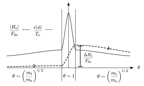
Figure 1: An illustration showing the nonadiabatic passing electron response for forward-going particles in the small-tail limit. At leading-order in the $\left(m_{\rm{e}}/m_{\rm{i}}\right)^{1/2}$ expansion, the mode frequency is determined by the response of ions and trapped electrons in the outer region ($\theta\sim 1$), by solving equations (31) and (39), with quasineutrality (66). The passing part of the electron distribution function $H_{\rm{e}}$ is propagated from left to right, via equation (63), starting with zero amplitude at $\theta=-\infty$, receiving an impulse $\Delta H_{\rm{e}}$ from the potential $\phi$ in the outer region (see equation (67)), and finally, carrying that amplitude into the inner region ($\theta\sim\left({m_{\rm{i}}}/{m_{\rm{e}}}\right)^{1/2}$). In the inner region, the trapped electron response may be determined with equation (64), and the electron response determines $\phi$, via quasineutrality (70).

The small correction $H_{{\rm{e}},{\scriptsize\rm{outer}}}^{(1)}$ from passing electrons does not enter in the leading-order eigenvalue problem, equation (66). As a result, in small-tail modes the nonadiabatic passing electron response is a “cosmetic” feature that does not contribute to determining the basic properties of the mode. Nonetheless, observable electron tails can develop in $k_{r}\rho_{\rm{th,e}}\sim 1$ regions ($\theta\sim\left({m_{\rm{i}}}/{m_{\rm{e}}}\right)^{1/2}$). We illustrate this in figure 1. The mode is decomposed into three regions: $\theta\sim 1$, and $|\theta|\sim\left({m_{\rm{i}}}/{m_{\rm{e}}}\right)^{1/2}$ for $\theta>0$ and $\theta<0$. Forward-going passing electrons travel through the $\theta\sim 1$ region, receiving an impulse

$${\Delta H_{\rm{e}}=\int^{\infty}_{-\infty}\frac{1}{v_{\|}\bm{b}\!\cdot\!\nabla\theta^{\prime}}\left(C_{\rm{ee}}\left[H_{{\rm{e}},{\scriptsize\rm{outer}}}^{(0)}\right]-{\rm{i}}\left(\omega_{\ast,{\rm{e}}}-\omega^{(0)}\right)\frac{e\phi_{{\scriptsize\rm{outer}}}^{(0)}}{T_{\rm{e}}}F_{0e}\right)d\theta^{\prime}}$$ (67)

from the electrostatic potential $\phi_{{\scriptsize\rm{outer}}}$. The matching condition for the electron nonadiabatic response in the $\theta\sim\left({m_{\rm{i}}}/{m_{\rm{e}}}\right)^{1/2}$ region $H_{{\rm{e}},{\scriptsize\rm{inner}}}$ is obtained from the jump condition (67) by demanding that the passing electron distribution function is continuous across the boundary between the outer and inner regions, i.e.,

$$H_{{\rm{e}},{\scriptsize\rm{outer}}}^{(1)}(\theta=\pm\infty)=H_{{\rm{e}},{\scriptsize\rm{inner}}}^{(0)}(\chi=0^{\pm}),{\rm{~{}for~{}}}0\leq\lambda B_{\rm max}\leq 1.$$ (68)

Combining equations (42), (67) and (68), we find that the matching condition for solving for the passing electron response in the small-tails limit is

$$H_{{\rm{e}},{\scriptsize\rm{inner}}}^{(0)}(\chi=0^{+})=H_{{\rm{e}},{\scriptsize\rm{inner}}}^{(0)}(\chi=0^{-})+\Delta H_{\rm{e}},$$ (69)

valid for both $\sigma\pm 1$. Once $\phi_{{\scriptsize\rm{outer}}}^{(0)}$ and $\omega^{(0)}$ are determined, we can self-consistently obtain the electron tails associated with a small-tail mode by solving the inner region equations (63) and (64) for the nonadiabatic response of passing electrons and trapped electrons, respectively, subject to the jump condition (69) at $\chi=0$. This obtains the functional $H_{{\rm{e}},{\scriptsize\rm{inner}}}^{(0)}=H_{{\rm{e}},{\scriptsize\rm{inner}}}^{(0)}[\phi_{{\scriptsize\rm{inner}}}^{(0)},\phi_{{\scriptsize\rm{outer}}}^{(0)},\omega^{(0)}]$. Finally, we impose quasineutrality in the inner region to obtain a relation for $\phi_{{\scriptsize\rm{inner}}}^{(0)}$ in terms of the jump over $\phi_{{\scriptsize\rm{outer}}}^{(0)}$, using the leading-order equation

$$\left(\frac{Z_{\rm{i}}T_{\rm{e}}}{T_{\rm{i}}}+1\right)\frac{e\phi_{{\scriptsize\rm{inner}}}^{(0)}}{T_{\rm{e}}}=-\int\exp{\left[{\rm{i}}\lambda_{{\rm{e}}}\chi\right]}J^{(0)}_{0{\rm{e}}}\frac{H_{{\rm{e}},{\scriptsize\rm{inner}}}^{(0)}}{n_{\rm{e}}}\;d^{3}\bm{v},$$ (70)

where we have used that the ion contribution to quasineutrality is small, cf. equation (58).

We obtain an estimate for the size of $\phi_{{\scriptsize\rm{inner}}}^{(0)}$ by noting that the impulse (67) sets the natural size of $H_{{\rm{e}},{\scriptsize\rm{inner}}}$ compared to the size of the potential in the outer region:

$$H_{{\rm{e}},{\scriptsize\rm{inner}}}\sim\Delta H_{\rm{e}}\sim\left(\frac{m_{\rm{e}}}{m_{\rm{i}}}\right)^{1/2}\frac{e\phi_{{\scriptsize\rm{outer}}}}{T_{\rm{e}}}{F_{0e}}.$$ (71)

Combining this estimate with equation (70), we find that the electrostatic potential in the inner region $\phi_{{\scriptsize\rm{inner}}}$ is of size

$$\frac{e\phi_{{\scriptsize\rm{inner}}}}{T_{\rm{e}}}\sim\left(\frac{m_{\rm{e}}}{m_{\rm{i}}}\right)^{1/2}\frac{e\phi_{{\scriptsize\rm{outer}}}}{T_{\rm{e}}}.$$ (72)

4.4 Modes with dominant electron tails

We now turn to the novel class of modes identified in this paper. To obtain a “large-tail” mode in the $\left(m_{\rm{e}}/m_{\rm{i}}\right)^{1/2}\rightarrow 0$ limit, we assume that the leading-order nonadiabatic passing electron response is nonzero in the outer region, i.e.,

$$\frac{H_{{\rm{e}},{\scriptsize\rm{outer}}}}{F_{0e}}\sim\frac{e\phi_{{\scriptsize\rm{outer}}}}{T_{\rm{e}}}.$$ (73)

We recall from section 4.1.2 that $H_{{\rm{e}},{\scriptsize\rm{outer}}}^{(0)}$ is a constant in $\theta$, and is independent of the ion response and the trapped electron response in the outer region. As a consequence, in the ordering (73) we may solve the leading-order equations (63) and (64) for $H^{(0)}_{{\rm{e}}}$ in the inner region with the boundary condition that

$$H_{{\rm{e}},{\scriptsize\rm{inner}}}^{(0)}(\chi=0^{-})=H_{{\rm{e}},{\scriptsize\rm{inner}}}^{(0)}(\chi=0^{+}).$$ (74)

Imposing quasineutrality via equation (70) results in an eigenvalue problem for $\phi_{{\scriptsize\rm{inner}}}^{(0)}$ and $\omega^{(0)}$. We illustrate the mode structure in the large-tail ordering in figure 2.

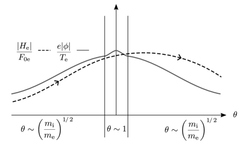
Figure 2: An illustration showing the nonadiabatic passing electron response for forward-going particles in the large-tail limit. In this limit, the electron response in the inner region ($\theta\sim\left({m_{\rm{i}}}/{m_{\rm{e}}}\right)^{1/2}$) determines the mode frequency to leading order in the $\left(m_{\rm{e}}/m_{\rm{i}}\right)^{1/2}$ expansion: we solve equations (63) and (64) for the passing and trapped electron response, respectively, subject to quasineutrality (70). In the outer region, the electron response $H_{\rm{e}}$ is approximately constant, and ions respond passively, without modifying the frequency to leading order.

Note in particular that the nonadiabatic passing electron response changes by only a small ($\left(m_{\rm{e}}/m_{\rm{i}}\right)^{1/2}$) amount over the $\theta\sim 1$ region. As a consequence of the ordering (73), and the boundary condition (74), we find that the electrostatic potential in the inner region has no mass ratio scaling with respect to the electrostatic potential in the outer region, i.e.,

$$\frac{e\phi_{{\scriptsize\rm{inner}}}}{T_{\rm{e}}}\sim\frac{e\phi_{{\scriptsize\rm{outer}}}}{T_{\rm{e}}}.$$ (75)

An interesting corollary of these arguments is that the leading order complex frequency $\omega^{(0)}$ of a large-tail mode should be independent of $\theta_{0}$.

Finally, in a large-tail mode the role of the nonadiabatic ion response (and nonadiabatic trapped electron response for $\theta\sim 1$) is to modify the leading-order mode structure at $\theta\sim 1$ without modifying the frequency $\omega^{(0)}$. To see this, note that equations (63), (64), and (70) determine the frequency $\omega^{(0)}$. However, $\phi_{{\scriptsize\rm{outer}}}^{(0)}$ is not yet determined: in the $\theta\sim 1$ region only the nonadiabatic density due to passing electrons $\delta\!n^{(0)}_{\rm{e,passing}}$ is fixed by the passing electron tails. To obtain $\phi_{{\scriptsize\rm{outer}}}^{(0)}$, we solve equation (31) for the nonadiabatic ion response $h_{{\rm{i}},{\scriptsize\rm{outer}}}^{(0)}=h_{{\rm{i}},{\scriptsize\rm{outer}}}^{(0)}[\phi_{{\scriptsize\rm{outer}}}^{(0)},\omega^{(0)}]$, and equation (39) for the nonadiabatic trapped electron response $H_{{\rm{e}},{\scriptsize\rm{outer-trapped}}}^{(0)}=H_{{\rm{e}},{\scriptsize\rm{outer-trapped}}}^{(0)}[\phi_{{\scriptsize\rm{outer}}}^{(0)},\omega^{(0)}]$, where we have indicated that $h_{{\rm{i}},{\scriptsize\rm{outer}}}^{(0)}$ and $H_{{\rm{e}},{\scriptsize\rm{outer-trapped}}}^{(0)}$ are functionals of $\phi_{{\scriptsize\rm{outer}}}^{(0)}$ and functions of $\omega^{(0)}$. We then use $\theta\sim 1$ quasineutrality, equation (66), to obtain $\phi_{{\scriptsize\rm{outer}}}^{(0)}$ as a function of $\delta\!n^{(0)}_{\rm{e,passing}}$. The role of the nonadiabatic ion response (and the nonadiabatic trapped electron response) is to modify the response of the electrostatic potential $\phi_{{\scriptsize\rm{outer}}}^{(0)}$ to an input $\omega^{(0)}$ and $\delta\!n^{(0)}_{\rm{e,passing}}$.

4.5 Relating the derivation of gyrokinetics to the derivation of the transit and bounce averaged equations for the electron response

We conclude this section on collisionless physics by commenting on the relationship between the derivation of gyrokinetics and the derivation of the transit and bounce averaged equations for the electron response in the inner region. We note that in the derivation of the gyrokinetic equation the change of variables from $({\bm{r}},\varepsilon,\lambda,\gamma)$ to $({\bm{R}},\varepsilon,\lambda,\gamma)$ introduces the finite-Larmor-radius phase $\exp{\left[{\rm{i}}\bm{k}_{\perp}\cdot\bm{\rho}_{s}\right]}$ into the kinetic equation. The $\gamma$ dependence in the kinetic equation can be removed by a gyroaverage $\left\langle{\cdot}\right\rangle^{\gamma}$ because the field $\phi({\bm{r}})$ has no dependence on the gyrophase $\gamma$, and the finite-Larmor-radius phases are converted into a Bessel function $J_{0}(b_{s})$ by the gyroaverage $\left\langle{\cdot}\right\rangle^{\gamma}$. In the derivation of the equations for the electron response in the inner region, equations (63) and (64), we find that the leading-order electron distribution function $H^{(0)}_{{\rm{e}}}=H^{(0)}_{{\rm{e}}}(\chi,\varepsilon,\lambda,\sigma)$ is independent of $\theta$, and the phase $\exp{\left[-{\rm{i}}\lambda_{{\rm{e}}}\chi\right]}$ keeps track of the electron drift-orbit motion. However, the potential $\phi^{(0)}=\phi^{(0)}(\theta,\chi)$ has a nontrivial dependence on $\theta$. This can be observed by inspecting the inner region quasineutrality relation, equation (70), where we see that velocity-space structure in $H^{(0)}_{{\rm{e}}}$ influences the $\theta$ structure of $\phi^{(0)}$. As a consequence, we may not directly remove $\theta$ when solving the system of equations (63), (64), and (70).

5 Long-wavelength collisional electrostatic modes in the $\left(m_{\rm{e}}/m_{\rm{i}}\right)^{1/2}\rightarrow 0$ limit

In this section, we present reduced model equations for long-wavelength, collisional, electrostatic modes in the $\left(m_{\rm{e}}/m_{\rm{i}}\right)^{1/2}\rightarrow 0$ limit. We define the collisional limit to be the limit (2). In the collisional limit, the scale of the mode in extended ballooning angle $\chi$ is set by the balance between parallel and perpendicular classical and neoclassical diffusion terms appearing in the equations for the mode. This means that we expect a balance

$$\frac{v_{\rm{th,e}}^{2}}{q^{2}R_{0}^{2}\nu_{\rm{ee}}}\frac{\partial^{2}}{\partial\chi^{2}}\sim\nu_{\rm{ee}}k_{y}^{2}\rho_{\rm{th,e}}^{2}\chi^{2}.$$ (76)

We can rearrange the balance (76) to give an estimate for the size of $\chi$. We find that

$$\chi\sim\left(\frac{qR_{0}\nu_{\rm{ee}}}{v_{\rm{th,e}}}\right)^{-1/2}\left(\frac{m_{\rm{i}}}{m_{\rm{e}}}\right)^{1/4}.$$ (77)

For the collisional ordering of $qR_{0}\nu_{\rm{ee}}/v_{\rm{th,e}}\sim 1$, the scale of the electron tail is $\chi\sim\left({m_{\rm{i}}}/{m_{\rm{e}}}\right)^{1/4}$. As expected, the “collisionless” ordering of $qR_{0}\nu_{\rm{ee}}/v_{\rm{th,e}}\sim\left(m_{\rm{e}}/m_{\rm{i}}\right)^{1/2}$ in the estimate (77) yields the scale $\chi\sim\left({m_{\rm{i}}}/{m_{\rm{e}}}\right)^{1/2}$. In section 5.1.4, we demonstrate that there is a continuous transition between the collisional and the collisionless limits.

We obtain the equations for the response of ions and electrons in a $k_{y}\rho_{\rm{th,i}}\sim 1$ mode with a $\theta\sim 1$ outer region, and a $\theta\sim\left({m_{\rm{i}}}/{m_{\rm{e}}}\right)^{1/4}$ inner region. Although the details of the equations obtained here are different to the collisionless case, the final result is qualitatively similar: two types of modes exist, large-tail modes driven by the nonadiabatic electron response at $\theta\sim\left({m_{\rm{i}}}/{m_{\rm{e}}}\right)^{1/4}$ scales, and conventional small-tail modes driven by the ion response at $\theta\sim 1$ scales. Note that in the collisional limit, trapped electrons cannot drive an instability because their orbits are disrupted by collisions. In order to motivate the $\left({m_{\rm{e}}}/{m_{\rm{i}}}\right)^{1/4}$ expansion, we first present the equations in the $\theta\gg 1$ region. As in the collisionless case, the equations that we obtain in the $\theta\gg 1$ region are common to both classes of mode. The two different classes of mode are distinguished by the boundary matching at $\theta\sim 1$. Section 5.3 provides a description of the boundary matching between the outer and inner regions for the small-tail mode, in addition to a plenary summary for how to solve the small-tail mode equations. Finally, section 5.4 provides a description of the boundary matching between the outer and inner regions for the large-tail mode, and a plenary summary for how to solve the large-tail mode equations.

5.1 Collisional inner solution – $\theta\sim\left({m_{\rm{i}}}/{m_{\rm{e}}}\right)^{1/4}$ – $k_{r}\rho_{\rm{th,e}}\sim\left({m_{\rm{e}}}/{m_{\rm{i}}}\right)^{1/4}$

To treat the fine radial scales of the collisional inner region, we introduce an additional coordinate $\chi$ measuring distance along the magnetic field line, via the substitutions (43) and (44). The coordinate $\theta$ will measure $2\pi$ periodic variation, whereas $\chi\sim\left({m_{\rm{i}}}/{m_{\rm{e}}}\right)^{1/4}$ is an extended ballooning angle for the envelope of the mode. Refer to the discussion in section 4.2 for the details of the substitution in geometric quantities (equations (45)-(49)); and the modifications to the boundary conditions on the electron distribution function (equations (50) and (51)). In the collisional limit, we can note the similarity of structure of the derivation of the inner region equations to the treatment of resistive ballooning modes and semi-collisional tearing modes in toroidal geometry, see, for example, [38] and [39], respectively.

To proceed, we expand electrostatic potential $\phi$, distribution functions $h_{s}$, and frequency $\omega$ in powers of $\left(m_{\rm{e}}/m_{\rm{i}}\right)^{1/4}$, i.e., for the potential we expand

$$\phi{}=\phi^{(0)}+\phi^{(1/2)}+\phi^{(1)}+\Or\left(\left(\frac{m_{\rm{e}}}{m_{\rm{i}}}\right)^{3/4}\phi\right),$$ (78)

with $\phi^{(n)}\sim\left(m_{\rm{e}}/m_{\rm{i}}\right)^{n/2}\phi$. Identical expansions are made for $h_{s}$ and $\omega$, again taking $h_{s}{}^{(n)}\sim\left(m_{\rm{e}}/m_{\rm{i}}\right)^{n/2}(e\phi{}/T_{\rm{e}})F_{0s}$ and $\omega^{(n)}\sim\left(m_{\rm{e}}/m_{\rm{i}}\right)^{n/2}\omega$. As in the collisionless case, to solve for the electron response, we use the modified electron distribution function $H_{\rm{e}}$, defined by equation (25), rather than the usual distribution function $h_{{\rm{e}}}$. We leave the relative size of the fluctuations in the outer and inner regions to be determined by the matching in sections 5.3 and 5.4.

5.1.1 Ion response in the collisional inner region.

Before considering the electron response, we first comment on the ion response in the inner region in the collisional limit. The analysis proceeds almost identically to the analysis presented in section 4.2.1 for the ion response in the collisionless limit. For $\nu_{\rm{ii}}/\omega\sim 1$ and $\chi\sim\left({m_{\rm{i}}}/{m_{\rm{e}}}\right)^{1/4}$, we find that the leading-order equation for the ion response has the same form as equation (53), apart from the fact that the radial magnetic drift term is neglected. This observation allows us to obtain an estimate for $h_{{\rm{i}}}{}^{(0)}$: $h_{{\rm{i}}}{}^{(0)}/F_{0i}\sim\chi^{-5/2}\;e\phi^{(0)}/T_{\rm{e}}$, where we have employed that $J_{0{\rm{i}}}\sim\Or\left(\chi^{-1/2}\right)$ for $\chi\gg 1$. This estimate for $h_{{\rm{i}}}{}^{(0)}$ yields estimates for the ion nonadiabatic density $\delta\!n^{(0)}_{\rm{i}}$ and the ion mean velocity $\delta\!\bm{u}^{(0)}_{{\rm{i}}}$, required for the electron-ion piece of the electron collision operator,

$$\frac{\delta\!n^{(0)}_{\rm{i}}}{n_{\rm{i}}}\sim\frac{\delta\!\bm{u}^{(0)}_{{\rm{i}}}}{v_{\rm{th,i}}}\sim\left(\frac{m_{\rm{e}}}{m_{\rm{i}}}\right)^{3/4}\frac{e\phi^{(0)}{}}{T_{\rm{e}}}\ll\frac{e\phi^{(0)}{}}{T_{\rm{e}}},$$ (79)

where we have used that $J_{0{\rm{i}}}\sim J_{1{\rm{i}}}\sim\Or\left(\left({m_{\rm{e}}}/{m_{\rm{i}}}\right)^{1/8}\right)$. The estimate (79) shows that the nonadiabatic ion response has no leading-order contribution to the mode evolution in the inner region.

5.1.2 Electron response in the collisional inner region.

The calculation of the electron response in the collisional inner region has a structure that is reminiscent of neoclassical transport theory. The leading-order equation constrains the leading-order electron distribution function to be a perturbed Maxwellian with no flows. The first-order equation takes the form of a Spitzer-Härm problem [41, 31, 32]. Physically, the first-order terms control the self-consistent parallel flows that result from the leading-order perturbations. The second-order equation governs the time evolution of the leading-order fluctuations. A poloidal angle average

$$\left\langle{\cdot}\right\rangle^{\theta}=\int^{\pi}_{-\pi}\left(\cdot\right)\;\frac{d\theta}{\bm{B}\cdot\nabla\theta}{\left/\int^{\pi}_{-\pi}\frac{d\theta}{\bm{B}\cdot\nabla\theta}\right.}$$ (80)

of the density and temperature velocity moments of the second-order equation yield transport equations for the electron density and temperature fluctuations, closing the system of equations. In this section, we give the forms of the transport equations in the $\left({m_{\rm{e}}}/{m_{\rm{i}}}\right)^{1/4}\rightarrow 0$ limit, with $qR_{0}\nu_{\rm{ee}}/v_{\rm{th,e}}\sim 1$. The full details of the calculation are contained in B.

The leading order equation for the electron response in the inner region is a balance between parallel streaming in the periodic coordinate $\theta$ and collisions:

$$v_{\|}\bm{b}\!\cdot\!\nabla\theta\frac{\partial H^{(0)}_{{\rm{e}}}}{\partial\theta}=C_{\rm{ee}}\left[H^{(0)}_{{\rm{e}}}\right]+\mathcal{L}\left[H^{(0)}_{{\rm{e}}}\right].$$ (81)

To solve equation (81), in B we follow the standard H-theorem procedure [40, 32] to prove that $H^{(0)}_{{\rm{e}}}$ is a perturbed Maxwellian with no flow, i.e.,

$$\frac{H^{(0)}_{{\rm{e}}}}{F_{0e}}=\frac{\delta\!n^{(0)}_{\rm{e}}}{n_{\rm{e}}}+\frac{\delta\!T^{(0)}_{\rm{e}}}{T_{\rm{e}}}\left(\frac{\varepsilon}{T_{\rm{e}}}-\frac{3}{2}\right),$$ (82)

where the nonadiabatic density $\delta\!n^{(0)}_{\rm{e}}$ and temperature $\delta\!T^{(0)}_{\rm{e}}$ are constant in $\theta$, i.e.,

$$\delta\!n^{(0)}_{\rm{e}}=\delta\!n^{(0)}_{\rm{e}}(\chi),\quad{\rm{and}}\quad\delta\!T^{(0)}_{\rm{e}}=\delta\!T^{(0)}_{\rm{e}}(\chi).$$ (83)

To obtain evolution equations for $\delta\!n^{(0)}_{\rm{e}}$ and $\delta\!T^{(0)}_{\rm{e}}$, in B we go to second order in the expansion in $\left({m_{\rm{e}}}/{m_{\rm{i}}}\right)^{1/4}$.

Before writing down the transport equations, we consider the collisional inner-region quasineutrality relation. Using the the ordering (79), and the solution (82), with $J_{0{\rm{e}}}=1+\Or\left(\left(m_{\rm{e}}/m_{\rm{i}}\right)^{1/2}\right)$ and $\exp{\left[{\rm{i}}\lambda_{{\rm{e}}}(\chi-\theta_{0})\right]}=1+\Or\left(\left({m_{\rm{e}}}/{m_{\rm{i}}}\right)^{1/4}\right)$ for $\chi\sim\left({m_{\rm{i}}}/{m_{\rm{e}}}\right)^{1/4}$ and $k_{y}\rho_{\rm{th,i}}\sim 1$, we find that the leading-order quasineutrality relation is

$$\left(\frac{Z_{\rm{i}}T_{\rm{e}}}{T_{\rm{i}}}+1\right)\frac{e\phi^{(0)}}{T_{\rm{e}}}=-\int\frac{H^{(0)}_{{\rm{e}}}}{n_{\rm{e}}}\;d^{3}\bm{v}=-\frac{\delta\!n^{(0)}_{\rm{e}}}{n_{\rm{e}}}.$$ (84)

Equation (84) allows us to note that the electrostatic potential in the inner region is not a function of geometric angle $\theta$, i.e., $\phi^{(0)}=\phi^{(0)}(\chi)$. This is a significant simplification over the collisionless case (cf. equation (70)), where $\phi^{(0)}=\phi^{(0)}(\theta,\chi)$. This simplification arises in the collisional limit because, first, there is no distinction between trapped and passing particles; and second, the extent of the mode is shortened to $\chi\sim\left({m_{\rm{i}}}/{m_{\rm{e}}}\right)^{1/4}$, meaning that finite-Larmor-radius and finite-orbit-width effects do not enter at leading order.

The final transport equations for $\delta\!n^{(0)}_{\rm{e}}$ and $\delta\!T^{(0)}_{\rm{e}}$ are are most clearly written in a form where the terms admit simple physical interpretations. We have a continuity equation

$$\left\langle{\bm{b}\!\cdot\!\nabla\theta}\right\rangle^{\theta}\frac{\partial\overline{\delta\!u}_{\|}}{\partial\chi}+{\rm{i}}\left\langle{\omega_{D}}\right\rangle^{\theta}\left(\frac{\delta\!n^{(0)}_{\rm{e}}}{n_{\rm{e}}}+\frac{\delta\!T^{(0)}_{\rm{e}}}{T_{\rm{e}}}\right)-{\rm{i}}\omega^{(0)}\frac{\delta\!n^{(0)}_{\rm{e}}}{n_{\rm{e}}}-{\rm{i}}k_{y}\hat{s}\hat{\kappa}\chi\left(\frac{\overline{\delta\!\Gamma}_{\rm C}}{n_{\rm{e}}}+\frac{\overline{\delta\!\Gamma}_{\rm N}}{n_{\rm{e}}}\right)$$ (85)

$$=-{\rm{i}}(\omega^{n}_{\ast,{\rm{e}}}-\omega^{(0)})\frac{e\phi^{(0)}}{T_{\rm{e}}},$$

and a temperature equation

$$\left\langle{\bm{b}\!\cdot\!\nabla\theta}\right\rangle^{\theta}\frac{\partial}{\partial\chi}\left(\frac{\overline{\delta\!q}_{\|}}{n_{\rm{e}}T_{\rm{e}}}+\overline{\delta\!u}_{\|}\right)+{\rm{i}}\left\langle{\omega_{D}}\right\rangle^{\theta}\left(\frac{\delta\!n^{(0)}_{\rm{e}}}{n_{\rm{e}}}+\frac{7}{2}\frac{\delta\!T^{(0)}_{\rm{e}}}{T_{\rm{e}}}\right)-{\rm{i}}\frac{3}{2}\omega^{(0)}\frac{\delta\!T^{(0)}_{\rm{e}}}{T_{\rm{e}}}$$

$$-{\rm{i}}k_{y}\hat{s}\hat{\kappa}\chi\left(\frac{\overline{\delta\!\Gamma}_{\rm C}}{n_{\rm{e}}}+\frac{\overline{\delta\!q}_{\rm C}}{n_{\rm{e}}T_{\rm{e}}}+\frac{\overline{\delta\!\Gamma}_{\rm N}}{n_{\rm{e}}}+\frac{\overline{\delta\!q}_{\rm N}}{n_{\rm{e}}T_{\rm{e}}}\right)=-{\rm{i}}\frac{3}{2}\omega^{n}_{\ast,{\rm{e}}}\eta_{\rm{e}}\frac{e\phi^{(0)}}{T_{\rm{e}}}.$$ (86)

The physical interpretations of the terms in equations (85) and (86) are the following, from left to right: parallel diffusion, magnetic (precession) drifts within the flux surface, time evolution, classical perpendicular diffusion, neoclassical perpendicular diffusion, and drives by equilibrium gradients. To write equations (85) and (86), we have defined the effective parallel velocity and effective parallel heat flux,

$$\overline{\delta\!u}_{\|}=\frac{1}{\left\langle{\bm{b}\!\cdot\!\nabla\theta}\right\rangle^{\theta}}\left\langle{\frac{\bm{b}\!\cdot\!\nabla\theta}{n_{\rm{e}}}\int v_{\|}(H^{(1/2)}_{{\rm{e}}}+{\rm{i}}\lambda_{{\rm{e}}}\chi H^{(0)}_{{\rm{e}}})\;d^{3}\bm{v}}\right\rangle^{\theta},$$ (87)

and

$$\overline{\delta\!q}_{\|}=\frac{1}{\left\langle{\bm{b}\!\cdot\!\nabla\theta}\right\rangle^{\theta}}\left\langle{\bm{b}\!\cdot\!\nabla\theta\int v_{\|}\left(\varepsilon-\frac{5T_{\rm{e}}}{2}\right)(H^{(1/2)}_{{\rm{e}}}+{\rm{i}}\lambda_{{\rm{e}}}\chi H^{(0)}_{{\rm{e}}})\;d^{3}\bm{v}}\right\rangle^{\theta},$$ (88)

respectively, the thermal magnetic precession drift

$$\omega_{D}=\frac{k_{\alpha}v_{\rm{th,e}}^{2}}{2\Omega_{\rm{e}}}\bm{b}\times\left(\bm{b}\cdot\nabla\bm{b}+\frac{\nabla B}{B}\right)\cdot\left(\nabla\alpha+\theta\nabla q\right),$$ (89)

the fluctuating perpendicular fluxes: the classical particle flux

$$\overline{\delta\!\Gamma}_{\rm C}={\rm{i}}\left\langle{\int\nabla r\cdot\bm{\rho}_{e}\;\mathcal{C}\left[\bm{k}^{(0)}_{\perp}\cdot\bm{\rho}_{e}\;H^{(0)}_{{\rm{e}}}\right]\;d^{3}\bm{v}}\right\rangle^{\theta},$$ (90)

the classical heat flux

$$\overline{\delta\!q}_{\rm C}={\rm{i}}\left\langle{\int\left(\varepsilon-\frac{5T_{\rm{e}}}{2}\right)\nabla r\cdot\bm{\rho}_{e}\;\mathcal{C}\left[\bm{k}^{(0)}_{\perp}\cdot\bm{\rho}_{e}\;H^{(0)}_{{\rm{e}}}\right]\;d^{3}\bm{v}}\right\rangle^{\theta},$$ (91)

the neoclassical particle flux

$$\overline{\delta\!\Gamma}_{\rm N}=-\left\langle{\frac{I}{\Omega_{\rm{e}}}\frac{dr}{d\psi}\int v_{\|}\;\mathcal{C}\left[H^{(1/2)}_{{\rm{e}}}+{\rm{i}}\lambda_{{\rm{e}}}\chi H^{(0)}_{{\rm{e}}}-H_{\rm{SH}}\right]\;d^{3}\bm{v}}\right\rangle^{\theta},$$ (92)

and the neoclassical heat flux

$$\overline{\delta\!q}_{\rm N}=-\left\langle{\frac{I}{\Omega_{\rm{e}}}\frac{dr}{d\psi}\int\left(\varepsilon-\frac{5T_{\rm{e}}}{2}\right)v_{\|}\;\mathcal{C}\left[H^{(1/2)}_{{\rm{e}}}+{\rm{i}}\lambda_{{\rm{e}}}\chi H^{(0)}_{{\rm{e}}}-H_{\rm{SH}}\right]\;d^{3}\bm{v}}\right\rangle^{\theta}.$$ (93)

To obtain $\overline{\delta\!u}_{\|}$, $\overline{\delta\!q}_{\|}$, $\overline{\delta\!\Gamma}_{\rm N}$ and $\overline{\delta\!q}_{\rm N}$ we require the $\left({m_{\rm{e}}}/{m_{\rm{i}}}\right)^{1/4}$ small distribution functions $H_{\rm{SH}}$ and $H^{(1/2)}_{{\rm{e}}}$. The distribution function $H_{\rm{SH}}$ is determined by solving the Spitzer-Härm problem [41, 31, 32]

$$v_{\|}\bm{b}\!\cdot\!\nabla\theta\frac{\partial H^{(0)}_{{\rm{e}}}}{\partial\chi}=\mathcal{C}[H_{\rm{SH}}],$$ (94)

whereas $H^{(1/2)}_{{\rm{e}}}$ is determined by solving the first-order electron equation

$$v_{\|}\bm{b}\!\cdot\!\nabla\theta\frac{\partial H^{(1/2)}_{{\rm{e}}}}{\partial\theta}=\mathcal{C}\left[H^{(1/2)}_{{\rm{e}}}+{\rm{i}}\lambda_{{\rm{e}}}\chi H^{(0)}_{{\rm{e}}}-H_{\rm{SH}}\right].$$ (95)

In general, equation (95) is not solvable analytically. To maximise the physical insight from the calculation, we subsequently solve equation (95) in the subsidiary limits of large and small collisionality.

The classical fluxes $\overline{\delta\!\Gamma}_{\rm C}$ and $\overline{\delta\!q}_{\rm C}$ are due to Larmor orbits being interupted by collisions, and can be evaluated for arbitrary $qR_{0}\nu_{\rm{ee}}/v_{\rm{th,e}}$ [32, 31]. We use the results of D to write down the classical particle flux $\overline{\delta\!\Gamma}_{\rm C}$ and classical heat flux $\overline{\delta\!q}_{\rm C}$. We use result (207) to find that

$$\frac{\overline{\delta\!\Gamma}_{\rm C}}{n_{\rm{e}}}={\rm{i}}k_{y}\hat{s}\hat{\kappa}\chi\frac{\nu_{\rm{ei}}\overline{\rho}_{\rm{th,e}}^{2}}{2}\left\langle{\overline{B}^{2}\frac{|\nabla r|^{2}}{B^{2}}}\right\rangle^{\theta}\left(\frac{\delta\!n^{(0)}_{\rm{e}}}{n_{\rm{e}}}-\frac{1}{2}\frac{\delta\!T^{(0)}_{\rm{e}}}{T_{\rm{e}}}\right),$$ (96)

where we have used that $\bm{k}^{(0)}_{\perp}=-k_{\alpha}(dq/dr)\chi\nabla r=-k_{y}\hat{s}\hat{\kappa}\chi\nabla r$, with $\overline{\rho}_{\rm{th,e}}=v_{\rm{th,e}}/\overline{\Omega}_{\rm{e}}$, $\overline{\Omega}_{\rm{e}}=-e\overline{B}/m_{{\rm{e}}}c$, and $\overline{B}=\left\langle{B}\right\rangle^{\theta}$. Similarly, we use the results (208) and (222) to find that

$$\frac{\overline{\delta\!q}_{\rm C}}{n_{\rm{e}}T_{\rm{e}}}={\rm{i}}k_{y}\hat{s}\hat{\kappa}\chi\frac{\nu_{\rm{ei}}\overline{\rho}_{\rm{th,e}}^{2}}{2}\left\langle{\overline{B}^{2}\frac{|\nabla r|^{2}}{B^{2}}}\right\rangle^{\theta}\left(\left(\frac{7}{4}+\frac{\sqrt{2}}{Z_{\rm{i}}}\right)\frac{\delta\!T^{(0)}_{\rm{e}}}{T_{\rm{e}}}-\frac{3}{2}\frac{\delta\!n^{(0)}_{\rm{e}}}{n_{\rm{e}}}\right),$$ (97)

where we have used that $\nu_{\rm{ee}}/\nu_{\rm{ei}}=1/Z_{\rm{i}}$.

The mode evolution equations for the density and the temperature, equations (85) and (86), respectively, have the promised structure: the envelope of the mode is controlled by the combination of the finite-orbit-width and finite-Larmor-radius perpendicular diffusion, and parallel diffusion. The perpendicular diffusion terms scale as $\nu_{\rm{ei}}(k_{y}\rho_{\rm{th,e}})^{2}\chi^{2}$, whereas equations (95), (87) and (88) show implicitly that the parallel diffusion terms scale as $(v_{\rm{th,e}}^{2}/\nu_{\rm{ei}}q^{2}R_{0}^{2}){\partial^{2}}/{\partial\chi^{2}}$. This result justifies the initial ordering (77) and the discussion in section 5.1. To obtain explicit analytical forms for all terms in the transport equations (85) and (86), we consider the $qR_{0}\nu_{\rm{ee}}/v_{\rm{th,e}}\gg 1$ (Pfirsh-Schlüter) regime in the next section. To demonstrate the transition between the collisionless and collisional regimes, we consider the $qR_{0}\nu_{\rm{ee}}/v_{\rm{th,e}}\ll 1$ (banana-plateau) regime in section 5.1.4.

5.1.3 Parallel flows and perpendicular diffusion in the subsidiary limit of $qR_{0}\nu_{\rm{ee}}/v_{\rm{th,e}}\gg 1$ – the Pfirsh-Schlüter regime.

In order to obtain the analytical form of the transport equations in the subsidiary limit $qR_{0}\nu_{\rm{ee}}/v_{\rm{th,e}}\gg 1$, we must solve equation (95) to obtain approximate solutions for $H^{(1/2)}_{{\rm{e}}}$. Using the results of E, we can write down the effective parallel velocity, parallel heat flux, and perpendicular diffusion terms that appear in the transport equations (85) and (86) in the $qR_{0}\nu_{\rm{ee}}/v_{\rm{th,e}}\gg 1$ limit. We find that

$$\frac{\overline{\delta\!u}_{\|}}{v_{\rm{th,e}}}=-\frac{v_{\rm{th,e}}}{2\nu_{\rm{ei}}}\frac{(\left\langle{\bm{B}\cdot\nabla\theta}\right\rangle^{\theta})^{2}}{\left\langle{\bm{b}\!\cdot\!\nabla\theta}\right\rangle^{\theta}\left\langle{B^{2}}\right\rangle^{\theta}}\left[1.97\frac{\partial}{\partial\chi}\left(\frac{\delta\!n^{(0)}_{\rm{e}}}{n_{\rm{e}}}\right)+3.37\frac{\partial}{\partial\chi}\left(\frac{\delta\!T^{(0)}_{\rm{e}}}{T_{\rm{e}}}\right)\right]$$ (98)

$$+\frac{{\rm{i}}}{2}\frac{k_{y}\overline{\rho}_{\rm{th,e}}\hat{\kappa}\hat{s}\chi}{\left\langle{\bm{b}\!\cdot\!\nabla\theta}\right\rangle^{\theta}}\overline{B}I\frac{dr}{d\psi}\left(\left\langle{\frac{\bm{B}\cdot\nabla\theta}{B^{2}}}\right\rangle^{\theta}-\frac{\left\langle{\bm{B}\cdot\nabla\theta}\right\rangle^{\theta}}{\left\langle{B^{2}}\right\rangle^{\theta}}\right)\left(\frac{\delta\!n^{(0)}_{\rm{e}}}{n_{\rm{e}}}+\frac{\delta\!T^{(0)}_{\rm{e}}}{T_{\rm{e}}}\right),$$

where we have used equation (246), with the numerical results (190) and (201) for the transport coefficients, assuming $Z_{\rm{i}}=1$. Similarly, using (247), we obtain the effective electron parallel heat flux

$$\frac{\overline{\delta\!q}_{\|}}{n_{\rm{e}}T_{\rm{e}}v_{\rm{th,e}}}=-\frac{5v_{\rm{th,e}}}{4\nu_{\rm{ei}}}\frac{(\left\langle{\bm{B}\cdot\nabla\theta}\right\rangle^{\theta})^{2}}{\left\langle{\bm{b}\!\cdot\!\nabla\theta}\right\rangle^{\theta}\left\langle{B^{2}}\right\rangle^{\theta}}\left[0.56\frac{\partial}{\partial\chi}\left(\frac{\delta\!n^{(0)}_{\rm{e}}}{n_{\rm{e}}}\right)+2.23\frac{\partial}{\partial\chi}\left(\frac{\delta\!T^{(0)}_{\rm{e}}}{T_{\rm{e}}}\right)\right]$$ (99)

$$+\frac{5{\rm{i}}}{4}\frac{k_{y}\overline{\rho}_{\rm{th,e}}\hat{\kappa}\hat{s}\chi}{\left\langle{\bm{b}\!\cdot\!\nabla\theta}\right\rangle^{\theta}}\overline{B}I\frac{dr}{d\psi}\left(\left\langle{\frac{\bm{B}\cdot\nabla\theta}{B^{2}}}\right\rangle^{\theta}-\frac{\left\langle{\bm{B}\cdot\nabla\theta}\right\rangle^{\theta}}{\left\langle{B^{2}}\right\rangle^{\theta}}\right)\frac{\delta\!T^{(0)}_{\rm{e}}}{T_{\rm{e}}}.$$

We note that the terms linear in $\chi$ in equations (98) and (99) arise from the radial magnetic drift, whereas the terms in ${\partial}/{\partial\chi}$ arise from the effective electric field generated by the leading-order electron response (cf. equation (143)).

The neoclassical particle flux $\overline{\delta\!\Gamma}_{\rm N}$ appearing in the nonadiabatic density transport equation, equation (85), can be evaluated using the result (250). We find that

$$\frac{\overline{\delta\!\Gamma}_{\rm N}}{n_{\rm{e}}}=-\frac{v_{\rm{th,e}}\overline{\rho}_{\rm{th,e}}}{2}I\frac{dr}{d\psi}\overline{B}\left(\frac{\left\langle{\bm{B}\cdot\nabla\theta}\right\rangle^{\theta}}{\left\langle{B^{2}}\right\rangle^{\theta}}-\left\langle{\frac{\bm{B}\cdot\nabla\theta}{B^{2}}}\right\rangle^{\theta}\right)\left(\frac{\partial}{\partial\chi}\left(\frac{\delta\!n^{(0)}_{\rm{e}}}{n_{\rm{e}}}\right)+\frac{\partial}{\partial\chi}\left(\frac{\delta\!T^{(0)}_{\rm{e}}}{T_{\rm{e}}}\right)\right)$$

$$+{\rm{i}}k_{y}\hat{s}\hat{\kappa}\chi\frac{\nu_{\rm{ei}}\overline{\rho}_{\rm{th,e}}^{2}}{2}\left(I\frac{dr}{d\psi}\right)^{2}\left(\left\langle{\frac{\overline{B}^{2}}{B^{2}}}\right\rangle^{\theta}-\frac{\overline{B}^{2}}{\left\langle{B^{2}}\right\rangle^{\theta}}\right)\left[0.67\frac{\delta\!n^{(0)}_{\rm{e}}}{n_{\rm{e}}}+0.11\frac{\delta\!T^{(0)}_{\rm{e}}}{T_{\rm{e}}}\right].$$ (100)

Similarly, the neoclassical heat flux $\overline{\delta\!q}_{\rm N}$ appearing in the temperature transport equation, equation (86), can be evaluated using the result (251). We find that

$$\frac{\overline{\delta\!q}_{\rm N}}{n_{\rm{e}}T_{\rm{e}}}=-\frac{5v_{\rm{th,e}}\overline{\rho}_{\rm{th,e}}}{4}I\frac{dr}{d\psi}\overline{B}\left(\frac{\left\langle{\bm{B}\cdot\nabla\theta}\right\rangle^{\theta}}{\left\langle{B^{2}}\right\rangle^{\theta}}-\left\langle{\frac{\bm{B}\cdot\nabla\theta}{B^{2}}}\right\rangle^{\theta}\right)\frac{\partial}{\partial\chi}\left(\frac{\delta\!T^{(0)}_{\rm{e}}}{T_{\rm{e}}}\right)$$ (101)

$$+{\rm{i}}k_{y}\hat{s}\hat{\kappa}\chi\frac{\nu_{\rm{ei}}\overline{\rho}_{\rm{th,e}}^{2}}{2}\left(I\frac{dr}{d\psi}\right)^{2}\left(\left\langle{\frac{\overline{B}^{2}}{B^{2}}}\right\rangle^{\theta}-\frac{\overline{B}^{2}}{\left\langle{B^{2}}\right\rangle^{\theta}}\right)\left[1.41\frac{\delta\!T^{(0)}_{\rm{e}}}{T_{\rm{e}}}-0.56\frac{\delta\!n^{(0)}_{\rm{e}}}{n_{\rm{e}}}\right].$$

Physically, equations (100) and (101) indicate that diffusive transport arises from the radial magnetic drift (note the terms linear in $\chi$).

We note that the scale of the extended tail, $\chi$, decreases with increasing $qR_{0}\nu_{\rm{ee}}/v_{\rm{th,e}}$. This is explicit in the estimate (77). Using (77), we can see that, for extreme collision frequencies where $qR_{0}\nu_{\rm{ee}}/v_{\rm{th,e}}\sim\left({m_{\rm{i}}}/{m_{\rm{e}}}\right)^{1/2}$, there is no separation between the scale of the electron tail and the scale of the geometric quantities: for such an extreme collisionality, $\chi\sim 1$. The fluid equations for this extreme regime are not examined in this paper.

5.1.4 The subsidiary limit of $qR_{0}\nu_{\rm{ee}}/v_{\rm{th,e}}\ll 1$ – the banana-plateau regime.

We now examine equation (95) in the subsidiary limit $qR_{0}\nu_{\rm{ee}}/v_{\rm{th,e}}\ll 1$. This discussion will enable us to demonstrate the smooth transition between the collisionless and collisional regimes. We will need to go to first-order in the subsidiary expansion of $qR_{0}\nu_{\rm{ee}}/v_{\rm{th,e}}\ll 1$, and so we expand

$${H^{(1/2)}_{{\rm{e}}}=H^{(1/2)}_{{\rm{e}},(0)}+H^{(1/2)}_{{\rm{e}},(1)}+\Or\left(\left(\frac{qR_{0}\nu_{\rm{ee}}}{v_{\rm{th,e}}}\right)^{2}H^{(1/2)}_{{\rm{e}},(0)}\right)},$$ (102)

where $H^{(1/2)}_{{\rm{e}},(0)}\sim{\rm{i}}\lambda_{{\rm{e}}}\chi H^{(0)}_{{\rm{e}}}\sim H_{\rm{SH}}$ and $H^{(1/2)}_{{\rm{e}},(n)}\sim\left(qR_{0}\nu_{\rm{ee}}/v_{\rm{th,e}}\right)^{n}H^{(1/2)}_{{\rm{e}},(0)}$. The leading-order form of equation (95) is

$$v_{\|}\bm{b}\!\cdot\!\nabla\theta\frac{\partial}{\partial\theta}\left(H^{(1/2)}_{{\rm{e}},(0)}\right)=0,$$ (103)

i.e., we learn that $H^{(1/2)}_{{\rm{e}},(0)}=H^{(1/2)}_{{\rm{e}},(0)}(\chi,\varepsilon,\lambda,\sigma)$. Going to first-order terms in the expansion of the drift-kinetic equation (95), we find that

$$v_{\|}\bm{b}\!\cdot\!\nabla\theta\frac{\partial}{\partial\theta}\left(H^{(1/2)}_{{\rm{e}},(1)}\right)=\mathcal{C}\left[H^{(1/2)}_{{\rm{e}},(0)}+{\rm{i}}\lambda_{{\rm{e}}}\chi H^{(0)}_{{\rm{e}}}-H_{\rm{SH}}\right].$$ (104)

We now impose the solvability condition that $H^{(1/2)}_{{\rm{e}},(1)}(\theta,\chi,\varepsilon,\lambda,\sigma)$ should be $2\pi$-periodic in $\theta$. We must treat the passing and trapped part of the velocity space independently. For passing particles we apply the transit average $\left\langle{\cdot}\right\rangle^{\rm{t}}$, defined in equation (62), to obtain

$$\left\langle{\mathcal{C}\left[H^{(1/2)}_{{\rm{e}},(0)}+{\rm{i}}\lambda_{{\rm{e}}}\chi H^{(0)}_{{\rm{e}}}-H_{\rm{SH}}\right]}\right\rangle^{\rm{t}}=0.$$ (105)

We note that equation (105) is a partial differential equation in $(\varepsilon,\lambda)$ at fixed $\chi$. For trapped particles we apply the bounce average $\left\langle{\cdot}\right\rangle^{\rm{b}}$, defined in equation (38), to obtain

$$\left\langle{\mathcal{C}\left[H^{(1/2)}_{{\rm{e}},(0)}\right]}\right\rangle^{\rm{b}}=0,$$ (106)

where we have used that ${\rm{i}}\lambda_{{\rm{e}}}\chi H^{(0)}_{{\rm{e}}}$ and $H_{\rm{SH}}$ are odd in $\sigma=v_{\|}/|v_{\|}|$, and therefore vanish under $\left\langle{\cdot}\right\rangle^{\rm{b}}$. The trapped particle bounce condition requires that

$$H^{(1/2)}_{{\rm{e}}}(\theta^{\pm}_{b},\sigma=1)=H^{(1/2)}_{{\rm{e}}}(\theta^{\pm}_{b},\sigma=-1),$$

and hence $H^{(1/2)}_{{\rm{e}},(0)}$ is even in $\sigma$, by virtue of being constant in $\theta$. In contrast, we can see from equation (105) that the passing particle response must be odd in $\sigma$. A Maxwellian solution to equation (106) is not valid, because of the change in the $\sigma$ symmetry of $H^{(1/2)}_{{\rm{e}},(0)}$ at the trapped-passing boundary, and hence we must have that $H^{(1/2)}_{{\rm{e}},(0)}=0$ for trapped particles. To obtain $H^{(1/2)}_{{\rm{e}},(0)}$ for passing particles, we must solve equation (105) subject to continuity in $H^{(1/2)}_{{\rm{e}},(0)}$ at the trapped-passing boundary.

In order to make progress analytically, it is necessary to expand in inverse aspect ratio $\epsilon=r/R_{0}\ll 1$, where $r$ is the minor radial coordinate of the flux surface of interest. We assume that the normalised collisionality

$$\nu_{\ast}=\frac{qR_{0}\nu_{\rm{ee}}}{\epsilon^{3/2}v_{\rm{th,e}}}\ll 1,$$ (107)

and assume that the equilibrium can be approximated by the solution with circular flux surfaces [30, 42]. Then, we can use the techniques of neoclassical theory [40, 32] to obtain $H^{(1/2)}_{{\rm{e}},(0)}$ to leading-order in $\epsilon$, and the velocity $\overline{\delta\!u}_{\|}$ and flux $\overline{\delta\!q}_{\|}$, and the neoclassical perpendicular diffusion terms to order $\epsilon^{1/2}$. These calculations are performed in F. We conclude that for $\nu_{\ast}\ll 1$ the electron parallel velocity and electron parallel heat flux have a diffusive character.

Finally, we comment on the smooth transition between the equations for the electron response in the collisionless and the collisional regimes. To obtain the mode transport equations (85) and (86) from the equations in the collisionless limit for the passing electron response, equation (63), and the trapped electron response, equation (64), we take the following steps: First, in equations (63) and (64), we take the electron collision frequency to be large compared to the ion transit frequency, i.e., $qR_{0}\nu_{\rm{ee}}/v_{\rm{th,i}}\gg 1$, and we take the extent of the ballooning mode to be small, with

$$1\ll\chi\sim\left(\frac{qR_{0}\nu_{\rm{ee}}}{v_{\rm{th,i}}}\right)^{-1/2}\left(\frac{m_{\rm{i}}}{m_{\rm{e}}}\right)^{1/2}\ll\left(\frac{m_{\rm{i}}}{m_{\rm{e}}}\right)^{1/2}.$$ (108)

Then, the leading-order equation for the electron response is

$$\mathcal{C}\left[H^{(0)}_{{\rm{e}}}\right]=0,$$ (109)

i.e., $H^{(0)}_{{\rm{e}}}$ is a perturbed Maxwellian with no flow, and with no dependence on $\theta$. Second, we collect terms of $\Or\left((qR_{0}\nu_{\rm{ee}}/v_{\rm{th,i}})^{-1/2}\right)$ in the subsidiary expansion, and obtain equations for the passing and trapped electron response of the form (105) and (106), respectively. Finally, we collect terms of $\Or\left((qR_{0}\nu_{\rm{ee}}/v_{\rm{th,i}})^{-1}\right)$ in the subsidiary expansion and obtain the transport equations for the nonadiabatic density and temperature, equations (85) and (86), respectively. The fact that the extent of the mode shortens when going from the collisionless to the collisional limits, according to the ordering (108), along with the Maxwellianisation of the distribution function by increasing interparticle collisions, cf. equation (109), ensures that the collisionless inner-region quasineutrality relation (70) takes the form of the collisional inner-region quasineutrality relation (84).

5.2 Collisional outer solution – $\theta\sim 1$ – $k_{r}\rho_{\rm{th,e}}\sim\left({m_{\rm{e}}}/{m_{\rm{i}}}\right)^{1/2}$

Just as in the collisionless case, the class of mode that we obtain in the collisional limit depends on the matching condition that we use to solve for the electron response in the inner region ($\theta\gg 1$) via equations (85) and (86). We obtain the matching conditions by considering the outer region ($\theta\sim 1$), and expanding in powers of $\left({m_{\rm{e}}}/{m_{\rm{i}}}\right)^{1/4}$, for consistency with the expansion in the inner region.

For the ions in the collisional ordering, we take $\nu_{\rm{ii}}\sim v_{\rm{th,i}}/qR$. As the electron mass does not appear in the ion gyrokinetic equation, no approximations are possible in this ordering and the gyrokinetic equation for the ions in the outer region is simply equation (4) with $s={\rm{i}}$. The nonadiabatic response of ions $h_{{\rm{i}}}$ contributes at leading-order to the potential $\phi$ in the outer region. As in the collisionless case (see equation (32)), the estimate for the size of the ion nonadiabatic density is $\delta\!n_{\rm{i}}/n_{\rm{i}}\sim e\phi/T_{\rm{e}}$.

5.3 Electron response in the outer region for small-tail modes.

In a collisional small-tail mode, the fluctuations must satisfy the ordering

$$\frac{H_{{\rm{e}},{\scriptsize\rm{inner}}}}{F_{0e}}\sim\frac{e\phi_{{\scriptsize\rm{inner}}}}{T_{\rm{e}}}\sim\frac{H_{{\rm{e}},{\scriptsize\rm{outer}}}}{F_{0e}}\ll\frac{e\phi_{{\scriptsize\rm{outer}}}}{T_{\rm{e}}},$$ (110)

so that the nonadiabatic electron response is subdominant to the nonadiabatic ion response in the outer region. This ordering will recover the ITG mode.

In this section, we present the matching condition necessary to solve for the electron response in modes that obey the ordering (110). The details of the calculation of the matching condition are contained in G. At leading order, we find that the electron distribution function is a Maxwellian with no flow. At first order, we find that the electron parallel flows are determined by the potential generated by ions. To match the solutions in the outer and inner regions, we note that in the inner region, the electron flows are $\left({m_{\rm{e}}}/{m_{\rm{i}}}\right)^{1/4}$ smaller than the density and temperature components of the electron response, i.e.,

$$\frac{\overline{\delta\!u}_{\|,{\rm inner}}}{v_{\rm{th,e}}}\sim\frac{\overline{\delta\!q}_{\|,{\rm inner}}}{v_{\rm{th,e}}n_{\rm{e}}T_{\rm{e}}}\sim\left(\frac{m_{\rm{e}}}{m_{\rm{i}}}\right)^{1/4}\frac{\delta\!n^{(0)}_{\rm{e,inner}}}{n_{\rm{e}}}\sim\left(\frac{m_{\rm{e}}}{m_{\rm{i}}}\right)^{1/4}\frac{\delta\!T^{(0)}_{\rm{e,inner}}}{T_{\rm{e}}}.$$ (111)

This must be true in the outer solution for the solutions to be matched. The size of $\overline{\delta\!u}_{\|,{\rm inner}}$ and $\overline{\delta\!q}_{\|,{\rm inner}}$ are set by the jump in the electron parallel flows across the outer region due to the presence of the electrostatic potential $\phi_{{\scriptsize\rm{outer}}}$. In terms of estimates, we have that

$$\left[\frac{\delta\!u_{\|,\rm{e,outer}}}{v_{\rm{th,e}}}\right]^{\theta=\infty}_{\theta=-\infty}\sim\left[\frac{\delta\!q_{\|,\rm{e,outer}}}{v_{\rm{th,e}}n_{\rm{e}}T_{\rm{e}}}\right]^{\theta=\infty}_{\theta=-\infty}\sim\left(\frac{m_{\rm{e}}}{m_{\rm{i}}}\right)^{1/2}\frac{e\phi_{{\scriptsize\rm{outer}}}}{T_{\rm{e}}}.$$ (112)

Combining estimates (111) and (112) with a demand that the electron distribution function is continuous across the boundary of the outer and inner regions, we find an estimate for the size of the fluctuations in the inner region:

$$\frac{e\phi_{{\scriptsize\rm{inner}}}^{(0)}}{T_{\rm{e}}}\sim\frac{\delta\!n^{(0)}_{\rm{e,inner}}}{n_{\rm{e}}}\sim\frac{\delta\!T^{(0)}_{\rm{e,inner}}}{T_{\rm{e}}}\sim\left(\frac{m_{\rm{e}}}{m_{\rm{i}}}\right)^{1/4}\frac{e\phi_{{\scriptsize\rm{outer}}}^{(0)}}{T_{\rm{e}}}.$$ (113)

In appendix G, we show that the above arguments lead to the following matching conditions for $\delta\!n^{(0)}_{\rm{e,inner}}$, $\delta\!T^{(0)}_{\rm{e,inner}}$, $\overline{\delta\!u}_{\|,{\rm inner}}$, and $\overline{\delta\!q}_{\|,{\rm inner}}$. We have continuity for the density and temperature fluctuations, i.e.,

$$\delta\!n^{(0)}_{\rm{e,inner}}(\chi=0^{+})=\delta\!n^{(0)}_{\rm{e,inner}}(\chi=0^{-}),$$ (114)

and

$$\delta\!T^{(0)}_{\rm{e,inner}}(\chi=0^{+})=\delta\!T^{(0)}_{\rm{e,inner}}(\chi=0^{-}).$$ (115)

The small outer region electron density and temperature are set by $\delta\!n^{(1/2)}_{\rm{e,outer}}=\delta\!n^{(0)}_{\rm{e,inner}}(\chi=0)$ and $\delta\!T^{(1/2)}_{\rm{e,outer}}=\delta\!T^{(0)}_{\rm{e,inner}}(\chi=0)$. For the effective parallel velocity and heat flux, we have the jump conditions

$$\Big{[}\overline{\delta\!u}_{\|,{\rm inner}}\Big{]}^{\chi=0^{+}}_{\chi=0^{-}}=-{\rm{i}}(\omega^{n}_{\ast,{\rm{e}}}-\omega^{(0)})\frac{\left\langle{\bm{B}\cdot\nabla\theta}\right\rangle^{\theta}}{\left\langle{\bm{b}\!\cdot\!\nabla\theta}\right\rangle^{\theta}}\int^{\infty}_{-\infty}\frac{e\phi_{{\scriptsize\rm{outer}}}^{(0)}(\theta)}{T_{\rm{e}}}\frac{d\theta}{\bm{B}\cdot\nabla\theta},$$ (116)

and

$$\left[\frac{\overline{\delta\!q}_{\|,{\rm inner}}}{n_{\rm{e}}T_{\rm{e}}}\right]^{\chi=0^{+}}_{\chi=0^{-}}=-{\rm{i}}{\left(\frac{3}{2}\omega^{n}_{\ast,{\rm{e}}}\eta_{\rm{e}}-\omega^{n}_{\ast,{\rm{e}}}+\omega^{(0)}\right)}\frac{\left\langle{\bm{B}\cdot\nabla\theta}\right\rangle^{\theta}}{\left\langle{\bm{b}\!\cdot\!\nabla\theta}\right\rangle^{\theta}}\int^{\infty}_{-\infty}\frac{e\phi_{{\scriptsize\rm{outer}}}^{(0)}(\theta)}{T_{\rm{e}}}\frac{d\theta}{\bm{B}\cdot\nabla\theta}.$$ (117)

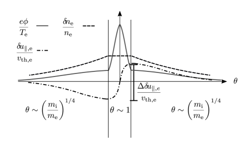
Figure 3: An illustration showing the nonadiabatic electron density $\delta\!n_{\rm{e}}$ and electron mean velocity $\delta\!u_{\|,\rm{e}}$ in the collisional, small-tail limit. The leading-order mode frequency is determined by ions in the $\theta\sim 1$ (outer) region, by solving equation (4) (with $s={\rm{i}}$) subject to quasineutrality, equation (118). The electron tails at $\theta\sim\left({m_{\rm{i}}}/{m_{\rm{e}}}\right)^{1/4}$ are obtained by solving the transport equations (85) and (86), with inner-region quasineutrality (84) and the boundary conditions (114) - (117). From the perspective of the $\theta\sim\left({m_{\rm{i}}}/{m_{\rm{e}}}\right)^{1/4}$ region, the electron density is a cusp, set up by the discontinuity in $\delta\!u_{\|,\rm{e}}$, $\Delta\delta\!u_{\|,\rm{e}}$.

Finally, we can describe the procedure for solving for the small-tail mode in the $\left(m_{\rm{e}}/m_{\rm{i}}\right)^{1/2}\rightarrow 0$ limit. To determine the frequency $\omega^{(0)}$ and the potential $\phi_{{\scriptsize\rm{outer}}}^{(0)}$, we solve the ion gyrokinetic equation (4) with $s={\rm{i}}$, closed by the quasineutrality relation (neglecting the electron nonadiabatic response)

$$\left(\frac{Z_{\rm{i}}T_{\rm{e}}}{T_{\rm{i}}}+1\right)\frac{e\phi_{{\scriptsize\rm{outer}}}^{(0)}}{T_{\rm{e}}}=\int J_{0{\rm{i}}}\frac{h_{{\rm{i}},{\scriptsize\rm{outer}}}^{(0)}}{n_{\rm{i}}}\;d^{3}\bm{v}.$$ (118)

With $\omega^{(0)}$ and $\phi_{{\scriptsize\rm{outer}}}^{(0)}$ determined, we can solve for the electron response using equations (85) and (86), with the inner-region quasineutrality equation (84). The causal link between the solution in the outer region and the inner region is provided by boundary matching conditions (114) - (117). An illustration demonstrating the matching in the collisional small-tail mode is given in figure 3.

5.4 Electron response in the outer region for large-tail modes.

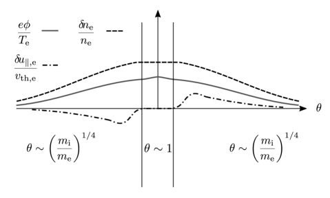
Figure 4: An illustration showing the nonadiabatic electron density $\delta\!n_{\rm{e}}$ and electron mean velocity $\delta\!u_{\|,\rm{e}}$ in the collisional, large-tail limit. At leading-order, the mode frequency is determined by the nonadiabatic electron response in the $\theta\sim\left({m_{\rm{i}}}/{m_{\rm{e}}}\right)^{1/4}$ (inner) region, by solving the transport equations (85) and (86), with inner-region quasineutrality (84), and the boundary conditions (114), (115), (119), and (120). The ion response to the leading-order frequency can be obtained by solving equation (4) (with $s={\rm{i}}$) subject to quasineutrality, equation (66). In the large-tail mode the leading-order flows are developed in the $\theta\sim\left({m_{\rm{i}}}/{m_{\rm{e}}}\right)^{1/4}$ region, and there is no leading-order electron density cusp near the boundary of the $\theta\sim 1$ region.

The large-tail ordering is the combination of the orderings (73) and (75). As a consequence, the equation for the leading-order electron response $H_{{\rm{e}},{\scriptsize\rm{outer}}}^{(0)}$ takes the form of equation (81). Following the same arguments as used in G, we can demonstrate that the solution to equation (81) is that the electron distribution is a perturbed Maxwellian with a fluctuating nonadiabatic density $\delta\!n^{(0)}_{\rm{e,outer}}$ and temperature $\delta\!T^{(0)}_{\rm{e,outer}}$, no flow, and no dependence on $\theta$, as required to match to the inner region. For the matching conditions on the leading-order distribution function, we require that the nonadiabatic density and temperature that define the electron distribution function are continuous across $\chi=0$ after equations (114) and (115), with $\delta\!n^{(0)}_{\rm{e,outer}}=\delta\!n^{(0)}_{\rm{e,inner}}(\chi=0)$ and $\delta\!T^{(0)}_{\rm{e,outer}}=\delta\!T^{(0)}_{\rm{e,inner}}(\chi=0)$.

For this class of modes, the frequency is determined by the eigenmode equations (85) and (86), with the inner-region quasineutrality equation (84) and the matching conditions (114) and (115). Because the eigenmode equations are second order differential equations in $\chi$, two further matching conditions are required. These conditions are that the electron flows $\overline{\delta\!u}_{\|}$ and $\overline{\delta\!q}_{\|}$ are continuous across $\chi=0$, i.e.,

$$\overline{\delta\!u}_{\|}(\chi=0^{+})=\overline{\delta\!u}_{\|}(\chi=0^{-}),$$ (119)

and

$$\overline{\delta\!q}_{\|}(\chi=0^{+})=\overline{\delta\!q}_{\|}(\chi=0^{-}).$$ (120)

Equations (119) and (120) can be derived by noting that the jump in the electron parallel flows across the outer region have a fixed size, given by the estimate (112). In a large tail mode, we have that

$$\frac{\delta\!u_{\|,\rm{e,inner}}}{v_{\rm{th,e}}}\sim\frac{\delta\!q_{\|,\rm{e,inner}}}{v_{\rm{th,e}}n_{\rm{e}}T_{\rm{e}}}\sim\left(\frac{m_{\rm{e}}}{m_{\rm{i}}}\right)^{1/4}\frac{e\phi_{{\scriptsize\rm{inner}}}}{T_{\rm{e}}}\sim\left(\frac{m_{\rm{e}}}{m_{\rm{i}}}\right)^{1/4}\frac{e\phi_{{\scriptsize\rm{outer}}}}{T_{\rm{e}}}\gg\left(\frac{m_{\rm{e}}}{m_{\rm{i}}}\right)^{1/2}\frac{e\phi_{{\scriptsize\rm{outer}}}}{T_{\rm{e}}}.$$ (121)

and hence the flows are continuous across the outer region to leading order. This result can be obtained explicitly by inspecting equations (116) and (117), with the ordering (121). An illustration of the structure of the collisional, large-tail mode is presented in figure 4.

Finally, we note that the nonadiabatic ion response has no role in determining the leading-order frequency $\omega^{(0)}$. Instead, the ions respond passively, serving only to self-consistently determine the electrostatic potential $\phi_{{\scriptsize\rm{outer}}}^{(0)}$ through the quasineutrality equation (66) (noting that here the velocity space dependence of $H^{(0)}_{{\rm{e}}}$ is given by equation (82)). Note that $\phi_{{\scriptsize\rm{outer}}}^{(0)}$ has not entered into the equations that determine the electron response in the large-tail mode.

6 Numerical results

In this section we present numerical results that support the analytical theory of the previous sections. We use the gyrokinetic code GS2 [28] to calculate the fastest-growing linear modes for parameters where we observe extended electron-driven tails in the ballooning eigenfunction.

We propose a novel method to test the analytical theory: for a given mode with extended tails, we scan in our expansion parameter $\left(m_{\rm{e}}/m_{\rm{i}}\right)^{1/2}$ and test the $\left(m_{\rm{e}}/m_{\rm{i}}\right)^{1/2}$ dependence of the eigenmodes and complex frequencies. When we perform the scan in $\left(m_{\rm{e}}/m_{\rm{i}}\right)^{1/2}$, we hold fixed $k_{y}\rho_{\rm{th,i}}$, so that we scan in the separation between the electron parallel streaming frequency $v_{\rm{th,e}}/qR_{0}$, and frequency of the drive $\omega_{\ast}\sim\omega$. We must also choose how to treat the collision frequency $\nu_{\rm{ee}}$: the normalised electron collision frequency $\nu_{\ast}=qR_{0}\nu_{\rm{ee}}/v_{\rm{th,e}}\epsilon^{3/2}$ is independent of $m_{{\rm{e}}}/m_{{\rm{i}}}$, and so in a physical mass scan we would vary $v_{\rm{th,e}}/qR_{0}$ and $\nu_{\rm{ee}}$, holding $\nu_{\ast}$ fixed. This physical mass scan is appropriate for the collisional limit (2). However, to test the “collisionless” limit (1), if $\nu_{\rm{ee}}$ is comparable to $\omega$, we need to enforce $\nu_{\rm{ee}}\sim\omega\sim\omega_{\ast}$ as $\left(m_{\rm{e}}/m_{\rm{i}}\right)^{1/2}\rightarrow 0$, meaning that we would vary $v_{\rm{th,e}}/qR_{0}$ but hold $a\nu_{\rm{ee}}/v_{\rm{th,i}}$ fixed.

In the analytical theory that we have developed here, geometrical factors from the magnetic geometry enter into the equations for the inner region only through the poloidal angle average $\left\langle{\cdot}\right\rangle^{\theta}$. Hence, modes that are driven by the electron response in the inner region are unlikely to be sensitive to the details of any given magnetic geometry. We therefore choose the simple Cyclone Base Case (CBC) [43] magnetic geometry to illustrate our theory: we study modes on a circular flux surface centred on the magnetic axis. To specify the magnetic geometry, we use the Miller equilibrium parameterisation [44]. We take the reference major radius $R_{0}=3.0a$, with the normalising length $a$ the half-diameter of the last closed flux surface. We examine microstability on the flux surface with minor radius $r=0.54a$. We take the safety factor to be $q=1.4$, the magnetic shear to be $\hat{s}=(q/r)dq/dr=0.8$, the plasma beta $\beta=0$, the Shafranov shift derivative $d\Delta/dr=0$, the elongation $\kappa=1.0$, the elongation derivative $d\kappa/dr=0.0$, the triangularity $\delta=0.0$, and the triangularity derivative $d\delta/dr=0.0$. The reference magnetic field is given by $B_{\scriptsize{\rm{ref}}}=I(\psi)/R_{\rm geo}$, i.e., toroidal magnetic field at the major radial position $R_{\rm geo}$. We take $R_{\rm geo}=R_{0}$. In section 2.2, we define local radial and binormal coordinates with units of length $x$ and $y$, respectively, and associated radial and binormal wavenumbers $k_{x}$ and $k_{y}$, respectively. We parameterise the radial wave number $k_{x}$ with $\theta_{0}=k_{x}/\hat{s}k_{y}$.

We consider a two-species plasma of ions and electrons, with $Z_{\rm{i}}=1$, equal temperatures $T_{\rm{i}}=T_{\rm{e}}$, and an equilibrium density gradient $a/L_{n}=0.733$, where the length scale $L_{n}=-dr/d\ln n_{\rm{e}}$. We take the equilibrium ion temperature gradient to be $a/L_{T_{\rm{i}}}=2.3$, where the equilibrium temperature gradient length scale of species $s$ is defined by $L_{T_{s}}=-dr/d\ln T_{s}$. These parameters have been chosen to be close to the CBC benchmark equilibrium profiles. In order to examine different instabilities with these CBC-like parameters, we vary $\theta_{0}$, the equilibrium electron temperature gradient length scale $L_{T_{\rm{e}}}$, and the normalised electron collisionality $\nu_{\ast}=qR_{0}\nu_{\rm{ee}}/v_{\rm{th,e}}\epsilon^{3/2}$, where $\epsilon=r/R_{0}=0.18$. In section 6.1, we take $\theta_{0}=1.57$ and a large electron temperature gradient $a/L_{T_{\rm{e}}}=3a/L_{T_{\rm{i}}}=6.9$, resulting in novel modes that conform to the large-tail mode ordering. In section 6.2, we take $\theta_{0}=0.1$ and equal electron and ion temperature gradients $a/L_{T_{\rm{e}}}=a/L_{T_{\rm{i}}}=2.3$. This allows us to consider a familiar ITG mode, where we demonstrate that the passing electron response satisfies the small-tail mode ordering. Finally, in section 6.3, we briefly discuss the transition between large-tail and small-tail modes as a function of $\theta_{0}$ in a scenario with $a/L_{T_{\rm{e}}}=3.45$ and $a/L_{T_{\rm{i}}}=2.3$.

For the simulations presented here, we use the following numerical resolutions: $n_{\theta}=33$ points per $2\pi$ element in the ballooning angle grid; $n_{\lambda}=27$ points in the pitch angle grid; and $n_{\varepsilon}=24$ points in the energy grid. The energy grid is constructed from a spectral speed grid [45], and the pitch angle grid is constructed from a Radau-Gauss grid for passing particles and an unevenly spaced grid for trapped particles. We give the number of $2\pi$ elements in the ballooning grid $n_{2\pi}$ and timestep size $\Delta t$ in each of the following subsections. The convergence of these resolutions was tested by doubling (or halving) each parameter.

6.1 Large tail modes

In this section we present numerical results that are consistent with the asymptotic theory of linear modes with large electron tails, summarised in sections 4.4 (the collisionless case) and 5.4 (the collisional case). In order to make the passing-electron-response-driven modes the fastest growing instability in the system, it is necessary to increase the electron drive with respect to the ion drive: we take $a/L_{T_{\rm{e}}}=3a/L_{T_{\rm{i}}}=6.9$, and we focus on modes at $k_{y}\rho_{\rm{th,i}}=0.5$ with $\theta_{0}=1.57$. We vary $\nu_{\ast}$ in order to see the effect of electron collisionality on the mode. The geometry and physical parameters of the simulations are otherwise as described at the start of this section. We use the full GS2 model collision operator [36, 37], including pitch angle scattering, energy diffusion, and momentum and energy conserving terms. For the parameters that we consider here, we find that the inclusion of pitch-angle scattering collisions is crucial for making the large-tail mode the fastest-growing instability.

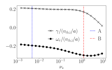
Figure 5: The growth rate $\gamma$ and frequency $\omega_{{\rm{r}}}$ for the large-tail mode with $\left({m_{\rm{i}}}/{m_{\rm{e}}}\right)^{1/2}=61$, $k_{y}\rho_{\rm{th,i}}=0.5$ and $\theta_{0}=1.57$, as a function of $\nu_{\ast}$. For $\nu_{\ast}<10^{-3}$ the large-tail mode is no longer the fastest-growing mode at this $(k_{y},\theta_{0})$. The vertical dashed lines A and B indicate the $\nu_{\ast}$ of the collisionless and collisional examples of large-tail modes that are predicted by the theory in sections 4.4 and 5.4, respectively.

In figure 5, we show the result of calculating the linear growth rate $\gamma$ and frequency $\omega_{{\rm{r}}}$ for the deuterium mass ratio $\left(m_{\rm{e}}/m_{\rm{i}}\right)^{1/2}\approx 1/61$ and a range of $\nu_{\ast}$. We vary the ion collision frequency $\nu_{\rm{ii}}$ consistently with $\nu_{\ast}$, i.e., $\nu_{\rm{ii}}=\epsilon^{3/2}\nu_{\ast}v_{\rm{th,i}}/\sqrt{2}qR_{0}$. We take $\Delta t=0.025a/v_{\rm{th,i}}$ and $n_{2\pi}=65$. For the range of $\nu_{\ast}$ shown in figure 5, we identify that the modes are large-tail modes, by a method which we now describe. We recall the cartoons given in figures 2 and 4. In a large-tail mode, the relative amplitude of the potential $\phi$ has the same size in the outer and inner regions as $\left(m_{\rm{e}}/m_{\rm{i}}\right)^{1/2}\rightarrow 0$, and the size of the passing part of the electron distribution function $H_{\rm{e}}$ in the outer and inner regions remains fixed as $\left(m_{\rm{e}}/m_{\rm{i}}\right)^{1/2}\rightarrow 0$. To demonstrate that the mode is a large-tail mode, we use a procedure with three steps. First, we perform a scan in the value of $\left(m_{\rm{e}}/m_{\rm{i}}\right)^{1/2}$. Second, we identify an integral measure of $H_{\rm{e}}$ and use it to demonstrate that $H_{{\rm{e}},{\scriptsize\rm{outer}}}\sim H_{{\rm{e}},{\scriptsize\rm{inner}}}$, independent of the value of $\left(m_{\rm{e}}/m_{\rm{i}}\right)^{1/2}$. Third, we plot $\phi$ normalised to the chosen integral measure of $H_{\rm{e}}$ and demonstrate that $\phi_{{\scriptsize\rm{outer}}}\sim\phi_{{\scriptsize\rm{inner}}}$, independent of the value of $\left(m_{\rm{e}}/m_{\rm{i}}\right)^{1/2}$. We can determine the scale of the inner region $\chi$ by using the scan in $\left(m_{\rm{e}}/m_{\rm{i}}\right)^{1/2}$ to determine $\alpha$ such that we can rescale $H_{\rm{e}}(\theta)\rightarrow H_{\rm{e}}(\theta\left({m_{\rm{e}}}/{m_{\rm{i}}}\right)^{\alpha})$ and so overlay the integral measure of $H_{\rm{e}}$ for the modes with different values of $\left(m_{\rm{e}}/m_{\rm{i}}\right)^{1/2}$. Collisionless modes are expected to have $\alpha=1/2$, whereas collisional modes are expected to have $\alpha=1/4$. To show how this procedure works in practice, we consider the clean examples of collisionless and collisional large-tail modes indicated by “A” and “B” on figure 5, respectively.

6.1.1 Case A – a collisionless large-tail mode.

In the first step in our procedure, we scan in the electron mass ratio from $m_{{\rm{e}}}/m_{{\rm{i}}}=5.4\times 10^{-4}$ to $5.4\times 10^{-5}$, whilst holding fixed $a\nu_{\rm{ee}}/v_{\rm{th,i}}=5.21\times 10^{-3}$. The value of $\nu_{\rm{ee}}$ is chosen so that $\nu_{\ast}=4.70\times 10^{-3}$ for the approximate deuterium mass ratio $(m_{{\rm D}}/m_{{\rm{e}}})^{1/2}=61$, and $\nu_{\rm{ii}}$ is set by $\nu_{\rm{ii}}/\nu_{\rm{ee}}=(m_{{\rm{e}}}/m_{{\rm D}})^{1/2}/\sqrt{2}$. In this example, we note that $\nu_{\ast}$ takes a similar value to $a\nu_{\rm{ee}}/v_{\rm{th,i}}$. This is a result of the large value of $qR_{0}/a\epsilon^{3/2}=55.0\sim(m_{{\rm D}}/m_{{\rm{e}}})^{1/2}$. To set $n_{2\pi}$ for different ion masses $m_{{\rm{i}}}$, we scale the number of $2\pi$ elements appropriately with mass ratio, i.e., $n_{2\pi}=65\sqrt{m_{{\rm{i}}}/m_{{\rm D}}}$. The timestep size is taken to be $\Delta t=0.025a/v_{\rm{th,i}}$.

In the second step of the procedure, we define a useful integral measure of the electron distribution function

$$j_{\|}=j^{+}_{\|}-j^{-}_{\|}$$ (122)

with

$$j^{\pm}_{\|}=-e\int^{\infty}_{0}\int^{1/B_{\rm max}}_{0}\frac{|v_{\|}|}{B}H_{\rm{e}}(\sigma=\pm 1)\;\frac{2\pi B\varepsilon}{m_{{\rm{e}}}^{2}|v_{\|}|}\;d\lambda\;d\varepsilon.$$ (123)

The field $j_{\|}$ has dimensions of current over magnetic field strength, and the quantities $j^{+}_{\|}$ and $j^{-}_{\|}$are the contributions from the forward going ($\sigma=1$) and backward going ($\sigma=-1$) particles, respectively. The prime usefulness of $j^{\pm}_{\|}$ stems from the fact that $H^{(0)}_{{\rm{e}}}$ is independent of the $2\pi$-periodic poloidal angle $\theta$ in the asymptotic theory, and hence, we expect that $j^{\pm}_{\|}$ are smoothly varying functions of ballooning angle, with minimal geometric $2\pi$-periodic oscillation. We can use $j^{+}_{\|}$ as a proxy to visualise the distribution of forward-going particles. In figure 6, we plot $|j^{+}_{\|}|$, normalised to its maximum value, for different values of $\left({m_{\rm{i}}}/{m_{\rm{e}}}\right)^{1/2}$. Figure 6 shows that $j^{+}_{\|}$ is self-similar for modes with different $\left(m_{\rm{e}}/m_{\rm{i}}\right)^{1/2}$, provided that the ballooning angle $\theta$ is rescaled to $\theta/\left({m_{\rm{i}}}/{m_{\rm{e}}}\right)^{1/2}$. This confirms that $H_{{\rm{e}},{\scriptsize\rm{outer}}}\sim H_{{\rm{e}},{\scriptsize\rm{inner}}}$, and that $\chi\sim\left({m_{\rm{i}}}/{m_{\rm{e}}}\right)^{1/2}$.

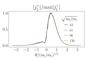
Figure 6: The field $j^{+}_{\|}$, calculated for different mass ratios holding fixed $a\nu_{\rm{ee}}/v_{\rm{th,i}}=5.21\times 10^{-3}$ ($\nu_{\ast}=4.70\times 10^{-3}$ for $\left({m_{\rm{i}}}/{m_{\rm{e}}}\right)^{1/2}=61$ – case A of figure 5). Note that the curves overlay on the $\theta/\left({m_{\rm{i}}}/{m_{\rm{e}}}\right)^{1/2}$ axis.

Finally, in the last step of the procedure, we visualise the electrostatic potential in figure 7. We normalise the potential to the maximum value of $|j^{+}_{\|}|$, and give the result $|\phi|/{\rm max}|j^{+}_{\|}|$ in the units of $\phi^{{\rm{ref}}}/j_{\|}^{{\rm{ref}}}$, where $\phi^{{\rm{ref}}}=T_{\rm{e}}/e$ and $j_{\|}^{{\rm{ref}}}=en_{\rm{e}}v_{\rm{th,e}}/B_{{\rm{ref}}}$. In figure 7, we can see that $\phi$ has an envelope on the scale of $\theta\sim\left({m_{\rm{i}}}/{m_{\rm{e}}}\right)^{1/2}$, and an irreducible geometric structure on the scale of $\theta\sim 2\pi$. The envelope of $|\phi|$ overlays well in figure 7, confirming that $\phi_{{\scriptsize\rm{outer}}}\sim\phi_{{\scriptsize\rm{inner}}}$ and, hence, that the mode is a large-tail mode. The geometric $2\pi$-oscillations in $\phi$ appear because of the geometric poloidal angle dependence in the Jacobian $2\pi B\varepsilon/m_{{\rm{e}}}^{2}|v_{\|}|$ of the velocity integral, equation (140); because of the inclusion of trapped particles in the velocity integral; and because of the appearance of the Bessel function $J^{(0)}_{0{\rm{e}}}$ and phase $\exp{\left[{\rm{i}}\lambda_{{\rm{e}}}\chi\right]}$ in the quasineutrality relation in the large-$\theta$ region, equation (70).

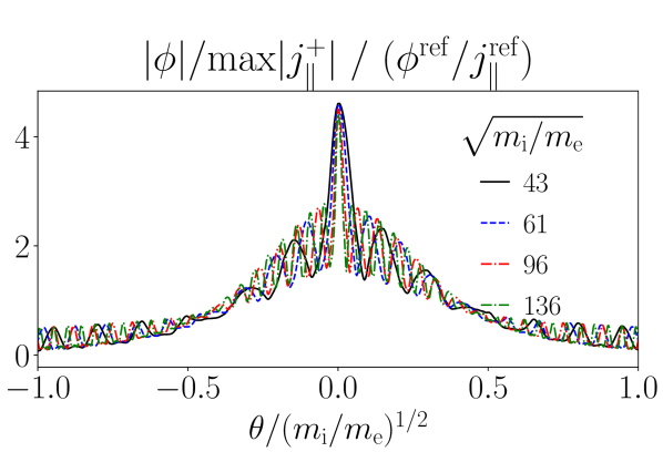
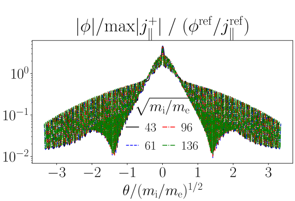
Figure 7: Two views of the electrostatic potential $\phi$, for different mass ratios holding fixed $a\nu_{\rm{ee}}/v_{\rm{th,i}}=5.21\times 10^{-3}$ (corresponding to $\nu_{\ast}=4.70\times 10^{-3}$ when $\left({m_{\rm{i}}}/{m_{\rm{e}}}\right)^{1/2}=61$, case A of figure 5). The potential is plotted against the scaled ballooning angle $\theta/\left({m_{\rm{i}}}/{m_{\rm{e}}}\right)^{1/2}$, and normalised to the maximum value of $j^{+}_{\|}$ (see equation (123) and figure 6). The fact that the curves overlay on the $\theta/\left({m_{\rm{i}}}/{m_{\rm{e}}}\right)^{1/2}$ axis confirms that the mode is a collisionless large-tail mode. Note the geometric $2\pi$-periodic oscillation in $\phi$ due to geometric factors in the velocity integral over the electron distribution function (cf. equation (70)). The dimensions are $\phi^{{\rm{ref}}}=T_{\rm{e}}/e$ and $j_{\|}^{{\rm{ref}}}=en_{\rm{e}}v_{\rm{th,e}}/B_{\scriptsize{\rm{ref}}}$.

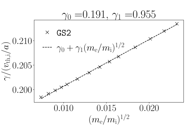
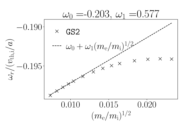
Figure 8: Plots of the growth rate $\gamma$ (left) and real frequency $\omega_{{\rm{r}}}$ (right) as a function of $\left(m_{\rm{e}}/m_{\rm{i}}\right)^{1/2}$, for fixed $a\nu_{\rm{ee}}/v_{\rm{th,i}}=5.21\times 10^{-3}$ (corresponding to case A of figure 5 when $\left({m_{\rm{i}}}/{m_{\rm{e}}}\right)^{1/2}=61$ and $\nu_{\ast}=4.70\times 10^{-3}$). We give a linear fit to demonstrate that the dependence of $\gamma$ and $\omega_{{\rm{r}}}$ on $\left(m_{\rm{e}}/m_{\rm{i}}\right)^{1/2}$ is consistent with a $\left(m_{\rm{e}}/m_{\rm{i}}\right)^{1/2}$ expansion of the form given by equation (30).

From the asymptotic theory in section 4, we would expect to see that the growth rate had a leading order piece $\gamma^{(0)}$, and an $\Or\left(\left(m_{\rm{e}}/m_{\rm{i}}\right)^{1/2}\right)$ small correction $\gamma^{(1)}$. In figure 8, we plot $\gamma$ (figure 8, left) and $\omega_{{\rm{r}}}$ (figure 8, right) as a function of $\left(m_{\rm{e}}/m_{\rm{i}}\right)^{1/2}$. The linear fits are provided to show that the changes with $\left(m_{\rm{e}}/m_{\rm{i}}\right)^{1/2}$ in $\gamma$ and $\omega_{{\rm{r}}}$ are consistent with an expansion in $\left(m_{\rm{e}}/m_{\rm{i}}\right)^{1/2}$: the fit parameters are of order unity, and the overall variation in $\gamma$ and $\omega_{{\rm{r}}}$ is small. We note that the linear fit is particularly good for $\gamma$ for the whole range of $\left(m_{\rm{e}}/m_{\rm{i}}\right)^{1/2}$. In the case of $\omega_{{\rm{r}}}$, we see a linear trend arise only at small $\left(m_{\rm{e}}/m_{\rm{i}}\right)^{1/2}$. In general, we would expect to recover a linear trend for sufficiently small $\left(m_{\rm{e}}/m_{\rm{i}}\right)^{1/2}$. We note that, because $\nu_{\rm{ee}}/\omega\ll 1$, the qualitative results of figures 6-8 can be reproduced by a scan holding fixed $\nu_{\ast}$ rather than $a\nu_{\rm{ee}}/v_{\rm{th,i}}$, providing that $\nu_{\rm{ee}}/\omega$ does not approach values of order unity.

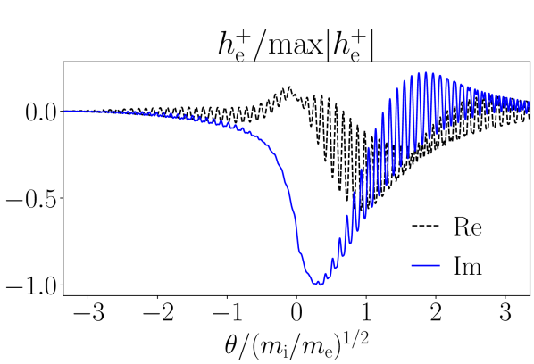
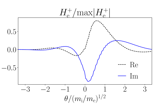
Figure 9: The distribution function for forward going particles, for the mode with $\left({m_{\rm{i}}}/{m_{\rm{e}}}\right)^{1/2}=61$ in figure 6, for $\varepsilon/T_{\rm{e}}=0.79$ and $\lambda B_{{\rm{ref}}}=0.22$. Left, we plot $h_{{\rm{e}}}$ for forward going particles. Note the rapid oscillation in $\theta$ for $\theta\gg 1$. Right, we plot $H_{\rm{e}}$ for forward going particles. Note the smoothness of $H_{\rm{e}}$ compared to $h_{{\rm{e}}}$ for $\theta\gg 1$.

Finally, we comment on the use of the modified distribution function $H_{\rm{e}}$ in place of the usual nonadiabatic response $h_{{\rm{e}}}$ in the asymptotic theory. In figure 9, we plot the distribution functions $h_{{\rm{e}}}$ and $H_{\rm{e}}$, as a function of $\theta$, for the velocity space element $\varepsilon/T_{\rm{e}}=0.79$, $\lambda B_{{\rm{ref}}}=0.22$ and $\sigma=1$. We show the distribution functions for the $\left({m_{\rm{i}}}/{m_{\rm{e}}}\right)^{1/2}=61$ mode featured in figure 6. We observe that the distribution function $h_{{\rm{e}}}$ shows large $2\pi$-scale oscillations in phase, whereas $H_{\rm{e}}$ is a smoothly varying function. In general, $H_{\rm{e}}$ appears to be a smoother variable than $h_{{\rm{e}}}$ for the parts of the electron distribution function where $v_{\|}\sim v_{\rm{th,e}}\gg v_{\rm{th,i}}$. These observations justify the choice to use the modified distribution function $H_{\rm{e}}$ in the asymptotic theory.

6.1.2 Case B – a collisional large-tail mode.

We now consider an example of a collisional large-tail mode. We must demonstrate that $H_{{\rm{e}},{\scriptsize\rm{outer}}}\sim H_{{\rm{e}},{\scriptsize\rm{inner}}}$ and $\phi_{{\scriptsize\rm{outer}}}\sim\phi_{{\scriptsize\rm{inner}}}$ as $\left({m_{\rm{e}}}/{m_{\rm{i}}}\right)^{1/4}\rightarrow 0$, and show that the envelope of the eigenmode scales like $\chi\sim\left({m_{\rm{i}}}/{m_{\rm{e}}}\right)^{1/4}$. The physics parameters are identical to those of the collisionless large-tail mode described in section 6.1.1, except that the electron collisionality is increased to $\nu_{\ast}=1.22$. We scan in the electron mass ratio from $m_{{\rm{e}}}/m_{{\rm{i}}}=5.4\times 10^{-4}$ to $5.0\times 10^{-6}$ while holding $\nu_{\ast}$ fixed. We take $\nu_{\rm{ii}}=\epsilon^{3/2}\nu_{\ast}v_{\rm{th,i}}/\sqrt{2}qR_{0}$. Anticipating that the scale of the ballooning envelope should go with $\left({m_{\rm{i}}}/{m_{\rm{e}}}\right)^{1/4}$ in the collisional limit, in this case we take $n_{2\pi}=39(m_{{\rm{i}}}/m_{{\rm D}})^{1/4}$. Perhaps due to the larger collision frequency, we find that convergence is reached only with relatively small timesteps for the largest $\left({m_{\rm{i}}}/{m_{\rm{e}}}\right)^{1/4}$ considered in the scan. In the simulations presented here $\Delta t=0.00625a/v_{\rm{th,i}}$. Obtaining convergence in $\Delta t$ is more challenging for smaller $\left({m_{\rm{e}}}/{m_{\rm{i}}}\right)^{1/4}$.

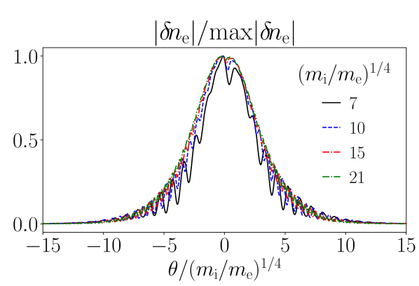
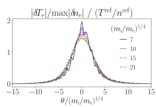
Figure 10: (left) The electron nonadiabatic density $\delta\!n_{\rm{e}}$, calculated for $\nu_{\ast}=1.22$ (case B of figure 5) for different mass ratios. The density is normalised to its maximum value, and plotted against the scaled ballooning angle $\theta/\left({m_{\rm{i}}}/{m_{\rm{e}}}\right)^{1/4}$. (right) The electron temperature, normalised to the maximum value of the electron nonadiabatic density. Here $n^{\scriptsize{\rm{ref}}}=n_{\rm{e}}$, $T^{{\rm{ref}}}=T_{\rm{e}}$.

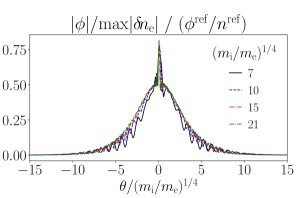
Figure 11: The electrostatic $\phi$, calculated for $\nu_{\ast}=1.22$ (case B of figure 5) for different mass ratios. The potential is normalised to the maximum value of $\delta\!n_{\rm{e}}$, ${\rm{max}}|\delta\!n_{\rm{e}}|$. The good agreement for the rescaled potential normalised to ${\rm{max}}|\delta\!n_{\rm{e}}|$ suggests that this mode can be regarded as a collisional large-tail mode. Here $\phi^{{\rm{ref}}}=T_{\rm{e}}/e$ and $n^{\scriptsize{\rm{ref}}}=n_{\rm{e}}$.

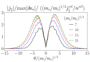
Figure 12: The current-like field $j_{\|}$, defined in equation (122), normalised to the maximum value of $\delta\!n_{\rm{e}}$, for $\nu_{\ast}=1.22$ (case B of figure 5). Note that $j_{\|}$ is a $\left({m_{\rm{e}}}/{m_{\rm{i}}}\right)^{1/4}$ small quantity. If the numerics perfectly reproduced the asymptotic theory of section 5, the plotted curves would overlay. The $\left({m_{\rm{i}}}/{m_{\rm{e}}}\right)^{1/4}$ rescaling produces better agreement than a $\left({m_{\rm{i}}}/{m_{\rm{e}}}\right)^{1/2}$ rescaling, and we note that the curves appear to be converging for the largest $\left({m_{\rm{i}}}/{m_{\rm{e}}}\right)^{1/4}$. Here, $j_{\|}^{{\rm{ref}}}=en_{\rm{e}}v_{\rm{th,e}}/B_{\scriptsize{\rm{ref}}}$ and $n^{\scriptsize{\rm{ref}}}=n_{\rm{e}}$.

In the collisional ordering, the asymptotic theory of large-tail modes in section 5 indicates that there are three leading-order quantities that are free from geometric $2\pi$ poloidal angle oscillations at large $\theta$: the electron nonadiabatic density $\delta\!n_{\rm{e}}$, the electron temperature $\delta\!T_{\rm{e}}$, and the electrostatic potential $\phi$. The electron nonadiabatic density and temperature are plotted in figure 10, with the ballooning angle $\theta$ rescaled by $\left({m_{\rm{i}}}/{m_{\rm{e}}}\right)^{1/4}$. We observe good agreement for different $\left({m_{\rm{i}}}/{m_{\rm{e}}}\right)^{1/4}$ in the mass ratio scan. In figure 11, we plot the electrostatic potential $\phi$, normalised to the maximum value of $\delta\!n_{\rm{e}}$. Figure 11 shows good agreement for different $\left({m_{\rm{i}}}/{m_{\rm{e}}}\right)^{1/4}$. Together, figures 10 and 11 demonstrate that the mode featured is a collisional large-tail mode.

In the asymptotic theory of the collisional large-tail mode, the parallel-to-the-field flows play an important diffusive role, despite being small by $\left({m_{\rm{e}}}/{m_{\rm{i}}}\right)^{1/4}$. In figure 12, we plot the current-like field $j_{\|}$, defined in equation (122), with the ballooning angle $\theta$ rescaled by $\left({m_{\rm{i}}}/{m_{\rm{e}}}\right)^{1/4}$, and the amplitude rescaled by $\left({m_{\rm{e}}}/{m_{\rm{i}}}\right)^{1/4}$. Although the curves do not overlay perfectly in the $\left({m_{\rm{i}}}/{m_{\rm{e}}}\right)^{1/4}$ ballooning angle rescaling, the curves appear to be converging for the largest $\left({m_{\rm{i}}}/{m_{\rm{e}}}\right)^{1/4}$ in the scan. We note that the $\left({m_{\rm{i}}}/{m_{\rm{e}}}\right)^{1/4}$ ballooning angle rescaling shown in figure 12 gives better agreement than a $\left({m_{\rm{i}}}/{m_{\rm{e}}}\right)^{1/2}$ ballooning angle rescaling.

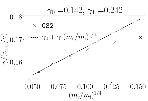
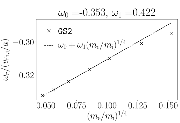
Figure 13: Plots of the growth rate $\gamma$ (left) and real frequency $\omega_{{\rm{r}}}$ (right) as a function of $\left({m_{\rm{e}}}/{m_{\rm{i}}}\right)^{1/4}$, for $\nu_{\ast}=1.22$ (case B of figure 5). We give a linear fit to illustrate the dependence of $\gamma$ and $\omega_{{\rm{r}}}$ on $\left({m_{\rm{e}}}/{m_{\rm{i}}}\right)^{1/4}$.

The asymptotic expansion for the collisional large-tail mode is carried out in powers of $\left({m_{\rm{e}}}/{m_{\rm{i}}}\right)^{1/4}$. In consequence, we would expect that $\gamma$ and $\omega_{{\rm{r}}}$ would have leading order components $\gamma^{(0)}$ and $\omega^{(0)}_{{\rm{r}}}$, respectively, that are independent of mass ratio, and sub-leading components $\gamma^{(1/2)}$ and $\omega^{(1/2)}_{{\rm{r}}}$, respectively, that scale linearly with $\left({m_{\rm{e}}}/{m_{\rm{i}}}\right)^{1/4}$. In figure 13 we plot $\gamma$ and $\omega_{{\rm{r}}}$ versus $\left({m_{\rm{e}}}/{m_{\rm{i}}}\right)^{1/4}$, with linear fits given to indicate the order of magnitude of the variation with $\left({m_{\rm{e}}}/{m_{\rm{i}}}\right)^{1/4}$. The fit coefficients are of order unity consistent with a $\left({m_{\rm{e}}}/{m_{\rm{i}}}\right)^{1/4}$ expansion. We note that a nonlinear trend is observed in $\gamma$ for the smallest $\left({m_{\rm{e}}}/{m_{\rm{i}}}\right)^{1/4}$. This may be a result of numerical difficulties, in light of the very small $\Delta t$ required to converge the smallest $\left({m_{\rm{e}}}/{m_{\rm{i}}}\right)^{1/4}$ points in figure 13.

6.2 Small tail modes

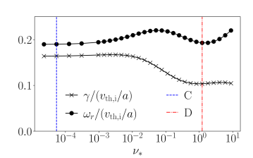
Figure 14: The growth rate $\gamma$ and real frequency $\omega_{{\rm{r}}}$ of the (small-tail), ITG mode with $k_{y}\rho_{\rm{th,i}}=0.5$, $\theta_{0}=0.1$, and $\left({m_{\rm{i}}}/{m_{\rm{e}}}\right)^{1/2}=61$, as a function of normalised electron collisionality $\nu_{\ast}$. Note that $\gamma$ and $\omega_{{\rm{r}}}$ experience $\Or\left(1\right)$ changes for $\nu_{\ast}\gtrsim 10^{-2}$. We explain this feature in figure 15. The vertical dashed lines C and D indicate the $\nu_{\ast}$ of the collisionless and collisional examples of the small-tail mode that are predicted by the theory in sections 4.3 and 5.3, respectively.

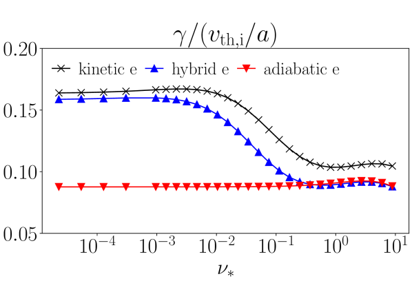
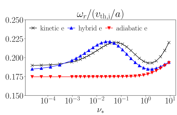
Figure 15: The ITG mode growth rate $\gamma$ (left) and real frequency $\omega_{{\rm{r}}}$ (right), calculated for the physical parameters given in figure 14, for three different electron response models: the fully kinetic electron response (black crosses); a hybrid electron response, where the passing electrons are forced to respond adiabatically, but trapped electrons respond kinetically (blue upward triangles); and a fully adiabatic electron response (red downward triangles). Note that the fully kinetic electron response results in a similar growth rate to the case with a hybrid electron response – this implies that trapped electrons are responsible for the $\Or\left(1\right)$ variation in $\gamma$ and $\omega_{{\rm{r}}}$.

In this section we verify the mass ratio scalings for collisionless small-tail modes, described in section 4.3, and collisional small-tail modes, described in section 5.3. We focus on the example of the ITG mode. We perform simulations using the magnetic geometry described at the start of section 6. We we take the temperature and density scale lengths to be $a/L_{T_{\rm{i}}}=a/L_{T_{\rm{e}}}=2.3$ and $a/L_{n}=0.733$, respectively. We examine the mode with $k_{y}\rho_{\rm{th,i}}=0.5$ and $\theta_{0}=0.1$.

In figure 14, we plot the growth rate $\gamma$ and real frequency $\omega_{{\rm{r}}}$ as a function of $\nu_{\ast}$, for $\left({m_{\rm{i}}}/{m_{\rm{e}}}\right)^{1/2}=61$. We take $\Delta t=0.025a/v_{\rm{th,i}}$ and $n_{2\pi}=65$. We set the ion collision frequency consistent with $\nu_{\ast}$, i.e., $\nu_{\rm{ii}}=\epsilon^{3/2}\nu_{\ast}v_{\rm{th,i}}/\sqrt{2}qR_{0}$. By scanning in $\left(m_{\rm{e}}/m_{\rm{i}}\right)^{1/2}$, we identify that the modes in figure 14 are small-tail modes by verifying that the $\theta\gg 1$ part of the eigenmode $e\phi_{{\scriptsize\rm{inner}}}/T_{\rm{e}}$ is bounded by the estimates $\left(m_{\rm{e}}/m_{\rm{i}}\right)^{1/2}e\phi_{{\scriptsize\rm{outer}}}/T_{\rm{e}}$ (the collisionless case, where $\nu_{\rm{ee}}\lesssim\omega$ and we hold $a\nu_{\rm{ee}}/v_{\rm{th,i}}$ fixed) and $\left({m_{\rm{e}}}/{m_{\rm{i}}}\right)^{1/4}e\phi_{{\scriptsize\rm{outer}}}/T_{\rm{e}}$ (the collisional case, where $\nu_{\rm{ee}}\gg\omega$, $\nu_{\ast}\sim 1$ and we hold $\nu_{\ast}$ fixed). The vertical dashed lines indicate the $\nu_{\ast}$ of the clean examples of the collisionless and collisional small-tail modes that we describe in detail in the following sections. Figure 14 shows that $\gamma$ and $\omega_{{\rm{r}}}$ depend on $\nu_{\ast}$ for $\nu_{\ast}\gtrsim 10^{-2}$. In figure 15, we demonstrate that this $\nu_{\ast}$ dependence arises from the trapped electron response. We compare $\gamma$ and $\omega_{{\rm{r}}}$ of the ITG mode calculated using three different electron responses (cf. [13, 33, 46]): the fully kinetic electron response (black crosses), a hybrid electron response with kinetic trapped electrons and adiabatic passing electrons (blue triangles), and adiabatic electrons (red triangles). By comparing the hybrid electron case to the adiabatic electron case, we see that for very small $\nu_{\ast}$, trapped electrons are decoupled from passing electrons and provide an $\Or\left(1\right)$ modification to the growth rate. When $\nu_{\ast}$ become sufficiently large, the effect of collisions is to detrap the trapped electrons so that the electron response is essentially adiabatic. The difference between the cases with the fully kinetic electron response and the hybrid electron response shows that passing electrons make a small modification to $\gamma$ and $\omega_{{\rm{r}}}$, consistent with the asymptotic theory. We note that simulations with adiabatic passing electrons can be converged with small $n_{2\pi}$: for the simulations presented here we take $n_{2\pi}=9$.

6.2.1 Case C – a collisionless small-tail mode.

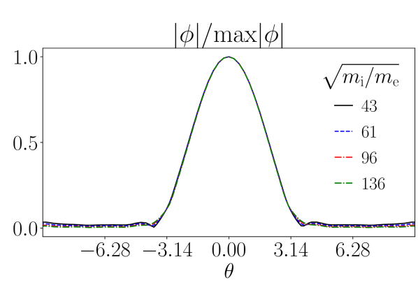
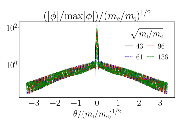
Figure 16: Two views of the electrostatic potential $\phi$, calculated for different mass ratios with fixed $a\nu_{\rm{ee}}/v_{\rm{th,i}}=5.98\times 10^{-5}$, corresponding to case C of figure 14 when $\left({m_{\rm{i}}}/{m_{\rm{e}}}\right)^{1/2}=61$, and hence, $\nu_{\ast}=5.40\times 10^{-5}$. (left) The potential $\phi$ is plotted against the unscaled ballooning angle $\theta$, and normalised to its maximum value. The fact that the curves overlay for $\theta\sim 1$ indicates that the potential eigenmode is independent of $\left(m_{\rm{e}}/m_{\rm{i}}\right)^{1/2}$ to leading order. (right) The potential is plotted against the scaled ballooning angle $\theta/\left({m_{\rm{i}}}/{m_{\rm{e}}}\right)^{1/2}$, and normalised by a factor of $\left(m_{\rm{e}}/m_{\rm{i}}\right)^{1/2}{\rm max}|\phi|$. The fact that the curves overlap in the region $\theta\sim\left({m_{\rm{i}}}/{m_{\rm{e}}}\right)^{1/2}$ indicates that the mode is a small-tail mode, satisfying the ordering (72).

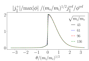
Figure 17: The field $j^{+}_{\|}$, calculated for different mass ratios and fixed $a\nu_{\rm{ee}}/v_{\rm{th,i}}=5.98\times 10^{-5}$, corresponding to $\nu_{\ast}=5.40\times 10^{-5}$ for $\left({m_{\rm{i}}}/{m_{\rm{e}}}\right)^{1/2}=61$ (case C of figure 14). The fact that the curves overlay on the $\theta/\left({m_{\rm{i}}}/{m_{\rm{e}}}\right)^{1/2}$ axis confirms that the mode is a collisionless small-tail mode, satisfying the ordering (71).

We consider the ITG mode from figure 14 with $\nu_{\ast}=5.40\times 10^{-5}$. We scan in $m_{{\rm{e}}}/m_{{\rm{i}}}=5.4\times 10^{-4}$ to $5.4\times 10^{-5}$, whilst holding fixed $a\nu_{\rm{ee}}/v_{\rm{th,i}}=5.98\times 10^{-5}$. The value of $\nu_{\rm{ee}}$ is chosen so that $\nu_{\ast}=5.40\times 10^{-5}$ for $\left({m_{\rm{i}}}/{m_{\rm{e}}}\right)^{1/2}=(m_{{\rm D}}/m_{{\rm{e}}})^{1/2}$, and we take $\nu_{\rm{ii}}/\nu_{\rm{ee}}=(m_{{\rm{e}}}/m_{{\rm D}})^{1/2}/\sqrt{2}$. To identify a mode as a collisionless small-tail mode, we must demonstrate several properties. First, that there is a $\theta\sim 1$ region where $e\phi/T_{\rm{e}}$ is independent of $\left(m_{\rm{e}}/m_{\rm{i}}\right)^{1/2}$ at leading order. Second, that the potential in the $\theta\gg 1$ region has an amplitude given by estimate (72), and an envelope $\theta\sim\left({m_{\rm{i}}}/{m_{\rm{e}}}\right)^{1/2}$. Third, that the electron distribution function has a size given by estimate (71), and an envelope with scale $\theta\sim\left({m_{\rm{i}}}/{m_{\rm{e}}}\right)^{1/2}$. In figure 16, we demonstrate that the first and second properties are satisfied. In figure 17, we use $j^{+}_{\|}$ as a measure of $H_{\rm{e}}$ to demonstrate that the third property is satisfied. In these simulations, we take $\Delta t=0.025a/v_{\rm{th,i}}$ and $n_{2\pi}=65\sqrt{m_{{\rm{i}}}/m_{{\rm D}}}$.

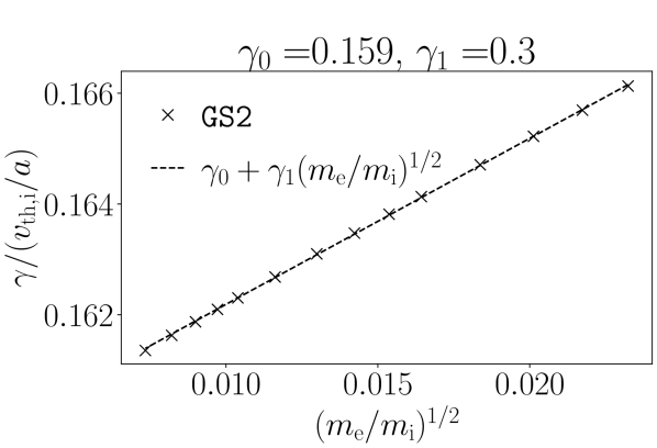
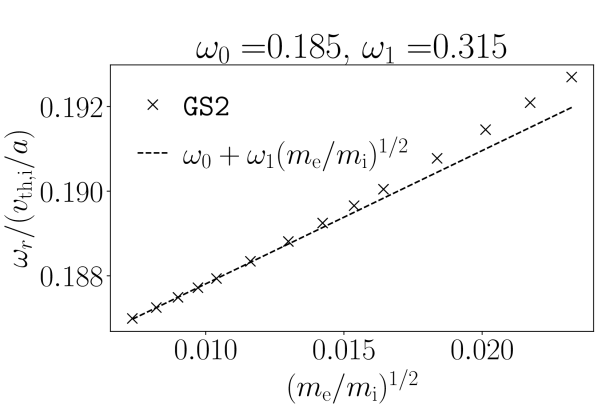
Figure 18: Plots of the growth rate $\gamma$ (left) and real frequency $\omega_{{\rm{r}}}$ (right) as a function of $\left(m_{\rm{e}}/m_{\rm{i}}\right)^{1/2}$, for the mode featured in figures 16 and 17. We give a linear fit to demonstrate that the dependence of $\gamma$ and $\omega_{{\rm{r}}}$ on $\left({m_{\rm{e}}}/{m_{\rm{i}}}\right)^{1/2}$ is consistent with a $\left({m_{\rm{e}}}/{m_{\rm{i}}}\right)^{1/2}$ expansion.

Finally, we discuss the $\left(m_{\rm{e}}/m_{\rm{i}}\right)^{1/2}$ dependence of the growth rate $\gamma$ and real frequency $\omega_{{\rm{r}}}$ in the collisionless example small-tail mode featured in figures 16 and 17. The growth rate and frequency are plotted in figure 18. As the asymptotic expansion is carried out in $\left(m_{\rm{e}}/m_{\rm{i}}\right)^{1/2}$, we expect to see a linear dependence in $\left(m_{\rm{e}}/m_{\rm{i}}\right)^{1/2}$. This is observed for a wide range of $\left(m_{\rm{e}}/m_{\rm{i}}\right)^{1/2}$ in $\gamma$, but for a smaller range of $\left(m_{\rm{e}}/m_{\rm{i}}\right)^{1/2}$ for $\omega_{{\rm{r}}}$. We note that the fit coefficients are of order unity, confirming that the dependence of $\gamma$ and $\omega_{{\rm{r}}}$ on $\left(m_{\rm{e}}/m_{\rm{i}}\right)^{1/2}$ is consistent with the $\left(m_{\rm{e}}/m_{\rm{i}}\right)^{1/2}$ expansion.

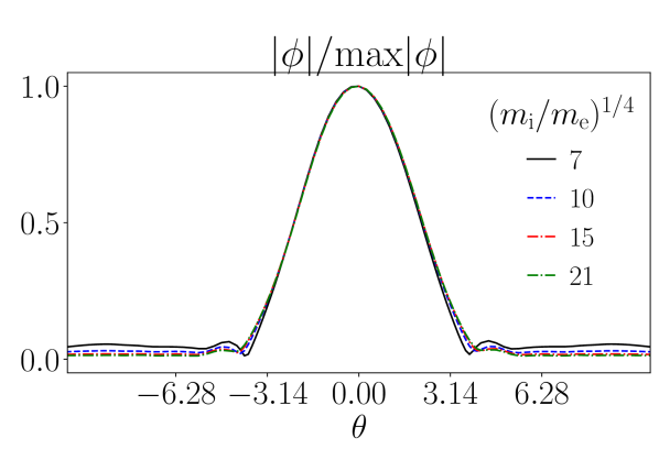
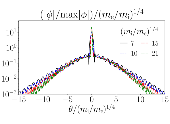
Figure 19: Two views of the electrostatic potential $\phi$, calculated for $\nu_{\ast}=1.22$ (case D of figure 14) for different mass ratios. (left) The potential $\phi$ is plotted against the unscaled ballooning angle, and normalised to its maximum value. That the curves overlay in the $\theta\sim 1$ region indicates that the mode is a small-tail mode. (right) The potential $\phi$ is plotted against the scaled ballooning angle $\theta/\left({m_{\rm{i}}}/{m_{\rm{e}}}\right)^{1/4}$, and normalised to its maximum value, divided by $\left({m_{\rm{e}}}/{m_{\rm{i}}}\right)^{1/4}$. That the curves overlay for $\theta\sim\left({m_{\rm{i}}}/{m_{\rm{e}}}\right)^{1/4}$ indicates that we have correctly identified the scaling (113) for the size of the electron response, and the size of the mode envelope.

6.2.2 Case D – a collisional small-tail mode.

In the collisional limit, the electron response of a small-tail mode is characterised by a jump in the electron flows across the $\theta\sim 1$ region. This results in the scalings (113) for the electrostatic potential, electron density, and electron temperature in the $\theta\gg 1$ region. As in the large-tail collisional mode, the size of the envelope of the mode is expected to be of scale $\theta\sim\left({m_{\rm{i}}}/{m_{\rm{e}}}\right)^{1/4}$. To test these scalings, we examine an ITG mode with normalised electron collision frequency $\nu_{\ast}=1.22$ (case D of figure 14). We scan in $m_{{\rm{e}}}/m_{{\rm{i}}}$ from $5.4\times 10^{-4}$ to $5.0\times 10^{-6}$ while holding $\nu_{\ast}$ fixed. We plot the electrostatic potential $\phi$ in figure 19. We note that $\phi$ has no mass dependence for $\theta\sim 1$, and that $\phi$ has the mass scaling given by the estimate (113) for $\theta\sim\left({m_{\rm{i}}}/{m_{\rm{e}}}\right)^{1/4}$. This confirms that the mode is a collisional, small-tail mode. In the simulations, we take $\Delta t=0.025a/v_{\rm{th,i}}$ and $n_{2\pi}=39(m_{{\rm{i}}}/m_{{\rm D}})^{1/4}$.

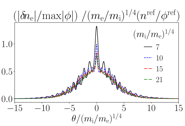
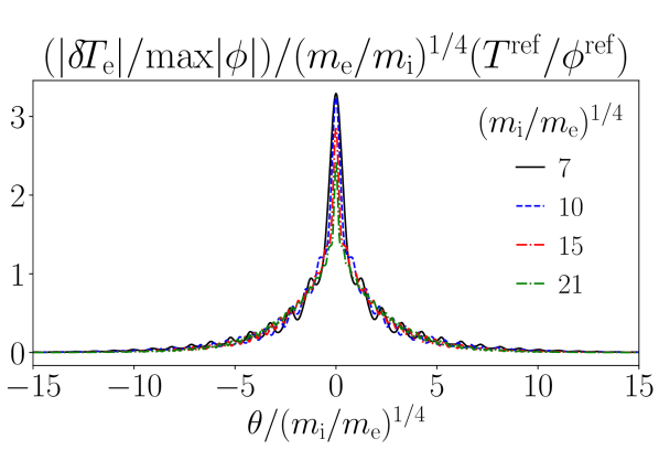
Figure 20: (left) The electron nonadiabatic density $\delta\!n_{\rm{e}}$, and (right) the electron temperature $\delta\!T_{\rm{e}}$, calculated for $\nu_{\ast}=1.22$ (case D of figure 14) for different mass ratios.

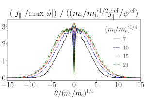
Figure 21: The field $j_{\|}$, calculated for $\nu_{\ast}=1.22$ (case D of figure 14) for different mass ratios. Whilst the curves do not overlay perfectly, we note that the curves appear to be converging for the largest $\left({m_{\rm{i}}}/{m_{\rm{e}}}\right)^{1/4}$ in the scan.

To illustrate the electron response further, we plot the nonadiabatic electron density $\delta\!n_{\rm{e}}$ and electron temperature $\delta\!T_{\rm{e}}$ in figure 20. The scaling (113) is confirmed by the fact that the curves overlay with the mass scaling $\left({m_{\rm{e}}}/{m_{\rm{i}}}\right)^{1/4}$ in the amplitude, and the mass scaling $\left({m_{\rm{i}}}/{m_{\rm{e}}}\right)^{1/4}$ in the ballooning angle. In figure 21, we plot the field $j_{\|}$, normalised to the maximum value of $|\phi|$. Consistent with the identification of the mode as a collisional small-tail mode, the envelope of $j_{\|}$ appears to scale like $\theta\sim\left({m_{\rm{i}}}/{m_{\rm{e}}}\right)^{1/4}$, and the amplitude is small by $\left(m_{\rm{e}}/m_{\rm{i}}\right)^{1/2}$. Although the envelope rescaling is not perfect in figure 21, the curves appear to be converging for the largest $\left({m_{\rm{i}}}/{m_{\rm{e}}}\right)^{1/4}$ in the scan. We note that the $\left({m_{\rm{i}}}/{m_{\rm{e}}}\right)^{1/4}$ rescaling is better than a $\left({m_{\rm{i}}}/{m_{\rm{e}}}\right)^{1/2}$ rescaling. This figure completes the demonstration of the physical picture for the collisional small-tail mode: the ions generate an electrostatic potential at $\theta\sim 1$, the electrons respond with a $\left(m_{\rm{e}}/m_{\rm{i}}\right)^{1/2}$ small flow, and the small electron flow self-consistently sets up a $\left({m_{\rm{e}}}/{m_{\rm{i}}}\right)^{1/4}$ nonadiabatic electron density and temperature response.

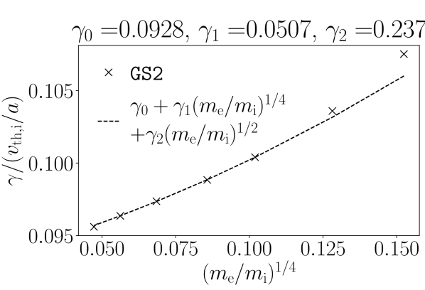
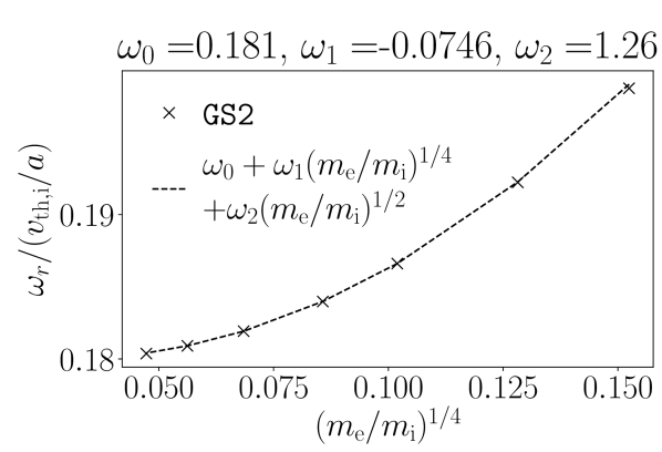
Figure 22: Plots of the growth rate $\gamma$ (left) and real frequency $\omega_{{\rm{r}}}$ (right) as a function of $\left({m_{\rm{e}}}/{m_{\rm{i}}}\right)^{1/4}$, for $\nu_{\ast}=1.22$ (case D of figure 14). We give a quadratic fit to demonstrate that the dependence of $\gamma$ and $\omega_{{\rm{r}}}$ on $\left({m_{\rm{e}}}/{m_{\rm{i}}}\right)^{1/4}$ is consistent with a $\left({m_{\rm{e}}}/{m_{\rm{i}}}\right)^{1/4}$ expansion if a $\left({m_{\rm{e}}}/{m_{\rm{i}}}\right)^{1/2}$ term is included.

Finally, in figure 22 we plot the growth rate $\gamma$ and the real frequency $\omega_{{\rm{r}}}$ as a function of $\left({m_{\rm{e}}}/{m_{\rm{i}}}\right)^{1/4}$. The asymptotic expansion for the collisional small-tail mode is carried out in powers of $\left({m_{\rm{e}}}/{m_{\rm{i}}}\right)^{1/4}$. Hence, we would expect the leading corrections to the frequency to scale as $\omega^{(1/2)}/\omega^{(0)}\sim\left({m_{\rm{e}}}/{m_{\rm{i}}}\right)^{1/4}$, with a subleading correction scaling like $\omega^{(1)}/\omega^{(0)}\sim\left({m_{\rm{e}}}/{m_{\rm{i}}}\right)^{1/2}$. Possibly consistent with this, in figure 22 we see that the coefficients of plausible quadratic fits have parameters $\gamma_{0}$ and $\gamma_{2}$ ($\omega_{0}$ and $\omega_{2}$) of order unity, with $\gamma_{1}$ ($\omega_{1}$) unexpectedly small. This may indicate the need for a more complicated asymptotic theory, or simply that the $\left({m_{\rm{e}}}/{m_{\rm{i}}}\right)^{1/4}$ correction is small in this example.

6.3 The transition between the large-tail and small-tail modes

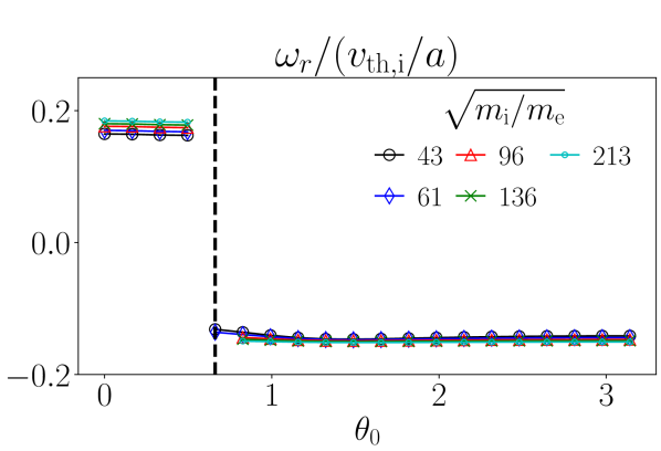
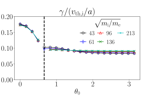
Figure 23: The real frequency $\omega_{{\rm{r}}}$ (left) and growth rate $\gamma$ (right) as a function of $\theta_{0}$ and $\left({m_{\rm{i}}}/{m_{\rm{e}}}\right)^{1/2}$, for $a\nu_{\rm{ee}}/v_{\rm{th,i}}=5.21\times 10^{-3}$, $a/L_{T_{\rm{e}}}=3.45$ and $a/L_{T_{\rm{i}}}=2.3$. The discontinuity in $\omega_{{\rm{r}}}$ indicates a transition between different instability branches. Modes to the left of the dashed line are small-tail modes (driven by trapped electrons and ions), whereas modes to the right of the dashed line are large-tail modes (driven by passing electrons). Note that $\omega_{{\rm{r}}}$ and $\gamma$ are approximately independent of $\theta_{0}$ for the large-tail modes over a wide range of $\theta_{0}$.

In the results that we have presented in the previous sections, we have focused on examples where either a large-tail mode or a small-tail mode is clearly dominant. However, in practice it is possible to find cases where these different asymptotic branches have similar growth rates at the same $k_{y}$ and $\theta_{0}$, meaning that a transition can be observed with the variation of some parameter. To illustrate this, we consider modes with $k_{y}\rho_{\rm{th,i}}=0.5$, $a/L_{T_{\rm{e}}}=3.45$, $a/L_{T_{\rm{i}}}=2.3$, and a electron collisionality of $a\nu_{\rm{ee}}/v_{\rm{th,i}}=5.21\times 10^{-3}$. Figure 23 shows the real frequency $\omega_{{\rm{r}}}$ and growth rate $\gamma$ of these modes as a function of $\theta_{0}$, for different values of $\left({m_{\rm{i}}}/{m_{\rm{e}}}\right)^{1/2}$ at fixed $a\nu_{\rm{ee}}/v_{\rm{th,i}}$. There is clear discontinuity in $\omega_{{\rm{r}}}$, indicating a transition between different mode branches. By examining the eigenmodes using the techniques of sections 6.1 and 6.2, we verify that the modes to the right of the dashed line are collisionless large-tail modes. In contrast, we identify that the modes to the left of the dashed line are collisionless small-tail modes. We note that the small-tail mode drifts in the ion diamagnetic direction, whereas the large-tail mode drifts in the electron diamagnetic direction. As $\left({m_{\rm{i}}}/{m_{\rm{e}}}\right)^{1/2}$ increases, the $\gamma$ and $\omega_{{\rm{r}}}$ of the large tail mode become independent of $\theta_{0}$, in accordance with the predictions of section 4.4.

We note that initial-value simulations of eigenmodes are challenging to converge when distinct instabilities exist at the same $(k_{y},\theta_{0})$ with the same $\gamma$. The data plotted in figures 23 are for modes where the $\omega_{{\rm{r}}}$ and $\gamma$ are converged to 0.5% (compared to values averaged over a $5a/v_{\rm{th,i}}$ window) after $500a/v_{\rm{th,i}}$. A time step size of $\Delta t=0.1a/v_{\rm{th,i}}$ was found to be adequate to resolve the collisionless modes featured in this section. The number of $2\pi$ elements of the ballooning chain was taken to be $n_{2\pi}=65\sqrt{m_{{\rm{i}}}/m_{{\rm D}}}$.

7 Discussion

In the conventional treatment of the nonadiabatic electron response in modes with binormal wavenumbers on the scale of the ion thermal gyroradius, i.e., in modes with $k_{y}\rho_{\rm{th,i}}\sim 1$, rapid electron parallel streaming is assumed to imply that the nonadiabatic response of passing electrons should be small. This assumption leads to the usual ITG-driven modes and TEMs where the nonadiabatic passing electron response is subdominant. However, several numerical investigations have revealed the existence of long-wavelength modes with extended ballooning tails where the nonadiabatic passing electron response appears to play a significant role, see, e.g., [12, 13, 15, 16, 17, 18, 25, 27]. In terms of a wavenumber-space description, these electron-driven modes are fluctuations with large radial wave numbers, i.e., $k_{r}\rho_{\rm{th,i}}\gg 1$. In the real-space description, these modes are fine-scale fluctuations with significant amplitudes near mode-rational flux surfaces. Examples of these modes may be found in the core of tokamaks [12, 13], and in the pedestal [15]. Qualitatively, micro-tearing modes in tokamaks share the same features as the extended electrostatic modes in [12, 13, 15], with both extended ballooning tails and an ETG drive [16, 17, 18].

In this paper, we show that it is possible to obtain an asymptotic theory for novel electron-response-driven $k_{y}\rho_{\rm{th,i}}\sim 1$ modes by assuming that the nonadiabatic response of passing electrons cannot be neglected, and by carefully considering the regions in the mode with large $k_{r}$. The physics of these novel modes turn out to be dominated by the physics at $k_{r}\rho_{\rm{th,i}}\gg 1$, and surprisingly, the nonadiabatic ion response is unimportant (but not small). When the nonadiabatic-electron-response-driven modes are unstable, their growth rate is expected to be insensitive to the exact details of the magnetic geometry, because the leading-order equations for the mode contain only poloidal-angle-averaged geometric quantities. As a corollary, the growth rate of the mode is expected to be independent of $\theta_{0}$. Hence, extended, electrostatic electron-driven modes may be insensitive to equilibrium flow shear, driving turbulence even when the more familiar ITG modes and TEMs are flow-shear stabilised. This observation may be important for projected tokamaks scenarios that rely on equilibrium flow shear to stabilise microinstabilities, cf. [47].

We identify two limits where there are simple orderings. First, we examine the collisionless limit, where $qR_{0}\nu_{\rm{ee}}/v_{\rm{th,e}}\sim\left(m_{\rm{e}}/m_{\rm{i}}\right)^{1/2}\ll 1$, the radial wave number satisfies $k_{r}\rho_{\rm{th,e}}\sim 1$, and the fundamental expansion parameter is $\left(m_{\rm{e}}/m_{\rm{i}}\right)^{1/2}\ll 1$. In the collisionless ordering, the extent of the mode is set by the physics of electron free streaming, and electron finite Larmor radius and electron finite orbit width effects. Second, we examine the collisional limit where $qR_{0}\nu_{\rm{ee}}/v_{\rm{th,e}}\sim 1$, the radial wave number satisfies $k_{r}\rho_{\rm{th,e}}\sim\left({m_{\rm{e}}}/{m_{\rm{i}}}\right)^{1/4}$, and the fundamental expansion parameter is $\left({m_{\rm{e}}}/{m_{\rm{i}}}\right)^{1/4}\ll 1$. In the collisional ordering, the extent of the mode is set by parallel and perpendicular classical and neoclassical diffusion. We note that the collisionless and collisional orderings for the extent of the electrostatic modes considered in this paper are reminiscient of the collisionless and semicollisional orderings for the size of a tearing layer in a sheared magnetic field, see, for example [48, 49, 39, 50, 51].

We derive scaling laws for the relative sizes of the electron and ion responses in the $k_{r}\rho_{\rm{th,i}}\sim 1$ and $k_{r}\rho_{\rm{th,i}}\gg 1$ regions of the ballooning mode. To confirm our analytically derived scalings, we use the gyrokinetic stability code GS2 to perform a series of linear simulations for a range of normalised electron collisionality $\nu_{\ast}=qR_{0}\nu_{\rm{ee}}/\epsilon^{3/2}v_{\rm{th,e}}$, and a range of $m_{{\rm{e}}}/m_{{\rm{i}}}$. We identify parameters where a novel passing-electron-driven mode is the fastest unstable mode. We present two relatively clean examples of the passing-electron-driven mode: a collisionless case and a collisional case. We perform the same analysis for an ITG mode, and verify the scalings for the subdominant nonadiabatic electron response.

Although the theory presented here neglects electromagnetic fluctuations, many features of these novel electrostatic modes are common to micro-tearing modes. We speculate that some classes of micro-tearing modes may be well described by a collisionless $\left(m_{\rm{e}}/m_{\rm{i}}\right)^{1/2}\rightarrow 0$ theory or collisional $\left({m_{\rm{e}}}/{m_{\rm{i}}}\right)^{1/4}\rightarrow 0$ theory similar to the theories presented in this paper. Development of these asymptotic theories provides not just physical insight, but also the possibility of performing reduced linear simulations of nonadiabatic-electron-response-driven modes. Simulations of extended ballooning modes can be expensive in comparison to simulations of familiar ITG-driven modes: a reduction of the size of the problem by removing the geometric $2\pi$ poloidal-angle scale from the gyrokinetic equations may be an advantage. We anticipate that the need for computational efficiency in simulating extended ballooning modes will become more urgent in light of recent work [52] that suggests high-$\beta$ spherical tokamak reactor equilibria may be unstable to extended micro-tearing modes for a wide range of $k_{y}$.

The nonadiabatic response of passing electrons has recently been shown to be a significant factor in determining the isotope effect [23, 24]. In fact, [24] argues that changes in a $\left(m_{\rm{e}}/m_{\rm{i}}\right)^{1/2}$-small passing electron nonadiabatic response can lead to $\Or\left(1\right)$ changes in the heat fluxes as a result of the divergent asymptotic expansion in $\left(m_{\rm{e}}/m_{\rm{i}}\right)^{1/2}$. In this paper we have seen that, in linear modes, the nonadiabatic response of passing electrons does not need to be small in $\left(m_{\rm{e}}/m_{\rm{i}}\right)^{1/2}$. Indeed, it is not even obvious that an expansion should be carried out in $\left(m_{\rm{e}}/m_{\rm{i}}\right)^{1/2}$. Instead, $\left({m_{\rm{e}}}/{m_{\rm{i}}}\right)^{1/4}$ could be the relevant expansion parameter for sufficiently large collisionality. This is an important observation, because, in practice, $\left({m_{\rm{e}}}/{m_{\rm{i}}}\right)^{1/4}\approx 1/8$ is likely to a be worse expansion parameter than $\left(m_{\rm{e}}/m_{\rm{i}}\right)^{1/2}\approx 1/60$. For sufficiently large collisionality, nonasymptotic behaviour may perhaps be observed because the physical value of $\left({m_{\rm{e}}}/{m_{\rm{i}}}\right)^{1/4}$ is not small enough. Whilst we do not develop a nonlinear theory in this paper, we speculate that the isotope effect may well be the result of the nonadiabatic response of passing electrons in $k_{r}\rho_{\rm{th,i}}\gg 1$ narrow layers regulating turbulent transport.

The impact of electron-driven narrow radial layers in nonlinearly saturated turbulence is the subject of active research. Studies of turbulence using DNS have demonstrated that the nonadiabatic response of passing electrons in narrow layers near the mode-rational flux surfaces can have a significant impact on turbulence saturation levels and fluxes, see, e.g., [12, 53, 13, 26, 25, 27]. We note that electron-driven narrow radial layers are not necessarily associated with mode-rational surfaces. In fact, narrow radial structures formed by ion-gyroradius-scale toroidal ETG modes near the top and bottom of the tokamak [15] have recently been observed to regulate the fluxes in nonlinear DNS of ETG-driven pedestal turbulence [54]. The pedestal toroidal ETG modes driving these structures rely on magnetic drift resonances and have large radial wave numbers as a result of the large gradients of density and temperature, but, in contrast to the modes featured in this paper, they rely on favourable local magnetic geometry and are relatively localised in the ballooning angle. As mentioned in the introduction, electron-tail modes with extended ballooning eigenfunctions may nonetheless be observed in the pedestal at very long binormal wavelengths (see Appendix B of [15]): extended eigenfunctions arise naturally when there is a separation between the frequencies associated with free streaming and the drives of instability.

Further evidence for the importance of the nonadiabatic response of passing electrons in narrow layers may be found in DNS that bridge $k_{y}\rho_{\rm{th,i}}\sim 1$ to $k_{y}\rho_{\rm{th,e}}\sim 1$ scales: entropy transfer analysis suggests that the nonadiabatic response of passing electrons mediates the backreaction of $k_{y}\rho_{\rm{th,e}}\sim 1$ eddies on $k_{y}\rho_{\rm{th,i}}\sim 1$ turbulence, via $k_{r}\rho_{\rm{th,i}}\gg 1$ narrow layers [6]. These observations suggest that theories of turbulence that attempt to capture the $\left(m_{\rm{e}}/m_{\rm{i}}\right)^{1/2}\rightarrow 0$ limit may need to be modified to include the effects of electrons in narrow radial layers on saturation: this includes theories of turbulence on $k_{y}\rho_{\rm{th,i}}\sim 1$ scales in isolation (cf. [34]) and theories of cross-scale interactions between $k_{y}\rho_{\rm{th,i}}\sim 1$ and $k_{y}\rho_{\rm{th,e}}\sim 1$ scales (cf. [33, 46]).

Finally, we note that whilst the results presented here are specialised to an axisymmetric tokamak by virtue of using the identity (22), we speculate that a similar theory to the one we present might be obtained for stellarator geometries. Physically, passing-electron-driven resonances at mode rational surfaces can arise in tokamaks due to the vanishing average radial magnetic drift – undisturbed passing particles may return many times to the same location on the flux surface. Stellarator geometries also guarantee that the average radial magnetic drift of passing particles is zero [58], possibly allowing for similar passing-electron-driven modes at rational surfaces. In a stellarator, trapped particles only have zero average radial magnetic drift if the geometry is omnigeneous [55, 56, 57, 58, 59, 60]. As a consequence, in an arbitrary stellarator trapped particles may act to disturb passing-electron-drive modes by dragging passing particles off rational surfaces through collisions – we note that this effect would disappear in the $\nu_{\ast}\gg 1$ limit in which trapped particles cannot complete an orbit.

The authors are grateful for productive discussions with N. Christen, O. Beeke, B. Patel, J. Maurino-Alperovich, S. Trinczek, C. M. Roach, B. F. McMillan, A. A. Scheckochihin, W. Dorland, J. Ball, S. Brunner, I. Calvo, J. M. García Regaña, H. Thienpondt, M. Abazorius, J. Ruiz Ruiz, D. St-Onge, G. Acton and V. Hall-Chen. The simulations were performed using the GS2 branch https://bitbucket.org/gyrokinetics/gs2/branch/ms_pgelres, with the latest revision at the time of writing being commit ade5780. The GS2 input files used to perform the gyrokinetic simulations in this study are publicly available at https://doi.org/10.5287/bodleian:xr5ZApXYm, alongside scripts used to calculate the neoclassical transport coefficients. This work has been carried out within the framework of the EUROfusion Consortium and has received funding from the Euratom research and training programme 2014-2018 and 2019-2020 under grant agreement No 633053, and from EPSRC [Grant Numbers EP/T012250/1 and EP/R034737/1]. The views and opinions expressed herein do not necessarily reflect those of the European Commission. The author acknowledges the use of the EUROfusion High Performance Computer (Marconi-Fusion) under projects MULTEI and OXGK, ARCHER through the Plasma HEC Consortium EPSRC Grant Numbers EP/L000237/1 and EP/R029148/1 under the projects e281-gs2 and e607, the JFRS-1 supercomputer at IFERC-CSC in Rokkasho Fusion Institute of QST (Aomori, Japan), and software support through the Plasma-CCP Network under EPSRC Grant Number EP/M022463/1.

Appendix A A detailed analysis of the ion response for large $\theta$

In this appendix, we give a detailed analysis of the nonadiabatic ion response at large ballooning $\theta$. This discussion will illustrate in more detail how the hyperbolic ion gyrokinetic equation, equation (4) with $s={\rm i}$, reduces to the local algebraic equation (53) in the electron-dominated tail of the ballooning mode.

We note that, for large $\theta$, the leading-order ion gyrokinetic equation has the form

$$\sigma\frac{\partial h_{{\rm{i}}}}{\partial\theta}+P(\theta)h_{{\rm{i}}}=S(\theta),$$ (124)

where the source $S={\rm{i}}\left(\omega_{\ast,{\rm{i}}}-\omega\right)J_{0{\rm{i}}}F_{0i}\;Z_{\rm{i}}e\phi{}/T_{\rm{i}}|v_{\|}|\bm{b}\!\cdot\!\nabla\theta$, and the factor $P\gg 1$. We argue, in section 4.2.1, that in the collisionless limit

$$P=\frac{1}{|v_{\|}|\bm{b}\!\cdot\!\nabla\theta}\left(\frac{k_{\alpha}^{2}{q^{\prime}}^{2}|\nabla\psi|^{2}\theta^{2}v^{2}}{4\Omega_{\rm{i}}^{2}}\left(\nu_{\|,{\rm i}}\lambda B+\frac{\nu_{\perp,{\rm i}}}{2}\left(2-\lambda B\right)\right)-{\rm{i}}k_{\alpha}q^{\prime}\theta\bm{v}_{\rm{M,i}}\cdot\nabla\psi\right),$$ (125)

whereas, in section 5.1.1, we argue that in the collisional limit

$$P={\frac{k_{\alpha}^{2}{q^{\prime}}^{2}|\nabla\psi|^{2}\theta^{2}v^{2}}{4\Omega_{\rm{i}}^{2}|v_{\|}|\bm{b}\!\cdot\!\nabla\theta}\left(\nu_{\|,{\rm i}}\lambda B+\frac{\nu_{\perp,{\rm i}}}{2}\left(2-\lambda B\right)\right)},$$ (126)

i.e., we can neglect the term due to the radial magnetic drift. In solving for the ion response, we have no need to distinguish between $\theta$ and $\chi$ – this distinction is only a requirement for solving for the electron response. For simplicity, in the subsequent algebra we drop the usage of $\chi$. In writing equation (124), we have emphasised the $\theta$ dependence of $S$ and $P$, and we have neglected the differential terms of the ion gyrokinetic collision operator, and the terms due to the time derivative of $h_{{\rm{i}}}$, and the precessional magnetic drift. These terms can be neglected because $\theta\gg 1$, $k_{y}\rho_{\rm{th,i}}\sim 1$ and $\omega\sim v_{\rm{th,i}}/a$, and hence the leading terms are large, i.e., $P\gg 1$. Note that the real part of $P$ is positive, i.e., $\Re\left[P\right]>0$.

We consider the solution of equation (124) for $\theta>0$. Integrating equation (124) directly, we find that, for forward going particles ($\sigma=1$),

$$h_{{\rm{i}}}=\int^{\theta}_{0}S(\theta^{\prime\prime})\exp{\left[-\int^{\theta}_{\theta^{\prime\prime}}P(\theta^{\prime})d\theta^{\prime}\right]}d\theta^{\prime\prime}+h_{{\rm{i}}}(\theta=0,\sigma=1)\exp{\left[-\int^{\theta}_{0}P(\theta^{\prime})d\theta^{\prime}\right]}.$$ (127)

For backward-going particles ($\sigma=-1$), we find that

$$h_{{\rm{i}}}=\int^{\infty}_{\theta}S(\theta^{\prime\prime})\exp{\left[-\int_{\theta}^{\theta^{\prime\prime}}P(\theta^{\prime})d\theta^{\prime}\right]}d\theta^{\prime\prime},$$ (128)

where we have used $h_{{\rm{i}}}(\theta=\infty,\sigma=-1)=0$ as a boundary condition. Inspecting the solutions (127) and (128), we note that there are two components: a “local” solution involving $S$, and an exponentially decaying solution (proportional to $h_{{\rm{i}}}(\theta=0,\sigma=1)$) due to the outgoing particles from $\theta=0$. The exponentially decaying part of the solution gives rise to the logarithmic boundary layer referred to in G. In this discussion, we can neglect the exponentially decaying part of the ion response, because the electron tail at large $\theta$ generates its own potential that drives the ions via the “local” response.

We now consider the form of the local solution when $P\gg 1$ and $\Re[P]>0$, and the integrals can be treated using the standard Laplace method [61]. We treat the case of $\sigma=1$ explicitly. First, we note that the dominant contributions to the integrals in equation (127) come from where $\theta\simeq\theta^{\prime\prime}$. In this region, we write

$$\exp{\left[-\int^{\theta}_{\theta^{\prime\prime}}P(\theta^{\prime})d\theta^{\prime}\right]}=\exp{\left[-P(\theta)(\theta-\theta^{\prime\prime})\right]}\left(1+\Or\left(\frac{1}{P}\frac{\partial P}{\partial\theta}(\theta-\theta^{\prime\prime})\right)\right),$$ (129)

which is accurate provided that $(\theta-\theta^{\prime\prime})/\theta\ll 1$. We introduce a parameter $\delta$, so that we can write

$$h_{{\rm{i}}}=I_{0}+I_{\delta}$$ (130)

with

$$I_{0}=\int^{\theta}_{\theta-\delta}S(\theta^{\prime\prime})\exp{\left[-\int^{\theta}_{\theta^{\prime\prime}}P(\theta^{\prime})d\theta^{\prime}\right]}d\theta^{\prime\prime},$$ (131)

and

$$I_{\delta}=\int^{\theta-\delta}_{0}S(\theta^{\prime\prime})\exp{\left[-\int^{\theta}_{\theta^{\prime\prime}}P(\theta^{\prime})d\theta^{\prime}\right]}d\theta^{\prime\prime}.$$ (132)

We can use the appoximation (129) in $I_{0}$ provided $\delta/\theta\ll 1$. Using (129), the leading contribution to $I_{0}$ is given by

$$I_{0}=\int^{\theta}_{\theta-\delta}S(\theta)\exp{\left[-P(\theta)(\theta-\theta^{\prime\prime})\right]}d\theta^{\prime\prime}.$$ (133)

Evaluating the integral, we find that

$$I_{0}=\frac{S(\theta)}{P(\theta)}\left(1-\exp{\left[-P(\theta)\delta\right]}\right).$$ (134)

Taking $\delta$ such that $\Re[P]\delta\gg 1$ (consistent with $\delta/\theta\ll 1$), we find that, to leading order,

$$h_{{\rm{i}}}=\frac{S(\theta)}{P(\theta)},$$ (135)

where we have used the smallness of $\exp{\left[-P(\theta)\delta\right]}$ to neglect $I_{\delta}$. An analogous calculation can be performed for $\sigma=-1$, with the result that $h_{{\rm{i}}}$ satisfies (135) for both signs of the velocity. The result (135) is identical in form to equations (53). We have demonstrated that, although the ion gyrokinetic equation is hyperbolic, the fact that $P\gg 1$ means that parallel streaming is unable to effectively propagate information at large $\theta$, and hence, the nonadiabatic response of ions is local in ballooning angle.

Appendix B Obtaining the electron transport equations in the collisional inner region

In this section we calculate the forms of the transport equations that describe the electron response in the in the $\left({m_{\rm{e}}}/{m_{\rm{i}}}\right)^{1/4}\rightarrow 0$ limit, for $k_{y}\rho_{\rm{th,i}}\sim 1$ modes with $qR_{0}\nu_{\rm{ee}}/v_{\rm{th,e}}\sim 1$. We note that, in the ordering for the collisional inner region, ${\chi}\sim\left({m_{\rm{i}}}/{m_{\rm{e}}}\right)^{1/4}\gg 1\sim\theta_{0}\gg\lambda_{{\rm{e}}}\sim\left(m_{\rm{e}}/m_{\rm{i}}\right)^{1/2}$, and hence the phase in equation (25) for $H_{\rm{e}}$ becomes

$$\exp{\left[{\rm{i}}\lambda_{{\rm{e}}}(\theta_{0}-\theta)\right]}=\left(1-{\rm{i}}\lambda_{{\rm{e}}}\chi-\frac{\lambda_{{\rm{e}}}^{2}\chi^{2}}{2}+{\rm{i}}\lambda_{{\rm{e}}}\theta_{0}+\Or\left(\left(\frac{m_{\rm{e}}}{m_{\rm{i}}}\right)^{3/4}\right)\right).$$ (136)

In addition, we will need to expand the phase due to the finite Larmor radius $\exp{\left[{\rm{i}}\bm{k}_{\perp}\cdot\bm{\rho}_{e}\right]}$ in the collision operator $C^{\rm{GK}}_{\rm{e}}\left[\cdot\right]$. In the inner region, we find

$$\exp{\left[{\rm{i}}\bm{k}_{\perp}\cdot\bm{\rho}_{e}\right]}=1+{\rm{i}}\bm{k}^{(0)}_{\perp}\cdot\bm{\rho}_{e}-\frac{1}{2}(\bm{k}^{(0)}_{\perp}\cdot\bm{\rho}_{e})^{2}+{\rm{i}}\bm{k}^{(1)}_{\perp}\cdot\bm{\rho}_{e}+\Or\left(\left(\frac{m_{\rm{e}}}{m_{\rm{i}}}\right)^{3/4}\right),$$ (137)

where we note that $\bm{k}^{(0)}_{\perp}\cdot\bm{\rho}_{e}\sim\left({m_{\rm{e}}}/{m_{\rm{i}}}\right)^{1/4}$ and $\bm{k}^{(1)}_{\perp}\cdot\bm{\rho}_{e}\sim\left({m_{\rm{e}}}/{m_{\rm{i}}}\right)^{1/2}$.

The leading order equation for the electron response in the inner region is equation (81). To obtain equation (81) we have used the equations (136) and (137) for the finite-orbit-width and finite-Larmor-radius phases, respectively, and the estimate (79) for $\delta\!\bm{u}_{\rm{i}}$ to simplify the collision operators to the drift-kinetic form. We have also noted that $H^{(0)}_{{\rm{e}}}$ is gyrophase independent, and $C_{\rm{ee}}[\cdot]$ and $\mathcal{L}[\cdot]$ commute with $\left\langle{\cdot}\right\rangle^{\gamma}$.

We follow a H-theorem procedure [40, 32] to solve equation (81): first, we multiply equation (81) by $H^{(0)}_{{\rm{e}}}/F_{0e}$, with the result

$$v_{\|}\bm{b}\!\cdot\!\nabla\theta\frac{\partial}{\partial\theta}\left(\frac{\left(H^{(0)}_{{\rm{e}}}\right)^{2}}{2F_{0e}}\right)=\frac{H^{(0)}_{{\rm{e}}}}{F_{0e}}C_{\rm{ee}}\left[H^{(0)}_{{\rm{e}}}\right]+\frac{H^{(0)}_{{\rm{e}}}}{F_{0e}}\mathcal{L}\left[H^{(0)}_{{\rm{e}}}\right].$$ (138)

Second, we integrate over velocity space

$$\bm{B}\cdot\nabla\theta\frac{\partial}{\partial\theta}\left(\int\frac{v_{\|}}{B}\frac{\left(H^{(0)}_{{\rm{e}}}\right)^{2}}{2F_{0e}}\;d^{3}\bm{v}\right)$$

$$=\int\frac{H^{(0)}_{{\rm{e}}}}{F_{0e}}C_{\rm{ee}}\left[H^{(0)}_{{\rm{e}}}\right]\;d^{3}\bm{v}+\int\frac{H^{(0)}_{{\rm{e}}}}{F_{0e}}\mathcal{L}\left[H^{(0)}_{{\rm{e}}}\right]\;d^{3}\bm{v},$$ (139)

where we have used the form of the velocity integral in $(\varepsilon,\lambda)$ coordinates,

$$\int\left(\cdot\right)\;d^{3}\bm{v}=\sum_{\sigma}\int^{\infty}_{0}\int^{1/B}_{0}\frac{2\pi B\varepsilon}{m_{s}^{2}|v_{\|}|}\left(\cdot\right)\;d\lambda\;d\varepsilon,$$ (140)

and taken the ${\partial}/{\partial\theta}$ derivative through the integral. Finally, we apply the poloidal angle average $\left\langle{\cdot}\right\rangle^{\theta}$, defined by equation (80), to equation (139), and impose periodicity of $H^{(0)}_{{\rm{e}}}$ in $\theta$, to obtain

$$\left\langle{\int\frac{H^{(0)}_{{\rm{e}}}}{F_{0e}}\;C_{\rm{ee}}\left[H^{(0)}_{{\rm{e}}}\right]\;d^{3}\bm{v}}\right\rangle^{\theta}+\left\langle{\int\frac{H^{(0)}_{{\rm{e}}}}{F_{0e}}\;\mathcal{L}\left[H^{(0)}_{{\rm{e}}}\right]\;d^{3}\bm{v}}\right\rangle^{\theta}=0.$$ (141)

The collision operators $C_{\rm{ee}}\left[\cdot\right]$ and $\mathcal{L}\left[\cdot\right]$ have the properties [32]

$$\int\frac{g}{F_{0e}}\;C_{\rm{ee}}\left[g\right]\;d^{3}\bm{v}\leq 0\quad{\rm{and}}\quad\int\frac{g}{F_{0e}}\;\mathcal{L}\left[g\right]\;d^{3}\bm{v}\leq 0,$$ (142)

respectively. Collisions always increase the entropy of the system. The equality $\int(g/F_{0e})\;C_{\rm{ee}}\left[g\right]\;d^{3}\bm{v}=0$ is only achieved when $g$ is a perturbed Maxwellian so that $C_{\rm{ee}}\left[g\right]=0$. The equality $\int(g/F_{0e})\;\mathcal{L}\left[g\right]\;d^{3}\bm{v}=0$ is only achieved when $g$ is isotropic in $\bm{v}$ so that $\mathcal{L}\left[g\right]=0$. As a consequence of equation (141), we find that $H^{(0)}_{{\rm{e}}}$ satisfies equation (82) with $\delta\!n^{(0)}_{\rm{e}}$ and $\delta\!T^{(0)}_{\rm{e}}$ functions of $\theta$ and $\chi$ to be determined. Returning to equation (81), we now find that $H^{(0)}_{{\rm{e}}}$ must also satisfy $v_{\|}\bm{b}\!\cdot\!\nabla\theta{\partial H^{(0)}_{{\rm{e}}}}/{\partial\theta}=0$. For ${\partial H^{(0)}_{{\rm{e}}}}/{\partial\theta}=0$ to hold for all $\varepsilon$, we must have that $\delta\!n^{(0)}_{\rm{e}}$ and $\delta\!T^{(0)}_{\rm{e}}$ are constant in $\theta$, i.e., $\delta\!n^{(0)}_{\rm{e}}$ and $\delta\!T^{(0)}_{\rm{e}}$ have the form given by equation (83).

The first-order equation for the electron response in the inner region takes the form

$$v_{\|}\bm{b}\!\cdot\!\nabla\theta\frac{\partial H^{(1/2)}_{{\rm{e}}}}{\partial\theta}+v_{\|}\bm{b}\!\cdot\!\nabla\theta\frac{\partial H^{(0)}_{{\rm{e}}}}{\partial\chi}=\mathcal{C}\left[H^{(1/2)}_{{\rm{e}}}+{\rm{i}}\lambda_{{\rm{e}}}\chi H^{(0)}_{{\rm{e}}}\right],$$ (143)

where we have used the definition of the drift-kinetic electron collision operator $\mathcal{C}\left[\cdot\right]$, equation (37). To expand the collision operator (28) for electrons, we have used the definition (8), equations (136) and (137), the estimate (79), and the identities

$$\left\langle{{\rm{i}}\bm{k}^{(0)}_{\perp}\cdot\bm{\rho}_{e}\;\mathcal{C}\left[H^{(0)}_{{\rm{e}}}\right]}\right\rangle^{\gamma}=\left\langle{\mathcal{C}\left[{\rm{i}}\bm{k}^{(0)}_{\perp}\cdot\bm{\rho}_{e}\;H^{(0)}_{{\rm{e}}}\right]}\right\rangle^{\gamma}=\mathcal{C}[H^{(0)}_{{\rm{e}}}]=0.$$ (144)

Equation (143) bears a resemblance to the neoclassical drift-kinetic equation in the banana collisionality regime [40, 32]. We note that the term $v_{\|}\bm{b}\!\cdot\!\nabla\theta{\partial H^{(0)}_{{\rm{e}}}}/{\partial\chi}$ plays the role of the equilibrium inductive electric field in the corresponding neoclassical equation. The resemblance can be made explicit by absorbing the $v_{\|}\bm{b}\!\cdot\!\nabla\theta{\partial H^{(0)}_{{\rm{e}}}}/{\partial\chi}$ term into the collision operators by solving the Spitzer-Härm problem, equation (94). It is useful to note that because the collision operator $\mathcal{C}[\cdot]$ is isotropic [32], $H_{\rm{SH}}$ must have the form

$$H_{\rm{SH}}=v_{\|}K_{\rm{SH}}(\varepsilon,\chi)F_{0e},$$ (145)

where $K_{\rm{SH}}$ is a function of $\varepsilon$ and $\chi$. We determine $K_{\rm{SH}}$ in C. Using $H_{\rm{SH}}$, we can rewrite equation (143) in the form of equation (95).

To determine the time evolution of $\delta\!n^{(0)}_{\rm{e}}$ and $\delta\!T^{(0)}_{\rm{e}}$, we continue to the $\Or\left(\left(m_{\rm{e}}/m_{\rm{i}}\right)^{1/2}\right)$ equation. After collecting terms of $\Or\left(\left(m_{\rm{e}}/m_{\rm{i}}\right)^{1/2}\right)$, we find that the equation that determines $H^{(0)}_{{\rm{e}}}$ is

$$v_{\|}\bm{b}\!\cdot\!\nabla\theta\frac{\partial H^{(1)}_{{\rm{e}}}}{\partial\theta}+v_{\|}\bm{b}\!\cdot\!\nabla\theta\frac{\partial H^{(1/2)}_{{\rm{e}}}}{\partial\chi}+{\rm{i}}(\omega_{\rm{M,e}}-\omega^{(0)})H^{(0)}_{{\rm{e}}}$$

$$-\mathcal{C}\left[H^{(1)}_{{\rm{e}}}+{\rm{i}}\lambda_{{\rm{e}}}\chi H^{(1/2)}_{{\rm{e}}}{-}\left(\frac{1}{2}\left(\lambda_{{\rm{e}}}^{2}\chi^{2}+\left\langle{(\bm{k}^{(0)}_{\perp}\cdot\bm{\rho}_{e})^{2}}\right\rangle^{\gamma}\right){+}{\rm{i}}\lambda_{{\rm{e}}}\theta_{0}\right)H^{(0)}_{{\rm{e}}}\right]$$ (146)

$$+{{\rm{i}}\lambda_{{\rm{e}}}\chi\mathcal{C}\left[H^{(1/2)}_{{\rm{e}}}+{\rm{i}}\lambda_{{\rm{e}}}\chi H^{(0)}_{{\rm{e}}}\right]}-\left\langle{\bm{k}^{(0)}_{\perp}\cdot\bm{\rho}_{e}\;\mathcal{C}\left[\bm{k}^{(0)}_{\perp}\cdot\bm{\rho}_{e}\;H^{(0)}_{{\rm{e}}}\right]}\right\rangle^{\gamma}=-{\rm{i}}(\omega_{\ast,{\rm{e}}}-\omega^{(0)})F_{0e}\frac{e\phi^{(0)}}{T_{\rm{e}}},$$

where, to obtain equation (146), we have used equations (136) and (137), estimate (79), identities (144), that $J_{0{\rm{e}}}=1+\Or\left(\left({m_{\rm{e}}}/{m_{\rm{i}}}\right)^{1/2}\right)$ for $\chi\sim\left({m_{\rm{i}}}/{m_{\rm{e}}}\right)^{1/4}$, and that $\mathcal{C}[\cdot]$ and $\left\langle{\cdot}\right\rangle^{\gamma}$ commute.

We can convert equation (146) into equations for $\delta\!n^{(0)}_{\rm{e}}(\chi)$ and $\delta\!T^{(0)}_{\rm{e}}(\chi)$ by multiplying equation (146) by the appropriate velocity space function ($1$ or $\varepsilon/T_{\rm{e}}-3/2$), integrating over velocity space, integrating over $\theta$, and finally imposing on $H^{(1)}_{{\rm{e}}}$ the condition of $2\pi$-periodicity in $\theta$. After performing these operations, and dividing by $n_{\rm{e}}$, the equation for the density moment is

$$\frac{\partial}{\partial\chi}\left(\left\langle{\bm{b}\!\cdot\!\nabla\theta\;\delta\!U^{(1/2)}_{\|,{\rm{e}}}}\right\rangle^{\theta}\right)+{\rm{i}}\left\langle{\omega^{\rm{th}}_{\rm{M,e}}}\right\rangle^{\theta}\left(\frac{\delta\!n^{(0)}_{\rm{e}}}{n_{\rm{e}}}+\frac{\delta\!T^{(0)}_{\rm{e}}}{T_{\rm{e}}}\right)-{\rm{i}}\omega^{(0)}\frac{\delta\!n^{(0)}_{\rm{e}}}{n_{\rm{e}}}$$

$$+\left\langle{{\frac{1}{n_{\rm{e}}}\int{\rm{i}}\lambda_{{\rm{e}}}\chi\;\mathcal{C}\left[H^{(1/2)}_{{\rm{e}}}+{\rm{i}}\lambda_{{\rm{e}}}\chi H^{(0)}_{{\rm{e}}}\right]\;d^{3}\bm{v}}}\right\rangle^{\theta}-\left\langle{\frac{1}{n_{\rm{e}}}\int\left\langle{\bm{k}^{(0)}_{\perp}\cdot\bm{\rho}_{e}\;\mathcal{C}\left[\bm{k}^{(0)}_{\perp}\cdot\bm{\rho}_{e}\;H^{(0)}_{{\rm{e}}}\right]}\right\rangle^{\gamma}\;d^{3}\bm{v}}\right\rangle^{\theta}$$

$$=-{\rm{i}}(\omega^{n}_{\ast,{\rm{e}}}-\omega^{(0)})\frac{e\phi^{(0)}}{T_{\rm{e}}},$$ (147)

where we have defined the effective thermal magnetic drift frequency $\omega^{\rm{th}}_{\rm{M,e}}=\omega_{D}+k_{\alpha}v_{\rm{th,e}}^{2}\bm{b}\!\cdot\!\nabla\theta q^{\prime}I/2\Omega_{\rm{e}}$, the $n^{\rm th}$-order component of the $v_{\|}$ moment of $H^{(0)}_{{\rm{e}}}$

$$\delta\!U^{(n)}_{\|,{\rm{e}}}=\frac{1}{n_{\rm{e}}}\int v_{\|}H^{(n)}_{{\rm{e}}}\;d^{3}\bm{v},$$ (148)

and used that the collision operator $\mathcal{C}\left[\cdot\right]$ satisfies

$$\int\mathcal{C}\left[f\right]\;d^{3}\bm{v}=0$$ (149)

for $f$ an arbitrary function of $\bm{v}$. Similarly, the equation for the electron temperature is

$$\frac{\partial}{\partial\chi}\left(\left\langle{\bm{b}\!\cdot\!\nabla\theta\left(\frac{\delta\!Q^{(1/2)}_{\|,{\rm{e}}}}{n_{\rm{e}}T_{\rm{e}}}+\delta\!U^{(1/2)}_{\|,{\rm{e}}}\right)}\right\rangle^{\theta}\right)+{\rm{i}}\left\langle{\omega^{\rm{th}}_{\rm{M,e}}}\right\rangle^{\theta}\left(\frac{\delta\!n^{(0)}_{\rm{e}}}{n_{\rm{e}}}+\frac{7}{2}\frac{\delta\!T^{(0)}_{\rm{e}}}{T_{\rm{e}}}\right)-{\rm{i}}\frac{3}{2}\omega^{(0)}\frac{\delta\!T^{(0)}_{\rm{e}}}{T_{\rm{e}}}$$

$$+\left\langle{\frac{1}{n_{\rm{e}}}{\int\left(\frac{\varepsilon}{T_{\rm{e}}}-\frac{3}{2}\right){\rm{i}}\lambda_{{\rm{e}}}\chi\;\mathcal{C}\left[H^{(1/2)}_{{\rm{e}}}+{\rm{i}}\lambda_{{\rm{e}}}\chi H^{(0)}_{{\rm{e}}}\right]\;d^{3}\bm{v}}}\right\rangle^{\theta}$$ (150)

$$-\left\langle{\frac{1}{n_{\rm{e}}}\int\left(\frac{\varepsilon}{T_{\rm{e}}}-\frac{3}{2}\right)\left\langle{\bm{k}^{(0)}_{\perp}\cdot\bm{\rho}_{e}\;\mathcal{C}\left[\bm{k}^{(0)}_{\perp}\cdot\bm{\rho}_{e}\;H^{(0)}_{{\rm{e}}}\right]}\right\rangle^{\gamma}\;d^{3}\bm{v}}\right\rangle^{\theta}=-{\rm{i}}\frac{3}{2}\omega^{n}_{\ast,{\rm{e}}}\eta_{\rm{e}}\frac{e\phi^{(0)}}{T_{\rm{e}}},$$

where we have defined the $n^{\rm th}$-order component of the $v_{\|}(\varepsilon/T_{\rm{e}}-5/2)$ moment of $H^{(0)}_{{\rm{e}}}$

$$\delta\!Q^{(n)}_{\|,{\rm{e}}}=\int v_{\|}\left(\varepsilon-\frac{5T_{\rm{e}}}{2}\right)H^{(n)}_{{\rm{e}}}\;d^{3}\bm{v},$$ (151)

and used that the collision operator $\mathcal{C}\left[\cdot\right]$ satisfies

$$\int\left(\frac{\varepsilon}{T_{\rm{e}}}-\frac{3}{2}\right)\mathcal{C}\left[f\right]\;d^{3}\bm{v}=0.$$ (152)

Equations (147) and (150) have simple physical interpretations when written in terms of the leading-order nonzero components of the electron parallel velocity,

$$\delta\!u^{(1/2)}_{\|,{\rm{e}}}=\frac{1}{n_{\rm{e}}}\int v_{\|}(H^{(1/2)}_{{\rm{e}}}+{\rm{i}}\lambda_{{\rm{e}}}\chi H^{(0)}_{{\rm{e}}})\;d^{3}\bm{v},$$ (153)

and electron parallel heat flux

$$\delta\!q^{(1/2)}_{\|,{\rm{e}}}=\int v_{\|}\left(\varepsilon-\frac{5T_{\rm{e}}}{2}\right)(H^{(1/2)}_{{\rm{e}}}+{\rm{i}}\lambda_{{\rm{e}}}\chi H^{(0)}_{{\rm{e}}})\;d^{3}\bm{v},.$$ (154)

After defining the effective parallel velocity and effective parallel heat flux, $\overline{\delta\!u}_{\|}=\left\langle{\bm{b}\!\cdot\!\nabla\theta\;\delta\!u^{(1/2)}_{\|,{\rm{e}}}}\right\rangle^{\theta}/\left\langle{\bm{b}\!\cdot\!\nabla\theta}\right\rangle^{\theta}$ and $\overline{\delta\!q}_{\|}=\left\langle{\bm{b}\!\cdot\!\nabla\theta\;\delta\!q^{(1/2)}_{\|,{\rm{e}}}}\right\rangle^{\theta}/\left\langle{\bm{b}\!\cdot\!\nabla\theta}\right\rangle^{\theta}$, respectively, we obtain equations (85) and (86).

Appendix C Spitzer-Härm component of the parallel diffusion collisional terms

In order to evaluate the parallel flow and neoclassical perpendicular diffusion terms in equations (85) and (86), we need to solve equation (94) for $H_{\rm{SH}}$. To solve for $H_{\rm{SH}}$, we first note that the collision operators $C_{\rm{ee}}[\cdot]$ and $\mathcal{L}[\cdot]$, defined in equations (6) and (9), respectively, are isotropic operators [32], and hence $H_{\rm{SH}}$ may be assumed to have the form given in equation (145). Second, we note that equation (94) is linear in $\delta\!n^{(0)}_{\rm{e}}$ and $\delta\!T^{(0)}_{\rm{e}}$. Third, we may express the $\varepsilon$ dependence of $K_{\rm{SH}}$ in a convenient basis of polynomials. Hence, $K_{\rm{SH}}$ is given by

$$K_{\rm{SH}}=\bm{b}\!\cdot\!\nabla\theta\frac{\partial}{\partial\chi}\left(\frac{\delta\!n^{(0)}_{\rm{e}}}{n_{\rm{e}}}\right)f_{\rm SH}(\hat{x})+\bm{b}\!\cdot\!\nabla\theta\frac{\partial}{\partial\chi}\left(\frac{\delta\!T^{(0)}_{\rm{e}}}{T_{\rm{e}}}\right)g_{\rm SH}(\hat{x}),$$ (155)

where

$$f_{\rm SH}(\hat{x})=\sum_{p=0}a_{p}L^{3/2}_{p}(\hat{x}),$$ (156)

and

$$g_{\rm SH}(\hat{x})=\sum_{p=0}c_{p}L^{3/2}_{p}(\hat{x}),$$ (157)

with $\hat{x}=\varepsilon/T_{\rm{e}}=v^{2}/v_{\rm{th,e}}^{2}$, $L^{3/2}_{p}(\hat{x})$ the $p^{\rm{th}}$ generalised Laguerre polynomial $L^{j}_{p}(\hat{x})$ of index $j=3/2$, and $a_{p}$ and $c_{p}$ coefficients to be determined. The generalised Laguerre polynomials of index $j=3/2$ are particularly convenient for this problem because we will be able to exploit the orthogonality relation [32]

$$\int^{\infty}_{0}L^{j}_{p}(\hat{x})L^{j}_{q}(\hat{x})\exp{\left[-\hat{x}\right]}\hat{x}^{j}d\hat{x}=\frac{\Gamma(p+j+1)}{p!}\delta_{p,q},$$ (158)

where $\Gamma(j)=\int^{\infty}_{0}\hat{x}^{j-1}\exp{\left[-\hat{x}\right]}d\hat{x}$ is the Gamma function, and $\delta_{p,q}$ is the Kronecker delta. The polynomial $L^{j}_{p}(\hat{x})$ may be obtained from the generating function [32]

$$G(\hat{x},z)=\frac{\exp{\left[-\hat{x}z/(1-z)\right]}}{(1-z)^{j+1}}=\sum_{p=0}z^{p}L^{j}_{p}(\hat{x}).$$ (159)

With the form of $K_{\rm{SH}}$ given by equation (155), the problem (94) may be cast into two separate Spitzer problems for $f_{\rm SH}$ and $g_{\rm SH}$,

$$v_{\|}L^{3/2}_{0}F_{0e}=\mathcal{C}\left[v_{\|}f_{\rm SH}F_{0e}\right],$$ (160)

and

$$v_{\|}(L^{3/2}_{0}-L^{3/2}_{1})F_{0e}=\mathcal{C}\left[v_{\|}g_{\rm SH}F_{0e}\right],$$ (161)

where we have used the first two generalised Laguerre polynomials, $L^{3/2}_{0}(\hat{x})=1$ and $L^{3/2}_{1}(\hat{x})=5/2-\hat{x}$. We solve equations (160) and (161) by converting them into matrix equations for the coefficients $a_{p}$ and $c_{p}$, respectively. To do this, we define an inner product $\left\langle\cdot\middle|\cdot\right\rangle$ acting on velocity space functions $f=f(\bm{v})$ and $g=g(\bm{v})$ by

$$\left\langle f\middle|g\right\rangle=\int\frac{f(\bm{v})g(\bm{v})}{F_{0e}}\;d^{3}\bm{v},$$ (162)

and we take the inner product of equations (160) and (161) with the function $v_{\|}L^{3/2}_{q}F_{0e}$. To perform the velocity integrals, we use the velocity coordinates $(\hat{x},\xi,\gamma)$, where $\xi=v_{\|}/v$, and we recall that $\gamma$ is the gyrophase. The velocity integral in these coordinates becomes

$$\int\left(\cdot\right)\;d^{3}\bm{v}=\int^{2\pi}_{0}\int^{1}_{-1}\int^{\infty}_{0}\left(\cdot\right)\;\frac{v_{\rm{th,e}}^{3}}{2}\sqrt{\hat{x}}\;d\hat{x}\;d\xi\;d\gamma.$$ (163)

Using the orthogonality relation (158), we find that the matrix form of equation (160) is

$$\sum_{q}\left(\nu_{\rm{ee}}C_{p,q}+\nu_{\rm{ei}}\mathcal{L}_{p,q}\right)a_{q}=-\delta_{0,p},$$ (164)

where the matrix elements $C_{p,q}$ and $\mathcal{L}_{p,q}$ are defined by

$$C_{p,q}=-\frac{2}{n_{\rm{e}}\nu_{\rm{ee}}}\left\langle\hat{x}^{1/2}\xi F_{0e}L^{3/2}_{p}\middle|C_{\rm{ee}}\left[\hat{x}^{1/2}\xi F_{0e}L^{3/2}_{q}\right]\right\rangle$$ (165)

and

$$\mathcal{L}_{p,q}=-\frac{2}{n_{\rm{e}}\nu_{\rm{ei}}}\left\langle\hat{x}^{1/2}\xi F_{0e}L^{3/2}_{p}\middle|\mathcal{L}\left[\hat{x}^{1/2}\xi F_{0e}L^{3/2}_{q}\right]\right\rangle,$$ (166)

respectively. Similarly, we find that the matrix form of equation (161) is

$$\sum_{q}\left(\nu_{\rm{ee}}C_{p,q}+\nu_{\rm{ei}}\mathcal{L}_{p,q}\right)c_{q}=\frac{5}{2}\delta_{1,p}-\delta_{0,p}.$$ (167)

To solve the problem, we invert the matrix equations (164) and (167). In practice, we must include a finite number of polynomials, with the series truncated at a finite $p=N$. Velocity moments of $H_{\rm{SH}}$ will depend only on low-order coefficients $a_{p}$ and $c_{p}$, and so only a few polynomials are required before convergence is reached. This same solution may be obtained using a variational method [32].

Although the calculation is tedious, it is relatively straightforward to calculate the matrix elements $C_{p,q}$ and $\mathcal{L}_{p,q}$ using the generating function $G(\hat{x},z)$. Truncating the series at polynomial order $N=4$, we find the coefficient matrices (cf. [31, 32])

03/445/16309/128885/512015/32309/1285657/102420349/4096035/128885/51220349/4096149749/16384),𝑪2fragments fragments 03/445/16309/128885/512015/32309/1285657/102420349/4096035/128885/51220349/4096149749/16384\displaystyle\bm{C}=\sqrt{2}\left(\begin{tabular}[]{ccccc}0&0&0&0&0\\ 0&1&3/4&15/32&35/128\\ 0&3/4&45/16&309/128&885/512\\ 0&15/32&309/128&5657/1024&20349/4096\\ 0&35/128&885/512&20349/4096&149749/16384\\ \end{tabular}\right),

00000013/415/3235/12800000013/415/3235/128 (173)

and

3/213/469/16165/321505/25615/869/16433/641077/12810005/102435/16165/321077/1282957/25628257/2048315/1281505/25610005/102428257/2048288473/16384).𝓛fragments 3/213/469/16165/321505/25615/869/16433/641077/12810005/102435/16165/321077/1282957/25628257/2048315/1281505/25610005/102428257/2048288473/16384\displaystyle\bm{\mathcal{L}}=\left(\begin{tabular}[]{ccccc}1&3/2&15/8&35/16&315/128\\ 3/2&13/4&69/16&165/32&1505/256\\ 15/8&69/16&433/64&1077/128&10005/1024\\ 35/16&165/32&1077/128&2957/256&28257/2048\\ 315/128&1505/256&10005/1024&28257/2048&288473/16384\\ \end{tabular}\right).

13/215/835/16315/12813/215/835/16315/128 (179)

To illustrate the final result of the calculation for a simple case, we solve equations (164) and (167) for a hydrogenic plasma with $Z_{\rm{i}}=1$, i.e., $\nu_{\rm{ei}}=\nu_{\rm{ee}}$. To three decimal places, we find that the coefficients $\{a_{n}\}$ and $\{c_{n}\}$ are

$$\left(\begin{tabular}[]{c}$a_{0}$\\ $a_{1}$\\ $a_{2}$\\ $a_{3}$\\ $a_{4}$\\ \end{tabular}\right)=\frac{1}{\nu_{\rm{ei}}}\left(\begin{tabular}[]{c}-1.969\\ 0.559\\ 0.017\\ 0.016\\ 0.027\\ \end{tabular}\right),$$ (190)

and

$$\left(\begin{tabular}[]{c}$c_{0}$\\ $c_{1}$\\ $c_{2}$\\ $c_{3}$\\ $c_{4}$\\ \end{tabular}\right)=\frac{1}{\nu_{\rm{ei}}}\left(\begin{tabular}[]{c}-3.366\\ 2.226\\ -0.635\\ 0.095\\ 0.003\\ \end{tabular}\right),$$ (201)

respectively.

To calculate the parallel flow and the neoclassical perpendicular diffusion terms, we need to evaluate velocity integrals of the form

$$\int v_{\|}H_{\rm{SH}}\;d^{3}\bm{v}=\frac{n_{\rm{e}}v_{\rm{th,e}}^{2}}{2}\bm{b}\!\cdot\!\nabla\theta\left(a_{0}\frac{\partial}{\partial\chi}\left(\frac{\delta\!n^{(0)}_{\rm{e}}}{n_{\rm{e}}}\right)+c_{0}\frac{\partial}{\partial\chi}\left(\frac{\delta\!T^{(0)}_{\rm{e}}}{T_{\rm{e}}}\right)\right),$$ (202)

and

$$\int v_{\|}\left(\frac{v^{2}}{v_{\rm{th,e}}^{2}}-\frac{5}{2}\right)H_{\rm{SH}}\;d^{3}\bm{v}$$ (203)

$$=\frac{5n_{\rm{e}}v_{\rm{th,e}}^{2}}{4}\bm{b}\!\cdot\!\nabla\theta\left(a_{1}\frac{\partial}{\partial\chi}\left(\frac{\delta\!n^{(0)}_{\rm{e}}}{n_{\rm{e}}}\right)+c_{1}\frac{\partial}{\partial\chi}\left(\frac{\delta\!T^{(0)}_{\rm{e}}}{T_{\rm{e}}}\right)\right).$$

Appendix D Classical perpendicular diffusion collisional terms

The collision integrals appearing in the definitions of the classical fluxes $\overline{\delta\!\Gamma}_{\rm C}$ and $\overline{\delta\!q}_{\rm C}$, equations (90) and (91), respectively, have the structural form

$$\int g(v)\bm{v}\cdot\bm{\tau}\;\mathcal{C}\left[H^{(0)}_{{\rm{e}}}(v)\bm{v}\cdot\bm{\sigma}\right]\;d^{3}\bm{v},$$ (204)

with the isotropic function of $\bm{v}$, $g$, satisfying either $g=1$ or $g=v^{2}/v_{\rm{th,e}}^{2}-5/2$, and $\bm{\sigma}=\bm{k}^{(0)}_{\perp}\times\bm{b}/\Omega_{\rm{e}}$ and $\bm{\tau}={\rm{i}}\nabla r\times\bm{b}/\Omega_{\rm{e}}$ velocity independent vectors. Note that $\bm{k}^{(0)}_{\perp}\propto\nabla r$, and hence, $\bm{\sigma}\propto\bm{\tau}$. We now proceed to evaluate the integral defined by equation (204). We first evaluate contributions from the electron Lorentz collision operator $\mathcal{L}[\cdot]$.

D.1 Lorentz collision operator contributions.

The Lorentz collision operator is given by equation (9). Inserting the definition (9) into equation (204), using the form of $H^{(0)}_{{\rm{e}}}$, equation (82), and integrating by parts, we find that

$$\int g(v)\bm{v}\cdot\bm{\tau}\;\mathcal{L}\left[H^{(0)}_{{\rm{e}}}(v)\bm{v}\cdot\bm{\sigma}\right]\;d^{3}\bm{v}=$$

$$\frac{3\sqrt{\pi}}{8}\nu_{\rm{ei}}v_{\rm{th,e}}^{3}\bm{\tau}\bm{\sigma}\bm{:}\int\left\{g(v)\left(\frac{\delta\!n^{(0)}_{\rm{e}}}{n_{\rm{e}}}+\frac{\delta\!T^{(0)}_{\rm{e}}}{T_{\rm{e}}}\left(\frac{v^{2}}{v_{\rm{th,e}}^{2}}-\frac{3}{2}\right)\right)\frac{v^{2}\bm{I}-\bm{v}\bm{v}}{v^{3}}F_{0e}\right\}\;d^{3}\bm{v}.$$ (205)

To evaluate equation (205) for the appropriate functions $g$, we use the normalised velocity $\bm{w}=\bm{v}/v_{\rm{th,e}}$, and the identities

$$\int\left(1,w^{2},w^{4}\right)\exp{\left[-w^{2}\right]}\frac{w^{2}\bm{I}-\bm{w}\bm{w}}{w^{3}}\;d^{3}\bm{w}=\frac{4\pi}{3}\bm{I}\left(1,1,2\right),$$ (206)

with $w=|\bm{w}|$. For the case of $g=1$, we find that

$$\int\bm{v}\cdot\bm{\tau}\;\mathcal{L}\left[H^{(0)}_{{\rm{e}}}(v)\bm{v}\cdot\bm{\sigma}\right]\;d^{3}\bm{v}=-n_{\rm{e}}\nu_{\rm{ei}}v_{\rm{th,e}}^{2}\frac{\bm{\tau}\cdot\bm{\sigma}}{2}\left(\frac{\delta\!n^{(0)}_{\rm{e}}}{n_{\rm{e}}}-\frac{1}{2}\frac{\delta\!T^{(0)}_{\rm{e}}}{T_{\rm{e}}}\right).$$ (207)

For the case of $g=v^{2}/v_{\rm{th,e}}^{2}-5/2$, we find that

$$\int\left(\frac{v^{2}}{v_{\rm{th,e}}^{2}}-\frac{5}{2}\right)\bm{v}\cdot\bm{\tau}\;\mathcal{L}\left[H^{(0)}_{{\rm{e}}}(v)\bm{v}\cdot\bm{\sigma}\right]\;d^{3}\bm{v}=$$

$$-n_{\rm{e}}\nu_{\rm{ei}}v_{\rm{th,e}}^{2}\frac{\bm{\tau}\cdot\bm{\sigma}}{2}\left(\frac{7}{4}\frac{\delta\!T^{(0)}_{\rm{e}}}{T_{\rm{e}}}-\frac{3}{2}\frac{\delta\!n^{(0)}_{\rm{e}}}{n_{\rm{e}}}\right).$$ (208)

D.2 Electron self-collision operator contributions.

In this section we evaluate the perpendicular-diffusion contributions from the electron self-collision operator $C_{\rm{ee}}\left[\cdot\right]$, following [62]. The electron self-collision operator is defined by equation (6) with $s={\rm e}$. To perform the calculation, first, we substitute the definition (6) into the form (204) of the perpendicular-diffusion integral, noting that $2\pi e^{4}\ln\Lambda/m_{{\rm{e}}}^{2}=3\sqrt{\pi}\nu_{\rm{ee}}v_{\rm{th,e}}^{3}/8n_{\rm{e}}$. Second, we integrate by parts, and symmetrise the resulting integral by relabelling the dummy variables $\bm{v}$ and $\bm{v}^{\prime}$. Writing $f(v)=H^{(0)}_{{\rm{e}}}(v)/F_{0e}$, we obtain the result

$$\int g(v)\bm{v}\cdot\bm{\tau}\;C_{\rm{ee}}\left[f(v)\bm{v}\cdot\bm{\sigma}F_{0e}\right]\;d^{3}\bm{v}=$$

$$-\frac{3\sqrt{\pi}}{16}\frac{\nu_{\rm{ee}}v_{\rm{th,e}}^{3}}{n_{\rm{e}}}\int\int F_{0e}F_{0e}^{\prime}\bm{\Uppsi}\cdot\bm{U}\cdot\bm{\Phi}\;d^{3}\bm{v}^{\prime}\;d^{3}\bm{v},$$ (209)

where the vectors

$$\bm{\Uppsi}(\bm{v},\bm{v}^{\prime})=\bm{\tau}(g-g^{\prime})+(\bm{v}\cdot\bm{\tau})\frac{\partial g}{\partial\bm{v}}-(\bm{v}^{\prime}\cdot\bm{\tau})\frac{\partial g^{\prime}}{\partial\bm{v}^{\prime}},$$ (210)

and

$$\bm{\Phi}(\bm{v},\bm{v}^{\prime})=\bm{\sigma}(f-f^{\prime})+(\bm{v}\cdot\bm{\sigma})\frac{\partial f}{\partial\bm{v}}-(\bm{v}^{\prime}\cdot\bm{\sigma})\frac{\partial f^{\prime}}{\partial\bm{v}^{\prime}},$$ (211)

with $g^{\prime}=g(v^{\prime})$, and $f^{\prime}=f(v^{\prime})$. The form of the vector $\bm{\Uppsi}$, defined in equation (210), shows that there is no self-collision operator contribution to the perpendicular-diffusion terms in the density equation, for which $g=1$. To evaluate the self-collision operator contribution to the temperature equation, we take $g(v)=v^{2}/v_{\rm{th,e}}^{2}-3/2$ and use that

$$f(v)=\frac{H^{(0)}_{{\rm{e}}}}{F_{0e}}=\frac{\delta\!n^{(0)}_{\rm{e}}}{n_{\rm{e}}}+\frac{\delta\!T^{(0)}_{\rm{e}}}{n_{\rm{e}}}\left(\frac{v^{2}}{v_{\rm{th,e}}^{2}}-\frac{3}{2}\right).$$ (212)

After substituting for $g$ and $f$ in equations (210) and (211), respectively, we find that

$$\bm{\Uppsi}(\bm{v},\bm{v}^{\prime})=\bm{\tau}\frac{v^{2}-{v^{\prime}}^{2}}{v_{\rm{th,e}}^{2}}+\frac{2(\bm{v}(\bm{v}\cdot\bm{\tau})-\bm{v}^{\prime}(\bm{v}^{\prime}\cdot\bm{\tau}))}{v_{\rm{th,e}}^{2}},$$ (213)

and

$$\bm{\Phi}(\bm{v},\bm{v}^{\prime})=\left(\bm{\sigma}\frac{v^{2}-{v^{\prime}}^{2}}{v_{\rm{th,e}}^{2}}+\frac{2(\bm{v}(\bm{v}\cdot\bm{\sigma})-\bm{v}^{\prime}(\bm{v}^{\prime}\cdot\bm{\sigma}))}{v_{\rm{th,e}}^{2}}\right)\frac{\delta\!T^{(0)}_{\rm{e}}}{T_{\rm{e}}}.$$ (214)

To compute the velocity integrals in equation (209), we convert to the center-of-mass variables

$$\bm{s}=\frac{\bm{v}+\bm{v}^{\prime}}{\sqrt{2}v_{\rm{th,e}}},\quad{\rm{and}}\quad\bm{w}=\frac{\bm{v}-\bm{v}^{\prime}}{\sqrt{2}v_{\rm{th,e}}},$$ (215)

with the result

$$\int\int F_{0e}F_{0e}^{\prime}\bm{\Uppsi}\cdot\bm{U}\cdot\bm{\Phi}\;d^{3}\bm{v}^{\prime}\;d^{3}\bm{v}=\frac{4n_{\rm{e}}^{2}}{\sqrt{2}\pi^{3}v_{\rm{th,e}}}\frac{\delta\!T^{(0)}_{\rm{e}}}{T_{\rm{e}}}\times$$ (216)

$$\int\int\exp{\left[-w^{2}-s^{2}\right]}\left(\bm{\tau}(\bm{s}\cdot\bm{w})+(\bm{w}\cdot\bm{\tau})\bm{s}\right)\cdot\widehat{\bm{U}}\cdot\left(\bm{\sigma}(\bm{s}\cdot\bm{w})+\bm{s}(\bm{w}\cdot\bm{\sigma})\right)\;d^{3}\bm{s}\;d^{3}\bm{w},$$

where we have used that the Jacobian $d^{3}\bm{v}^{\prime}d^{3}\bm{v}=v_{\rm{th,e}}^{6}d^{3}\bm{s}d^{3}\bm{w}$, the functions $v^{2}-{v^{\prime}}^{2}=2v_{\rm{th,e}}^{2}\bm{w}\cdot\bm{s}$, $\bm{v}\bm{v}-\bm{v}^{\prime}\bm{v}^{\prime}=v_{\rm{th,e}}^{2}(\bm{w}\bm{s}+\bm{s}\bm{w})$, $v^{2}+{v^{\prime}}^{2}=v_{\rm{th,e}}^{2}(w^{2}+s^{2})$, and $\bm{U}(\bm{v}-\bm{v}^{\prime})=\widehat{\bm{U}}(\bm{w})/(\sqrt{2}v_{\rm{th,e}})$, with

$$\widehat{\bm{U}}(\bm{w})=\frac{w^{2}\bm{I}-\bm{w}\bm{w}}{w^{3}}.$$ (217)

Note as well that $\bm{w}\cdot\widehat{\bm{U}}(\bm{w})=0$. We first evaluate the integral in $\bm{s}$ using the identity

$$\int\exp{\left[-s^{2}\right]}\bm{s}\bm{s}\;d^{3}\bm{s}=\frac{\pi^{3/2}}{2}\bm{I}.$$ (218)

The result is

$$\int\int F_{0e}F_{0e}^{\prime}\bm{\Uppsi}\cdot\bm{U}\cdot\bm{\Phi}\;d^{3}\bm{v}^{\prime}\;d^{3}\bm{v}=$$ (219)

$$\frac{\sqrt{2}n_{\rm{e}}^{2}}{\pi^{3/2}v_{\rm{th,e}}}\frac{\delta\!T^{(0)}_{\rm{e}}}{T_{\rm{e}}}\bm{\tau}\bm{\sigma}\bm{:}\int\exp{\left[-w^{2}\right]}\left(w^{2}\widehat{\bm{U}}+\bm{w}\bm{w}\;{\rm{Tr}}\left[\widehat{\bm{U}}\right]\right)\;d^{3}\bm{w},$$ (220)

where ${\rm{Tr}}\left[\widehat{\bm{U}}\right]=2/w$ is the trace of the tensor $\widehat{\bm{U}}(\bm{w})$. Finally, using equations (209) and (219), with the identities (206) and

$$\int\bm{w}\bm{w}{\rm{Tr}}\left[\widehat{\bm{U}}\right]\exp{\left[-w^{2}\right]}\;d^{3}\bm{w}=\frac{4\pi}{3}\bm{I},$$ (221)

we can write down the result of the perpendicular-diffusion collision integral

$$\int\left(\frac{v^{2}}{v_{\rm{th,e}}^{2}}-\frac{3}{2}\right)\bm{v}\cdot\bm{\tau}\;C_{\rm{ee}}\left[H^{(0)}_{{\rm{e}}}(v)\bm{v}\cdot\bm{\sigma}\right]\;d^{3}\bm{v}=-\frac{1}{\sqrt{2}}\nu_{\rm{ee}}n_{\rm{e}}v_{\rm{th,e}}^{2}\bm{\tau}\cdot\bm{\sigma}\frac{\delta\!T^{(0)}_{\rm{e}}}{T_{\rm{e}}}.$$ (222)

Appendix E Pfirsh-Schlüter parallel and perpendicular fluxes

In this section, we compute the parallel flows and the perpendicular diffusion terms in the subsidiary limit of $qR_{0}\nu_{\rm{ee}}/v_{\rm{th,e}}\gg 1$. We must solve equation (95) to obtain approximate solutions for $H^{(1/2)}_{{\rm{e}}}$. We expand

$$H^{(1/2)}_{{\rm{e}}}=H^{(1/2)}_{{\rm{e}},(-1)}+H^{(1/2)}_{{\rm{e}},(0)}+H^{(1/2)}_{{\rm{e}},(1)}+\Or\left(\left(\frac{qR_{0}\nu_{\rm{ee}}}{v_{\rm{th,e}}}\right)^{-2}{\rm{i}}\lambda_{{\rm{e}}}\chi H^{(0)}_{{\rm{e}}}\right),$$ (223)

with

$$H^{(1/2)}_{{\rm{e}},(n)}\sim\left(\frac{qR_{0}\nu_{\rm{ee}}}{v_{\rm{th,e}}}\right)^{-n}H^{(1/2)}_{{\rm{e}},(0)}$$ (224)

and $H^{(1/2)}_{{\rm{e}},(0)}\sim{\rm{i}}\lambda_{{\rm{e}}}\chi H^{(0)}_{{\rm{e}}}\sim H_{\rm{SH}}$. The ordering ${\rm{i}}\lambda_{{\rm{e}}}\chi H^{(0)}_{{\rm{e}}}\sim H_{\rm{SH}}$ is a manifestation of the ordering (77) for $\chi$.

With the expansion (223), the leading-order form of equation (95) is

$$\mathcal{C}\left[H^{(1/2)}_{{\rm{e}},(-1)}\right]=0,$$ (225)

i.e.,

$$H^{(1/2)}_{{\rm{e}},(-1)}=\left(\frac{\delta\!n^{(1/2)}_{{\rm{e}},(-1)}}{n_{\rm{e}}}+\frac{\delta\!T^{(1/2)}_{{\rm{e}},(-1)}}{T_{\rm{e}}}\left(\frac{\varepsilon}{T_{\rm{e}}}-\frac{3}{2}\right)\right)F_{0e}$$ (226)

is a perturbed Maxwellian distribution function with no flow. Note that $\delta\!n^{(1/2)}_{{\rm{e}},(-1)}=\delta\!n^{(1/2)}_{{\rm{e}},(-1)}(\theta,\chi)$ and $\delta\!T^{(1/2)}_{{\rm{e}},(-1)}=\delta\!T^{(1/2)}_{{\rm{e}},(-1)}(\theta,\chi)$ are functions of both the geometric poloidal angle $\theta$ and the ballooning angle $\chi$.

To obtain equations for $\delta\!n^{(1/2)}_{{\rm{e}},(-1)}$ and $\delta\!T^{(1/2)}_{{\rm{e}},(-1)}$, we must go to the second-order equation in the subsidiary expansion. We proceed to the first-order equation in the subsidiary expansion, which is

$$v_{\|}\bm{b}\!\cdot\!\nabla\theta\frac{\partial}{\partial\theta}\left(H^{(1/2)}_{{\rm{e}},(-1)}\right)=\mathcal{C}\left[H^{(1/2)}_{{\rm{e}},(0)}+{\rm{i}}\lambda_{{\rm{e}}}\chi H^{(0)}_{{\rm{e}}}-H_{\rm{SH}}\right].$$ (227)

Equation (227) can be solved by inverting an additional Spitzer-Härm problem

$$v_{\|}\bm{b}\!\cdot\!\nabla\theta\frac{\partial}{\partial\theta}\left(H^{(1/2)}_{{\rm{e}},(-1)}\right)=\mathcal{C}\left[H^{(1/2)}_{\rm{SH}}\right].$$ (228)

With the Spitzer-Härm distribution $H^{(1/2)}_{\rm{SH}}$ defined by equation (228), we may write equation (227) in the form

$$\mathcal{C}\left[H^{(1/2)}_{{\rm{e}},(0)}+{\rm{i}}\lambda_{{\rm{e}}}\chi H^{(0)}_{{\rm{e}}}-H_{\rm{SH}}-H^{(1/2)}_{\rm{SH}}\right]=0.$$ (229)

Hence, we find that

$$H^{(1/2)}_{{\rm{e}},(0)}=\left(\frac{\delta\!n^{(1/2)}_{{\rm{e}},(0)}}{n_{\rm{e}}}+\frac{\delta\!T^{(1/2)}_{{\rm{e}},(0)}}{T_{\rm{e}}}\left(\frac{\varepsilon}{T_{\rm{e}}}-\frac{3}{2}\right)\right)F_{0e}-{\rm{i}}\lambda_{{\rm{e}}}\chi H^{(0)}_{{\rm{e}}}+H_{\rm{SH}}+H^{(1/2)}_{\rm{SH}},$$ (230)

where $\delta\!n^{(1/2)}_{{\rm{e}},(0)}=\delta\!n^{(1/2)}_{{\rm{e}},(0)}(\theta,\chi)$ and $\delta\!T^{(1/2)}_{{\rm{e}},(0)}=\delta\!T^{(1/2)}_{{\rm{e}},(0)}(\theta,\chi)$. The second-order equation in the subsidiary expansion of equation (95) is

$$v_{\|}\bm{b}\!\cdot\!\nabla\theta\frac{\partial}{\partial\theta}\left(H^{(1/2)}_{{\rm{e}},(0)}\right)=\mathcal{C}\left[H^{(1/2)}_{{\rm{e}},(1)}\right].$$ (231)

The equations for $\delta\!n^{(1/2)}_{{\rm{e}},(-1)}$ and $\delta\!T^{(1/2)}_{{\rm{e}},(-1)}$ are obtained from the solvability conditions of equation (231). These are

$$\bm{B}\cdot\nabla\theta\frac{\partial}{\partial\theta}\left(\int\frac{v_{\|}}{B}H^{(1/2)}_{{\rm{e}},(0)}\;d^{3}\bm{v}\right)=0$$ (232)

and

$$\bm{B}\cdot\nabla\theta\frac{\partial}{\partial\theta}\left(\int\frac{v_{\|}}{B}\left(\frac{\varepsilon}{T_{\rm{e}}}-\frac{5}{2}\right)H^{(1/2)}_{{\rm{e}},(0)}\;d^{3}\bm{v}\right)=0.$$ (233)

The conditions (232) and (233) are obtained by multiplying equation (231) by $1$ and $\varepsilon/T_{\rm{e}}-5/2$, respectively, and integrating over velocity space. Equations (232) and (233) indicate that

$$\int\frac{v_{\|}}{B}H^{(1/2)}_{{\rm{e}},(0)}\;d^{3}\bm{v}=\mathcal{K}_{n}(\chi)$$ (234)

and

$$\int\frac{v_{\|}}{B}\left(\frac{\varepsilon}{T_{\rm{e}}}-\frac{5}{2}\right)H^{(1/2)}_{{\rm{e}},(0)}\;d^{3}\bm{v}=\mathcal{K}_{T}(\chi),$$ (235)

where $\mathcal{K}_{n}(\chi)$ and $\mathcal{K}_{T}(\chi)$ are functions of the ballooning angle $\chi$ only. We explicitly evaluate $\mathcal{K}_{n}$ and $\mathcal{K}_{T}$ using the results (202) and (203) of C. We find that

$$\int\frac{v_{\|}}{B}H^{(1/2)}_{{\rm{e}},(0)}\;d^{3}\bm{v}=\frac{n_{\rm{e}}v_{\rm{th,e}}^{2}}{2}\frac{\bm{B}\cdot\nabla\theta}{B^{2}}\left[a_{0}\left(\frac{\partial}{\partial\chi}\left(\frac{\delta\!n^{(0)}_{\rm{e}}}{n_{\rm{e}}}\right)+\frac{\partial}{\partial\theta}\left(\frac{\delta\!n^{(1/2)}_{{\rm{e}},(-1)}}{n_{\rm{e}}}\right)\right)\right.$$

$$\left.+c_{0}\left(\frac{\partial}{\partial\chi}\left(\frac{\delta\!T^{(0)}_{\rm{e}}}{T_{\rm{e}}}\right)+\frac{\partial}{\partial\theta}\left(\frac{\delta\!T^{(1/2)}_{{\rm{e}},(-1)}}{T_{\rm{e}}}\right)\right)\right]-\frac{n_{\rm{e}}v_{\rm{th,e}}^{2}}{2}\frac{{\rm{i}}k_{\alpha}q^{\prime}\chi I}{\Omega_{\rm{e}}B}\left(\frac{\delta\!n^{(0)}_{\rm{e}}}{n_{\rm{e}}}+\frac{\delta\!T^{(0)}_{\rm{e}}}{T_{\rm{e}}}\right),$$ (236)

where $a_{0}=-1.969/\nu_{\rm{ei}}$, $c_{0}=-3.366/\nu_{\rm{ei}}$, and we have assumed $Z_{\rm{i}}=1$; and

$$\int\frac{v_{\|}}{B}\left(\frac{\varepsilon}{T_{\rm{e}}}-\frac{5}{2}\right)H^{(1/2)}_{{\rm{e}},(0)}\;d^{3}\bm{v}=-\frac{5n_{\rm{e}}v_{\rm{th,e}}^{2}}{4}\frac{\bm{B}\cdot\nabla\theta}{B^{2}}\left[a_{1}\left(\frac{\partial}{\partial\chi}\left(\frac{\delta\!n^{(0)}_{\rm{e}}}{n_{\rm{e}}}\right)+\frac{\partial}{\partial\theta}\left(\frac{\delta\!n^{(1/2)}_{{\rm{e}},(-1)}}{n_{\rm{e}}}\right)\right)\right.$$

$$\left.+c_{1}\left(\frac{\partial}{\partial\chi}\left(\frac{\delta\!T^{(0)}_{\rm{e}}}{T_{\rm{e}}}\right)+\frac{\partial}{\partial\theta}\left(\frac{\delta\!T^{(1/2)}_{{\rm{e}},(-1)}}{T_{\rm{e}}}\right)\right)\right]-\frac{5n_{\rm{e}}v_{\rm{th,e}}^{2}}{4}\frac{{\rm{i}}k_{\alpha}q^{\prime}\chi I}{\Omega_{\rm{e}}B}\frac{\delta\!T^{(0)}_{\rm{e}}}{T_{\rm{e}}},$$ (237)

where $a_{1}=0.559/\nu_{\rm{ei}}$ and $c_{1}=2.226/\nu_{\rm{ei}}$. We obtain explicit expressions for $\mathcal{K}_{n}$ and $\mathcal{K}_{T}$ by multiplying equations (236) and (237) by $B^{2}$, and applying poloidal angle average $\left\langle{\cdot}\right\rangle^{\theta}$. The results are

$$\mathcal{K}_{n}(\chi)=\frac{n_{\rm{e}}v_{\rm{th,e}}^{2}}{2}\frac{\left\langle{\bm{B}\cdot\nabla\theta}\right\rangle^{\theta}}{\left\langle{B^{2}}\right\rangle^{\theta}}\left[a_{0}\frac{\partial}{\partial\chi}\left(\frac{\delta\!n^{(0)}_{\rm{e}}}{n_{\rm{e}}}\right)+c_{0}\frac{\partial}{\partial\chi}\left(\frac{\delta\!T^{(0)}_{\rm{e}}}{T_{\rm{e}}}\right)\right]$$

$$-\frac{n_{\rm{e}}v_{\rm{th,e}}^{2}}{2}\frac{{\rm{i}}k_{\alpha}q^{\prime}\chi I\overline{B}}{\overline{\Omega}_{\rm{e}}}\frac{1}{\left\langle{B^{2}}\right\rangle^{\theta}}\left(\frac{\delta\!n^{(0)}_{\rm{e}}}{n_{\rm{e}}}+\frac{\delta\!T^{(0)}_{\rm{e}}}{T_{\rm{e}}}\right),$$ (238)

and

$$\mathcal{K}_{T}(\chi)=-\frac{5n_{\rm{e}}v_{\rm{th,e}}^{2}}{4}\frac{\left\langle{\bm{B}\cdot\nabla\theta}\right\rangle^{\theta}}{\left\langle{B^{2}}\right\rangle^{\theta}}\left[a_{1}\frac{\partial}{\partial\chi}\left(\frac{\delta\!n^{(0)}_{\rm{e}}}{n_{\rm{e}}}\right)+c_{1}\frac{\partial}{\partial\chi}\left(\frac{\delta\!T^{(0)}_{\rm{e}}}{T_{\rm{e}}}\right)\right]$$

$$-\frac{5n_{\rm{e}}v_{\rm{th,e}}^{2}}{4}\frac{{\rm{i}}k_{\alpha}q^{\prime}\chi I\overline{B}}{\overline{\Omega}_{\rm{e}}}\frac{1}{\left\langle{B^{2}}\right\rangle^{\theta}}\frac{\delta\!T^{(0)}_{\rm{e}}}{T_{\rm{e}}},$$ (239)

respectively. Finally, to obtain equations for $\delta\!n^{(1/2)}_{{\rm{e}},(-1)}$ and $\delta\!T^{(1/2)}_{{\rm{e}},(-1)}$, we subtract equation (238) from equation (236), and equation (239) from equation (237). The result is that

$$\frac{\bm{B}\cdot\nabla\theta}{B^{2}}\left[a_{0}\frac{\partial}{\partial\theta}\left(\frac{\delta\!n^{(1/2)}_{{\rm{e}},(-1)}}{n_{\rm{e}}}\right)+c_{0}\frac{\partial}{\partial\theta}\left(\frac{\delta\!T^{(1/2)}_{{\rm{e}},(-1)}}{T_{\rm{e}}}\right)\right]=$$

$$\left(\frac{\left\langle{\bm{B}\cdot\nabla\theta}\right\rangle^{\theta}}{\left\langle{B^{2}}\right\rangle^{\theta}}-\frac{\bm{B}\cdot\nabla\theta}{B^{2}}\right)\left[a_{0}\frac{\partial}{\partial\chi}\left(\frac{\delta\!n^{(0)}_{\rm{e}}}{n_{\rm{e}}}\right)+c_{0}\frac{\partial}{\partial\chi}\left(\frac{\delta\!T^{(0)}_{\rm{e}}}{T_{\rm{e}}}\right)\right]$$ (240)

$$+\left(\frac{1}{B^{2}}-\frac{1}{\left\langle{B^{2}}\right\rangle^{\theta}}\right)\frac{{\rm{i}}k_{\alpha}q^{\prime}\chi I\overline{B}}{\overline{\Omega}_{\rm{e}}}\left(\frac{\delta\!n^{(0)}_{\rm{e}}}{n_{\rm{e}}}+\frac{\delta\!T^{(0)}_{\rm{e}}}{T_{\rm{e}}}\right),$$

and

$$\frac{\bm{B}\cdot\nabla\theta}{B^{2}}\left[a_{1}\frac{\partial}{\partial\theta}\left(\frac{\delta\!n^{(1/2)}_{{\rm{e}},(-1)}}{n_{\rm{e}}}\right)+c_{1}\frac{\partial}{\partial\theta}\left(\frac{\delta\!T^{(1/2)}_{{\rm{e}},(-1)}}{T_{\rm{e}}}\right)\right]=$$

$$\left(\frac{\left\langle{\bm{B}\cdot\nabla\theta}\right\rangle^{\theta}}{\left\langle{B^{2}}\right\rangle^{\theta}}-\frac{\bm{B}\cdot\nabla\theta}{B^{2}}\right)\left[a_{1}\frac{\partial}{\partial\chi}\left(\frac{\delta\!n^{(0)}_{\rm{e}}}{n_{\rm{e}}}\right)+c_{1}\frac{\partial}{\partial\chi}\left(\frac{\delta\!T^{(0)}_{\rm{e}}}{T_{\rm{e}}}\right)\right]$$ (241)

$$-\left(\frac{1}{B^{2}}-\frac{1}{\left\langle{B^{2}}\right\rangle^{\theta}}\right)\frac{{\rm{i}}k_{\alpha}q^{\prime}\chi I\overline{B}}{\overline{\Omega}_{\rm{e}}}\frac{\delta\!T^{(0)}_{\rm{e}}}{T_{\rm{e}}}.$$

Inverting equations (240) and (241) for ${\partial\left(\delta\!n^{(1/2)}_{{\rm{e}},(-1)}\right)}/{\partial\theta}$ and ${\partial\left(\delta\!T^{(1/2)}_{{\rm{e}},(-1)}\right)}/{\partial\theta}$, we find that

$$\frac{\bm{B}\cdot\nabla\theta}{B^{2}}\frac{\partial}{\partial\theta}\left(\frac{\delta\!n^{(1/2)}_{{\rm{e}},(-1)}}{n_{\rm{e}}}\right)=\left(\frac{\left\langle{\bm{B}\cdot\nabla\theta}\right\rangle^{\theta}}{\left\langle{B^{2}}\right\rangle^{\theta}}-\frac{\bm{B}\cdot\nabla\theta}{B^{2}}\right)\frac{\partial}{\partial\chi}\left(\frac{\delta\!n^{(0)}_{\rm{e}}}{n_{\rm{e}}}\right)$$ (242)

$$+\left(\frac{1}{B^{2}}-\frac{1}{\left\langle{B^{2}}\right\rangle^{\theta}}\right)\frac{{\rm{i}}k_{\alpha}q^{\prime}\chi I\overline{B}}{\overline{\Omega}_{\rm{e}}}\left(\frac{c_{1}}{a_{0}c_{1}-a_{1}c_{0}}\frac{\delta\!n^{(0)}_{\rm{e}}}{n_{\rm{e}}}+\frac{c_{1}+c_{0}}{a_{0}c_{1}-a_{1}c_{0}}\frac{\delta\!T^{(0)}_{\rm{e}}}{T_{\rm{e}}}\right),$$

and

$$\frac{\bm{B}\cdot\nabla\theta}{B^{2}}\frac{\partial}{\partial\theta}\left(\frac{\delta\!T^{(1/2)}_{{\rm{e}},(-1)}}{T_{\rm{e}}}\right)=\left(\frac{\left\langle{\bm{B}\cdot\nabla\theta}\right\rangle^{\theta}}{\left\langle{B^{2}}\right\rangle^{\theta}}-\frac{\bm{B}\cdot\nabla\theta}{B^{2}}\right)\frac{\partial}{\partial\chi}\left(\frac{\delta\!T^{(0)}_{\rm{e}}}{T_{\rm{e}}}\right)$$ (243)

$$-\left(\frac{1}{B^{2}}-\frac{1}{\left\langle{B^{2}}\right\rangle^{\theta}}\right)\frac{{\rm{i}}k_{\alpha}q^{\prime}\chi I\overline{B}}{\overline{\Omega}_{\rm{e}}}\left(\frac{a_{0}+a_{1}}{a_{0}c_{1}-a_{1}c_{0}}\frac{\delta\!T^{(0)}_{\rm{e}}}{T_{\rm{e}}}+\frac{a_{1}}{a_{0}c_{1}-a_{1}c_{0}}\frac{\delta\!n^{(0)}_{\rm{e}}}{n_{\rm{e}}}\right).$$

To evaluate the effective electron parallel velocity $\overline{\delta\!u}_{\|}$, defined in equation (87), we compute the integral

$$\overline{\delta\!u}_{\|}=\frac{1}{\left\langle{\bm{b}\!\cdot\!\nabla\theta}\right\rangle^{\theta}}\left\langle{\frac{\bm{b}\!\cdot\!\nabla\theta}{n_{\rm{e}}}\int v_{\|}\left(H^{(1/2)}_{{\rm{e}},(-1)}+H^{(1/2)}_{{\rm{e}},(0)}+{\rm{i}}\lambda_{{\rm{e}}}\chi H^{(0)}_{{\rm{e}}}\right)\;d^{3}\bm{v}}\right\rangle^{\theta},$$ (244)

where we have used the definition (153) and the expansion (223). With the solutions (226) and (230), and the integral (202), we find that

$$\overline{\delta\!u}_{\|}=\frac{v_{\rm{th,e}}^{2}/2}{\left\langle{\bm{b}\!\cdot\!\nabla\theta}\right\rangle^{\theta}}\left\langle{\frac{(\bm{B}\cdot\nabla\theta)^{2}}{B^{2}}}\right\rangle^{\theta}\left[a_{0}\frac{\partial}{\partial\chi}\left(\frac{\delta\!n^{(0)}_{\rm{e}}}{n_{\rm{e}}}\right)+c_{0}\frac{\partial}{\partial\chi}\left(\frac{\delta\!T^{(0)}_{\rm{e}}}{T_{\rm{e}}}\right)\right]$$ (245)

$$+\frac{v_{\rm{th,e}}^{2}/2}{\left\langle{\bm{b}\!\cdot\!\nabla\theta}\right\rangle^{\theta}}\left\langle{\frac{(\bm{B}\cdot\nabla\theta)^{2}}{B^{2}}\left[a_{0}\frac{\partial}{\partial\theta}\left(\frac{\delta\!n^{(1/2)}_{{\rm{e}},(-1)}}{n_{\rm{e}}}\right)+c_{0}\frac{\partial}{\partial\theta}\left(\frac{\delta\!T^{(1/2)}_{{\rm{e}},(-1)}}{T_{\rm{e}}}\right)\right]}\right\rangle^{\theta}.$$

Finally, using equations (242) and (243) to substitute for ${\partial\left(\delta\!n^{(1/2)}_{{\rm{e}},(-1)}\right)}/{\partial\theta}$ and ${\partial\left(\delta\!T^{(1/2)}_{{\rm{e}},(-1)}\right)}/{\partial\theta}$, we find that

$$\overline{\delta\!u}_{\|}=\frac{v_{\rm{th,e}}^{2}/2}{\left\langle{\bm{b}\!\cdot\!\nabla\theta}\right\rangle^{\theta}}\frac{(\left\langle{\bm{B}\cdot\nabla\theta}\right\rangle^{\theta})^{2}}{\left\langle{B^{2}}\right\rangle^{\theta}}\left[a_{0}\frac{\partial}{\partial\chi}\left(\frac{\delta\!n^{(0)}_{\rm{e}}}{n_{\rm{e}}}\right)+c_{0}\frac{\partial}{\partial\chi}\left(\frac{\delta\!T^{(0)}_{\rm{e}}}{T_{\rm{e}}}\right)\right]$$ (246)

$$+{\rm{i}}\frac{v_{\rm{th,e}}}{2}\frac{k_{\alpha}q^{\prime}I\chi\overline{\rho}_{\rm{th,e}}\overline{B}}{\left\langle{\bm{b}\!\cdot\!\nabla\theta}\right\rangle^{\theta}}\left(\left\langle{\frac{\bm{B}\cdot\nabla\theta}{B^{2}}}\right\rangle^{\theta}-\frac{\left\langle{\bm{B}\cdot\nabla\theta}\right\rangle^{\theta}}{\left\langle{B^{2}}\right\rangle^{\theta}}\right)\left(\frac{\delta\!n^{(0)}_{\rm{e}}}{n_{\rm{e}}}+\frac{\delta\!T^{(0)}_{\rm{e}}}{T_{\rm{e}}}\right).$$

Using the same techniques, and the integral (203), we obtain the effective electron parallel heat flux

$$\overline{\delta\!q}_{\|}=-\frac{5}{4}\frac{n_{\rm{e}}T_{\rm{e}}v_{\rm{th,e}}^{2}}{\left\langle{\bm{b}\!\cdot\!\nabla\theta}\right\rangle^{\theta}}\frac{(\left\langle{\bm{B}\cdot\nabla\theta}\right\rangle^{\theta})^{2}}{\left\langle{B^{2}}\right\rangle^{\theta}}\left[a_{1}\frac{\partial}{\partial\chi}\left(\frac{\delta\!n^{(0)}_{\rm{e}}}{n_{\rm{e}}}\right)+c_{1}\frac{\partial}{\partial\chi}\left(\frac{\delta\!T^{(0)}_{\rm{e}}}{T_{\rm{e}}}\right)\right]$$ (247)

$$+{\rm{i}}\frac{5}{4}n_{\rm{e}}T_{\rm{e}}v_{\rm{th,e}}\frac{k_{\alpha}q^{\prime}I\chi\overline{\rho}_{\rm{th,e}}\overline{B}}{\left\langle{\bm{b}\!\cdot\!\nabla\theta}\right\rangle^{\theta}}\left(\left\langle{\frac{\bm{B}\cdot\nabla\theta}{B^{2}}}\right\rangle^{\theta}-\frac{\left\langle{\bm{B}\cdot\nabla\theta}\right\rangle^{\theta}}{\left\langle{B^{2}}\right\rangle^{\theta}}\right)\frac{\delta\!T^{(0)}_{\rm{e}}}{T_{\rm{e}}}.$$

We now turn to the calculation of the neoclassical perpendicular diffusion terms appearing in equations (85) and (86). To evaluate the particle flux $\overline{\delta\!\Gamma}_{\rm N}$, defined in equation (92), we use equations (225) and (227) to show that

$$\overline{\delta\!\Gamma}_{\rm N}=-\left\langle{\frac{I}{\Omega_{\rm{e}}}\frac{dr}{d\psi}\int v_{\|}^{2}\bm{b}\!\cdot\!\nabla\theta\frac{\partial}{\partial\theta}\left(H^{(1/2)}_{{\rm{e}},(-1)}\right)\;d^{3}\bm{v}}\right\rangle^{\theta}.$$ (248)

Substituting the solution (226) into equation (248), we find that

$$\overline{\delta\!\Gamma}_{\rm N}=-\frac{n_{\rm{e}}v_{\rm{th,e}}^{2}}{2}\frac{I\overline{B}}{\overline{\Omega}_{\rm{e}}}\frac{dr}{d\psi}\left\langle{\frac{\bm{B}\cdot\nabla\theta}{B^{2}}\left(\frac{\partial}{\partial\theta}\left(\frac{\delta\!n^{(1/2)}_{{\rm{e}},(-1)}}{n_{\rm{e}}}\right)+\frac{\partial}{\partial\theta}\left(\frac{\delta\!T^{(1/2)}_{{\rm{e}},(-1)}}{T_{\rm{e}}}\right)\right)}\right\rangle^{\theta}.$$ (249)

Finally, we substitute the results (242) and (243) into equation (249) to find the neoclassical particle flux

$$\frac{\overline{\delta\!\Gamma}_{\rm N}}{n_{\rm{e}}}=-\frac{v_{\rm{th,e}}^{2}}{2}\frac{I\overline{B}}{\overline{\Omega}_{\rm{e}}}\frac{dr}{d\psi}\left(\frac{\left\langle{\bm{B}\cdot\nabla\theta}\right\rangle^{\theta}}{\left\langle{B^{2}}\right\rangle^{\theta}}-\left\langle{\frac{\bm{B}\cdot\nabla\theta}{B^{2}}}\right\rangle^{\theta}\right)\left(\frac{\partial}{\partial\chi}\left(\frac{\delta\!n^{(0)}_{\rm{e}}}{n_{\rm{e}}}\right)+\frac{\partial}{\partial\chi}\left(\frac{\delta\!T^{(0)}_{\rm{e}}}{T_{\rm{e}}}\right)\right)$$ (250)

$$+{\rm{i}}k_{\alpha}\frac{dq}{dr}\chi\frac{v_{\rm{th,e}}^{2}}{2}\!\!\left(\frac{I\overline{B}}{\overline{\Omega}_{\rm{e}}}\frac{dr}{d\psi}\right)^{2}\!\left(\left\langle{\frac{1}{B^{2}}}\right\rangle^{\theta}\!\!-\frac{1}{\left\langle{B^{2}}\right\rangle^{\theta}}\right)\!\!\left[\frac{a_{1}-c_{1}}{a_{0}c_{1}-a_{1}c_{0}}\frac{\delta\!n^{(0)}_{\rm{e}}}{n_{\rm{e}}}+\frac{a_{1}+a_{0}-c_{1}-c_{0}}{a_{0}c_{1}-a_{1}c_{0}}\frac{\delta\!T^{(0)}_{\rm{e}}}{T_{\rm{e}}}\right].$$

Following identical steps, we find that the neoclassical heat flux $\overline{\delta\!q}_{\rm N}$, defined in equation (93), is

$$\frac{\overline{\delta\!q}_{\rm N}}{n_{\rm{e}}T_{\rm{e}}}=-\frac{5v_{\rm{th,e}}^{2}}{4}\frac{I\overline{B}}{\overline{\Omega}_{\rm{e}}}\frac{dr}{d\psi}\left(\frac{\left\langle{\bm{B}\cdot\nabla\theta}\right\rangle^{\theta}}{\left\langle{B^{2}}\right\rangle^{\theta}}-\left\langle{\frac{\bm{B}\cdot\nabla\theta}{B^{2}}}\right\rangle^{\theta}\right)\frac{\partial}{\partial\chi}\left(\frac{\delta\!T^{(0)}_{\rm{e}}}{T_{\rm{e}}}\right)$$ (251)

$$+{\rm{i}}k_{\alpha}\frac{dq}{dr}\chi\frac{v_{\rm{th,e}}^{2}}{2}\left(\frac{I\overline{B}}{\overline{\Omega}_{\rm{e}}}\frac{dr}{d\psi}\right)^{2}\left(\left\langle{\frac{1}{B^{2}}}\right\rangle^{\theta}-\frac{1}{\left\langle{B^{2}}\right\rangle^{\theta}}\right)\left[\frac{(5/2)(a_{1}+a_{0})}{a_{0}c_{1}-a_{1}c_{0}}\frac{\delta\!T^{(0)}_{\rm{e}}}{T_{\rm{e}}}+\frac{5a_{1}/2}{a_{0}c_{1}-a_{1}c_{0}}\frac{\delta\!n^{(0)}_{\rm{e}}}{n_{\rm{e}}}\right].$$

Appendix F The parallel flows and neoclassical perpendicular diffusion terms in the $\nu_{\ast}\ll 1$, $\epsilon\ll 1$ (banana) limit

In this section we calculate the electron distribution function $H^{(1/2)}_{{\rm{e}},(0)}$ by solving equation (105) to leading-order in the expansion in inverse aspect ratio $\epsilon=r/R_{0}\ll 1$. We take the normalised electron collisionality $\nu_{\ast}=qR_{0}\nu_{\rm{ee}}/\epsilon^{3/2}v_{\rm{th,e}}\ll 1$. We assume that the equilibrium can be approximated by circular flux surfaces [30, 42]. We use the fact that the $2\pi$-periodic $\theta$ variation in geometric quantities is small by $\Or\left(\epsilon\right)$. For example, the magnetic field strength

$$B\simeq B_{0}\left(1-\epsilon\cos\theta\right)=B_{0}+\Or\left(\epsilon B\right),$$ (252)

where $B_{0}=I/R_{0}$ is a constant. As a consequence, the fraction of velocity space occupied by trapped particles become small. This can be seen from the definition of

$$v_{\|}=\sigma\left(\frac{2\varepsilon}{m_{{\rm{e}}}}\right)^{1/2}\left(1-\lambda B(\theta)\right)^{1/2}:$$ (253)

passing particles occupy $0\leq\lambda B_{0}<B_{0}/B_{\rm max}\simeq 1-\epsilon$; and trapped particles occupy $B_{0}/B_{\rm max}\leq\lambda B_{0}\leq B_{0}/B(\theta)\simeq 1+\epsilon\cos\theta$. We can identify two regions in the problem: there is a “deeply passing” region where $\lambda B_{0}\sim 1\sim 1-\lambda B_{0}\gg\epsilon$, and also the trapped-passing region where $\lambda B_{0}=1-\Or\left(\epsilon\right)$. In the deeply passing region, we can find the leading-order solution by taking $\lambda B_{0}\sim 1\sim 1-\lambda B_{0}$ and using $\epsilon\ll 1$ to approximate the geometric quantities. We find that

$$H^{(1/2)}_{{\rm{e}},(0)}=H_{\rm{SH},0}-{\rm{i}}\lambda^{0}_{{\rm e}}\chi H^{(0)}_{{\rm{e}}}+\Or\left(\epsilon^{1/2}H^{(1/2)}_{{\rm{e}},(0)}\right),$$ (254)

where

$$\lambda^{0}_{{\rm e}}=\sigma\lambda^{0}_{{\rm{th,e}}}\sqrt{\frac{\varepsilon}{T_{\rm{e}}}}\sqrt{1-\lambda B_{0}},$$ (255)

with $\lambda^{0}_{{\rm{th,e}}}=k_{\alpha}q^{\prime}Iv_{\rm{th,e}}/\Omega^{0}_{\rm{e}}$, $\Omega^{0}_{\rm{e}}=-eB_{0}/m_{{\rm{e}}}c$, and

$$H_{\rm{SH},0}=\sigma\sqrt{\frac{\varepsilon}{T_{\rm{e}}}}\sqrt{1-\lambda B_{0}}v_{\rm{th,e}}K_{\rm{SH}}F_{0e}.$$ (256)

The $\Or\left(\epsilon^{1/2}H^{(1/2)}_{{\rm{e}},(0)}\right)$ correction in equation (254) arises from the presence of the trapped-passing region. To solve for the $\lambda B_{0}=1-\Or\left(\epsilon\right)$ region, we note that the pitch-angle scattering components of the collision operator, $\mathcal{C}_{\lambda\lambda}[\cdot]$ are larger than the other test-particle and field-particle terms by $\Or\left(\epsilon^{-1}\right)$. In other words, we need only the pitch-angle scattering collision operator (cf. [30, 32])

$$\mathcal{C}_{\lambda\lambda}[\cdot]=\nu_{\rm e}(\varepsilon)\frac{\sqrt{1-\lambda B}}{B}\frac{\partial}{\partial\lambda}\left(\lambda\sqrt{1-\lambda B}\frac{\partial}{\partial\lambda}\left[\cdot\right]\right),$$ (257)

where

$$\nu_{\rm e}(\varepsilon)=\frac{3\sqrt{\pi}}{2}\left(\frac{T_{\rm{e}}}{\varepsilon}\right)^{3/2}\left(\nu_{\rm{ei}}+\nu_{\rm{ee}}\left({\rm erf}\left(\sqrt{\varepsilon/T_{\rm{e}}}\right)-\Psi\left(\sqrt{\varepsilon/T_{\rm{e}}}\right)\right)\right),$$ (258)

with the error function ${\rm erf}(z)$ defined by equation (56), and the function $\Psi(z)$ defined by equation (57). We note the similarity of the forms of the collision frequencies $\nu_{\rm e}$ and $\nu_{\perp,{\rm i}}$, defined in equation (55). This similarity arises because the terms involving these collision frequencies are due to the pitch-angle scattering pieces of the electron and ion collision operators, respectively. With these considerations, to leading-order in $\epsilon$, equation (105) becomes

$$\frac{2}{B_{0}}\frac{\partial}{\partial\lambda}\left(\lambda\left\langle{\sqrt{1-\lambda B(\theta)}}\right\rangle^{\theta}\frac{\partial}{\partial\lambda}\left(H^{(1/2)}_{{\rm{e}},(0)}\right)\right)$$

$$+\sigma\sqrt{\frac{\varepsilon}{T_{\rm{e}}}}\left(v_{\rm{th,e}}K_{\rm{SH}}F_{0e}-{\rm{i}}\lambda^{0}_{{\rm{th,e}}}\chi H^{(0)}_{{\rm{e}}}\right)=0,$$ (259)

where we have divided by the $\varepsilon$-dependent collision frequency pre-factors, we have used the identity

$$\mathcal{C}_{\lambda\lambda}[v_{\|}g(\varepsilon)]=-\frac{\nu_{\rm e}(\varepsilon)}{2}v_{\|}g(\varepsilon)$$ (260)

to simplify the terms proportional to $v_{\|}$, and we have employed the definitions of the transit average $\left\langle{\cdot}\right\rangle^{\rm{t}}$, and poloidal angle average $\left\langle{\cdot}\right\rangle^{\theta}$, equations (62) and (80), respectively, and finally we have expanded the geometrical factors to leading-order in $\epsilon\ll 1$. We note that $\sqrt{1-\lambda B(\theta)}$ may not be usefully expanded in $\epsilon$ because $\lambda B_{0}=1+\Or\left(\epsilon\right)$, and the $\theta$ dependence of $B(\theta)$ comes in at $\Or\left(\epsilon\right)$. We also note that

$$H^{(1/2)}_{{\rm{e}},(0)}\sim\Or\left(\epsilon^{1/2}\left(\frac{m_{\rm{e}}}{m_{\rm{i}}}\right)^{1/4}H^{(0)}_{{\rm{e}}}\right)$$ (261)

in the trapped-passing region. We can integrate equation (259) directly, with the boundary conditions $H^{(1/2)}_{{\rm{e}},(0)}=0$ at $\lambda B_{0}=B_{0}/B_{\rm max}$, and no divergence at $\lambda=0$. The result is

$$H^{(1/2)}_{{\rm{e}},(0)}=-\sigma\sqrt{\frac{\varepsilon}{T_{\rm{e}}}}\left(v_{\rm{th,e}}K_{\rm{SH}}F_{0e}-{\rm{i}}\lambda^{0}_{{\rm{th,e}}}\chi H^{(0)}_{{\rm{e}}}\right)\int^{\lambda}_{1/B_{\rm max}}\frac{B_{0}d\lambda^{\prime}/2}{\left\langle{\sqrt{1-\lambda^{\prime}B(\theta)}}\right\rangle^{\theta}}.$$ (262)

We can match to the deeply passing solution (254) by taking the solution (262), and evaluating the integral with $\epsilon\rightarrow 0$ and $1-\lambda B_{0}\gg\Or\left(\epsilon\right)$.

Having evaluated the distribution function using the methods of neoclassical theory, we are now able to calculate the electron parallel velocity $\overline{\delta\!u}_{\|}$ and electron parallel heat flux $\overline{\delta\!q}_{\|}$, defined in equations (87) and (88), respectively. From the deeply passing solution, equation (254), we can see that the leading-order contributions will result from the response $H_{\rm{SH},0}$ to the parallel gradients of density and temperature. As in the neoclassical calculation for the bootstrap current [32], we calculate the additional contribution arising from the interaction between passing and trapped electrons in the $\lambda B_{0}=1-\Or\left(\epsilon\right)$ region.

To evaluate the electron parallel velocity and the electron parallel heat flux, we need to compute an integral of the form

$$\Gamma=\frac{1}{\left\langle{\bm{b}\!\cdot\!\nabla\theta}\right\rangle^{\theta}}\left\langle{\bm{b}\!\cdot\!\nabla\theta\int v_{\|}g(\varepsilon)\left(H^{(1/2)}_{{\rm{e}},(0)}+{\rm{i}}\lambda_{{\rm{e}}}\chi H^{(0)}_{{\rm{e}}}\right)\;d^{3}\bm{v}}\right\rangle^{\theta},$$ (263)

where for $g(\varepsilon)=1$ we obtain $\overline{\delta\!u}_{\|}=\Gamma/n_{\rm{e}}$, and where for $g=\varepsilon/T_{\rm{e}}-5/2$ we obtain $\overline{\delta\!q}_{\|}=T_{\rm{e}}\Gamma$. First, we use that the result is expected to be close to the Spitzer-Härm flows obtained from $H_{\rm{SH}}$. We write

$$\Gamma=\Gamma_{\rm SH}+\Gamma_{\rm B},$$ (264)

with $\Gamma_{\rm SH}$ defined by

$$\Gamma_{\rm SH}=\frac{1}{\left\langle{\bm{b}\!\cdot\!\nabla\theta}\right\rangle^{\theta}}\left\langle{\bm{b}\!\cdot\!\nabla\theta\int v_{\|}g(\varepsilon)H_{\rm{SH}}\;d^{3}\bm{v}}\right\rangle^{\theta},$$ (265)

and

$$\Gamma_{\rm B}=\frac{1}{\left\langle{\bm{b}\!\cdot\!\nabla\theta}\right\rangle^{\theta}}\left\langle{\bm{b}\!\cdot\!\nabla\theta\int v_{\|}g(\varepsilon)\left(H^{(1/2)}_{{\rm{e}},(0)}-H_{\rm{SH}}+{\rm{i}}\lambda_{{\rm{e}}}\chi H^{(0)}_{{\rm{e}}}\right)\;d^{3}\bm{v}}\right\rangle^{\theta}.$$ (266)

We can calculate $\Gamma_{\rm SH}$ using the results of C. To evaluate the leading nonzero component of $\Gamma_{\rm B}$ requires that we calculate the sub-leading corrections to $H^{(1/2)}_{{\rm{e}},(0)}$ everywhere in $\lambda$. To avoid this, we convert the integral (266) into an integral where the dominant contribution comes from the trapped-passing region, where we can use solution (262). We localise the integral to the trapped-passing region by introducing $\mathcal{C}[\cdot]$ into the integral. We do this by using the Spitzer-Härm problem (160) to replace $v_{\|}$ in equation (266), with the result

$$\Gamma_{\rm B}=\frac{1}{\left\langle{\bm{b}\!\cdot\!\nabla\theta}\right\rangle^{\theta}}\left\langle{\bm{b}\!\cdot\!\nabla\theta\int g(\varepsilon)\frac{\mathcal{C}\left[v_{\|}f_{\rm SH}F_{0e}\right]}{F_{0e}}\left(H^{(1/2)}_{{\rm{e}},(0)}-H_{\rm{SH}}+{\rm{i}}\lambda_{{\rm{e}}}\chi H^{(0)}_{{\rm{e}}}\right)\;d^{3}\bm{v}}\right\rangle^{\theta}.$$ (267)

Now using the self-adjointness of $\mathcal{C}[\cdot]$ with respect to the inner product (162) [32], the integral becomes

$$\Gamma_{\rm B}=\frac{1}{\left\langle{\bm{b}\!\cdot\!\nabla\theta}\right\rangle^{\theta}}\left\langle{\bm{b}\!\cdot\!\nabla\theta\int v_{\|}f_{\rm SH}\;\mathcal{C}\left[g(\varepsilon)(H^{(1/2)}_{{\rm{e}},(0)}-H_{\rm{SH}}+{\rm{i}}\lambda_{{\rm{e}}}\chi H^{(0)}_{{\rm{e}}})\right]\;d^{3}\bm{v}}\right\rangle^{\theta}.$$ (268)

Finally, we estimate the size of the contributions to $\Gamma_{\rm B}$ from the deeply passing region and the trapped-passing region. In the deeply passing region, we find that the contribution is of size

$$\Gamma_{\rm B}\sim\epsilon\left(\frac{m_{\rm{e}}}{m_{\rm{i}}}\right)^{1/4}v_{\rm{th,e}}\delta\!n^{(0)}_{\rm{e}},$$ (269)

since $\mathcal{C}\left[H^{(1/2)}_{{\rm{e}},(0)}-H_{\rm{SH}}+{\rm{i}}\lambda_{{\rm{e}}}\chi H^{(0)}_{{\rm{e}}}\right]$ is small by $\Or\left(\epsilon\right)$ in the deeply passing region. In the trapped-passing region, we find that the contribution is of size

$$\Gamma_{\rm B}\sim\epsilon^{1/2}\left(\frac{m_{\rm{e}}}{m_{\rm{i}}}\right)^{1/4}v_{\rm{th,e}}\delta\!n^{(0)}_{\rm{e}},$$ (270)

since $H^{(1/2)}_{{\rm{e}},(0)}-H_{\rm{SH}}+{\rm{i}}\lambda_{{\rm{e}}}\chi H^{(0)}_{{\rm{e}}}\sim\epsilon^{1/2}\left({m_{\rm{e}}}/{m_{\rm{i}}}\right)^{1/4}H^{(0)}_{{\rm{e}}}$ by the estimates (261) and $v_{\|}\sim\epsilon^{1/2}v_{\rm{th,e}}$, and $\mathcal{C}_{\lambda\lambda}[\cdot]d^{3}\bm{v}/v_{\rm{th,e}}^{3}\sim(\nu_{\rm{ei}}/\epsilon)\epsilon^{1/2}\sim\nu_{\rm{ei}}\epsilon^{-1/2}$. As the contribution from the trapped-passing region is larger than the contribution from the deeply passing region, we replace $\mathcal{C}\left[\cdot\right]$ by $\mathcal{C}_{\lambda\lambda}\left[\cdot\right]$ when we evaluate the integral in equation (268).

To evaluate the integral in equation, we insert the definition of $\mathcal{C}_{\lambda\lambda}\left[\cdot\right]$, equation (257), with $d^{3}\bm{v}=(B\varepsilon/m_{{\rm{e}}}^{2}|v_{\|}|)d\varepsilon d\lambda d\gamma$, and integrate by parts once in $\lambda$. The integrals in $\varepsilon$ and $\lambda$ are separable, and we find the intermediate result

$$\Gamma_{\rm B}=\frac{\pi v_{\rm{th,e}}^{4}}{3}f_{\rm trap}\int^{\infty}_{0}g(\varepsilon)\nu_{\rm e}(\varepsilon)\left(\frac{\varepsilon}{T_{\rm{e}}}\right)^{3/2}f_{\rm SH}\left(v_{\rm{th,e}}K_{\rm{SH}}F_{0e}-{\rm{i}}\lambda^{0}_{{\rm{th,e}}}\chi H^{(0)}_{{\rm{e}}}\right)\;\frac{d\varepsilon}{T_{\rm{e}}},$$ (271)

where following [32] we have defined the fraction of trapped particles

$$f_{\rm trap}=\frac{3B_{0}^{2}}{4}\left\langle{\left[\int^{1/B(\theta)}_{0}\frac{\lambda d\lambda}{\sqrt{1-\lambda B(\theta)}}-\int^{1/B_{\rm max}}_{0}\frac{\lambda d\lambda}{\left\langle{\sqrt{1-\lambda B(\theta)}}\right\rangle^{\theta}}\right]}\right\rangle^{\theta},$$ (272)

and taken $\epsilon\rightarrow 0$ in the other geometrical quantities appearing in equation (271). We note that the $\lambda$ limits of the integrals in equation (272) are determined by the fact that $H^{(1/2)}_{{\rm{e}},(0)}$ is nonzero for passing particles only, whereas $K_{\rm{SH}}F_{0e}$ and $H^{(0)}_{{\rm{e}}}$ have both trapped and passing particle components. Standard manipulations can be used to simplify $f_{\rm trap}$ in the limit $\epsilon\rightarrow 0$. To leading order [32]

$$f_{\rm trap}=\frac{3\sqrt{2}}{2}\left[1-\int^{1}_{0}\left(\frac{\pi}{2E(z)}-1\right)\frac{dz}{z^{2}}\right]\;\epsilon^{1/2}=1.462\;\epsilon^{1/2},$$ (273)

where

$$E(z)=\frac{1}{2}\int^{\pi}_{0}\sqrt{1-z^{2}\sin^{2}\left(\frac{\theta}{2}\right)}d\theta$$ (274)

is the elliptic integral of the second kind. Finally, using the result in equation (271), we can calculate the “bootstrap” corrections to the electron parallel velocity and heat flux, $\overline{\delta\!u}_{\rm B}$ and $\overline{\delta\!q}_{\rm B}$, respectively. We find that

$$\overline{\delta\!u}_{\rm B}=v_{\rm{th,e}}\frac{f_{\rm trap}\nu_{\rm{ei}}}{2}\left[\frac{v_{\rm{th,e}}}{qR_{0}}\left(\sum_{p,q}a_{p}D_{p,q}a_{q}\frac{\partial}{\partial\chi}\left(\frac{\delta\!n^{(0)}_{\rm{e}}}{n_{\rm{e}}}\right)+\sum_{p,q}a_{p}D_{p,q}c_{q}\frac{\partial}{\partial\chi}\left(\frac{\delta\!T^{(0)}_{\rm{e}}}{T_{\rm{e}}}\right)\right)\right.$$

$$\left.-{\rm{i}}\lambda^{0}_{{\rm{th,e}}}\chi\left(\sum_{p}a_{p}D_{p,0}\frac{\delta\!n^{(0)}_{\rm{e}}}{n_{\rm{e}}}+\sum_{p}a_{p}(D_{p,0}-D_{p,1})\frac{\delta\!T^{(0)}_{\rm{e}}}{T_{\rm{e}}}\right)\right],$$ (275)

with the matrix element

$$D_{p,q}=\int^{\infty}_{0}\exp{\left[-\hat{x}\right]}L^{3/2}_{p}(\hat{x})L^{3/2}_{q}(\hat{x})\hat{\nu}(\hat{x})\;d\hat{x},$$ (276)

and the function

$$\hat{\nu}(\hat{x})=1+{\rm erf}(\hat{x}^{1/2})-\Psi(\hat{x}^{1/2}).$$ (277)

Similarly, we find that

$$\overline{\delta\!q}_{\rm B}=v_{\rm{th,e}}n_{\rm{e}}T_{\rm{e}}\frac{f_{\rm trap}\nu_{\rm{ei}}}{2}\left[\frac{v_{\rm{th,e}}}{qR_{0}}\left(\sum_{p,q}a_{p}Q_{p,q}a_{q}\frac{\partial}{\partial\chi}\left(\frac{\delta\!n^{(0)}_{\rm{e}}}{n_{\rm{e}}}\right)+\sum_{p,q}a_{p}Q_{p,q}c_{q}\frac{\partial}{\partial\chi}\left(\frac{\delta\!T^{(0)}_{\rm{e}}}{T_{\rm{e}}}\right)\right)\right.$$

$$\left.-{\rm{i}}\lambda^{0}_{{\rm{th,e}}}\chi\left(\sum_{p}a_{p}Q_{p,0}\frac{\delta\!n^{(0)}_{\rm{e}}}{n_{\rm{e}}}+\sum_{p}a_{p}(Q_{p,0}-Q_{p,1})\frac{\delta\!T^{(0)}_{\rm{e}}}{T_{\rm{e}}}\right)\right],$$ (278)

with the matrix element

$$Q_{p,q}=\int^{\infty}_{0}\exp{\left[-\hat{x}\right]}\left(\hat{x}-\frac{5}{2}\right)L^{3/2}_{p}(\hat{x})L^{3/2}_{q}(\hat{x})\hat{\nu}(\hat{x})\;d\hat{x}.$$ (279)

The numerical coefficients appearing in equations (275) and (278) may be evaluated by using the truncated polynomial solution of order $N=4$ that is obtained in C. We use the values of $\{a_{p}\}$ and $\{c_{p}\}$ given in equations (190) and (201), respectively. We compute the matrix elements $D_{p,q}$ and $Q_{p,q}$, with the results (to two decimal places)

$$\bm{D}=\left(\begin{tabular}[]{ccccc}1.53&2.12&2.53&2.85&3.13\\ 2.12&4.64&5.88&6.78&7.53\\ 2.53&5.88&9.25&11.15&12.61\\ 2.85&6.78&11.15&15.34&17.91\\ 3.13&7.53&12.61&17.91&22.88\\ \end{tabular}\right),$$ (285)

and

$$\bm{Q}=-\left(\begin{tabular}[]{ccccc}2.12&4.64&5.88&6.78&7.53\\ 4.64&7.79&13.07&15.87&17.98\\ 5.88&13.07&17.03&25.14&29.65\\ 6.78&15.87&25.14&29.80&40.79\\ 7.53&17.98&29.65&40.79&46.09\\ \end{tabular}\right).$$ (291)

Combining these results, we find that

$$\overline{\delta\!u}_{\rm B}=v_{\rm{th,e}}\frac{f_{\rm trap}}{2}\left[\frac{v_{\rm{th,e}}}{qR_{0}\nu_{\rm{ei}}}\left(2.55\frac{\partial}{\partial\chi}\left(\frac{\delta\!n^{(0)}_{\rm{e}}}{n_{\rm{e}}}\right)3.51\frac{\partial}{\partial\chi}\left(\frac{\delta\!T^{(0)}_{\rm{e}}}{T_{\rm{e}}}\right)\right)\right.$$

$$\left.+{\rm{i}}\lambda^{0}_{{\rm{th,e}}}\chi\left(1.66\frac{\delta\!n^{(0)}_{\rm{e}}}{n_{\rm{e}}}0.47\frac{\delta\!T^{(0)}_{\rm{e}}}{T_{\rm{e}}}\right)\right],$$ (292)

and

$$\overline{\delta\!q}_{\rm B}=v_{\rm{th,e}}n_{\rm{e}}T_{\rm{e}}\frac{f_{\rm trap}}{2}\left[\frac{v_{\rm{th,e}}}{qR_{0}\nu_{\rm{ei}}}\left(2.98\frac{\partial}{\partial\chi}\left(\frac{\delta\!T^{(0)}_{\rm{e}}}{T_{\rm{e}}}\right)-0.07\frac{\partial}{\partial\chi}\left(\frac{\delta\!n^{(0)}_{\rm{e}}}{n_{\rm{e}}}\right)\right)\right.$$

$$\left.-{\rm{i}}\lambda^{0}_{{\rm{th,e}}}\chi\left(1.19\frac{\delta\!n^{(0)}_{\rm{e}}}{n_{\rm{e}}}-2.63\frac{\delta\!T^{(0)}_{\rm{e}}}{T_{\rm{e}}}\right)\right].$$ (293)

Including both the Spitzer-Härm and the bootstrap contributions, the results for the flows are (to $\Or\left(\epsilon^{1/2}\right)$)

$$\frac{\overline{\delta\!u}_{\|}}{v_{\rm{th,e}}}={\rm{i}}\frac{q\hat{s}k_{y}\rho^{0}_{\rm{th,e}}\chi}{2\epsilon^{1/2}}\left(2.43\frac{\delta\!n^{(0)}_{\rm{e}}}{n_{\rm{e}}}+0.69\frac{\delta\!T^{(0)}_{\rm{e}}}{T_{\rm{e}}}\right)$$ (294)

$$-\frac{v_{\rm{th,e}}}{2qR_{0}\nu_{\rm{ei}}}\left[1.97\left(1-1.90\epsilon^{1/2}\right)\frac{\partial}{\partial\chi}\left(\frac{\delta\!n^{(0)}_{\rm{e}}}{n_{\rm{e}}}\right)+3.37\left(1-1.52\epsilon^{1/2}\right)\frac{\partial}{\partial\chi}\left(\frac{\delta\!T^{(0)}_{\rm{e}}}{T_{\rm{e}}}\right)\right],$$

and

$$\frac{\overline{\delta\!q}_{\|}}{v_{\rm{th,e}}n_{\rm{e}}T_{\rm{e}}}=-{\rm{i}}\frac{5q\hat{s}k_{y}\rho^{0}_{\rm{th,e}}\chi}{4\epsilon^{1/2}}\left(0.70\frac{\delta\!n^{(0)}_{\rm{e}}}{n_{\rm{e}}}-1.54\frac{\delta\!T^{(0)}_{\rm{e}}}{T_{\rm{e}}}\right)$$ (295)

$$-\frac{5v_{\rm{th,e}}}{4qR_{0}\nu_{\rm{ei}}}\left[0.56\left(1+0.07\epsilon^{1/2}\right)\frac{\partial}{\partial\chi}\left(\frac{\delta\!n^{(0)}_{\rm{e}}}{n_{\rm{e}}}\right)+2.23\left(1-0.78\epsilon^{1/2}\right)\frac{\partial}{\partial\chi}\left(\frac{\delta\!T^{(0)}_{\rm{e}}}{T_{\rm{e}}}\right)\right],$$

where we have defined $\rho^{0}_{\rm{th,e}}=v_{\rm{th,e}}/\Omega^{0}_{\rm{e}}$, and used that, for $\epsilon\ll 1$ and circular flux surfaces, $f_{\rm trap}=1.46\epsilon^{1/2}$, $\hat{\kappa}\simeq 1$, $\bm{b}\!\cdot\!\nabla\theta\simeq 1/qR_{0}$ and $Idr/d\psi\simeq q/\epsilon$. We note that $\lambda^{0}_{{\rm{th,e}}}=\hat{s}k_{y}\rho^{0}_{\rm{th,e}}q/\epsilon$.

We now turn to the calculation of the transport due to perpendicular diffusion via the neoclassical fluxes $\overline{\delta\!\Gamma}_{\rm N}$ and $\overline{\delta\!q}_{\rm N}$, defined in equations (92) and (93). To evaluate these fluxes, we need to compute integrals of the form

$$\Gamma_{\perp}=-\left\langle{\frac{I}{\Omega_{\rm{e}}}\frac{dr}{d\psi}\int v_{\|}g(\varepsilon)\mathcal{C}\left[H^{(1/2)}_{{\rm{e}},(0)}+{\rm{i}}\lambda_{{\rm{e}}}\chi H^{(0)}_{{\rm{e}}}-H_{\rm{SH}}\right]\;d^{3}\bm{v}}\right\rangle^{\theta}.$$ (296)

We note that the form of the integral (296) is structurally similar to the integral defined in equation (268). To be precise, we can use the estimates (269) and (270) to justify replacing $\mathcal{C}\left[\cdot\right]$ with $\mathcal{C}_{\lambda\lambda}\left[\cdot\right]$ when evaluating (296). Again, since the integrals in $\varepsilon$ and $\lambda$ are separable in (296), we find the intermediate result

$$\Gamma_{\perp}=-\frac{I}{\Omega^{0}_{\rm{e}}}\frac{dr}{d\psi}\frac{\pi v_{\rm{th,e}}^{4}}{3}f_{\rm trap}\int^{\infty}_{0}g(\varepsilon)\nu_{\rm e}(\varepsilon)\left(\frac{\varepsilon}{T_{\rm{e}}}\right)^{3/2}\left(v_{\rm{th,e}}K_{\rm{SH}}F_{0e}-{\rm{i}}\lambda^{0}_{{\rm{th,e}}}\chi H^{(0)}_{{\rm{e}}}\right)\;\frac{d\varepsilon}{T_{\rm{e}}},$$ (297)

where we note the similarity to (271). To compute the neoclassical particle flux, we set $g(\varepsilon)=1$ in equation (297), and obtain the result (correct to $\Or\left(\epsilon^{1/2}\right)$)

$$\frac{\overline{\delta\!\Gamma}_{\rm N}}{n_{\rm{e}}}=-\rho^{0}_{\rm{th,e}}\frac{q}{\epsilon}\frac{f_{\rm trap}\nu_{\rm{ei}}}{2}\left[\frac{v_{\rm{th,e}}}{qR_{0}}\left(\sum_{q}D_{0,q}a_{q}\frac{\partial}{\partial\chi}\left(\frac{\delta\!n^{(0)}_{\rm{e}}}{n_{\rm{e}}}\right)+\sum_{q}D_{0,q}c_{q}\frac{\partial}{\partial\chi}\left(\frac{\delta\!T^{(0)}_{\rm{e}}}{T_{\rm{e}}}\right)\right)\right.$$

$$\left.-{\rm{i}}k_{y}\rho^{0}_{\rm{th,e}}\hat{s}\chi\frac{q}{\epsilon}\left(D_{0,0}\frac{\delta\!n^{(0)}_{\rm{e}}}{n_{\rm{e}}}+(D_{0,0}-D_{0,1})\frac{\delta\!T^{(0)}_{\rm{e}}}{T_{\rm{e}}}\right)\right].$$

Similarly, to compute the neoclassical heat flux, we set $g(\varepsilon)=\varepsilon/T_{\rm{e}}-5/2$ in equation (297), and obtain the result (correct to $\Or\left(\epsilon^{1/2}\right)$)

$$\frac{\overline{\delta\!q}_{\rm N}}{n_{\rm{e}}T_{\rm{e}}}=-\rho^{0}_{\rm{th,e}}\frac{q}{\epsilon}\frac{f_{\rm trap}\nu_{\rm{ei}}}{2}\left[\frac{v_{\rm{th,e}}}{qR_{0}}\left(\sum_{q}Q_{0,q}a_{q}\frac{\partial}{\partial\chi}\left(\frac{\delta\!n^{(0)}_{\rm{e}}}{n_{\rm{e}}}\right)+\sum_{q}Q_{0,q}c_{q}\frac{\partial}{\partial\chi}\left(\frac{\delta\!T^{(0)}_{\rm{e}}}{T_{\rm{e}}}\right)\right)\right.$$

$$\left.-{\rm{i}}k_{y}\rho^{0}_{\rm{th,e}}\hat{s}\chi\frac{q}{\epsilon}\left(Q_{0,0}\frac{\delta\!n^{(0)}_{\rm{e}}}{n_{\rm{e}}}+\left(Q_{0,0}-Q_{0,1}\right)\frac{\delta\!T^{(0)}_{\rm{e}}}{T_{\rm{e}}}\right)\right].$$

Inserting the numerical coefficients, we find that

$$\frac{\overline{\delta\!\Gamma}_{\rm N}}{n_{\rm{e}}}=\rho^{0}_{\rm{th,e}}\frac{q}{\epsilon}\frac{f_{\rm trap}}{2}\frac{v_{\rm{th,e}}}{qR_{0}}\left(1.66\frac{\partial}{\partial\chi}\left(\frac{\delta\!n^{(0)}_{\rm{e}}}{n_{\rm{e}}}\right)+1.75\frac{\partial}{\partial\chi}\left(\frac{\delta\!T^{(0)}_{\rm{e}}}{T_{\rm{e}}}\right)\right)$$

$$+{\rm{i}}\nu_{\rm{ei}}k_{y}\hat{s}\chi(\rho^{0}_{\rm{th,e}})^{2}\left(\frac{q}{\epsilon}\right)^{2}\frac{f_{\rm trap}}{2}\left(1.53\frac{\delta\!n^{(0)}_{\rm{e}}}{n_{\rm{e}}}-0.59\frac{\delta\!T^{(0)}_{\rm{e}}}{T_{\rm{e}}}\right),$$

and

$$\frac{\overline{\delta\!q}_{\rm N}}{n_{\rm{e}}T_{\rm{e}}}=\rho^{0}_{\rm{th,e}}\frac{q}{\epsilon}\frac{f_{\rm trap}}{2}\frac{v_{\rm{th,e}}}{qR_{0}}\left(0.11\frac{\partial}{\partial\chi}\left(\frac{\delta\!T^{(0)}_{\rm{e}}}{T_{\rm{e}}}\right)-1.19\frac{\partial}{\partial\chi}\left(\frac{\delta\!n^{(0)}_{\rm{e}}}{n_{\rm{e}}}\right)\right)$$

$$+{\rm{i}}\nu_{\rm{ei}}k_{y}\hat{s}\chi(\rho^{0}_{\rm{th,e}})^{2}\left(\frac{q}{\epsilon}\right)^{2}\frac{f_{\rm trap}}{2}\left(2.51\frac{\delta\!T^{(0)}_{\rm{e}}}{T_{\rm{e}}}-2.12\frac{\delta\!n^{(0)}_{\rm{e}}}{n_{\rm{e}}}\right).$$

Appendix G Obtaining matching conditions for the inner region: the electron response in the outer region

In this section we examine the equations to the electron response in the outer region, and derive the matching conditions given in sections 5.3 and 5.4. We consider the case of small electron tails, noting that the large-tail case follows trivially. To satisfy the ordering (110), in the outer region we take $H^{(0)}_{{\rm{e}}}=0$. Expanding in $\left({m_{\rm{e}}}/{m_{\rm{i}}}\right)^{1/4}$, the next order equation is

$$v_{\|}\bm{b}\!\cdot\!\nabla\theta\frac{\partial H^{(1/2)}_{{\rm{e}}}}{\partial\theta}=C_{\rm{ee}}\left[H^{(1/2)}_{{\rm{e}}}\right]+\mathcal{L}\left[H^{(1/2)}_{{\rm{e}}}\right].$$ (298)

Superficially, equation (298) has an identical form to equation (81). However, in the outer region, $H^{(1/2)}_{{\rm{e}}}$ cannot be assumed to be periodic in $\theta$. To solve for $H^{(1/2)}_{{\rm{e}}}$, we multiply equation (298) by $H^{(1/2)}_{{\rm{e}}}/F_{0e}$, and integrate over velocity and $\theta$. We obtain

$$\int^{\infty}_{-\infty}\left[\int\frac{H^{(1/2)}_{{\rm{e}}}}{F_{0e}}\;C_{\rm{ee}}\left[H^{(1/2)}_{{\rm{e}}}\right]\;d^{3}\bm{v}+\int\frac{H^{(1/2)}_{{\rm{e}}}}{F_{0e}}\;\mathcal{L}\left[H^{(1/2)}_{{\rm{e}}}\right]\;d^{3}\bm{v}\right]\frac{d\theta}{\bm{B}\cdot\nabla\theta}$$ (299)

$$=\left[\int\frac{v_{\|}}{B}\frac{\left(H^{(1/2)}_{{\rm{e}}}\right)^{2}}{2F_{0e}}\;d^{3}\bm{v}\right]^{\theta=\infty}_{\theta=-\infty}=0,$$

where in the final equality we have assumed continuity of the leading-order piece of $H_{\rm{e}}$ in the matching region – and hence the velocity moment vanishes to leading order at $\theta=\pm\infty$. With the entropy production properties (142), equation (299) shows that

$$\frac{H^{(1/2)}_{{\rm{e}}}}{F_{0e}}=\frac{\delta\!n^{(1/2)}_{\rm{e}}}{n_{\rm{e}}}+\frac{\delta\!T^{(1/2)}_{\rm{e}}}{T_{\rm{e}}}\left(\frac{\varepsilon}{T_{\rm{e}}}-\frac{3}{2}\right)\,$$ (300)

where $\delta\!n^{(1/2)}_{\rm{e}}$ and $\delta\!T^{(1/2)}_{\rm{e}}$ are a constant density and temperature, respectively, as required to match to the inner region. These results provide the density and temperature matching conditions (114) and (115).

To calculate the electron flow matching conditions, we proceed to the next order equation

$$v_{\|}\bm{b}\!\cdot\!\nabla\theta\frac{\partial H^{(1)}_{{\rm{e}}}}{\partial\theta}-C_{\rm{ee}}\left[H^{(1)}_{{\rm{e}}}\right]-\mathcal{L}\left[H^{(1)}_{{\rm{e}}}-\frac{m_{{\rm{e}}}v_{\|}\delta\!u^{(0)}_{\|,{\rm{i}}}}{T_{\rm{e}}}F_{0e}\right]=-{\rm{i}}\left(\omega_{\ast,{\rm{e}}}-\omega^{(0)}\right)F_{0e}\frac{e\phi^{(0)}}{T_{\rm{e}}},$$ (301)

where

$$\delta\!u^{(0)}_{\|,{\rm{i}}}=\frac{1}{n_{\rm{i}}}\int v_{\|}J_{0{\rm{i}}}h_{{\rm{i}}}{}^{(0)}\;d^{3}\bm{v}.$$ (302)

We extract equations for the leading-order (nonzero) electron mean velocity $\delta\!u^{(1)}_{\|,{\rm{e}}}$, and electron heat flux $\delta\!q^{(1)}_{\|,{\rm{e}}}$. Noting that $h_{{\rm{e}}}{}^{(1)}=H^{(1)}_{{\rm{e}}}$ for $H^{(0)}_{{\rm{e}}}=0$, $\lambda_{{\rm{e}}}\sim\left(m_{\rm{e}}/m_{\rm{i}}\right)^{1/2}$ and $\theta\sim 1$, by virtue of expanding the definition (25), we obtain that $\delta\!u^{(1)}_{\|,{\rm{e}}}=\delta\!U^{(1)}_{\|,{\rm{e}}}$ and $\delta\!q^{(1)}_{\|,{\rm{e}}}=\delta\!Q^{(1)}_{\|,{\rm{e}}}$, where $\delta\!U^{(1)}_{\|,{\rm{e}}}$ and $\delta\!Q^{(1)}_{\|,{\rm{e}}}$ are the moments of $H^{(1)}_{{\rm{e}}}$ defined by equations (148) and (151), respectively. Taking density and temperature velocity moments, we find that

$$\bm{B}\cdot\nabla\theta\frac{\partial}{\partial\theta}\left(\frac{\delta\!u^{(1)}_{\|,{\rm{e}}}}{B}\right)=-{\rm{i}}(\omega^{n}_{\ast,{\rm{e}}}-\omega^{(0)})\frac{e\phi^{(0)}}{T_{\rm{e}}},$$ (303)

and

$$\bm{B}\cdot\nabla\theta\frac{\partial}{\partial\theta}\left(\frac{\delta\!q^{(1)}_{\|,{\rm{e}}}}{Bn_{\rm{e}}T_{\rm{e}}}{+\frac{\delta\!u^{(1)}_{\|,{\rm{e}}}}{B}}\right)=-{\rm{i}}\frac{3}{2}\omega^{n}_{\ast,{\rm{e}}}\eta_{\rm{e}}\frac{e\phi^{(0)}}{T_{\rm{e}}}.$$ (304)

Equations (303) and (304) can be integrated to obtain the leading-order jump in $\delta\!u_{\|,\rm{e}}$ and $\delta\!q_{\|,\rm{e}}$ across the outer region. We find that

$$\left[\frac{\delta\!u^{(1)}_{\|,{\rm{e}}}}{B}\right]^{\theta=\infty}_{\theta=-\infty}=-{\rm{i}}(\omega^{n}_{\ast,{\rm{e}}}-\omega^{(0)})\int^{\infty}_{-\infty}\frac{e\phi^{(0)}(\theta)}{T_{\rm{e}}}\frac{d\theta}{\bm{B}\cdot\nabla\theta},$$ (305)

and

$$\left[\frac{\delta\!q^{(1)}_{\|,{\rm{e}}}}{n_{\rm{e}}T_{\rm{e}}B}\right]^{\theta=\infty}_{\theta=-\infty}=-{\rm{i}}{\left(\frac{3}{2}\omega^{n}_{\ast,{\rm{e}}}\eta_{\rm{e}}-\omega^{n}_{\ast,{\rm{e}}}+\omega^{(0)}\right)}\int^{\infty}_{-\infty}\frac{e\phi^{(0)}(\theta)}{T_{\rm{e}}}\frac{d\theta}{\bm{B}\cdot\nabla\theta}.$$ (306)

Equations (305) and (306) give the estimate (112) for the jump in the electron flows across the outer region. There is an implicit assumption that the potential due to the nonadiabatic ion response decays for large $\theta$ in the outer region, such that the integrals in equations (305) and (306) exist. In fact, it is possible to show that there is a matching region of size $(\ln(m_{{\rm{i}}}/m_{{\rm{e}}}))^{\delta}$ between the outer and inner regions where the nonadiabatic ion response decays exponentially with $\theta$, and both the nonadiabatic ion and electron responses contribute to a $\left({m_{\rm{e}}}/{m_{\rm{i}}}\right)^{1/4}$ small potential. The quanity $\delta$ is an order unity number that we have not determined. Formally, we can neglect this matching region in our analysis because the electron density, temperature, and flows remain constant over the matching region, and because no information about the ions in this region is propagated into either the outer or inner regions.

The jump conditions on $\overline{\delta\!u}_{\|,{\rm inner}}$ and $\overline{\delta\!q}_{\|,{\rm inner}}$ can be obtained by taking the following steps. First, we note that taking the $|\theta|\rightarrow\infty$ limit in equations (303) and (304) leads to the results

$$\bm{B}\cdot\nabla\theta\frac{\partial}{\partial\theta}\left(\frac{\delta\!u^{(1)}_{\|,{\rm{e,outer}}}}{B}\right)=0,$$ (307)

and

$$\bm{B}\cdot\nabla\theta\frac{\partial}{\partial\theta}\left(\frac{\delta\!q^{(1)}_{\|,{\rm{e}}}}{Bn_{\rm{e}}T_{\rm{e}}}{+\frac{\delta\!u^{(1)}_{\|,{\rm{e,outer}}}}{B}}\right)=0,$$ (308)

where we have used that $e\phi_{{\scriptsize\rm{outer}}}^{(0)}/T_{\rm{e}}$ becomes exponentially small for large $|\theta|$, due to the decaying nonadiabatic ion response. Equations (307) and (308) state that $\delta\!u^{(1)}_{\|,{\rm{e,outer}}}/B$ and $\delta\!q^{(1)}_{\|,{\rm{e,outer}}}/B$ are independent of $\theta$ at large $|\theta|$. Second, we note that, in the inner region, we can show that the $v_{\|}/B$ moments of $H^{(1/2)}_{{\rm{e}}}$, $\delta\!U^{(1/2)}_{\|,{\rm{e,inner}}}/B$ and $\delta\!Q^{(1/2)}_{\|,{\rm{e,inner}}}/B$, are independent of $\theta$ for $\chi\ll\left({m_{\rm{i}}}/{m_{\rm{e}}}\right)^{1/4}$ by taking the density and temperature moments of equation (95). Hence, the flows $\delta\!u^{(1/2)}_{\|,{\rm{e,inner}}}/B$ and $\delta\!q^{(1/2)}_{\|,{\rm{e,inner}}}/B$ are independent of $\theta$ for $\chi\ll\left({m_{\rm{i}}}/{m_{\rm{e}}}\right)^{1/4}$. Third, we demand that $\delta\!u_{\|,\rm{e}}/B$ and $\delta\!q_{\|,\rm{e}}/B$ should be continuous over the boundaries between the outer and inner regions, i.e., $\delta\!u_{\|,\rm{e}}$ and $\delta\!q_{\|,\rm{e}}$ should satisfy

$$\left.\frac{\delta\!u^{(1)}_{\|,{\rm{e,outer}}}}{B}\right|_{\theta\rightarrow\pm\infty}=\left.\frac{\delta\!u^{(1/2)}_{\|,{\rm{e,inner}}}}{B}\right|_{\chi\rightarrow 0^{\pm}},$$ (309)

and

$$\left.\frac{\delta\!q^{(1)}_{\|,{\rm{e,outer}}}}{B}\right|_{\theta\rightarrow\pm\infty}=\left.\frac{\delta\!q^{(1/2)}_{\|,{\rm{e,inner}}}}{B}\right|_{\chi\rightarrow 0^{\pm}},$$ (310)

Finally, we combine equations (305), (306), (309), and (310) to find the boundary conditions (116) and (117) on $\overline{\delta\!u}_{\|,{\rm inner}}$ and $\overline{\delta\!q}_{\|,{\rm inner}}$, respectively.

References

- [1] Dorland W, Jenko F, Kotschenreuther M and Rogers B N 2000 Phys. Rev. Lett. 85 5579–5582
- [2] Jenko F, Dorland W, Kotschenreuther M and Rogers B N 2000 Phys. Plasmas 7 1904–1910
- [3] Jenko F and Dorland W 2002 Phys. Rev. Lett. 89 225001
- [4] Roach C M, Abel I G, Akers R J, Arter W, Barnes M, Camenen Y, Casson F J, Colyer G, Connor J W, Cowley S C, Dickinson D, Dorland W, Field A R, Guttenfelder W, Hammett G W, Hastie R J, Highcock E, Loureiro N F, Peeters A G, Reshko M, Saarelma S, Schekochihin A A, Valovic M and Wilson H R 2009 Plasma Phys. Control. Fusion 51 124020
- [5] Maeyama S, Idomura Y, Watanabe T H, Nakata M, Yagi M, Miyato N, Ishizawa A and Nunami M 2015 Phys. Rev. Lett. 114 255002
- [6] Maeyama S, Watanabe T H, Idomura Y, Nakata M, Ishizawa A and Nunami M 2017 Nucl. Fusion 57 066036
- [7] Howard N T, Holland C, White A E, Greenwald M and Candy J 2014 Phys. Plasmas 21 112510
- [8] Howard N T, Holland C, White A E, Greenwald M and Candy J 2016 Nucl. Fusion 56 014004
- [9] Howard N T, Holland C, White A E, Greenwald M, Candy J and Creely A J 2016 Phys. Plasmas 23 056109
- [10] Maeyama S, Watanabe T H and Ishizawa A 2017 Phys. Rev. Lett. 119 195002
- [11] Bonanomi N, Mantica P, Citrin J, Goerler T and and B T 2018 Nucl. Fusion 58 124003
- [12] Hallatschek K and Dorland W 2005 Phys. Rev. Lett. 95 055002
- [13] Dominski J, Brunner S, Görler T, Jenko F, Told D and Villard L 2015 Phys. Plasmas 22 062303
- [14] Connor J W, Hastie R J and Taylor J B 1979 Proceedings of the Royal Society of London. A. Mathematical and Physical Sciences 365 1–17
- [15] Parisi J F, Parra F I, Roach C M, Giroud C, Dorland W, Hatch D R, Barnes M, Hillesheim J C, Aiba N, Ball J, Ivanov P G and contributors J 2020 Nucl. Fusion 60 126045
- [16] Applegate D J, Roach C M, Connor J W, Cowley S C, Dorland W, Hastie R J and Joiner N 2007 Plasma Phys. Control. Fusion 49 1113–1128
- [17] Dickinson D, Roach C M, Saarelma S, Scannell R, Kirk A and Wilson H R 2013 Plasma Phys. Control. Fusion 55 074006
- [18] Moradi S, Pusztai I, Guttenfelder W, Fülöp T and Mollén A 2013 Nucl. Fusion 53 063025
- [19] Cowley S C, Kulsrud R M and Sudan R 1991 Phys. Fluids B 3 2767
- [20] Romanelli F 1989 Phys. Fluids B: Plasma Physics 1 1018–1025
- [21] Adam J C, Tang W M and Rutherford P H 1976 Phys. Fluids 19 561–566
- [22] Beer M A and Hammett G W 1996 Phys. Plasmas 3 4018–4022
- [23] Belli E A, Candy J and Waltz R E 2019 Phys. Plasmas 26 082305
- [24] Belli E A, Candy J and Waltz R E 2020 Phys. Rev. Lett. 125 015001
- [25] CJ A, Brunner S, McMillan B, Ball J, Dominski J and Merlo G 2020 J. Plasma Phys. 86 905860504
- [26] Ball J, Brunner S and CJ A 2020 J. Plasma Phys. 86 905860207
- [27] CJ A, Ball J and Brunner S 2020 arXiv:2104.12585
- [28] Kotschenreuther M, Rewoldt G and Tang W 1995 Comput. Phys. Commun. 88 128 – 140
- [29] Catto P J 1978 Plasma Phys. 20 719
- [30] Hazeltine R D and Meiss J D 2003 Plasma Confinement (New York: Dover)
- [31] Braginskii S I 1957 J. Exptl. Theoret. Phys. (U.S.S.R.) 33 459–472
- [32] Helander P and Sigmar D J 2002 Collisional transport in magnetized plasmas (Cambridge: Cambridge University Press)
- [33] Hardman M R, Barnes M, Roach C M and Parra F I 2019 Plasma Phys. Control. Fusion 61 065025
- [34] Abel I G and Cowley S C 2013 New J. Phys. 15 023041
- [35] Catto P J and Tsang K T 1977 Phys. Fluids 20 396–401
- [36] Abel I G, Barnes M, Cowley S C, Dorland W, Hammett G W and Schekochihin A A 2008 Phys. Plasmas 15 122509 arXiv:0806.1069
- [37] Barnes M, Abel I G, Dorland W, Ernst D R, Hammett G W, Ricci P, Rogers B N, Schekochihin A A and Tatsuno T 2009 Phys. Plasmas 16 072107
- [38] Connor J W and Hastie R J 1985 Plasma Phys. Control. Fusion 27 621–639
- [39] Connor J W, Hastie R J and Helander P 2008 Plasma Phys. Control. Fusion 51 015009
- [40] Hinton F L and Hazeltine R D 1976 Rev. Mod. Phys. 25 239–308
- [41] Spitzer L and Härm R 1953 Phys. Rev. 89 977–981
- [42] Freidberg J 2014 Ideal MHD (Cambridge: Cambridge University Press)
- [43] Dimits A M, Bateman G, Beer M A, Cohen B I, Dorland W, Hammett G W, Kim C, Kinsey J E, Kotschenreuther M, Kritz A H, Lao L L, Mandrekas J, Nevins W M, Parker S E, Redd A J, Shumaker D E, Sydora R and Weiland J 2000 Phys. Plasmas 7 969–983
- [44] Miller R L, Chu M S, Greene J M, Lin-Liu Y R and Waltz R E 1998 Phys. Plasmas 5 973–978
- [45] Barnes M, Dorland W and Tatsuno T 2010 Phys. Plasmas 17 032106
- [46] Hardman M R, Barnes M and Roach C M 2020 J. Plasma Phys. 86 905860601
- [47] Kotschenreuther M, Dorland W, Liu Q, Zarnstorff M, Miller R and Lin-Liu Y 2000 Nucl. Fusion 40 677–684
- [48] Drake J F and Lee Y C 1977 Phys. Fluids 20 1341–1353
- [49] Cowley S C, Kulsrud R M and Hahm T S 1986 Phys. Fluids 29 3230–3244
- [50] Zocco A and Schekochihin A A 2011 Phys. Plasmas 18 102309
- [51] Connor J W, Hastie R J and Zocco A 2012 Plasma Phys. Control. Fusion 54 035003
- [52] Patel B 2021 Ph.D. thesis University of York
- [53] Waltz R E, Austin M E, Burrell K H and Candy J 2006 Phys. Plasmas 13 052301
- [54] Parisi J F, Parra F I, Roach C M, Hardman M R, Barnes M, Dorland W, St-Onge D, Ball J, Hatch D R, Dickinson D, Abel I G, Saarelma S, Chapman B, Giroud C, Hillesheim J C, Aiba N and JET Contributors 2021 In preparation
- [55] Hall L S and McNamara B 1975 Phys. Fluids 18 552–565
- [56] Cary J R and Shasharina S G 1997 Phys. Rev. Lett. 78 674–677
- [57] Cary J R and Shasharina S G 1997 Phys. Plasmas 4 3323–3333
- [58] Helander P 2014 Rep. Prog. Phys. 77 087001
- [59] Parra F I, Calvo I, Helander P and Landreman M 2015 Nucl. Fusion 55 033005
- [60] Calvo I, Parra F I, Velasco J L and Alonso J A 2017 Plasma Phys. Control. Fusion 59 055014
- [61] Bender C M and Orszag S A 1999 Advanced Mathematical Methods for Scientists and Engineers I: Asymptotic Methods and Perturbation Theory. (New York: Springer)
- [62] Newton S L, Cowley S C and Loureiro N F 2010 Plasma Phys. Control. Fusion 52 125001