Neural Twins Talk & Alternative Calculations
Abstract
Inspired by how the human brain employs more neural pathways when increasing the focus on a subject, we introduce a novel twin cascaded attention model that outperforms a state-of-the-art image captioning model that was originally implemented using one channel of attention for the visual grounding task. Visual grounding ensures the existence of words in the caption sentence that are grounded into a particular region in the input image. After a deep learning model is trained on visual grounding task, the model employs the learned patterns regarding the visual grounding and the order of objects in the caption sentences, when generating captions. We report the results of our experiments in three image captioning tasks on the COCO dataset. The results are reported using standard image captioning metrics to show the improvements achieved by our model over the previous image captioning model. The results gathered from our experiments suggest that employing more parallel attention pathways in a deep neural network leads to higher performance. Our implementation of NTT is publicly available at: https://github.com/zanyarz/NeuralTwinsTalk.
I Introduction
Inspired by how the human brain employs a higher number of neural pathways when describing a highly focused subject, we show that deep attentive models used for the main vision-language task of image captioning, could be extended to achieve better performance. Image captioning bridges a gap between computer vision and natural language processing. Automated image captioning is used as a tool to eliminate the need for human agent for creating descriptive captions for unseen images. Automated image captioning is challenging and yet interesting. One reason is that AI based systems capable of generating sentences that describe an input image could be used in a wide variety of tasks beyond generating captions for unseen images found on web or uploaded to social media. For example, in biology and medical sciences, these systems could provide researchers and physicians with a brief linguistic description of relevant images, potentially expediting their work.
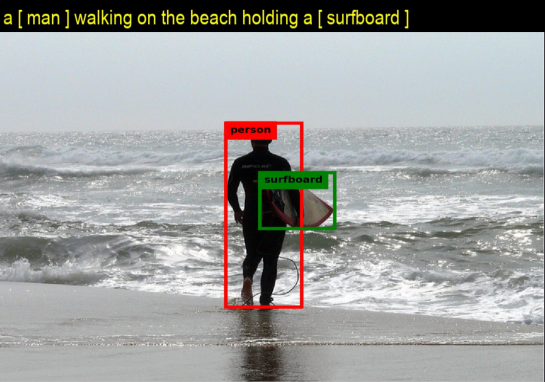
In this work, we improve the previous implementation of a state-of-the-art image captioning model called Neural Baby Talk [1], that ensures the “visual grounding” of the generated words in the caption. Neural Baby Talk is the first deep learning model to generate captions containing words that relate to specific regions in an input image. Fig. 1 explains the visual grounding task. A caption is generated with visual words detected and shown between brackets. Intuitively, it makes sense to ensure the visual grounding of the words in the caption that is being generated by the model. This is because even humans tend to use visual representations of different parts of an image to describe the whole content of an image. In this paper, we show that our twin cascaded attention model, which employs two parallel attention channels, improves the quality of generated captions in comparison with a similar model with one attention channel. We refer to our method as Neural Twins Talk (NTT). Our contributions in this work can be summarized as the following.
-
•
We show that deep learning models deploying attention mechanism [2] on long short-term memory networks (LSTM) [3] could be improved using a novel twin cascaded attention method that we explain in detail in Section III-C. We show this by improving NBT [1] and Bottom-up and Top-down Attention model [4].
-
•
We introduce cascaded adaptive gates. In our model, we use these adaptive gates to improve the performance of the language models in the twin cascaded attention model. The values of adaptive gates are added to each other right before they are applied to the context of each language LSTM. This mechanism ensures that the next language LSTM in our model becomes aware of the attention in the previous language LSTMs.
-
•
We show that by increasing the dropout rate [5] for the second and third language LSTMs in the proposed twin cascaded attention model, we avoid overfitting successfully and we create a refinement effect over the generated captions by creating a meta hypothesis vector. We explain this meta hypothesis and how it is calculated in Section III-C.
-
•
We improve the visual sentinel that was previously used in NBT. We achieve this by performing a non-linear transformation over the context vector coming from the last language LSTM in our model. This is similar to how it is calculated in NBT, except that we use the context vector from the joint LSTM rather than from the first one in our model.
-
•
Instead of modifying the architectural change process while implementing the Neural Twins Talk algorithm, which utilizes parallel neural attention channels, we use an alternative calculation method. We show that the twin cascaded attention model could be utilized over various architectures, only via employing alternative calculation methods. This is further discussed in Section III-D.
The results of our experiments show that a deep model with twin cascaded attention performs better than a deep model with a single channel of attention. At the same time, the results of our experiments show that the twin cascaded attention model performs better than attention models with a single channel of attention in bigger datasets where we have more training data available.
We also perform experiments in MS-COCO with Bottom-up and Top-down Attention model [4], and we show that by employing alternative calculation methods over the same parallel attention channel expansion technique, we could achieve better performance.
Neural architecture search (NAS) techniques have been employed for finding an optimal architecture in a search space of candidate architectures. A good survey of NAS techniques was performed by Elsken et al. [6]. Instead of performing a search in a search space including various architectures, we offer a new search space that includes various calculation methods over the same architecture.
This could indeed lead to a broader search space for NAS techniques. Considering the fact that the primary search space for NAS techniques includes various architectures that are different in design, the secondary search space includes subset of calculation methods for each possible architecture inside the primary search space.
Our focus in this work is on showing the effectiveness of applying Neural Twins Talk model over two different architectures for image captioning. This is done in order to show that not only the Neural Twins Talk model performs better than similar models with one channel of attention, but also to show that employing Neural Twins Talk over various models is achievable via utilizing alternative calculation methods.
II Related Work
The closest related work to our work is NBT [1]. NBT benefits from the improvements brought about by Bottom-up and Top-down Attention model [4] and provides us with information regarding the visual grounding of the generated words in the caption for the input image. In NBT and Bottom-up and Top-down Attention [4], the authors pre-trained Faster-RCNN [7] on COCO [8] with a CNN backbone (Resnet101 [9]) trained on COCO and ImageNet [10] respectively, creating the region proposal network [7]. This mechanism served as the bottom-up attention. On top of this object detector, there was a two layer top-down attention model that included two Long Short Term Memory (LSTM) [3] units. The first LSTM acted as an attention LSTM while the second LSTM unit acted as a language modeling unit to generate the captions for the input image. This integrated mechanism produced an attentive language model that could be trained on embeddings of the input caption and normalized coordinates from input image to generate the captions for unseen images at test time [1, 4].
Template generation, with slot filling [11, 12, 13] was among the first techniques used to solve the problem of automatic image caption generation. Retrieval methods [14, 15, 16] have also been used for generating image captions, these methods retrieve a caption from caption data-base that best describes an image [17]. However, the most successful techniques have used deep learning models end-to-end for image caption generation. Neural Twins Talk that we present in this paper uses a twin cascaded attention model and is an instance of a deep learning model end-to-end used for automatic image caption generation.
Originally introduced by Sutskever et al. [18], the encoder-decoder architecture divides the translation task into two parts. The first portion performs the encoding process; in the context of image captioning, we could call it the feature extraction phase. The second portion of this process is to pass the encoded features into another embedded space that acts as a decoder for generating the output sequence.
Inspired by the encoder-decoder architecture [18], an early work on image captioning using deep learning models by Kiors et al. [19], employed convolutional layers alongside a multi-modal log bilinear LSTM to map visual and textual features in a shared multi-modal space.
Karpathy et al. [20] used a method similar to Kiros et al. [19], but improved the model by modifying the way it generated embeddings for sentences and visual features in multi-modal space by the LSTM unit. “Show and tell”, introduced by Vinyals et al. [21], illustrated the fact that deep learning models could handle the task of image captioning. They used simple CNN models such as AlexNet [22] and VGG [23] for feature extraction and they used an LSTM as a language modeling unit. “Show Attend and Tell” [21] was one of the most interesting deep image captioning models that demonstrated the usefulness of attention mechanisms in the context of image captioning. Irrespective of the sub-architecture used for the encoder and decoder parts of the model, the general idea is that an encoder extracts features and passes them to a decoder for further analysis. Convolutional architectures [22, 23, 9, 24] and attention mechanisms [25, 26, 27] have almost equally contributed to the success of image and video captioning and visual question answering tasks.
Early deep learning methods for image captioning used straightforward convolutional architectures that operate upon the entire image to extract the visual features that is the encoder part of the deep image captioning model [20, 28, 29, 26]. Anderson et al. [4] introduced the Bottom-Up and Top-Down Attention via using object detectors rather than straightforward convolutional networks in deep image captioning models. Their idea was to make the model attend to different regions of the image to find salient objects among proposed regions. They used Faster R-CNN [7], which is a faster implementation of previous work called Fast R-CNN [30].
Faster R-CNN [7] uses a region proposal network in between each convolutional layer. A bounding box with its coordinates is proposed by the region proposal network. At a convolutional layer, the model refines the coordinates of these regions and keeps adding more bounding boxes as it discovers more objects. An interesting characteristic of Faster R-CNN is that it can use various convolutional architectures as backbone for extracting visual features of the input image. Therefore it is able to use any common architecture such as Alex-net [22] or Res-Nets [9] or the VGG model [23].
There are two main paradigms for using deep learning for generating captions from image features. The first paradigm uses the input image as a whole scene for generating captions [20, 21]. The second paradigm is the method of using important regions in the image similar to dense captioning [31] that generates captions for different regions and creates a final caption by combining the generated captions for those regions [17]. Baby Talk [13] was among the most successful slot filling models for image captioning. This work did not benefit from deep learning. Baby Talk [13] produces sentence templates that contain slots that could be filled in with the names of the objects found in the image. The problem with this approach was that the sentences created by this model were not able to show that they were created by a model that is fully aware of how we humans tend to speak most of the time. For this reason, the authors of NBT [1] introduced a novel framework for image captioning that combined the earlier slot filling strategies with deep learning models that were able to handle language modeling. This effective combination served as a foundation for NBT and also for our proposed attention model in this work.
Lu et al. [32] introduced a new attentive language model using a visual sentinel that could attend over different parts of the input image and sentence embeddings. In this work, they proposed the idea of adaptive attention that learned which regions were more important over time by learning the joint relationship between captions from the training set and visual features from region detections. This idea was later used in NBT to create a distinction between visual words and textual words in the caption sentence. Pointer networks [33] were used in NBT in order to let the model adaptively select the important region from the “RoI align layer” [7].
III Methodology
Without modifying the encoder part of the model (bottom-up attention), we only modify the decoder part of NBT (top-down attention) in order to show that twin cascaded attention models are effective in making deep networks deploying LSTMs and attention mechanisms perform better. In order to perform fair comparison, we use the same training details such as the number of epochs and the batch size used for training the models. We use the same object detector results to preserve the network configurations in our experiments. The object detector used in our work was trained on COCO with a ResNet-101 [9] as CNN backbone that was pre-trained on ImageNet [34].
Similar to NBT [1], given the input image, we find the parameters for the network to maximize the likelihood of correct caption for the given image. Given an image sentence pair, while training the model, the goal of the model is to learn which words in the ground truth caption can successfully be grounded into some region in the image. We maximize the likelihood of the correct caption using the summation of the joint probability of the given image and sentence pair.
By applying the chain rule, the joint probability distribution is obtained in terms of a sequence of tokens in the caption generated by the model as the product of the probability of current token and all previously generated tokens in the caption.
A “visual sentinel” is used in NTT, similar to NBT [1], to indicate if the current generated token should be a word describing a region in the image or a word that creates the template sentence. Given this new variable that acts as a default region sentinel, the probability of token given an image and all previously generated tokens is computed. This includes the computation of the joint probability of the visual sentinel and the probability of current token , multiplied by the probability of visual sentinel based on the probability of input image and all previously generated tokens.
III-A Template Generation & Refinement
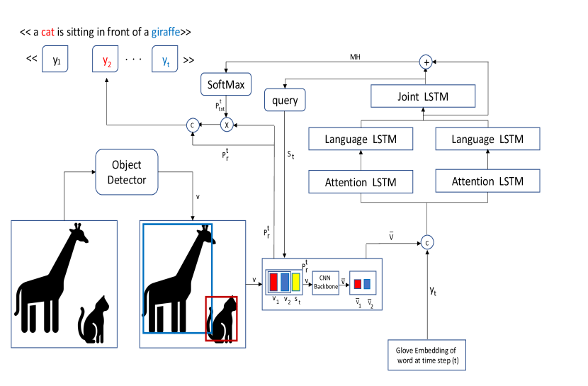
In the NTT model, we employ two channels of attention. This causes the joint LSTM and language LSTMs to become capable of refining the slots in an ensemble manner. We explain this general framework in Fig. 2. At each time step using the default region sentinel, we determine if we need to use the meta hypothesis vector for the textual word that creates the template sentence or if we need to use the pointers for sub-categories and plurality of the word to be placed inside a slot in the template sentence. A Pointer Network [33] is used to create the slots in the template sentence [1]. We modify the way the pointing vector is computed in NBT. We want to make sure the pointing vector is constructed based on the hypothesis vector of the joint LSTM in our model instead of the language LSTM in NBT. At each iteration, we calculate the current hypothesis of an RNN as . At each time step, is the ground truth token while testing, and is the sampled token while training. Consider as the region feature vector for a region of interest. Thus the pointing vector is calculated as the following.
| (1) |
| (2) |
In Eq. 1, and are parameters to be learned by the model and denotes the hypothesis vector of the joint language LSTM that connects the two channels of attention. The visual sentinel in NTT is achieved by applying a gate when the RNN is LSTM [3], as explained in Eq. 3 and Eq. 4.
| (3) |
| (4) |
In Eq. 4, is the context of the joint LSTM at each time step . In Eq. 3, and are weight parameters to be learned and denotes the sigmoid logistic function and is the element-wise product and is the shared LSTM input at time step . By modifying Eq. 2 and infusing the visual sentinel into that equation, we get the probability distribution over the regions in the image as the following.
| (5) |
In Eq. 5, and are parameters and is the probability distribution over the visual sentinel and grounding regions. Next, we feed the meta hypothesis vector into a softmax layer. This is done in order to obtain the probability of textual words regarding the visual features in the image, and all previously generated words, and the visual sentinel as the following.
| (6) |
In Eq. 6, and is the hidden state size of RNN and is the size of the textual vocabulary. In Section III-C, we explain how is calculated. Infusing Eq. 6 and the probability of default region sentinel based on the previous tokens into the probability of textual word in the template sentence based on the default region sentinel generates the probability of generating a word in the template sentence.
Slot filling is performed on the region of interests. The convolutional feature maps pooled from the selected RoI are sent to the attention LSTM; these feature maps are then processed by the attention network before being passed to the language LSTM for template generation and refinement. Using two single layer feed-forward networks with Relu activation function denoted as , we calculate the probability for plurality and fine grained sub-category class as the following.
| (7) |
| (8) |
In Eq. 7 and Eq. 8, U is the vector of embedding of the word for the sub-category that fills the slots, and and are weight parameters to be learned. The last phase of caption template refinement is to consider that is the probability for plurality and that is the probability for the sub-category for the words that are going to fill the slots in the template sentence. Eq. 1 - Eq. 8 are similar to how they are presented in NBT, except that instead of using the hypothesis and context vectors coming from the single language LSTM in NBT, we use the meta hypothesis vector and hypothesis and context vectors coming from the joint LSTM in our model.
III-B Loss Function & Training
We minimize Cross-Entropy loss function, also used in NBT. Regarding visual word extraction, detection model, region feature extraction, previously proposed attentive language model and other implementation details, we encourage the readers to refer to Neural Baby Talk [1].
We train both models on four Nvidia 1080ti GPU cards and we use batch size of 100. We retrain the NBT model and our proposed model (NTT) both from scratch on COCO using the split for this dataset provided by Karpathy [35] and the novel and robust image captioning splits provided by Hendricks et al. [36] and Lu. et al. [1, 34]. In our experiments, we use a consistent beam size of 3.
The difference between our method of training and the original one in NBT is that instead of using a ResNet101 [9] trained on COCO, we use another version of this CNN backbone trained on ImageNet [10] for region feature extraction. We only fine-tune the last layer of the CNN backbone for the region feature extraction phase while training both models. We train both models for 50 epochs with Adam optimizer [37] and we anneal the learning rate every epochs by a factor of . Similar to NBT, we use Glove embeddings [38] for creating word embeddings from the words in the ground truth captions.
III-C Proposed Attention Model
The general framework of NTT was explained in Fig. 2. Inspired by residual learning [9] and multi-head attention [39], we create parallel attention channels and introduce cascaded adaptive gates in our model to employ residual connections between parallel channels. This is why we refer to our proposed decoder as twin cascaded attention decoder.
The shared input of both attention LSTMs in our proposed model is the concatenation of an embedding of token and the set of convolutional features from region proposals . At each time step , the context and hypothesis vectors of the attention LSTM in the first channel of the twin cascaded decoder on the left side are passed to the language LSTM in that channel. Similarly, the context and hypothesis vectors of the attention LSTM in the second channel of the twin cascaded decoder on the right are passed to the language LSTM in that channel. Then, the context vector coming from the language LSTM in the first channel is added to the context vector coming from the language LSTM in the second channel to form the context vector for the joint LSTM. We follow a similar strategy to construct the hypothesis vector for the joint LSTM. This is shown in Fig. 3. We believe this causes the joint LSTM to perform the attention once again, this time, given the context and hypothesis vectors of the first language LSTM on the left side of decoder and the second language LSTM on the right side to learn to perform the attention better.
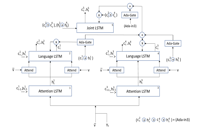
After the hypothesis vectors of the attention LSTMs are computed, they are passed to an attention network. A replica of the attention network is present in each channel. This implies that the first attention network in the top-down channel calculates the attention distribution over set of region features (proposals), and then the second attention network in the same channel calculates the attention distribution over , the set of convolutional features from region proposals.
By adding adaptive gates, and performing the residual learning upon these gates, the attention is successfully passed to lower levels of the decoder. This causes the language LSTMs to work in an ensemble manner. The language LSTMs keep helping one another in generating and refining the template sentences. This happens in a cascaded manner as shown in Fig. 3. At each time step, the language LSTMs in the parallel attention channels receive the hypothesis and context vectors from their lower level attention LSTM in the attention channel they reside in. Similarly, the joint LSTM receives the necessary information from the language LSTMs in each attention channel. This eliminates the need for gathering the information at each time step from the language LSTMs and the joint LSTM, which reduces memory usage. Therefore, the extra memory required by NTT in comparison with NBT, is only around , and most of this increase in memory usage is contributed to feed-forward networks employed in cascaded adaptive gates. We add the context and hypothesis vectors of each language LSTM in the twin attention channels with each other, and we pass it to the joint language LSTM in our model. In a sense, it is a summation of the vectors for all the previous language LSTMs. The attention distribution over set of region features is calculated as explained in Eq. 9.
| (9) |
In Eq. 9, , and are weight parameters to be learned by the model. These parameters are shared between the language LSTMs in the decoder channels. The set of attention values is received by the language LSTM in the attention channel on the left side of the twin cascaded decoder. Similarly, is the set of attention values received by the language LSTM in the attention channel on the right side of the twin cascaded decoder. In total, this attention network is used four times in our model; once for set of region features, and once for , the set of convolutional features from region proposals for the language LSTM in each attention channel.
Next, we show how adaptive gates are calculated in our decoder. Given the input of a language LSTM in an attention channel of our decoder and the hypothesis vector coming form attention LSTM in the same attention channel, we calculate the values for the adaptive gate in that channel. These gates are added to each other in a cascaded manner as shown in Fig. 3. The values for the adaptive gate applied to the joint LSTM are obtained by including the previously cascaded adaptive gates in the attention channels and a mixture of the input of language LSTMs attention channels. This is shown in Eq. 10.
| (10) |
In Eq. 10. , and are the weight parameters for adaptive gates to be found by the model. Each of these adaptive gates are applied to the context vector of their respective language LSTM unit in the decoder. This is shown in Eq. 11. We find that by adding the adaptive gates on each other, the model learns to attend better on different parts of the input for each language LSTM.
| (11) |
The inputs of the final language LSTM in our decoder, which we refer to as the joint language LSTM, are perhaps the most important parts of our decoder. Considering that we have two top-down attention channels, we want another language LSTM that receives the output of both of these channels () with their context vectors () jointly to refine the generated caption one more time. Eq. 12 and Eq. 13 show how the inputs of joint language LSTM is created at each time step.
| (12) |
| (13) |
The final output is calculated based on , and , the hypothesis vectors coming from the last language LSTM in the decoder module as well as the other two language LSTMs in the attention channels. Note that we refer to the concatenation of the hypothesis vector coming from the attention LSTM and the output of the attention networks in each channel as language LSTM input and we show it as . In Eq. 13, denotes the input of language LSTM in the left side channel and denotes the input of language LSTM in the right side channel of the decoder, similarly denotes the input of the joint LSTM that is the result of the element-wise addition between and .
The final output of our model comes from the language LSTMs in attention channels and the joint LSTM in our model. The meta hypothesis is a summation of the output of dropout layers applied to the hypothesis vectors coming form the language LSTMs and joint LSTM. This is done by applying a dropout [5] rate of 0.3 on the output of the language LSTM in the left-side attention channel. Next, we apply a dropout rate of 0.7 on the language LSTM in the second attention channel. Lastly, we apply a dropout rate of 0.8 on the hypothesis vector coming from the joint LSTM that connects the two attention channels with each other. We calculate the summation of the outputs of these dropout layers to create the final hypothesis vector to form the meta hypothesis vector. We show how the meta hypothesis vector is constructed in Eq. 14.
| (14) |
In Eq. 14, denotes the final output of our model, which we refer to as the meta hypothesis vector at time step . We use this vector to generate each word in the caption sentence at time step .
III-D Alternative Calculations
Bottom-up and Top-down attention (Up-Down Attention) model [4], which was published prior to Neural Baby Talk (NBT) [1], was trained on image captioning task without visual grounding. In NBT, for visual grounding we have to deal with template generation and refinement using slot filling. This is done using two attention networks for a language LSTM. One of the attention networks is used for bounding box coordinates and the other one is used for visual features extracted from the bounding boxes. In Up-Down Attention, the model only employs one attention network for the language LSTM in order to calculate the attention values based on visual features and the hypothesis vector coming from the attention LSTM.
We use Eq. 9 in the same way it is defined in Neural Twins Talk utilized over Up-Down Attention. Instead of using new sets of attention weights for bounding box coordinates and visual features as in NTT over NBt, here we only use Eq. 9 once in each attention channel that includes an attention LSTM, an attention network and a language LSTM, in order to perform attention over set of visual features.
In order to show that Neural Twins Talk model can be applied on Up-Down Attention model [4] we employ the same expansion technique that was used for applying Neural Twins Talk on Neural Baby Talk model [1]. To be specific, the proposed attention model in Neural Twins Talk used for enhancing Neural Baby Talk with more attention channels has an architecture identical to the one utilized over Up-Down Attention model.
Instead of modifying the architecture of Neural Twins Talk we modify the way the hypothesis and context vectors are gathered and distributed within LSTM units. The original hypothesis and context gathering in Neural Twins Talk is novel in that instead of gathering the hypothesis and context vectors of LSTM units individually, each language LSTM in each attention channel receives the hypothesis and context vectors from their corresponding lower level attention LSTMs. This is also explained in Fig. 3.
In order to achieve better performance when applying Neural Twins Talk on Up-Down Attention, the hypothesis and context gathering and distribution method is modified. Equations 9 - 14 are identically used in Neural Twins Talk when utilized over Up-Down Attention. Instead of gathering the hypothesis and context vectors for attention LSTMs individually when applying Neural Twins Talk on Neural Baby Talk, here we merge the hypothesis and context vectors coming from the attention LSTMs and the merged hypothesis and context vectors are passed to both attention LSTMs for next iteration step. This is explained in the following equation, note that the LSTMs are assigned with the same numbers as they were in Neural Twins Talk employed for Neural Baby Talk.
| (15) |
Also instead of gathering the hypothesis and context vectors for language LSTMs in each attention channel from their lower level attention LSTMs, we gather the information from the joint LSTM (), which conveys the output hypothesis and context vectors coming from the joint LSTM to the lower level language LSTMs () for next iteration. This is shown in the following equations.
| (16) |
| (17) |
The joint LSTM () receives the merged hypothesis and context vectors coming from language LSTMs () at each time step. This is identical to how the hypothesis and context vectors for the joint LSTM were calculated when Neural Twins Talk was utilized over Neural Baby Talk. This is explained in Eq. 17.
Instead of modifying the dropout rates and how the adaptive gates are calculated, we only modify the way the hypothesis and context vectors are gathered and distributed in a joint manner from the attention LSTMs in the first level of attention channels, and from the joint LSTM and language LSTMs in a circular manner. The inputs of language LSTMs and the joint LSTMs are identical to how they were calculated when Neural Twins Talk was utilized over Neural Baby Talk. This is shown in Eq. 13.
In NTT on NBT model, the joint LSTM, which receives the merged hypothesis and context vectors from the lower level language LSTMs, plays a key role of acting as a bridge between attention channels in this model.
In order to reveal the importance of having a joint LSTM in NTT we follow the modified alternative calculation method and at the same time we remove the joint LSTM and instead we add a third attention channel.
In this modified version of NTT on Up-Down Attention model we want to investigate the tradeoff between removing the joint LSTM and instead adding another parallel attention. The hypothesis and context vectors of all attention LSTMs are merged and fed back to each attention LSTM individually. Similarly, The hypothesis and context vectors of all language LSTMs are merged and fed back to each language LSTM individually without having the joint LSTM. The following equations show how the hypothesis and context vectors are calculated in this version of NTT on Up-down. Note that all attention LSTMs are denoted with odd numbers in Eq. 18 and all language LSTMs are denoted with even numbers in Eq. 19.
| (18) |
| (19) |
In the modified version of NTT on Up-Down Attention model, which was explained above, each attention channel has an attention LSTM followed by a language LSTM. This version of NTT on Up-Down Attention only benefits from a third parallel attention channel in comparison with the first version explained in the beginning of section III-D.
The final meta hypothesis vector that is used as the output of the model is calculated similar to NTT on NBT. The difference here is that the joint LSTM is removed and replaced with the third language LSTM in the third attention channel. For simplicity the third language LSTM was denoted as . Considering this change, the meta hypothesis vector calculation method is identical to the one explained in Eq. 14.
The inputs of language LSTMs for the first language LSTM and second language LSTM are identical to how they were explained in Eq. 13. For the third language LSTM (), similar to the first and second language LSTMs, the input consists of a concatenation of attention values calculated from visual features and the hypothesis vector coming from the corresponding lower level attention LSTM ().
Performing experiments with these two models that follow the alternative calculation method of hypothesis and context gathering, should reveal whether having a joint LSTM with two parallel attentions is more effective for performance gain or having a third parallel channel without a joint LSTM instead. At the same time we could investigate if alternative calculations are effective in performance gain when employed on the same neural expansion algorithm (NTT) over different models such as NBT or Up-Down Attention. The results of experiments with both versions of NTT on Up-Down Attention using alternative calculation methods is discussed in Section IV-B.
IV Discussion & Results
In this section we discuss the results of experiments for Neural Twins Talk applied on Neural Baby Talk [1] in Section IV-A and then we discuss the results of experiments for Neural Twins Talk applied on Bottom-up and Top-down Attention [4] in Section IV-B.
IV-A NTT over NBT
We report the results of our experiments for three different splits on COCO. The first split is provided to us by Karpathy et al. [40]; this split is commonly used for image captioning using deep learning models. The more challenging splits proposed by Hendricks et al. [36] and Lu et al. [1] are Novel and Robust splits.
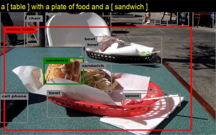
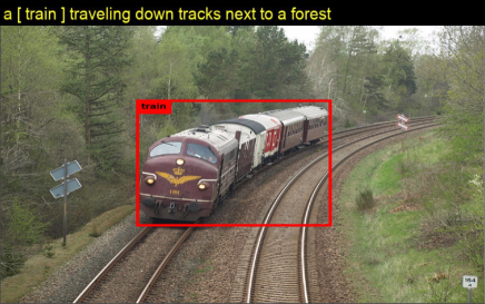
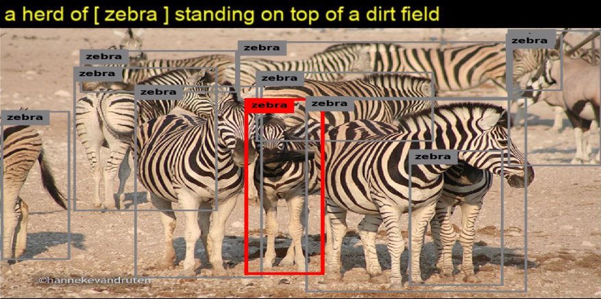
Results for the Karpathy’s split on the COCO dataset are reported in Table I. Instances of images from the validation set of Karpathy’s split and generated captions for them are shown in Fig. 4, Note that in Fig. 4, Fig. 5, and Fig. 6, we are only showing the labels for bounding box detection in images for visualization purposes only. The labels indicate what the object detector thinks about the objects that reside in particular regions of the image. In practice, the captioning models do not use the detection labels. The object detectors are only used to provide us with bounding box coordinates, using another CNN backbone of our choice, we can extract the visual features and feed them to a shared embedded space.
A close look at the results reported in Table I reveals that our model improves the CIDER [8] score by 0.98, which indicates that the model is learning the saliency of the objects that should be mentioned in the captions better than NBT. The improvements on BLEU4 [41] score indicate that the our proposed model is capable of handling long range dependencies between different words of the generated captions better than NBT. On the other hand, the improvement on BLEU1 [41] score reveals that our model is also performing better in word prediction in general. The improvements on SPICE [42] metric indicate that our model is performing better than NBT in describing semantic relationships between the objects in the generated caption. The METEOR metric indicates the quality of the translation task between the ground truth caption and the generated caption for unseen images. Having these metrics gives an overview of how well the models are performing under particular splits on COCO dataset.
| Metrics | |||||
|---|---|---|---|---|---|
| Model | BLEU1 | BLEU4 | CIDER | METEOR | SPICE |
| NBT | 73.84 | 32.64 | 100.71 | 25.79 | 18.92 |
| NTT | 73.93 | 32.92 | 101.69 | 25.8 | 18.99 |
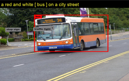
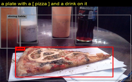
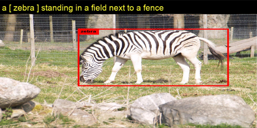
The original Novel split [36] introduced by Hendricks et al. excludes all the captions which contain the name of some particular objects. These names originally were chosen to be “bottle”, “bus”, “couch”, “microwave”, “pizza”, “racket”, “suitcase” and “zebra”. We report the results of our experiments on the Novel split for in-domain images. Table II shows the results for this split. Fig. 5, shows examples of images from the validation set of the Novel split and generated captions for these images. In this split, half of the original COCO validation set images are used for validation randomly, and the rest is used for training.
| Metrics | |||
|---|---|---|---|
| Model | BLEU4 | CIDER | SPICE |
| NBT | 30.79 | 93.83 | 18.17 |
| NTT | 30.82 | 94.01 | 18.26 |
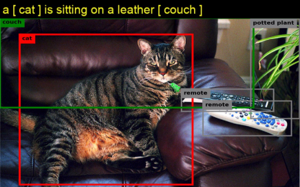
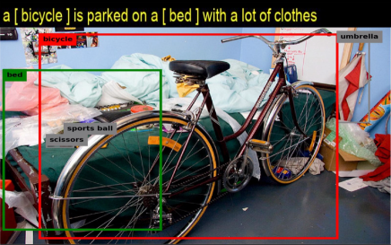
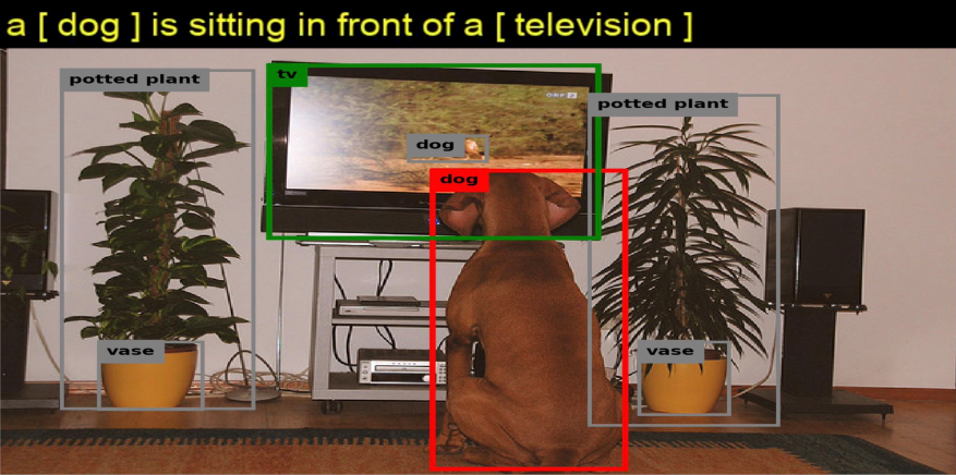
The Robust split was created to evaluate generated captions for novel scene compositions [1]. This split has 110,234 and 3,915 and 9,138 images in train, validation and test portions of this split. The results of our experiments on Robust splits are shown in Table III. Instances of generated captions for the images from the validation set of the Robust split are shown in Fig. 6.
| Metrics | |||
|---|---|---|---|
| Model | BLEU1 | BLEU4 | CIDER |
| NBT | 73.28 | 31.2 | 92.1 |
| NTT | 73.37 | 31.26 | 92.21 |
The overall results over three different splits suggest that twin cascaded attention model in NTT improves the previously implemented attention model in NBT, especially in larger domains. In other words, by looking at the results for Karpathy’s [35], Robust [1] and Novel [36] splits, we observe that the highest amount of improvement on CIDER score is achieved under Karpathy’s split that has a larger amount of training data available. This could indicate over-fitting under the other two splits. We suspect that this over-fitting is caused by the differences in the numbers of training examples under different splits. The results of our experiments suggest that if we employ more cascaded attention channels in deep networks we could achieve better performance, specifically in domains that include more training data.
We improved the results in all metrics for the Karpathy’s split [40] on COCO. We also improved the results in three metrics out of five for Robust and Novel splits. The results of the experiments clearly indicate that twin cascaded attention model could further improve deep networks that employ attention mechanisms with a single channel of attention in domains with sufficient amount of data.
Our proposed method benefits from employing additional attention channels. The results of our experiments suggest that in the near future, with larger amounts of GPU memory, we could employ more attention channels and train such models in bigger domains with larger amount of data to achieve better performance. The results also suggest that a model with a single attention channel could perform better in smaller domains with less amount of data. Therefore, our proposed method is suitable when a particular deep learning model is going to be used in a larger domain.
Our proposed attention model could be considered a flexible structure that could be expanded up to the current GPU memory limits. The key to successfully expanding the proposed cascaded attention model with more attention channels lies in finding the proper dropout rates for the outputs of language LSTMs and the joint LSTMs in the expanded model. We found that increasing the dropout rate for the language LSTMs and the joint LSTM creates a decrementing refinement effect in the proposed cascaded attention model.
IV-B Alternative Calculations
As we explained in Section III-D, we modified the hypothesis and context gathering and distribution in Neural Twins Talk in order to make the model suitable for Up-Down Attention model. The reason is that in our experiments we found that with the original hypothesis and context vectors calculation methods, Neural Twins Talk would achieve slightly lower results under all metrics when applied on Up-Down Attention model. Therefore, by modifying the way the hypothesis and context vectors are calculated, we successfully achieve better performance for Neural Twins Talk applied on Up-Down Attention in comparison with the original Up-Down Attention model that utilizes one channel of attention instead of two channels of attention in Neural Twins Talk.
In this section, first we discuss the results for the NTT utilized over Up-Down attention with alternative calculations, which follows what was explained in Eq. 15 - Eq. 17, and is denoted as NTTUD-v1 in Table IV. Following that we discuss the results for NTT utilized over Up-Down Attention with alternative calculations and having a third parallel attention channel without the joint LSTM following what was explained in Eq. 18 and Eq. 19, which is denoted as NTTUD-v2 in Table IV.
We trained the original Up-Down Attention model [4] and NTTUD-v1 and NTTUD-v2 models all from scratch without any pre-training. The CNN backbone used for all three models explained in Section III-D was pre-trained on ImageNet [10] without fine-tuning. We trained all three models for 30 epochs, and the learning rate and other training details are identical to those used in experiments for NTT over NBT.
| Metrics | |||||
|---|---|---|---|---|---|
| Model | BLEU1 | BLEU4 | CIDER | METEOR | SPICE |
| NTTUD-v1 | 76.51 | 34.49 | 111.24 | 27.49 | 20.62 |
| NTTUD-v2 | 76.13 | 34.01 | 110.51 | 27.28 | 20.39 |
| Up-Down [4] | 76.19 | 34.22 | 110.27 | 27.12 | 20.23 |
The results of experiments in Table IV clearly indicate that NTTUD-v1, which employs NTT over Up-Down Attention employing alternative calculations performs better than NTTUD-v2, which uses a third parallel attention channel without a joint LSTM. The performance improvement in NTTUD-v1 in comparison with NTTUD-v2 shows that having a joint LSTM is necessary for the Neural Twins Talk architecture. At the same time we could observe that adding a third parallel channel without a joint LSTM improves the performance of a similar model with one channel of attention, yet if the model is equipped with a joint LSTM, even with two parallel attention channels performs better. We can also observe that both NTTUD-v1 and NTTUD-v2 are performing better than a similar model with one channel of attention. This shows that adding parallel attention channels improves the performance of a deep learning model with attention and LSTM units. This is what we also observed in experiment results for NTT over NBT.
Another point worthy of being mentioned here is that NTTUD-v1 performs better under all metrics including the BLEU scores in comparison with the Up-Down Attention model, whereas NTTUD-v2 which employs three parallel attention channels without a joint LSTM, performs better under CIDER, SPICE and METEOR, while performing slightly worse under BLEU scores in comparison with Up-Down Attention model. This shows that the joint LSTM is helping the NTT model with learning the sentence structure and grammatical correctness of the image captions generated by the model.
Alternative calculations were clearly shown to be useful in gaining performance boost when NTT over NBT was employed over Up-Down Attention. Instead of changing the architecture of NTT we only modified the way the hypothesis and context vectors are gathered and distributed in NTT over Up-Down Attention (NTTUD-v1). Because the alternative calculations showed their effectiveness in performance gain when NTTUD-v1 was used, we also developed NTTUD-v2 to investigate the importance of having a joint LSTM in NTT.
Alternative calculations of hypothesis and context vectors over the same model with LSTMs and attention leads to better performance. This shows that for every architecture containing LSTMs and attention there could be a subset of alternative calculation methods for hypothesis and context vectors in the model that could further improve the performance of that model.
Considering the effectiveness of alternative calculation methods we could conclude that these methods could potentially create another search space for Neural Architecture Search (NAS) methods where each candidate in the search space of architectures could have a subset of alternative calculation method candidates. If these NAS models perform the search not only in architecture search space but also in alternative calculation methods search space, these models could potentially find a better setting for an architecture where it performs better than the same architecture with conventional calculation methods in deep learning models.
V Conclusions
We introduced a new attention model, namely twin cascaded attention model that employs cascaded adaptive gates and shows the importance of having multiple attention channels rather than having one attention channel in a deep learning model. Looking at the results, we observe that these improvements have led to performance gain, and these results also promise that in the near future, having more GPU memory, we could employ more parallel attention channels to achieve better results. The results also suggest that employing more attention channels demands more training data. In other words, we need more data to train more attention channels. Our proposed method promises advancements and improvements in deep neural networks employing attention mechanisms for image captioning and other similar tasks in vision-language.
References
- [1] Jiasen Lu, Jianwei Yang, Dhruv Batra and Devi Parikh “Neural Baby Talk” In Proceedings of the IEEE Conference on Computer Vision and Pattern Recognition (CVPR), 2018, pp. 7219–7228
- [2] Dzmitry Bahdanau, Kyunghyun Cho and Yoshua Bengio “Neural Machine Translation by Jointly Learning to Align and Translate” In 3rd International Conference on Learning Representations, ICLR 2015, 2015
- [3] Sepp Hochreiter and Jürgen Schmidhuber “Long Short-Term Memory” In Neural Comput. 9.8 Cambridge, MA, USA: MIT Press, 1997, pp. 1735–1780 DOI: 10.1162/neco.1997.9.8.1735
- [4] Peter Anderson et al. “Bottom-Up and Top-Down Attention for Image Captioning and Visual Question Answering” In The IEEE Conference on Computer Vision and Pattern Recognition (CVPR), 2018, pp. 6077–6086
- [5] Nitish Srivastava et al. “Dropout: A Simple Way to Prevent Neural Networks from Overfitting” In Journal of Machine Learning Research 15.56, 2014, pp. 1929–1958
- [6] Thomas Elsken, Jan Hendrik Metzen and Frank Hutter “Neural Architecture Search: A Survey” In Journal of Machine Learning Research 20.55, 2019, pp. 1–21 URL: http://jmlr.org/papers/v20/18-598.html
- [7] Shaoqing Ren, Kaiming He, Ross Girshick and Jian Sun “Faster R-CNN: Towards Real-Time Object Detection with Region Proposal Networks” In Advances in Neural Information Processing Systems 28 Curran Associates, Inc., 2015, pp. 91–99
- [8] Tsung-Yi Lin et al. “Microsoft COCO: Common Objects in Context” In Computer Vision – ECCV 2014 Cham: Springer International Publishing, 2014, pp. 740–755
- [9] K. He, X. Zhang, S. Ren and J. Sun “Deep Residual Learning for Image Recognition” In 2016 IEEE Conference on Computer Vision and Pattern Recognition (CVPR), 2016, pp. 770–778 DOI: 10.1109/CVPR.2016.90
- [10] J. Deng et al. “ImageNet: A large-scale hierarchical image database” In 2009 IEEE Conference on Computer Vision and Pattern Recognition, 2009, pp. 248–255 DOI: 10.1109/CVPR.2009.5206848
- [11] Ali Farhadi et al. “Every Picture Tells a Story: Generating Sentences from Images” In Computer Vision – ECCV 2010 Berlin, Heidelberg: Springer Berlin Heidelberg, 2010, pp. 15–29
- [12] Siming Li et al. “Composing Simple Image Descriptions Using Web-scale N-grams” In Proceedings of the Fifteenth Conference on Computational Natural Language Learning, CoNLL ’11 Portland, Oregon: Association for Computational Linguistics, 2011, pp. 220–228
- [13] G. Kulkarni et al. “BabyTalk: Understanding and Generating Simple Image Descriptions” In IEEE Transactions on Pattern Analysis and Machine Intelligence 35.12, 2013, pp. 2891–2903 DOI: 10.1109/TPAMI.2012.162
- [14] Micah Hodosh, Peter Young and Julia Constanze Hockenmaier “Framing image description as a ranking task: Data, models and evaluation metrics” In IJCAI 2015 - Proceedings of the 24th International Joint Conference on Artificial Intelligence, IJCAI International Joint Conference on Artificial Intelligence International Joint Conferences on Artificial Intelligence, 2015, pp. 4188–4192
- [15] Vicente Ordonez, Girish Kulkarni and Tamara L. Berg “Im2Text: Describing Images Using 1 Million Captioned Photographs” In Advances in Neural Information Processing Systems 24 Curran Associates, Inc., 2011, pp. 1143–1151
- [16] Chen Sun, Chuang Gan and Ram Nevatia “Automatic Concept Discovery From Parallel Text and Visual Corpora” In The IEEE International Conference on Computer Vision (ICCV), 2015, pp. 2596–2604
- [17] MD. Hossain, Ferdous Sohel, Mohd Fairuz Shiratuddin and Hamid Laga “A Comprehensive Survey of Deep Learning for Image Captioning” In ACM Comput. Surv. 51.6 New York, NY, USA: ACM, 2019, pp. 118:1–118:36 DOI: 10.1145/3295748
- [18] Ilya Sutskever, Oriol Vinyals and Quoc V Le “Sequence to Sequence Learning with Neural Networks” In Advances in Neural Information Processing Systems 27 Curran Associates, Inc., 2014, pp. 3104–3112
- [19] Ryan Kiros, Ruslan Salakhutdinov and Rich Zemel “Multimodal Neural Language Models” In Proceedings of the 31st International Conference on Machine Learning 32.2, Proceedings of Machine Learning Research Bejing, China: PMLR, 2014, pp. 595–603
- [20] Andrej Karpathy, Armand Joulin and Li F Fei-Fei “Deep Fragment Embeddings for Bidirectional Image Sentence Mapping” In Advances in Neural Information Processing Systems 27 Curran Associates, Inc., 2014, pp. 1889–1897
- [21] Oriol Vinyals, Alexander Toshev, Samy Bengio and Dumitru Erhan “Show and Tell: A Neural Image Caption Generator” In The IEEE Conference on Computer Vision and Pattern Recognition (CVPR), 2015, pp. 3156–3164
- [22] Alex Krizhevsky, Ilya Sutskever and Geoffrey E Hinton “ImageNet Classification with Deep Convolutional Neural Networks” In Advances in Neural Information Processing Systems 25 Curran Associates, Inc., 2012, pp. 1097–1105
- [23] Karen Simonyan and Andrew Zisserman “Very Deep Convolutional Networks for Large-Scale Image Recognition” In International Conference on Learning Representations, 2015
- [24] Saining Xie et al. “Aggregated Residual Transformations for Deep Neural Networks” In The IEEE Conference on Computer Vision and Pattern Recognition (CVPR), 2017, pp. 1492–1500
- [25] K. Cho, A. Courville and Y. Bengio “Describing Multimedia Content Using Attention-Based Encoder-Decoder Networks” In IEEE Transactions on Multimedia 17.11, 2015, pp. 1875–1886 DOI: 10.1109/TMM.2015.2477044
- [26] Kate Xu “Ask, Attend and Answer: Exploring Question-Guided Spatial Attention for Visual Question Answering” In Computer Vision – ECCV 2016 Cham: Springer International Publishing, 2016, pp. 451–466
- [27] Xu Jia, Efstratios Gavves, Basura Fernando and Tinne Tuytelaars “Guiding the Long-Short Term Memory Model for Image Caption Generation” In The IEEE International Conference on Computer Vision (ICCV), 2015, pp. 2407–2415
- [28] Jeffrey Donahue et al. “Long-Term Recurrent Convolutional Networks for Visual Recognition and Description” In The IEEE Conference on Computer Vision and Pattern Recognition (CVPR), 2015, pp. 2625–2634
- [29] Kelvin Xu et al. “Show, Attend and Tell: Neural Image Caption Generation with Visual Attention” In Proceedings of the 32nd International Conference on Machine Learning 37, Proceedings of Machine Learning Research Lille, France: PMLR, 2015, pp. 2048–2057
- [30] Ross Girshick “Fast R-CNN” In The IEEE International Conference on Computer Vision (ICCV), 2015, pp. 1440–1448
- [31] J. Johnson, A. Karpathy and L. Fei-Fei “DenseCap: Fully Convolutional Localization Networks for Dense Captioning” In 2016 IEEE Conference on Computer Vision and Pattern Recognition (CVPR), 2016, pp. 4565–4574 DOI: 10.1109/CVPR.2016.494
- [32] Jiasen Lu, Caiming Xiong, Devi Parikh and Richard Socher “Knowing When to Look: Adaptive Attention via a Visual Sentinel for Image Captioning” In 2017 IEEE Conference on Computer Vision and Pattern Recognition (CVPR), 2017, pp. 3242–3250
- [33] Oriol Vinyals, Meire Fortunato and Navdeep Jaitly “Pointer Networks” In Advances in Neural Information Processing Systems 28 Curran Associates, Inc., 2015, pp. 2692–2700
- [34] Jianwei Yang, Jiasen Lu, Dhruv Batra and Devi Parikh “Implementation of NeuraBabyTalk available at https://github.com/jiasenlu/NeuralBabyTalk”, 2018 URL: https://github.com/jiasenlu/NeuralBabyTalk
- [35] A. Karpathy and L. Fei-Fei “Deep Visual-Semantic Alignments for Generating Image Descriptions” In IEEE Transactions on Pattern Analysis and Machine Intelligence 39.4, 2017, pp. 664–676 DOI: 10.1109/TPAMI.2016.2598339
- [36] Lisa Anne Hendricks et al. “Deep Compositional Captioning: Describing Novel Object Categories Without Paired Training Data” In The IEEE Conference on Computer Vision and Pattern Recognition (CVPR), 2016, pp. 1–10
- [37] Diederik P. Kingma and Jimmy Ba “Adam: A Method for Stochastic Optimization” In International Conference on Learning Representations (ICLR), 2015
- [38] Jeffrey Pennington, Richard Socher and Christopher D. Manning “GloVe: Global Vectors for Word Representation” In Empirical Methods in Natural Language Processing (EMNLP), 2014, pp. 1532–1543
- [39] Ashish Vaswani et al. “Attention is All you Need” In Advances in Neural Information Processing Systems 30 Curran Associates, Inc., 2017, pp. 5998–6008
- [40] Andrej Karpathy and Li Fei-Fei “Deep visual-semantic alignments for generating image descriptions.” In The IEEE Conference on Computer Vision and Pattern Recognition (CVPR) USA: IEEE Computer Society, 2015, pp. 3128–3137
- [41] Kishore Papineni, Salim Roukos, Todd Ward and Wei-Jing Zhu “Bleu: a Method for Automatic Evaluation of Machine Translation” In Proceedings of the 40th Annual Meeting of the Association for Computational Linguistics Philadelphia, Pennsylvania, USA: Association for Computational Linguistics, 2002, pp. 311–318 DOI: 10.3115/1073083.1073135
- [42] Peter Anderson, Basura Fernando, Mark Johnson and Stephen Gould “SPICE: Semantic Propositional Image Caption Evaluation” In ECCV, 2016, pp. 382–398