Scheduling with Communication Delay in Near-Linear Time

Abstract

We consider the problem of efficiently scheduling jobs with precedence constraints on a set of identical machines in the presence of a uniform communication delay. Such precedence-constrained jobs can be modeled as a directed acyclic graph, $G=(V,E)$. In this setting, if two precedence-constrained jobs $u$ and $v$, with $v$ dependent on $u$ ($u\prec v$), are scheduled on different machines, then $v$ must start at least $\rho$ time units after $u$ completes. The scheduling objective is to minimize makespan, i.e. the total time from when the first job starts to when the last job finishes. The focus of this paper is to provide an efficient approximation algorithm with near-linear running time. We build on the algorithm of Lepere and Rapine [STACS 2002] for this problem to give an $O\left(\frac{\ln\rho}{\ln\ln\rho}\right)$-approximation algorithm that runs in $\tilde{O}(|V|+|E|)$ time.

1 Introduction

The problem of efficiently scheduling a set of jobs over a number of machines is a fundamental optimization problem in computer science that becomes ever more relevant as computational workloads become larger and more complex. Furthermore, in real-world data centers, there exists non-trivial communication delay when data is transferred between different machines. There is a variety of very recent literature devoted to the theoretical study of this topic  [DKR⁺20, DKR⁺21, MRS⁺20]. However, all such literature to date focuses on obtaining algorithms with good approximation factors for the schedule length, but these algorithms require $\omega(n^{2})$ time (and potentially polynomially more) to compute the schedule. In this paper, we instead focus on efficient, near-linear time algorithms for scheduling while maintaining an approximation factor equal to that obtained by the best-known algorithm for our setting [LR02].

Even simplistic formulations of the scheduling problem (e.g. precedence-constrained jobs with unit length to be scheduled on $M$ machines) are typically NP-hard, and there is a rich body of literature on designing good approximation algorithms for the many variations of multiprocessor scheduling (refer to [Bru10] for a comprehensive history of such problems). Motivated by a desire to better understand the computational complexity of scheduling problems and to tackle rapidly growing input sizes, we ask the following research question:

How computationally expensive is it to perform approximately-optimal scheduling?

In this paper, we focus on the classical problem of multiprocessor scheduling with communication delays on identical machines where all jobs have unit size. The jobs that need to be scheduled have data dependencies between them, where the output of one job acts as the input to another. These dependencies are represented using a directed acyclic graph (DAG) $G=(V,E)$ where each vertex $v\in V$ corresponds to a job and an edge $(u,v)\in E$ indicates that job $u$ must be scheduled before $v$. In our multiprocessor environment, if these two jobs are scheduled on different machines, then some additional time must be spent to transfer data between them. We consider the problem with uniform communication delay; in this setting, a uniform delay of $\rho$ is incurred for transferring data between any two machines. Thus for any edge $(u,v)\in E$, if the jobs $u$ and $v$ are scheduled on different machines, then $v$ must be scheduled at least $\rho$ units of time after $u$ finishes. Since the communication delay $\rho$ may be large, it may actually be more efficient for a machine to recompute some jobs rather than wait for the results to be communicated. Such duplication of work can reduce schedule length by up to a logarithmic factor [MRS⁺20] and has been shown to be effective in minimizing latency in schedulers for grid computing and cloud environments [BOC08, CTR⁺17]. Our scheduling objective is to minimize the makespan of the schedule, i.e., the completion time of the last job. In the standard three field notation for scheduling problems, this problem is denoted “$P\mid\textrm{duplication},\textrm{prec},p_{j}=1,c\mid C_{\max}$”, where $c$ indicates uniform communication delay.

This problem was studied by Lepere and Rapine, who devised an $O(\ln\rho{}/\ln\ln\rho{})$-approximation algorithm for it [LR02], under the assumption that the optimal solution takes at least $\rho{}$ time. However, their analysis was primarily concerned with getting a good quality solution and less with optimizing the running time of their polynomial-time algorithm. A naïve implementation of their algorithm takes roughly $O(m{}\rho{}+n{}\ln M{})$ time, where $n$ and $m$ are the numbers of vertices and edges in the DAG, respectively, and $M$ is the number of machines. This runtime is based on two bottlenecks, (i) the computation of ancestor sets, which can be done in $O(m{}\rho{})$ time via propagating in topological order plus merging and (ii) list scheduling, which can be done in $O(n\ln M{})$ time by using a priority queue to look up the least loaded machine when scheduling a set of jobs.

However, with growing input sizes, it is highly desirable to obtain a scheduling algorithm whose running time is linear in the size of the input. Our primary contribution is to design a near-linear time randomized approximation algorithm while preserving the approximation ratio of the Lepere-Rapine algorithm:

Theorem 1.

There is an $O(\ln\rho{}/\ln\ln\rho{})$-approximation algorithm for scheduling jobs with precedence constraints on a set of identical machines in the presence of a uniform communication delay that runs in $O\left(n\ln M+\frac{m\ln^{3}n\ln\rho}{\ln\ln\rho}\right)$ time, with high probability, assuming that the optimal solution has cost at least $\rho$.

Of course, this is tight, up to log factors, because any algorithm for this problem must respect the precedence constraints, which require $\Omega(n+m)$ time to read in. In the settings where our algorithm is more efficient than Lepere-Rapine, the approximation factor of the algorithm is still very small (near-constant in the cases where $\rho=\text{poly}\log n$), yet our algorithm achieves a better runtime while maintaining the same approximation compared to the previous best-known algorithm for the problem.

1.1 Related Work

Algorithms for scheduling problems under different models have been studied for decades, and there is a rich literature on the topic (refer to [Bru10] for a comprehensive look). Here we review work on theoretical aspects of scheduling with communication delay, which is most relevant to our results.

Without duplication, scheduling a DAG of unit-length jobs with unit communication delay was shown to be NP-hard by Rayward-Smith [RS87], who also gave a 3-approximation for this problem. Munier and König gave a $4/3$-approximation for an unbounded number of machines [MK97], and Hanen and Munier gave a $7/3$-approximation for a bounded number of machines [HM01]. Hardness of approximation results were shown in [BGK96, HLV94, Pic95]. In recent results, Kulkarni et al. [KLTY20] gave a quasi-polynomial time approximation scheme for a constant number of machines and a constant communication delay, whereas Davies et al. [DKR⁺20] gave an $O(\log\rho\log M)$ approximation for general delay and number of machines. Even more recently, Davies et al. [DKR⁺21] presented a $O(\log^{4}n)$-approximation algorithm for the problem of minimizing the weighted sum of completion times on related machines in the presence of communication delays. They also obtained a $O(\log^{3}n)$-approximation algorithm under the same model but for the problem of minimizing makespan under communication delay. Notably, none of the aforementioned algorithms consider duplication and the most recent algorithms have running times that are large polynomials.

Allowing the duplication of jobs was first studied by Papadimitriou and Yannakakis [PY90], who obtained a 2-approximation algorithm for scheduling a DAG of identical jobs on an unlimited number of identical machines. A number of papers have improved the results for this setting [AK98, DA98, PLW96]. With a finite number of machines, Munier and Hanen [MH97] proposed a 2-approximation algorithm for the case of unit communication delay, and Munier [Mun99] gave a constant approximation for the case of tree precedence graphs. For a general DAG and a fixed delay $\rho$, Lepere and Rapine [LR02] gave an algorithm that finds a solution of cost $O(\log\rho/\log\log\rho)\cdot(OPT+\rho)$, which is a true approximation if one assumes that $OPT\geq\rho$. This is the main result that our paper builds on. It applies to a set of identical machines and a set of jobs with unit processing times. Recently, an $O(\log M\log\rho/\log\log\rho)$ approximation has been obtained for a more general setting of $M$ machines that run at different speeds and jobs of different lengths by Maiti et al. [MRS⁺20], also under the assumption that $OPT\geq\rho$. However, the running time of this algorithm is a large polynomial ($\omega(n^{2})$), as it requires solving an LP with $\Omega(Mn^{2})$ variables.

Our results so far only apply to scheduling with duplication. In Maiti et al. [MRS⁺20], a polynomial-time reduction is presented that transforms a schedule with duplication into one without duplication (with a polylogarithmic increase in makespan). However, this reduction involves constructing an auxiliary graph of possibly $\Omega(\rho^{2})$ size, and thus does not lend itself easily to a near-linear time algorithm. It would be interesting to see if a near-linear time reduction could be found.

1.2 Technical Contributions

A naïve implementation of the Lepere-Rapine algorithm is bottlenecked by the need to determine the set of all ancestors of a vertex $v$ in the graph, as well as the intersection of this set with a set of already scheduled vertices. Since the ancestor sets may significantly overlap with each other, trying to compute them explicitly (e.g., using DFS to write them down) results in superlinear work. We use a variety of technical ideas to only compute the essential size information that the algorithm needs to make decisions about these ancestor sets.

• Size estimation via sketching. We use streaming techniques to quickly estimate the sizes of all ancestor sets simultaneously. It costs $O((|V|+|E|)\log^{2}n)$ time to make such an estimate once, so we are careful to do so sparingly.

• Work charging argument. Since we cannot compute our size estimates too often, we still need to perform some DFS for ancestor sets. We control the amount of work spent doing so by carefully charging the edges searched to the edges we manage to schedule.

• Sampling and pruning. Because we cannot brute-force search all ancestor sets, we randomly sample vertices, using a consecutive run of unscheduleable vertices as evidence that many vertices are not schedulable. This allows us to pay for an expensive size-estimator computation to prune many ancestor sets simultaneously.

1.3 Organization

The main contribution of this paper is our algorithm for scheduling small subgraphs in near-linear time. We provide a detailed description and analysis of this algorithm in Section 5. Then, we proceed with our algorithm for scheduling general graphs in Section 6.

2 Problem Definition and Preliminaries

An instance of scheduling with communication delay is specified by a directed acyclic graph $G=(V,E)$, a quantity $M\geq 1$ of identical machines, and an integer communication delay $\rho>1$. We assume that time is slotted and let $T=\{1,2,\ldots\}$ denote the set of integer times. Each vertex $v\in V$ corresponds to a job with processing time 1 and a directed edge $(u,v)\in E$ represents the precedence constraint that job $v$ depends on job $u$. In total, there are $n{}=|V|$ vertices (representing jobs) and $m{}=|E|$ precedence constraints. The parameter $\rho{}$ indicates the amount of time required to communicate the result of a job computed on one machine to another. In other words, a job $v$ can be scheduled on a machine at time $t$ only if all jobs $u$ with $(u,v)\in E$ have either completed on the same machine before time $t$ or on another machine before time $t-\rho{}$. We allow for a job to be duplicated, i.e., copies of the same vertex $v\in V$ may be processed on different machines. Let $\mathcal{M}$ be the set of machines available to schedule the jobs. A schedule $\sigma$ is represented by a set of triples $\{(m,v,t)\}\subset\mathcal{M}\times V\times T$ where each triple represents that job $v$ is scheduled on machine $m$ at time $t$. The goal is to obtain a feasible schedule that minimizes the makespan, i.e., the completion time of the last job. Let $\mathsf{OPT}$ denote the makespan of an optimal schedule. Since $\rho{}$ represents the amount of time required to communicate between machines, and in practice, any schedule must communicate the results of the computation, we assume that $\mathsf{OPT}\geq\rho$ as is standard in literature [LR02, MRS⁺20].

Symbol	Meaning
$G=(V,E)$	main input graph
$n=|V|,m{}=|E|$	number of vertices / edges
$H=(V_{H},E_{H})$	subgraph to be scheduled in each phase
$\rho$	communication delay
$u,v$	vertices
$\mathcal{A}_{H}(v)$	set of ancestors of vertex $v$ in graph $H$ including $v$
$\mathcal{A}_{H}(S)$	$\mathcal{A}_{H}(S)=\bigcup_{v\in S}\mathcal{A}_{H}(v)$ in graph $H$
$\mathcal{E}_{H}(v)$ [resp., $\mathcal{E}_{H}(S)]$	edges induced by $\mathcal{A}_{H}(v)$ [resp., $\mathcal{A}_{H}(S)$] in graph $H$
$\hat{a}_{H}(v),\hat{e}_{H}(v)$	estimated size of $\mathcal{A}_{H}(v)$ and $\mathcal{E}_{H}(v)$
$M{}$	number of machines
$\gamma$	threshold for fresh vs. stale vertices

Table 1: Table of Symbols

We now set up some notation to help us better discuss dependencies arising from the precedence constraints of $G$. For any vertex $v\in V$, let $\mathsf{Pred}(v)\triangleq\{u\in V\mid(u,v)\in E\}$ be the set of (immediate) predecessors of $v$ in the graph $G$, and similarly let $\mathsf{Succ}(v)\triangleq\{w\in V\mid(v,w)\in E\}$ be the set of (immediate) successors. For $H=(V_{H},E_{H})$, a subgraph of $G$, we use $\mathcal{A}_{H}(v)\triangleq\{u\in V_{H}\mid\exists\text{ a directed path from $u$ to $v$ in $H$}\}\cup\{v\}$ to denote the set of (indirect) ancestors of $v$, including $v$ itself. Similarly, for $S\subseteq V$, we use $\mathcal{A}_{H}(S)\triangleq\bigcup_{v\in S}\mathcal{A}_{H}(v)$ to denote the indirect ancestors of the entire set $S$. We use $\mathcal{E}_{H}(S)$ to denote the edges of the subgraph induced by $\mathcal{A}_{H}(S)$. We drop the subscript $H$ when the subgraph $H$ is clear from context. Throughout, we use the phrase with high probability to indicate with probability at least $1-\frac{1}{n^{c}}$ for any constant $c\geq 1$.

For convenience, we summarize the notation we use throughout the paper in Table 1.

3 Technical Overview

We start by reviewing the algorithm of Lepere and Rapine [LR02], shown in Algorithm 1, as our algorithm follows a similar outline. Then we describe the technical improvements of our algorithm to achieve near-linear running time.

1 while $G$ is non-empty do

2       Let $H$ be a subgraph of $G$ induced by vertices with at most $\rho+1$ ancestors

3       while $H$ is non-empty do

4             for each vertex $v$ in $H$ do

5                   if greater than $\gamma$ fraction of $\mathcal{A}_{H}(v)$ is unscheduled then

6                         Add $\mathcal{A}_{H}(v)$, in topological order, to a machine with earliest end time

7                  

8            Insert a delay until $C+\rho$ on all machines, where $C$ is the latest end time

9             Remove scheduled vertices from $H$

10      Delete vertices in $H$ from $G$

Algorithm 1 Outline of Lepere Rapine Scheduling Algorithm [LR02]

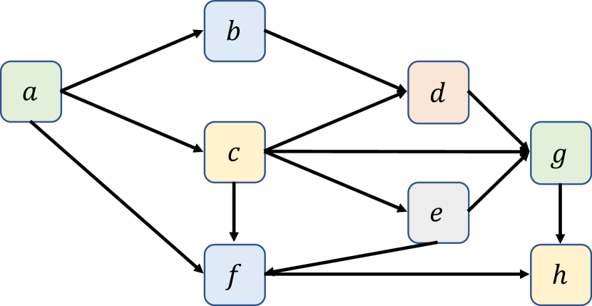
(a) Initial input DAG.

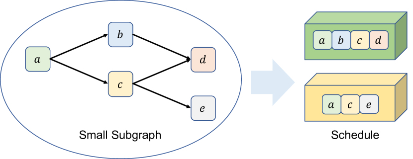
(b) Find a small subgraph in the input graph and schedule the small subgraph.

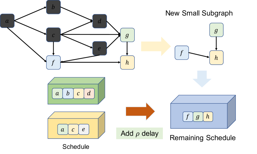
(c) Remove scheduled vertices from the graph. Add a $\rho$ communication delay to the schedule after the previously scheduled jobs. Find a new small subgraph and schedule it.

Figure 1: Overview of the Lepere-Rapine algorithm for scheduling general graphs.

Description of Lepere-Rapine [LR02]. The outer loop (Algorithm 1) iteratively finds small subgraphs of $G$ which consist of vertices that have height at most $\rho+1$. We show in this paper that instead of considering their definition of height, it is sufficient in our algorithm to consider small subgraphs to be those with at most $2\rho$ ancestors. We call one iteration of this loop a phase. Within the phase, $H$ is fully scheduled, after which the algorithm goes on to the next “slice” of $G$. However, $H$ is not scheduled all at once, but instead each iteration of the inner while loop (Algorithm 1) schedules a subset of $H$, which we call a batch. To determine which vertices of $H$ make it into a batch, the algorithm checks the fraction of ancestors of each vertex that have already been scheduled in the same batch. If this fraction for a vertex $v$ is low (we call $v$ fresh in that case), then its ancestor set $\mathcal{A}_{H}(v)$ is list-scheduled as a unit, i.e. ancestor jobs are duplicated, topologically sorted, and placed on one machine. If the fraction of scheduled ancestors is high (in which case we call $v$ stale), $v$ is skipped in this iteration. We skip $v$ to avoid excessive duplication that would create too much load on the machines. After each batch is placed on the machines, a delay of $\rho$ is added to the end of the schedule to allow all the results to propagate. This allows the scheduled jobs to be deleted from $H$. This algorithm is illustrated pictorially in Fig. 1.

Runtime Challenges with Lepere-Rapine. Naively, both finding the small subgraphs as well as determining each batch takes $\Omega(n\rho^{2})$ time. Determining which nodes belong in the current small subgraph is a matter of whether their ancestor counts are more than $\rho$ or at most $\rho$. A standard procedure would be to apply DFS and merge ancestor sets, but that can easily run in $\Omega(\rho^{2})$ time per node (a node may have $\Omega(\rho)$ direct parents, each with an ancestor size of $\Omega(\rho)$ that needs to get merged in).

The other technical hurdle is in determining the batches to schedule. We would like to schedule vertices whose ancestors do not overlap too much. To illustrate the difficulty of applying sketching-based methods (e.g. min-hash), consider the following example. Suppose that $\rho^{2}$ elements have already been scheduled in this batch. Now, we want to find the number of ancestors of vertex $v$, $\mathcal{A}(v)$, that intersect with the currently scheduled batch, where $|\mathcal{A}(v)|\leq\rho$ by construction. By the lower bound given in [PSW14], even estimating (up to $1\pm\epsilon$ relative error with constant probability) the size of this intersection would require sketches of size at least $\varepsilon^{-2}(\rho^{2}/\rho)=\varepsilon^{-2}\rho$. Using such $\rho$-sized sketches over all batches and all small subgraphs require $\Omega(n\rho)$ time in total.

Since $\rho$ may be super-logarithmic, these naive implementations don’t quite meet our goal of a near-linear time algorithm. To summarize, the two main technical challenges for our setting are the following:

Challenge 1.

We must be able to find the small subgraphs in near-linear time.

Challenge 2.

We must be able to find the vertices to add to each batch $B$ in near-linear time.

We solve 1 by relaxing the definition of small subgraph and using count-distinct estimators (discussed in Section 4). The majority of our paper focuses on solving 2 which requires several new techniques for the problem outlined in the rest of this section (Section 3.1 and Section 3.2). The below procedures run on a small subgraph, $H=(V_{H},E_{H})$, where the number of ancestors of each vertex is bounded by $2\rho$. Note the factor of $2$ results from our count-distinct estimator. This is described in Section 5. Our algorithm for scheduling small subgraphs is shown pictorially in Fig. 2.

3.1 Sampling Vertices to Add to the Batch

We first partition the set of unscheduled vertices in $V_{H}$ into buckets based on the estimated number of edges in the subgraph induced by their ancestors. (We place vertex $v$—if it has no ancestors—into the bucket with the smallest index.) We partition by edges instead of vertices because the number of edges in the induced subgraph of the ancestors affects our running time. More formally, let $S_{i}$ be the set of vertices not yet scheduled in iteration $i$ (Algorithm 1, Algorithm 1). We partition $S_{i}$ into $k=O(\log\rho)$ buckets $K_{1},\ldots,K_{k}$ such that bucket $K_{j}$ contains all vertices $w\in S_{i}$ where $\hat{e}(w)\in[2^{j},2^{j+1})$; $\hat{e}(w)$ denotes the estimated number of edges in the subgraph induced by ancestors of $w$.

From each bucket $K_{j}$, in decreasing order of $j$, we sample vertices, sequentially, without replacement. For each sampled vertex $v$, we enumerate its ancestors and determine how many are in the current batch $B$. If at least a $\gamma$-fraction of the vertices are not in $B$ and at least a $\gamma$-fraction of the edges (with both endpoints in $B$) in the induced subgraph $G_{H_{i}}(v)$ are not in $B$, then add $v$ and all its ancestors to $B$. We call such a vertex $v$ fresh. Otherwise, we do not add $v$ to $B$ and label this vertex as stale. For our algorithms, we set $\gamma=\frac{1}{\sqrt{\rho}}$ to minimize the approximation factor but $\gamma$ can be set to any value $\gamma<1/2$. Lepere-Rapine did not consider edges in their algorithm because the number of edges in the induced subgraph does not affect the schedule length; however, considering edges is crucial for our algorithm to run in near-linear time.

For each bucket sequentially, we sample vertices uniformly at random, until we have sampled $O(\log n)$ consecutive vertices that are stale (or we have run out of vertices and the bucket is empty). Then, the key intuition is that for every $v$ that we add to $B$, we can afford to charge the cost of enumerating the ancestor set for $O(\log n)$ additional vertices in the same bucket as well as $O(\log n)$ additional vertices in each bucket with smaller $j$ to it. Because we are looking at buckets with decreasing indices, we can charge the additional vertices found in future buckets to the most recently found fresh vertex. To see why we can charge the samples from buckets with smaller $i$, suppose that one vertex $v$ in bucket $i$ was added to $B$ and no vertices in buckets $(i,\log\rho]$ were added to $B$. Then, the cost charged to $v$ of enumerating the $O(\log n)$ ancestor sets in buckets $[i,\log\rho]$ is at most $\sum_{j=i}^{\log\rho}(2^{\log\rho-j})\log n=O(2^{\log\rho-i}\log n)$, asymptotically the same cost as charging the sampled vertices from bucket $i$.

3.2 Pruning All Stale Vertices from Buckets

After we have performed the sampling procedure, we are still not done. Our goal is to make sure that all vertices which are not included in $B$ are approximately stale. This means that we must remove the stale vertices so that we can perform our sampling procedure again in a smaller sample space in order to find additional fresh vertices. To accomplish this, we perform a pruning procedure involving re-estimating the ancestor sets consisting of vertices that have not been added to the batch. Using these estimates, we remove all stale vertices from our buckets. Note that we do not rebucket the vertices because none of the ancestor sets of the vertices changed sizes. Then, we perform our sampling procedure above (again) to find more fresh vertices. The key is that since we removed all stale vertices, the first sampled vertex from the non-empty bucket with the largest index is fresh.

We perform the above sampling and pruning procedures until each bucket is empty. Then, we schedule the batch and remove all scheduled vertices from $H$ and proceed again with the procedure until the graph is empty. We perform a standard simple greedy list scheduling algorithm (Appendix B) on our batch on $M$ machines.

(a) Input small subgraph.

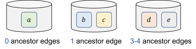
(b) Vertices are bucketed according to the estimate of the number of edges in the induced subgraph of its ancestors.

(c) Vertices are uniformly at random sampled from buckets. Then, vertices which have sufficiently many ancestors and ancestor edges not in $S$ are added to $S$.

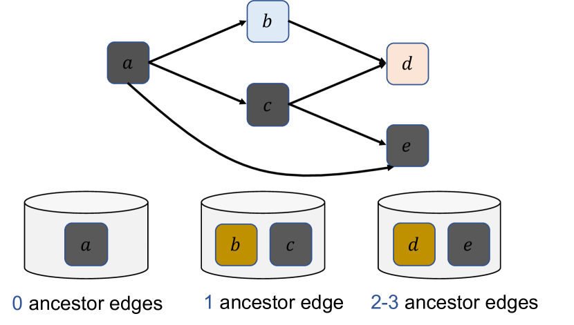
(d) Vertices which are in $S$ or have a large proportion of ancestors or ancestor edges in $S$ are pruned from buckets. $b$ and $d$ are pruned in this example.

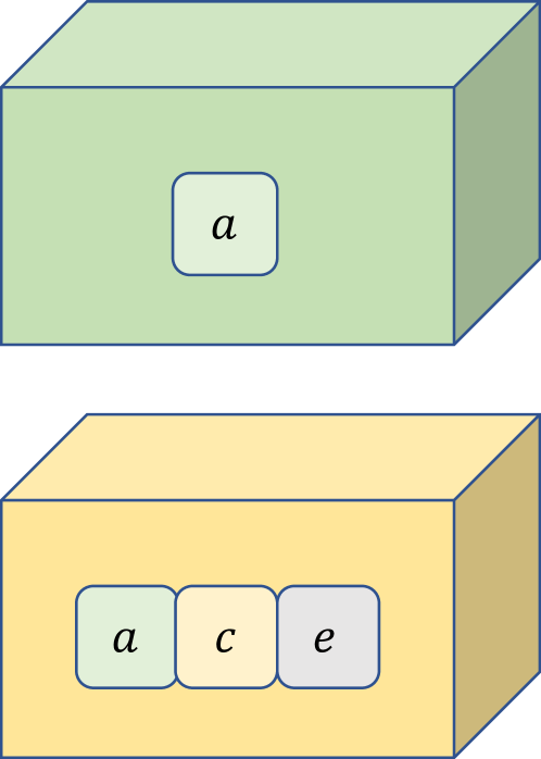
(e) Vertices in $S$ and all ancestors are scheduled by duplicating ancestors and list scheduling.

Figure 2: Overview of our scheduling small subgraphs algorithm. We choose $\gamma=2/3$ here for illustration purposes but in our algorithms $\gamma<1/2$.

4 Estimating Number of Ancestors

Let $\tilde{G}=(\tilde{V},\tilde{E})$ be an arbitrary directed, acyclic graph. We first present our algorithm to estimate the number of ancestors of any vertex $v\in\tilde{V}$. Consider any vertex $v\in\tilde{V}$ and let $p_{1},p_{2},\ldots p_{\ell}$ be the predecessors of $v$ in $\tilde{G}$. Then we have $\mathcal{A}_{\tilde{G}}(v)=\cup_{i=1}^{\ell}\mathcal{A}_{\tilde{G}}(p_{i})\cup\{v\}$ and hence $|\mathcal{A}_{\tilde{G}}(v)|$ is the number of distinct elements in the multiset $\cup_{i=1}^{\ell}\mathcal{A}_{\tilde{G}}(p_{i})\cup\{v\}$. In order to estimate $|\mathcal{A}_{\tilde{G}}(v)|$ efficiently, we use a procedure to estimate the number of distinct elements in a data stream. This problem, known as the count-distinct problem, is well studied and many efficient estimators exist [AMS96, BYJK⁺02, WVZT90, FFGM07, KNW10]. Since we need to estimate $|\mathcal{A}_{\tilde{G}}(v)|$ for all vertices $v\in\tilde{V}$ in near-linear time, we require an additional mergeable property to ensure that we can efficiently obtain an estimate for $|\mathcal{A}_{\tilde{G}}(v)|$ from the estimates of the parent ancestor set sizes $\{|\mathcal{A}_{\tilde{G}}(p_{1})|,\ldots,|\mathcal{A}_{\tilde{G}}(p_{\ell})|\}$.

We formally define the notion of a count-distinct estimator and the mergeable property.

Definition 2.

For any multiset $\mathcal{S}$, let $|\mathcal{S}|$ denote the number of distinct elements in $\mathcal{S}$. We say $T$ is an $(\varepsilon,\delta,D)$-$\mathsf{CountDistinctEstimator}$ for $\mathcal{S}$ if it uses space $D$ and returns a value $\hat{s}$ such that $(1-\varepsilon)|\mathcal{S}|\leq\hat{s}\leq(1+\varepsilon)|\mathcal{S}|$ with probability at least $(1-\delta)$.

Definition 3 (Mergeable Property).

An $(\varepsilon,\delta,D)$-$\mathsf{CountDistinctEstimator}$ exhibits the mergeable property if estimator $T_{1}$ for multiset $\mathcal{S}_{1}$ and estimator $T_{2}$ for multiset $\mathcal{S}_{2}$ can be merged in $O(D)$ time using $O(D)$ space into an $(\varepsilon,\delta,D)$-estimator for $\mathcal{S}_{1}\cup\mathcal{S}_{2}$.

We note that the count-distinct estimator in [BYJK⁺02] satisfies the mergeable property and suffices for our purposes. We include a description of the procedure and a proof of the mergeable property in Appendix A.

Lemma 1 ([BYJK⁺02]).

For any constant $\varepsilon>0$ and $d\geq 1$, there exists an $\left(\varepsilon,\frac{1}{n^{d}},O\left(\frac{1}{\varepsilon^{2}}\log^{2}n\right)\right)$-$\mathsf{CountDistinctEstimator}$ that satisfies the mergeable property where $n$ denotes an upper bound on the number of distinct elements.

Given such an estimator, one can readily estimate the number of ancestors of each vertex $v\in\tilde{V}$ in near-linear time by traversing the vertices of the graph in topological order. An estimator for vertex $v$ can be obtained by merging the estimators for each predecessor of $v$. Similarly, we can also estimate the number of edges $|\mathcal{E}(v)|$ in the subgraph induced by ancestors of any vertex $v$ in near-linear time. We defer a detailed description of these procedures to Algorithm 8 and Algorithm 9 in Appendix A.

Lemma 2.

Given any input graph $\tilde{G}=(\tilde{V},\tilde{E})$ and constants $\varepsilon>0,d\geq 1$, there exists an algorithm that runs in $O\left((|\tilde{V}|+|\tilde{E}|)\log^{2}n\right)$ time and returns estimates $\hat{a}(v)$ and $\hat{e}(v)$ for each $v\in\tilde{V}$ such that $(1-\varepsilon)|\mathcal{A}_{\tilde{G}}(v)|\leq\hat{a}(v)\leq(1+\varepsilon)|\mathcal{A}_{\tilde{G}}(v)|$ and $(1-\varepsilon)|\mathcal{E}_{\tilde{G}}(v)|\leq\hat{e}(v)\leq(1+\varepsilon)|\mathcal{E}_{\tilde{G}}(v)|$ with probability at least $1-\frac{1}{n^{d}}$.

Proof.

Lemma 15 provides us with our desired approximation. Now, all that remains to show is that Algorithm 8 and Algorithm 9 runs within our desired time bounds. Algorithm 8 visits each vertex exactly once. For each vertex, it merges the estimators of each of its immediate predecessors. By Lemma 16, each merge takes $O\left(\frac{1}{\varepsilon^{2}}\log^{2}n\right)$ time. Because we visit each vertex exactly once, we also visit each predecessor edge exactly once. This means that in total we perform $O\left(\frac{m}{\varepsilon^{2}}\log^{2}n\right)$ merges. Since $\varepsilon$ is constant, this algorithm requires $O(m\log^{2}n)$ time. The same proof follows for Algorithm 9. ∎

Throughout the remaining parts of the paper, we assume that $\varepsilon=1/3$ in our estimation procedures and do not explicitly give our results in terms of $\varepsilon$.

5 Scheduling Small Subgraphs in Near-Linear Time

Here, we consider subgraphs $H=(V,E)$ such that every vertex in the graph has a bounded number of ancestors and obtain a schedule for such small subgraphs in near-linear time.

Definition 4.

A small subgraph is a graph $H=(V_{H},E_{H})$ where each vertex $v\in V_{H}$ has at most $2\rho$ ancestors.

Our main algorithm schedules a small graph in batches using Algorithm 3. After scheduling a batch of vertices, we insert a communication delay of $\rho$ time units so that results of the computation from the previous batch are shared with all machines (similar to Lepere-Rapine). Then, we remove all vertices that we scheduled and compute the next batch from the smaller graph. We present this algorithm in Algorithm 2.

Result: A schedule of small subgraph $H$ on $M$ processors.

Input: $H=(V_{H},E_{H})$ where $|\mathcal{A}_{H}(v)|\leq 2\rho$ for all $v\in V_{H}$ and parameter $0<\gamma<1/2$.

1 while $H\neq\varnothing$ do

2       $B\leftarrow$ FindBatch($H,\gamma$). [Algorithm 3]

3       List schedule $\mathcal{A}({v})$ using the $M$ processors for all $v\in B$. (Appendix B)

4       Insert communication delay of $\rho$ time units into the schedule.

5       Remove each $v\in\mathcal{A}(B)$ and all edges adjacent to $v$ from $H$.

6      

7 end while

Algorithm 2 ScheduleSmallSubgraph$(H,\gamma)$

Our algorithm for scheduling small subgraphs relies on two key building blocks – estimating the sizes of the ancestor sets (and ancestor edges) of each vertex (Section 4), and using these estimates to find a batch of vertices that can be scheduled without any communication (possibly by duplicating some vertices). We show how to find a batch in Section 5.1.

5.1 Batching Algorithm

Recall that the plan is for our algorithm to schedule a small subgraph by successively scheduling maximal subsets of vertices in the graph whose ancestors do not overlap too much; we call such a set of vertices a batch. After scheduling each batch, we remove all the scheduled vertices from the graph and iterate on the remaining subgraph.

A detailed description of this procedure is given in Algorithm 3. For each vertex $v\in V_{H}$, let $\hat{a}(v)$ and $\hat{e}(v)$ denote the estimated sizes of $\mathcal{A}_{H}(v)$ and $\mathcal{E}_{H}(v)$ respectively (henceforth referred to as $\mathcal{A}(v)$ and $\mathcal{E}(v)$). Then the $i$-th bucket, $K_{i}$, is defined as $K_{i}=\{v\in V_{H}\mid 2^{i}\leq\hat{e}(v)<2^{i+1}\}$. Since every node $v\in V_{H}$ has at most $O(\rho)$ ancestors, there are only $k=O(\log\rho)$ such buckets. Recall that from Lemma 2, this estimation can be performed in near-linear time. The algorithm maintains a batch $B$ of vertices that is initially empty. For each non-empty bucket $K_{i}$ (processed in decreasing order of size), we repeatedly sample nodes uniformly at random from the bucket (without replacement).

For each sampled node $v\in K_{i}$, we explicitly enumerate the ancestor sets $\mathcal{A}(v)$ and $\mathcal{E}({v})$ and also compute $\mathcal{A}(v)\setminus\mathcal{A}(B)$ and $\mathcal{E}({v})\setminus\mathcal{E}({B})$. Since we can maintain the ancestor sets of the current batch $B$ in a hash table, this enumeration takes $O(|\mathcal{E}({v})|)$ time. A sampled node $v$ is said to be fresh if $|\mathcal{A}(v)\setminus\mathcal{A}(B)|>\gamma|\mathcal{A}(v)|$ and $|\mathcal{E}({v})\setminus\mathcal{E}({B})|>\gamma|\mathcal{E}({v})|$; and said to be stale otherwise. The algorithm adds all fresh nodes to the batch $B$ and continues sampling from the bucket until it samples $\Theta(\log n)$ consecutive stale nodes. Once all the buckets have been processed, we prune the buckets to remove all stale nodes and then repeat the sampling procedure until all buckets are empty.

A bucket $K_{i}$ is reduced when 1) a vertex, $v$, in it is added to $B$, 2) a sampled vertex $v$ is stale and 3) during the pruning process. No vertex remains unscheduled because either a vertex $v$ is scheduled in the current batch or it is stale. For all stale vertices, in Algorithm 2, we remove all the scheduled ancestors of these stale vertices (so the vertices become fresh again). We repeat the procedure given in Algorithm 3 (Algorithm 2 of Algorithm 2) until the entire graph is scheduled (Algorithm 2 of Algorithm 2) so that all vertices are eventually scheduled. The pruning procedure is presented in Algorithm 4. In this step, we again estimate the sizes of ancestor sets of all vertices in the graph $H\setminus\mathcal{A}({B})$ to determine whether a vertex is stale.

Result: Returns batch $B$, the batch of vertices to schedule.

Input: A subgraph $H=(V_{H},E_{H})$ such that $|\mathcal{A}_{H}(v)|\leq 2\rho$ for all $v\in V_{H}$; $0<\gamma<1/2$.

1 Let $N=\Theta(\log n)$.

2 Initially, $B\leftarrow\varnothing$ and all nodes are unmarked.

3 Obtain estimates $\hat{a}(v)$ and $\hat{e}(v)$ for all $v\in V_{H}$.

4 Let bucket $K_{i}=\{v\in V_{H}:2^{i}\leq\hat{e}(v)<2^{i+1}\}$.

5 while at least one bucket is non-empty do

6       for $i=k\text{ to }1$ do

7             Let $s=0$.

8             while $s<N$ and $|K_{i}|>0$ do

9                   Let $v$ be a uniformly sampled node in bucket $K_{i}$.

10                   Find $\mathcal{A}({v})$ and $\mathcal{A}({v})\setminus\mathcal{A}({B})$ as well as $\mathcal{E}({v})$ and $\mathcal{E}({v})\setminus\mathcal{E}({B})$.

11                   if  $|\mathcal{A}({v})\setminus\mathcal{A}({B})|>\gamma|\mathcal{A}({v})|$ and $|\mathcal{E}({v})\setminus\mathcal{E}({B})|>\gamma|\mathcal{E}({v})|$  then

12                         Mark $v$ as fresh, add $v$ and its ancestors to $B$.

13                         Set $s=0$.

14                        

15                  else

16                         Mark $v$ as stale. $s=s+1$.

17                        

18                  Remove $v$ from $K_{i}$.

19                  

20            

21      $K_{1},\ldots,K_{k}\leftarrow$ Prune($H$, $B$, $K_{1}$, …, $K_{k}$) [Algorithm 4].

22Return $B$.

Algorithm 3 FindBatch($H,\gamma$)

Result: New buckets $K_{1},\ldots,K_{k}$.

Input: A graph $H=(V,E)$, a batch $B\subseteq V$, and buckets $K_{1},\ldots,K_{k}$.

1 Obtain estimates $\hat{a}_{H}(v)$ and $\hat{e}_{H}(v)$ for all nodes $v\in\cup_{i=1}^{k}K_{i}$ in the graph $H$.

2 Let $H^{\prime}\leftarrow H\setminus\mathcal{A}({B})$

3 Obtain estimates $\hat{a}_{H^{\prime}}(v)$ and $\hat{e}_{H^{\prime}}(v)$ for all nodes $v\in\cup_{i=1}^{k}K_{i}$ in the graph $H^{\prime}$.

4 for $i=k$ to 1 do

5       for each node $v$ in bucket $K_{i}$ do

6             $X\leftarrow\dfrac{\hat{a}_{H^{\prime}}(v)}{\hat{a}_{H}(v)}$.

7             $Y\leftarrow\dfrac{\hat{e}_{H^{\prime}}(v)}{\hat{e}_{H}(v)}$.

8             if $X\leq 2\gamma$ or $Y\leq 2\gamma$ then

9                   Remove $v$ from $K_{i}$.

10                  

11            

12      

Return the new buckets $K_{1},\ldots,K_{k}$.

Algorithm 4 Prune$(H,B,K_{1},\ldots,K_{k})$

5.2 Analysis

We first provide two key properties of the batch $B$ of vertices found by Algorithm 3 that are crucial for our final approximation factor and then analyze the running time of the algorithm.

5.2.1 Quality of the Schedule

We show that $B$ comprises of vertices whose ancestor sets do not overlap significantly, and further that it is the “maximal” such set.

Lemma 3.

The batch $B$ returned by Algorithm 3 satisfies $|\mathcal{A}(B)|>\gamma\sum_{v\in B}|\mathcal{A}(v)|$ and $|\mathcal{E}(B)|>\gamma\sum_{v\in B}|\mathcal{E}(v)|$.

Proof.

Let $B^{(\ell)}\subseteq B$ denote the set containing the first $\ell$ vertices added to $B$ by the algorithm. We prove the lemma via induction. In the base case, $B^{(1)}$ consists of a single vertex and trivially satisfies the claim. Now suppose that the claim is true for some $\ell\geq 1$ and let $v$ be the $(\ell+1)$-th vertex to be added to $B$. By Algorithm 3 of Algorithm 3, we add a vertex $v$ into $B^{(\ell)}$ if and only if $|\mathcal{A}(v)\setminus\mathcal{A}(B^{(\ell)})|>\gamma|\mathcal{A}(v)|$ and $|\mathcal{E}(v)\setminus\mathcal{E}(B^{(\ell)})|>\gamma|\mathcal{E}(v)|$. Furthermore, since we enumerate $\mathcal{A}(v)$ via DFS, our calculation of the cardinality of each of these sets is exact. We now have, $|\mathcal{A}(B^{(\ell+1)})|=|\mathcal{A}(B^{(\ell)})|+|\mathcal{A}(v)\setminus\mathcal{A}(B)|>|\mathcal{A}(B^{(\ell)})|+\gamma|\mathcal{A}(v)|$. By the induction hypothesis, we now have $|\mathcal{A}(B^{(\ell+1)})|>\gamma\sum_{w\in B^{(\ell)}}\mathcal{A}(w)+\gamma\mathcal{A}(v)=\gamma\sum_{w\in B^{(\ell+1)}}\mathcal{A}(w)$. The same proof also holds for $\mathcal{E}(B)$ and the lemma follows. ∎

Lemma 4.

If a vertex $w$ was not added to $B$, it is pruned by Algorithm 4, with high probability. If a vertex $v$ is pruned by Algorithm 4, then $|\mathcal{A}(v)\setminus\mathcal{A}(B)|\leq 4\gamma|\mathcal{A}(v)|$ or $|\mathcal{E}(v)\setminus\mathcal{E}(B)|\leq 4\gamma|\mathcal{E}(v)|$, with high probability.

Proof.

We first prove that any vertex $v$ that is not added to $B$ must be removed from its bucket by Algorithm 4. Any vertex not added to $B$ must have $|\mathcal{A}(v)\setminus\mathcal{A}(B)|\leq\gamma|\mathcal{A}(v)|$. By Lemma 2, $\hat{a}_{H^{\prime}}(v)\leq 4/3|\mathcal{A}(v)\setminus\mathcal{A}(B)|$ and $\hat{a}_{H}(v)\geq 2/3|\mathcal{A}(v)|$, with high probability. This must mean that $\frac{\hat{a}_{H^{\prime}}(v)}{\hat{a}_{H}(v)}\leq\frac{4/3|\mathcal{A}(v)\setminus\mathcal{A}(B)|}{2/3|\mathcal{A}(v)|}\leq\frac{4/3\gamma|\mathcal{A}(v)|}{2/3|\mathcal{A}(v)|}\leq 2\gamma$. Thus, $v$ will be pruned. The same proof holds for $\hat{e}_{H^{\prime}}(v)$.

We now prove that the pruning procedure successfully prunes vertices with not too many unique ancestors. In Algorithm 4, by Lemma 2 (setting $\epsilon=1/3$), we have with high probability, $\hat{a}_{H^{\prime}}(v)\geq 2/3|\mathcal{A}_{H^{\prime}}(v)|$. Similarly, with high probability, $\hat{a}_{H}(v)\leq 4/3|\mathcal{A}_{H}(v)|$. This means $X=\frac{\hat{a}_{H^{\prime}}(v)}{\hat{a}_{H}(v)}\geq\frac{2/3|\mathcal{A}_{H^{\prime}}(v)|}{4/3|\mathcal{A}_{H}(v)|}=\frac{1}{2}\left(\frac{|\mathcal{A}_{H^{\prime}}(v)|}{|\mathcal{A}_{H}(v)|}\right)$. By the same argument, we also have $Y=\frac{\hat{e}_{H^{\prime}}(v)}{\hat{e}_{H}(v)}\geq\frac{1}{2}\left(\frac{|\mathcal{E}_{H^{\prime}}(v)|}{|\mathcal{E}_{H}(v)|}\right)$ with high probability.

By Algorithm 4 of Algorithm 4, when we remove a vertex $v$ we have either $X\leq 2\gamma$ or $Y\leq 2\gamma$. By the above, $X,Y\geq\frac{1}{2}(4\gamma)=2\gamma$. Thus, the largest that $\left(\frac{|\mathcal{A}_{H^{\prime}}(v)|}{|\mathcal{A}_{H}(v)|}\right)$ or $\left(\frac{|\mathcal{E}_{H^{\prime}}(v)|}{|\mathcal{E}_{H}(v)|}\right)$ can be while still being pruned is $4\gamma$. Thus, with high probability, we have either $\frac{|\mathcal{A}_{H^{\prime}}(v)|}{|\mathcal{A}_{H}(v)|}\leq 4\gamma$ or $\frac{|\mathcal{E}_{H^{\prime}}(v)|}{|\mathcal{E}_{H}(v)|}\leq 4\gamma$. Since $\mathcal{A}_{H^{\prime}}(v)=\mathcal{A}(v)\setminus\mathcal{A}(B)$, the claim follows. ∎

The above two lemmas tell us that there are enough unique elements in each batch $B$, any vertex not added to $B$ will be pruned w.h.p., and the pruning procedure only prunes vertices with a large enough overlap with $B$ w.h.p. This allows us to show the following lemma on the length of the schedule produced by Algorithm 2 for small subgraph $H$. We first show that we only call Algorithm 3 at most $O\left(\log_{1/\gamma}(\rho)\right)$ times from Algorithm 2 of Algorithm 2.

Lemma 5.

The number of batches needed to be scheduled before all vertices in $H$ are scheduled is at most $4\log_{1/4\gamma}(2\rho)$, with high probability.

Proof.

By Lemma 4, each vertex $v$ we do not schedule in a batch $B$ has at least $(1-4\gamma)|\mathcal{A}(v)|$ vertices in $\mathcal{A}(B)$ or at least $(1-4\gamma)|\mathcal{E}(v)|$ edges in $\mathcal{E}(B)$. Since we assumed that all vertices in $H$ have $\leq 2\rho$ ancestors, this means that $v$ can only remain unscheduled for at most $2\log_{1/4\gamma}(4\rho^{2})$ batches until $\mathcal{A}(v)$ and $\mathcal{E}(v)$ both become empty ($G_{v}$ can have at most $4\rho^{2}$ edges). ∎

Using Lemma 5, we can prove the length of the schedule for $H$ using Algorithm 2. The proof of this lemma is similar to the proof of schedule length of small subgraphs in [LR02].

Lemma 6.

With high probability, the schedule obtained from Algorithm 2 has size at most $\frac{|V_{H}|}{\gamma M}+12\rho\log_{1/4\gamma}(2\rho)$ on $M$ processors.

Proof.

By definition of the input, each $\mathcal{A}(v)$ for $v\in V_{H}$ has at most $2\rho$ elements. Recall that we schedule all elements in each batch $B$ by duplicating the common shared ancestors such that we obtain a set of independent ancestor sets to schedule. Then, we use a standard list scheduling algorithm to schedule these lists; see Appendix B for a classic list scheduling algorithm. Each vertex in $H$ gets scheduled in exactly one batch since we remove all scheduled vertices from the subgraph used to compute the next batch. Let $B_{1},B_{2},\ldots,B_{k}$ denote the batches scheduled by Algorithm 2. Let $H_{i}$ be the subgraph obtained from $H$ by removing batches $B_{0},\dots,B_{i-1}$ and adjacent edges. ($B_{0}$ is empty.) By Lemma 3, with high probability, for each batch $B_{i}$, we have $\sum_{v\in B_{i}}|\mathcal{A}_{H_{i}}(v)|\leq\frac{1}{\gamma}|\mathcal{A}_{H_{i}}(B_{i})|$. Let $Z_{i}=\frac{1}{\gamma}|\mathcal{A}_{H_{i}}(B_{i})|$.

Graham’s list scheduling algorithm [Gra69] for independent jobs is known to produce a schedule whose length is at most the total length of jobs divided by the number of machines, plus the length of the longest job. In our case, we treat each ancestor set as one big independent job, and thus for each batch $B_{i}$, this bound becomes $Z_{i}/M+2\rho$.

Finally Algorithm 2 inserts an idle time of $\rho$ between two successive batches. The total length of the schedule is thus upper bounded by (where $k$ is the number of batches):

$$\sum_{i=1}^{k}\left(\frac{Z_{i}}{M}+2\rho+\rho\right) \leq 3\rho\cdot 4\log_{1/4\gamma}(2\rho)\sum_{i=1}^{k}\frac{Z_{i}}{M}\;\;\;\text{(by~{}\lx@cref{creftype~refnum}{lem:round-till-empty})}$$

$$\leq 3\rho\cdot 4\log_{1/4\gamma}(2\rho)+\frac{1}{\gamma M}\cdot\sum_{i=1}^{k}|\mathcal{A}_{H_{i}}(B_{i})|$$

$$=\frac{|V_{H}|}{\gamma M}+12\rho\log_{1/4\gamma}(2\rho)\qed$$

5.2.2 Runtime of Scheduling Small Subgraphs

In order to analyze the running time of Algorithm 3, we need a couple of technical lemmas. The key observation is that although computing the ancestor sets $\mathcal{A}({v})$ and $\mathcal{E}({v})$ (in Algorithm 3) of a vertex $v$ takes $O(|\mathcal{E}({v})|)$ time in the worst case, we can bound the total amount of time spent computing these ancestor sets by the size of the ancestor sets scheduled in the batch. There are two main components to the analysis. First, we show that after every iteration of the pruning step, the number of vertices in each bucket reduces by at least a constant fraction and hence the sampling procedure is repeated at most $O(\ln n)$ times per batch. Secondly, we use a charging argument to upper bound the amount of time spent enumerating the ancestor sets of sampled vertices.

Finding Stale Vertices. We first argue that with high probability, there are at most $O(\ln n)$ iterations of the while loop in Algorithm 3 of Algorithm 3. Intuitively, in each iteration of the while loop, the number of vertices in any bucket $K_{i}$ reduces by at least a constant fraction.

Lemma 7.

For any constant $d\geq 1$ and $\psi>0$, there is a constant $c\geq 1$ such that, with probability at least $1-\frac{1}{n^{d}}$, at most a $\psi$-fraction of remaining nodes in each bucket are fresh after sampling $c\ln n$ stale vertices consecutively.

Proof.

The main approach behind the proof is that we show that for any bucket where a constant fraction $\psi$ of the vertices in the bucket are fresh, for any $c\ln n$ consecutively sampled vertices, we expect to see $\psi c\ln n$ fresh vertices. Furthermore, we show a concentration bound around this expected number of vertices using the Chernoff bound. Thus, we can conclude that if we see $c\ln n$ stale vertices consecutively (with no good vertices), then with high probability, at most a small constant fraction of the remaining nodes in the bucket is fresh.

Algorithm 3 samples the vertices in each bucket $K_{i}$ consecutively, uniformly at random without replacement, until a new fresh vertex is found or at least $c\ln n$ stale vertices are sampled consecutively. Let $F$ be the set of fresh and stale vertices sampled (and removed) so far from bucket $K_{i}$ up to the most recent time a fresh vertex was sampled from $K_{i}$ (i.e. $F$ includes all vertices sampled including and up to the most recent fresh vertex sampled from $K_{i}$). Let $\psi$ be some fraction $0<\psi<1$. Suppose at most a $\psi$-fraction of the vertices in bucket $K_{i}$ are fresh after removing the previously sampled $F$ vertices. Such an $\psi$ exists for every bucket with at least one fresh vertex and one stale vertex after doing such removals. (In the case when all vertices in the bucket are fresh, all vertices from that bucket will be sampled and added to $B$. If all vertices in the bucket are stale, then $c\ln n$ stale vertices will be sampled immediately.)

From here on out, we assume the bucket $K_{i}$ only contains the remaining vertices after the previously sampled $F$ vertices were removed. We assume the number of remaining vertices in $K_{i}$ is more than $c\ln n$. The probability that each of the next sampled vertices is a fresh vertex is at least $\psi$. The expected number of fresh vertices in the $c\ln n$ samples from $K_{i}$ is lower bounded by:

$$\sum_{i=1}^{c\ln n}\left(i\cdot{c\ln n\choose i}\psi^{i}(1-\psi)^{c\ln n-i}\right)=\psi c\ln n.$$

Suppose for our analysis that we only remove stale vertices when we sample them (and not fresh vertices). The above is a lower bound, in this setting, on the expected number of sampled fresh vertices from $K_{i}$ since $\psi$ is the fraction of fresh vertices after removing $F$; if we remove more stale vertices, the fraction of fresh vertices cannot decrease so $\psi$ upper bounds the fraction of fresh vertices in $K_{i}$ as we remove more stale vertices. This assumption is the same as our algorithm when all $c\ln n$ sampled vertices are stale.

By the Chernoff bound, the probability that we sample less than $(1-\varepsilon)\psi c\ln n$ fresh vertices is less than $\exp\left(-\frac{\varepsilon^{2}\psi c\ln n}{2}\right)$. When $c>\frac{1}{(1-\varepsilon)\psi}$, $(1-\varepsilon)\psi c\ln n\geq 1$ for any $0<\varepsilon<1$ and $0<\psi<1$. Then, the probability that no fresh vertices are sampled is less than $\exp\left(-\frac{\varepsilon^{2}\psi c\ln n}{2}\right)=n^{\frac{-\varepsilon^{2}\psi c}{2}}$. It is easy to consider the case for constant $\psi\in(0,1)$. If $\psi=o(1)$, then there exists a constant $\phi$ for which at most a $\phi$-fraction of the vertices in $K_{i}$ are fresh. If $\psi=\omega(1)$, then the probability becomes super-polynomially small. We can sample $c\ln n$ vertices for large enough constant $c\geq\frac{6d}{\varepsilon^{2}\psi}$ such that with probability at least $1-\frac{1}{n^{d}}$ for any constant $d\geq 1$, there exists less than $\psi$-fraction of vertices in the bucket that are fresh if the next $c\ln n$ sampled vertices are stale. The factor of $6$ in the bound $c\geq\frac{6d}{\varepsilon^{2}\psi}$ is useful when we take the union bound over multiple trials (at most $O(n^{2})$) for all buckets used during the course of this algorithm. ∎

Lemma 8.

We perform $O(\ln n)$ iterations of sampling and pruning, with high probability, before all buckets are empty. In other words, with high probability, Algorithm 3 of Algorithm 3 runs for $O(\ln n)$ iterations.

Proof.

We prove the lemma for one bucket $K_{i}$ and by the union bound, the lemma holds for all buckets. First, any sampled vertex which is fresh is added to $B$. Furthermore, we showed in Lemma 4 that any vertex which is stale is removed from $K_{i}$ by Algorithm 4. Since the estimates $\hat{a}(v)$ and $\hat{e}(v)$ are within a $\frac{1}{3}$-factor of $|\mathcal{A}(v)|$ and $|\mathcal{E}(v)|$, respectively, we can upper bound $\frac{\hat{a}_{H^{\prime}}(v)}{\hat{a}_{H}(v)}\leq 2\cdot\frac{|\mathcal{A}(v)\setminus\mathcal{A}(B)|}{|\mathcal{A}(v)|}$ (same holds for $\hat{e}(v)$). If a vertex $v$ is stale, then with high probability, we have either $\frac{\hat{a}_{H^{\prime}}(v)}{\hat{a}_{H}(v)}\leq\frac{2|\mathcal{A}(v)\setminus\mathcal{A}(B)|}{|\mathcal{A}(v)|}\leq 2\gamma$ or $\frac{\hat{e}_{H^{\prime}}(v)}{\hat{e}_{H}(v)}\leq 2\gamma$, and it is removed by Algorithm 4 of Algorithm 4. Since any fresh vertices that are sampled gets added into $B$ and all stale vertices are pruned at the end of each iteration, it only remains to show a large enough number of stale vertices are pruned.

Lemma 7 guarantees that, with high probability, at least $(1-\psi)$-fraction of the vertices in $K_{i}$ are stale for any constant $\psi\in(0,1)$. Then, Algorithm 4 removes at least $(1-\psi)|K_{i}|$ vertices in $K_{i}$ in each iteration. The number of iterations needed is then $\log_{1/(1-\psi)}(|K_{i}|)=O(\ln n)$.

Since there exists $O(\log\rho)$ buckets and $O(m)$ estimates, we can take the union bound on the probability of success over all buckets and estimates. We obtain, with high probability, $O(\log n)$ iterations are necessary before all buckets are empty. ∎

Charging the Cost of Examining Stale Sets. Here we describe our charging argument that allows us to explictly enumerate the ancestor set of each sampled vertex. Computing the ancestor set of a vertex $v$ takes time $O(|\mathcal{E}(v)|)$ using DFS. Since a fresh vertex gets added to the batch, the cost of computing the ancestor set of a fresh vertex can be easily bounded by the set of edges in $\mathcal{E}(B)$, achieving a total cost, specifically, of $O\left(\frac{1}{\gamma}|\mathcal{E}(B)|\right)$. Our charging argument allows us to bound the cost of computing ancestor sets of sampled stale vertices by charging it to the most recently sampled fresh vertex. Using the above, we provide the runtime of Algorithm 3 below and then the runtime of Algorithm 2.

We describe our charging argument that allows us to look at $O(\log n)$ additional vertices within each bucket until we find $O(\log n)$ consecutive vertices that are stale. There are two parts to calculating the runtime of enumerating the ancestor set of each vertex that we sample via each iteration of the loop given in Algorithm 3 of Algorithm 3. First, we calculate the runtime of enumerating the sets of all fresh vertices. Then, we perform a charging argument that charges the runtime of enumerating the ancestor sets of stale vertices to the cost of enumerating the ancestor set of the most recently added vertex to $B$. Together this allows us to show the following.

Lemma 9.

With high probability, the total runtime of enumerating the ancestor sets of all sampled vertices in Algorithm 3 is $O\left(\frac{1}{\gamma}|\mathcal{E}(B)|\ln\rho\ln n\right)$. In other words, the total runtime of performing all iterations of Algorithm 3 of Algorithm 3 is $O\left(\frac{1}{\gamma}|\mathcal{E}(B)|\ln\rho\ln n\right)$, with high probability.

Proof.

First, we calculate the runtime of enumerating the ancestor sets of each element of $B$. By Lemma 3, $|\mathcal{E}(B)|\geq\gamma\sum_{v\in B}|\mathcal{E}(v)|$. Hence, the amount of time to enumerate all ancestor sets of every vertex in $B$ is at most $\frac{1}{\gamma}|\mathcal{E}(B)|$.

We employ the following charging scheme to calculate the total time necessary to enumerate the ancestor sets of all sampled stale vertices. Let $u$ be the most recent vertex added to $B$ from some bucket $K_{i}$. We charge the cost of enumerating the ancestor sets of all stale vertices sampled after $u$ to the cost of enumerating the ancestor set of $u$. Since we sample at most $O(\log n)$ consecutive stale vertices from each bucket before moving to the next bucket, $u$ gets charged with at most the work of enumerating $O(\log\rho\log n)$ vertices from the same or smaller buckets. With high probability, the largest ancestor set in bucket $K_{i}$ has a size at most four times the smallest ancestor set size. Since we sample vertices in decreasing bucket size, we charge at most $O(|\mathcal{E}(v)|\log\rho\log n)$ work to $v$.

By our bound on the cost of enumerating all ancestor sets of vertices in $B$, the additional charged cost results in a total cost of $\sum_{v\in B}|\mathcal{E}(v)|\cdot O(\log\rho\log n)=O(\frac{1}{\gamma}|\mathcal{E}(B)|\log\rho\log n)$. ∎

Lemma 10.

Algorithm 3 runs in $O\left(\frac{1}{\gamma}|\mathcal{E}_{H}(B)|\ln\rho\ln n+|E_{H}|\ln^{3}n\right)$ time, with high probability.

Proof.

The runtime of Algorithm 3 consists of three parts: the time to sample and enumerate ancestor sets, the time to prune stale vertices, and the time to list schedule all vertices in $B$.

By Lemma 9, the time it takes to enumerate all sampled ancestor sets is $O\left(\frac{1}{\gamma}|\mathcal{E}(B)|\log\rho\log n\right)$ over all iterations of the loops on Algorithm 3 and Algorithm 3 of Algorithm 3.

The time it takes to run Algorithm 4 is $O(|E_{H}|\ln^{2}n)$ since obtaining the estimates for each node (by Lemma 2), creating graph $H^{\prime}$, and calculating $X$ and $Y$ for each node in the bucket can be done in that time. By Lemma 8, we perform $O(\ln n)$ iterations of pruning, with high probability. Thus, the total time to prune the graph is $O(|E_{H}|\ln^{3}n)$. ∎

Lemma 11.

Given a graph $H=(V_{H},E_{H})$ where $|\mathcal{A}(v)|\leq 2\rho$ for each $v\in V_{H}$ and parameter $\gamma\in(0,1/2)$, the time it takes to compute the schedule of $H$ using Algorithm 2 is, with high probability, $O\left(\frac{1}{\gamma}|E_{H}|\ln\rho\ln n+|E_{H}|\ln_{1/4\gamma}\rho\ln^{3}n+|V_{H}|\ln M\right)$.

Proof.

By Lemma 5, we perform $O(\log_{1/4\gamma}\rho)$ calls to Algorithm 3. Each call to Algorithm 3 requires $O\left(\frac{1}{\gamma}|\mathcal{E}_{H}(B)|\ln\rho\ln n+|E_{H}|\ln^{3}n\right)$ time by Lemma 10. However, we know that each vertex (and edges adjacent to it) is scheduled in exactly one batch.

For each batch $B$, our greedy list scheduling procedure schedules each $\mathcal{A}(v)$ for $v\in B$ greedily and independently by duplicating vertices that appear in more than one ancestor set. Thus, enumerating all the ancestor sets require $O\left(\frac{1}{\gamma}|\mathcal{E}(B)|\right)$ time by Lemma 3. When $M>|B|$, we easily schedule each list on a separate machine in $O\left(\frac{1}{\gamma}|\mathcal{E}(B)|\right)$ time. Otherwise, to schedule the lists, we maintain a priority queue of the machine finishing times. For each list, we greedily assign it to the machine that has the smallest finishing time. We can perform this procedure using $O(M\ln M)$ time. Since $M\leq|B|$, this results in $O(|B|\ln|B|)$ time to assign ancestor sets to machines.

Thus, the total runtime of all calls to Algorithm 3 is

$$\sum_{i=1}^{\log_{1/4\gamma}\rho}O\left(\frac{1}{\gamma}|\mathcal{E}_{H}(B_{i})|\ln\rho\ln n+|E_{H}|\ln^{3}n+\frac{1}{\gamma}|\mathcal{E}(B_{i})|+|B|\ln|B|\right)$$

$$=O\left(\frac{1}{\gamma}|E_{H}|\ln\rho\ln n+|E_{H}|\ln_{1/4\gamma}\rho\ln^{3}n\right).$$

Then, the time it takes to perform Algorithm 2 of Algorithm 2 is $O(1)$ per iteration. Scheduling vertices with no adjacent edges requires $|B|\ln|B|=O(|V_{H}|\ln M)$ time. Finally, the time it takes to remove each $v\in\mathcal{A}(B)$ and all edges adjacent to $v$ from $H$ for each batch $B$ is $O(|V_{H}|+|E_{H}|)$. Doing this for $O(\ln_{1/4\gamma}\rho)$ iterations results in $O(|V_{H}|+|E_{H}|\ln_{1/4\gamma}\rho)$ time. ∎

6 Scheduling General Graphs

We now present our main scheduling algorithm for scheduling any DAG $G=(V,E)$ (Algorithm 10 in Appendix C). This algorithm also uses as a subroutine the procedure for estimating the number of ancestors of each vertex in $G$ as described in Section 4. We use the estimates to compute the small subgraphs which we pass into Algorithm 2 to schedule. We produce the small subgraphs by setting the cutoff for the estimates to be $\frac{4}{3}\rho$. This produces small graphs where the number of ancestors of each vertex is upper bounded by $2\rho$, with high probability. We present a simplified algorithm below in Algorithm 5.

Result: A schedule of the input graph $G=(V,E)$ on $M$ processors.

Input: A directed acyclic task graph $G=(V,E)$.

1 Let $\mathcal{H}\leftarrow\varnothing$ represent a list of small subgraphs that we will build.

2 while $G$ is not empty do

3       Let $V_{H}$ be the set of vertices in $G$ where $\hat{a}(v)\leq\frac{4}{3}\rho$ for each $v\in V_{H}$.

4       Compute edge set $E_{H}$ to be all edges induced by $V_{H}$.

5       Add $H=(V_{H},E_{H})$ to $\mathcal{H}$.

6       Remove $V_{H}$ and all incident edges from $G$.

7      

8 end while

9for $H\in\mathcal{H}$ in the order they were added do

10       Call ScheduleSmallSubgraph($H$) to obtain a schedule of $H$. [Algorithm 2]

11      

12 end for

Algorithm 5 ScheduleGeneralGraph$(G)$

Quality of the Schedule and Running Time. Let $\mathsf{OPT}$ be the length of the optimal schedule. We first give two bounds on $\mathsf{OPT}$, and then relate them to the length of the schedule found by our algorithm. A detailed set of proofs is provided in Section 6.1.

Our main algorithm, Algorithm 5, partitions the vertices of $G$ into small subgraphs $H\in\mathcal{H}$. It does so based on estimates of ancestor set sizes. We first lower bound $\mathsf{OPT}$ by working with exact ancestor set sizes. Since the schedule produced by our algorithm cannot have length smaller than $\mathsf{OPT}$, this process also provides a lower bound on our schedule length. Then, we show that Algorithm 5 does not output more small subgraphs than the number of subgraphs produced by working with exact ancestor set sizes, with high probability.

The crucial fact in obtaining our final runtime is that producing the estimates of the number of ancestors of each vertex requires $\tilde{O}(|V|+|E|)$ time in total over the course of finding all small subgraphs. Together, these facts allow us to obtain Theorem 6.

6.1 Quality of the Schedule Produced by the Main Algorithm

Assuming we are working with exact ancestor set sizes, we would wind up with vertex sets $V_{1}\triangleq\{v\in V:|\mathcal{A}(v)|\leq\rho\}$ and, inductively, for $i>1$, $V_{i}\triangleq\{v\in V\setminus\bigcup_{j=1}^{i-1}V_{j}:|\mathcal{A}(v)\setminus\bigcup_{j=1}^{i-1}V_{j}|\leq\rho\}$. Let $L$ be the maximum index such that $V_{L}$ is nonempty.

The following lemma follows a similar argument as that found in Lepere-Rapine [LR02] (although we have simplified the analysis). We repeat it here for completeness.

Lemma 12.

$\mathsf{OPT}\geq(L-1)\rho$.

Proof.

We show by induction on $i$ that in any valid schedule, there exists a job $v\in V_{i}$ that cannot start earlier than time $(i-1)\rho$. Given that, the job in $V_{L}$ starts at time at least $(L-1)\rho$ in $\mathsf{OPT}$, proving the lemma.

The base case of $i=1$ is trivial. For the induction step, consider a job $v\in V_{i+1}$. This job has at least $\rho$ ancestors in $V_{i}$ (call this set $A=\mathcal{A}(v)\cap V_{i}$), since if it had less, $v$ would be in $V_{i}$ itself. All jobs in $A$ start no earlier than $(i-1)\rho$ by the induction hypothesis. There are two cases. If all of the jobs in $A$ are executed on the same machine as $v$, then it would take at least $\rho$ units of time for them to finish before $v$ can start. If at least one job in $A$ is executed on a different machine than $v$, then it would take $\rho$ units of time to communicate the result. In either case, $v$ would start later than the first job in $A$ by at least $\rho$, and thus no earlier than $i\cdot\rho$. ∎

Lemma 13.

$\mathsf{OPT}\geq|V|/M$.

Proof.

Every job has to be scheduled on at least one machine, and the makespan is at least the average load on any machine. ∎

We show that our general algorithm only calls the schedule small subgraph procedure at most $L$ times, w.h.p.

Lemma 14.

With high probability, Algorithm 10 calls Algorithm 2 at most $L$ times on input graph $G=(V,E)$.

Proof.

By construction, the $V_{i}$’s are inductively defined by stripping all vertices with ancestor sets at most $\rho{}$ in size. With high probability, our estimates $\hat{a}(v)$ are at most $\frac{4}{3}|\mathcal{A}(v)|$. Algorithm 10 of Algorithm 10 only takes vertex $v$ into the subgraph $H$ if $\hat{a}(v)\leq\frac{4}{3}\rho$. By Lemma 2, $\frac{2}{3}|\mathcal{A}(v)|\leq\hat{a}(v)\leq\frac{4}{3}|\mathcal{A}(v)|$. Then, $|\mathcal{A}(v)|\leq\frac{3}{2}\hat{a}(v)\leq\frac{3}{2}\cdot\frac{4}{3}\rho=2\rho$. Furthermore, since $|\mathcal{A}(v)|\geq\frac{3}{4}\cdot\hat{a}(v)$, if $\hat{a}(v)=\frac{4}{3}\rho$, then $|\mathcal{A}(v)|\geq\rho$. Hence, all vertices with height $\rho$ are added into $H$, with high probability. Taken together, this means that all vertices of $V_{i}$ (even if their ancestor sets are maximally overestimated) are contained in the small graphs $H$ produced by iterations one through $i$ of Algorithm 5 of Algorithm 10. Since $V_{L}$ was chosen to be the last non-empty set, we know our algorithm runs for at most $L$ iterations, with high probability. ∎

Theorem 5.

Algorithm 10 produces a schedule of length at most $O\left(\frac{\ln\rho}{\ln\ln\rho}\right)\cdot(\mathsf{OPT}+\rho)$.

Proof.

In Algorithm 2, by Lemma 6, the schedule length obtained from any small subgraph $H$ is $\frac{|V_{H}|}{\gamma M}+12\rho{}\log_{1/4\gamma}(2\rho)$.

Let $\mathcal{H}$ be the set of all small subgraphs Algorithm 10 sends to Algorithm 2 to be scheduled. By Lemma 14, there are at most $L$ of them. Each vertex trivially appears in at most one subgraph. Then the total length of our schedule is given by

$$\sum_{H\in\mathcal{H}}\left(\frac{|V_{H}|}{\gamma M}+12\rho\log_{1/4\gamma}(2\rho)\right) =\sum_{H\in\mathcal{H}}\frac{|V_{H}|}{\gamma M}+\sum_{H\in\mathcal{H}}12\rho\log_{1/4\gamma}(2\rho)$$

$$\leq\frac{|V|}{\gamma M}+L\left(12\rho\log_{1/4\gamma}(2\rho)\right).$$

By Lemmas 12 and 13, this last quantity is upper bounded by

$$OPT\cdot\left(\frac{1}{\gamma}+12\log_{1/4\gamma}(2\rho)\right)+\rho\cdot 12\log_{1/4\gamma}(2\rho)$$

Setting $\gamma=1/\sqrt{\ln\rho}$ gives our bound of $(OPT+\rho)\cdot O(\frac{\ln\rho}{\ln\ln\rho})$. ∎

6.2 Running Time of the Main Algorithm

We prove the following theorem regarding the runtime of Algorithm 10 which uses Algorithm 2 as a subroutine.

Theorem 6.

On input graph $G=(V,E)$, Algorithm 10 produces a schedule of length at most $O\left(\frac{\ln\rho}{\ln\ln\rho}\cdot(\mathsf{OPT}+\rho)\right)$ and runs in time $O\left(n\ln M+\frac{m\ln^{3}n\ln\rho}{\ln\ln\rho}\right)$, with high probability.

Proof.

By Lemma 14, Algorithm 3 is called at most $L$ times. Then, since each vertex is in at most one small subgraph (and hence each edge is in at most one small subgraph), the total runtime for all the calls (by Lemma 11) is

$$\sum_{i=1}^{L}O\left(\frac{1}{\gamma}|E_{H_{i}}|\ln\rho\ln n+|E_{H_{i}}|\ln_{1/4\gamma}\rho\ln^{3}n+|V_{H_{i}}|\ln M\right)$$

$$=O\left(\frac{1}{\gamma}|E|\ln\rho\ln n+|E|\ln_{1/4\gamma}\rho\ln^{3}n+|V|\ln M\right).$$

Furthermore, each iteration of Algorithm 5 requires estimating $\hat{a}(v)$ for a set of vertices $v$, adding $v$ to $H$, and checking all successors of $v$. First, we show that $\hat{a}(v)$ is computed at most twice for each vertex in $V$, and then, we show that the rest of the steps are efficient.

Each vertex contained in the queue, $Q$, in Algorithm 3, either does not have any ancestors, or all of its ancestors are in $H$ (the current subgraph). If a vertex $v\in Q$ was not added to $H$ during iteration $i$, then it must have at least one ancestor in iteration $i$ and no ancestors in iteration $i+1$. Since $v$ has no ancestors in iteration $i+1$, it must be added to $H_{i+1}$. The time it takes to compute the estimate for one vertex is $O(\ln^{2}n)$. Thus, the total time it takes to compute the estimate of the number of ancestors of all vertices is $O\left(m\ln^{2}n\right)$. Adding $v$ to $H$ and checking all successors can be done in $O(m)$ time in total across all vertices and subgraphs. Finally removing each $v\in H$ from $G$ can be done in $O(m)$ time in total for all $v$.

As earlier, we use $\gamma=\sqrt{\ln\rho}$, so the total runtime summing the above can be upper bounded by $O\left(n\ln M+\frac{m\ln^{3}n\ln\rho}{\ln\ln\rho}\right)$. Thus, the algorithm produces a schedule of length $O\left(\frac{\ln\rho}{\ln\ln\rho}\cdot(\mathsf{OPT}+\rho)\right)$ (by Theorem 5) and the total runtime of the algorithm is $O\left(n\ln M+\frac{m\ln^{3}n\ln\rho}{\ln\ln\rho}\right)$, with high probability. ∎

Theorem 6 gives the main result of our paper stated informally in Theorem 1 of the introduction.

Appendix A Count-Distinct Estimator [BYJK⁺02]

Result: An estimate on the number of distinct elements in the input multiset.

Input: A multiset $S$ of elements where $n=|S|$.

1 Let $t\leftarrow\frac{c}{\varepsilon^{2}}$ for some fixed constant $c\geq 1$.

2 Let $\mathcal{H}$ be a 2-universal hash family where each $h_{i}\in\mathcal{H}$ is a hash function $h_{i}:[n]\rightarrow[N]$ where $N=n^{3}$.

3 Let $h_{1},\dots,h_{c^{\prime}\log n}\in\mathcal{H}$ be a set of $c^{\prime}\log n$ hash functions chosen uniformly at random from $\mathcal{H}$ where $c^{\prime}\geq 1$ is a constant.

4 Maintain a binary tree $T_{i}$ for each $h_{i}$ of the smallest $t$ values seen so far of the outputs of $h_{i}$. Initially each $T_{i}$ has no elements.

5 for $a_{j}\in S$ do

6       for $h_{i}\in[h_{1},\dots,h_{c^{\prime}\log n}]$ do

7             Compute $h_{i}(a_{j})$.

8             if $h_{i}(a_{j})$ is smaller than the largest element in $T_{i}$ then

9                   Add $h_{i}(a_{j})$ to $T_{i}$.

10                   if size of $T_{i}$ is greater than $t$ then

11                         Remove the largest element in $T_{i}$ from $T_{i}$.

12                   end if

13                  

14             end if

15            

16       end for

17      

18 end for

19Initialize an empty list $L$.

20 for each $T_{i}$ do

21       Let $\ell_{i}$ be the largest element in $T_{i}$.

22       Insert $\ell_{i}$ into $L$.

23 end for

24Sort $L$.

Return $tN/\ell$ where $\ell$ is the median of $L$.

Algorithm 6 [BYJK⁺02] algorithm for estimating number of distinct elements in a set.

We provide the algorithm of Bar-Yossef et al. [BYJK⁺02] in Algorithm 6. The algorithm of [BYJK⁺02] works as follows. Provided a multiset $S$ of elements where $n=|S|$, we pick $t=\frac{c}{\varepsilon^{2}}$ where $c$ is some fixed constant $c\geq 1$ and $\mathcal{H}$, a $2$-univesal hash family. Then, we choose $O(\log n)$ hash functions from $\mathcal{H}$ uniformly at random, without replacement. For each hash function $h_{i}:[n]\rightarrow[n^{3}]$ ($i=O(\log n)$), we maintain a balanced binary tree $T_{i}$ of the smallest $t$ values seen so far from the hash outputs of $h_{i}$. Initially, all $T_{i}$ are empty. We iterate through $S$ and for each $a_{j}\in S$, we compute $h_{i}(a_{j})$ using each $h_{i}$ that we picked; we update $T_{i}$ if $h_{i}(a_{j})$ is smaller than the largest element in $T_{i}$ or if the size of $T_{i}$ is smaller than $t$. After iterating through all of $S$, for each $T_{i}$, we add the largest value of each tree $T_{i}$ to a list $L$. Then, we sort $L$ and find the median value $\ell$ (using the median trick). We return $tn^{3}/\ell$ as our estimate.

We now show how to use Algorithm 6 to get our desired mergeable estimator. Let $\mathcal{T}_{X}$ be the set of trees $T_{i}\in\mathcal{T}_{X}$ maintained for the estimator defined by Algorithm 6 for multiset $X$. Since each $T_{i}$ has size at most $O(t)=O\left(\frac{1}{\varepsilon^{2}}\right)$, the total space required to store all $T_{i}$ is $O\left(\frac{1}{\varepsilon^{2}}\log^{2}n\right)$ in bits. We can initialize our estimator on input $d$ by picking a set of random hash functions: $h_{1},\dots,h_{d\log n}\in\mathcal{H}$. Let $H$ be the set of picked hash function. Then, for each set $S$, we initialize $d\log n$ trees $T_{i}\in\mathcal{T}_{S}$ (as used in Algorithm 6) and maintain $\mathcal{T}_{S}$ in memory. The elements of $T_{i}$ are computed using $h_{i}\in H$. Let $\mathcal{D}_{S}$ denote the estimator for $S$. Using $\mathcal{T}_{S}$ for set $S$, we can implement the following functions (pseudocode for the three functions can be found in Algorithm 7):

• $\mathsf{CountDistinctEstimator}$.insert($\mathcal{D}_{S},x$): Insert $h_{i}(x)$ into $T_{i}\in\mathcal{T}_{S}$ for each $i\in[d\log n]$. If $T_{i}$ has size greater than $t$, delete the largest element of $T_{i}$.

• $\mathsf{CountDistinctEstimator}$.merge($\mathcal{D}_{S_{1}}$, $\mathcal{D}_{S_{2}}$): Here we assume that the same set of hash functions are used for both $\mathcal{D}_{S_{1}}$ and $\mathcal{D}_{S_{2}}$. For each pair of $T_{1,i}\in\mathcal{T}_{S_{1}}$ and $T_{2,i}\in\mathcal{T}_{S_{2}}$ for hash function $h_{i}$, build a new tree $T_{i}$ by taking the $t$ smallest elements from $T_{1,i}\cup T_{2,i}$.

• $\mathsf{CountDistinctEstimator}$.estimateCardinality($\mathcal{D}_{S}$): Let $\ell$ be the median value of the largest values of the trees $T_{i}\in\mathcal{T}_{S}$. Return $tN/\ell$.

Input: $\mathcal{D}_{S},\mathcal{T}_{S},t,h_{i}\in\mathcal{H}$ are as defined above for multiset $S$. Let $n=|S|$.

1 $\mathsf{CountDistinctEstimator}$.insert($\mathcal{D}_{S},x$):

2 for $T_{i}\in\mathcal{T}_{S}$ do

3       Compute $h_{i}(x)$.

4       if $T_{i}$ has less than $t$ elements or $h_{i}(x)$ is smaller than the largest value in $T_{i}$ then

5            Insert $h_{i}(x)$ into $T_{i}$.

6       end if

7      if $T_{i}$ has more than $t$ elements then

8             Remove the largest element in $T_{i}$.

9       end if

10      

11 end for

12

13$\mathsf{CountDistinctEstimator}$.merge($\mathcal{D}_{S_{1}}$, $\mathcal{D}_{S_{2}}$):

14 for $T_{1,i}\in\mathcal{T}_{S_{1}}$, $T_{2,i}\in\mathcal{T}_{S_{2}}$ do

15       Perform inorder traversal of $T_{1,i}$ and $T_{2,i}$ to obtain non-decreasing lists of elements, $L_{1,i}$ and $L_{2,i}$.

16       Merge $L_{1,i}$ and $L_{2,i}$ to obtain a new non-decreasing list of elements, $L$.

17       Build a new balanced binary tree from the first $t$ elements of $L$.

18      

19 end for

20

21$\mathsf{CountDistinctEstimator}$.estimateCardinality($\mathcal{D}_{S}$):

22 for $T_{i}\in\mathcal{T}_{S}$ do

23       Insert largest element of $T_{i}$ into list $L$.

24 end for

25Sort $L$.

26 Let $\ell$ be the median of $L$.

Return $tn^{3}/\ell$.

Algorithm 7 Initialize New $\mathsf{CountDistinctEstimator}$.

The estimator provided in Bar-Yossef et al. [BYJK⁺02] satisfies the following lemmas as proven in [CG06] (specifically it is proven that the estimator is unbiased):

Lemma 15 ([BYJK⁺02]).

The Bar-Yossef et al. [BYJK⁺02] estimator is an $\left(\varepsilon,\frac{1}{n^{d}},O\left(\frac{1}{\varepsilon^{2}}\log^{2}n\right)\right)$-estimator for the count-distinct problem.

Lemma 16.

Furthermore, the insert, merge, and estimate cardinality functions of the Bar-Yossef et al. [BYJK⁺02] estimator can be implemented in $O\left(\frac{1}{\varepsilon^{2}}\log^{2}n\right)$ time.

Proof.

$\mathsf{CountDistinctEstimator}$.insert requires $O(\log t)$ time to insert $h_{i}(x)$ and $O(\log t)$ time to remove the largest element. Thus, this method requires $O\left(\log\left(\frac{1}{\varepsilon}\right)\right)=O\left(\frac{1}{\varepsilon^{2}}\right)$ time. $\mathsf{CountDistinctEstimator}$.merge requires $O(t)=O\left(\frac{1}{\varepsilon^{2}}\right)$ time to merge $T_{1,i}$ and $T_{2,i}$ and also $O(t)$ time to build the new tree. Finally, $\mathsf{CountDistinctEstimator}$.estimateCardinality requires $O(\log n)$ time to create the list $L$ and $O(\log n\log\log n)$ time to sort and find the median. ∎

Estimating the Number of Ancestors and Edges.

Using the count-distinct estimator described above, we can provide our full algorithms for estimating the number of ancestors and the number of edges in the induced subgraph of every vertex in a given input graph.

Our complete algorithm for estimating the number of ancestors $\hat{a}(v)$ of every vertex in an input graph is given in Algorithm 8. Our algorithm for finding $\hat{e}(v)$ for every vertex in the input graph is given in Algorithm 9.

Result: Estimate $\hat{a}_{H}(v)$ such that $(1-\epsilon)|\mathcal{A}_{H}(v)|\leq\hat{a}_{H}(v)\leq(1+\epsilon)|\mathcal{A}_{H}(v)|$, $\forall v\in V$.

1 Input: A graph $H=(V,E)$.

2 Topologically sort all the vertices in $H$.

3 for vertex $w$ in the topological order of vertices in $H$ do

4       Let $\mathsf{Pred}(w)$ be the set of predecessors of $w$.

5       Let $\mathcal{D}_{w}\leftarrow$ New $\left(\varepsilon,\frac{1}{n^{d}},O\left(\frac{1}{\varepsilon^{2}}\log^{2}n\right)\right)$-$\mathsf{CountDistinctEstimator}$ for $w$.

6       $\mathsf{CountDistinctEstimator}$.insert$(\mathcal{D}_{w},w)$

7       for $v\in\mathsf{Pred}(w)$ do

8             $\mathcal{D}_{w}=\mathsf{CountDistinctEstimator}$.merge$(\mathcal{D}_{w},\mathcal{D}_{v})$.

9            

10       end for

11      $\hat{a}_{H}(w)=\mathsf{CountDistinctEstimator}$.estimateCardinality$(\mathcal{D}_{w})$

12 end for

Algorithm 8 Estimate Number of Ancestors

Result: Estimate $\hat{e}_{H}(v)$ such that $(1-\epsilon)|\mathcal{E}_{H}(v)|\leq\hat{e}_{H}(v)\leq(1+\epsilon)|\mathcal{E}_{H}(v)|$, $\forall v\in V$.

1 Input: A graph $H=(V,E)$.

2 Topologically sort all the vertices in $H$.

3 for vertex $w$ in the topological order of vertices in $H$ do

4       Let $\mathsf{Pred}(w)$ be the set of predecessors of $w$.

5       Let $\mathcal{D}_{w}\leftarrow$ New $\left(\varepsilon,\frac{1}{n^{d}},O\left(\frac{1}{\varepsilon^{2}}\log^{2}n\right)\right)$-$\mathsf{CountDistinctEstimator}$ for $w$.

6       for $v\in\mathsf{Pred}(w)$ do

7             $\mathsf{CountDistinctEstimator}$.insert$(\mathcal{D}_{w},(v,w))$

8             $\mathcal{D}_{w}=\mathsf{CountDistinctEstimator}$.merge$(\mathcal{D}_{w},\mathcal{D}_{v})$.

9            

10       end for

11      $\hat{e}_{H}(w)=\mathsf{CountDistinctEstimator}$.estimateCardinality$(\mathcal{D}_{w})$

12 end for

Algorithm 9 Estimate Number of Ancestor Edges

Appendix B List Scheduling

Here we provide a brief description of the classic Graham list scheduling algorithm [Gra71]. For our purposes, we are given a set of vertices and their ancestors. We duplicate the ancestors for each vertex $v$ so that each vertex and its ancestors is scheduled as a single unit with job size equal to the number of ancestors of $v$. Then, we perform the following greedy procedure: for each vertex $v$, we sequentially assign $v$ to the machine $M_{i}\in\mathcal{M}$ with smallest load (i.e. load is defined by the jobs lengths of all jobs assigned to it). We can maintain loads of the machines in a heap to determine the machine with the lowest load at any time. To schedule $n$ jobs using this procedure requires $O(n\ln M)$ time.

Appendix C Scheduling General Graphs Full Algorithm

Algorithm 5 is a shortened version of Algorithm 10 presented here.

Result: A schedule of the input graph $G=(V,E)$ on $M$ processors.

Input: A directed acyclic task graph $G=(V,E)$.

1 Let $\mathcal{H}\leftarrow\varnothing$ represent a list of small subgraphs that we will build.

2 Initialize a data structure to keep track of marked vertices; all vertices are initially unmarked.

3 while $G$ is not empty do

4       Let $V_{H}\leftarrow\varnothing$ be the vertices of the current small subgraph we are building.

5       Initialize queue $Q$ with all sources (vertices with no ancestors) of $G$.

6       while $Q$ is not empty do

7             Remove first element $v$ of $Q$.

8             Compute the size estimate for $v$’s ancestor set as $\hat{a}(v)$.

9             if $\hat{a}(v)\leq\frac{4}{3}\rho$ then

10                   Mark $v$ and add it to $V_{H}$.

11                   for each successor $w$ of $v$ do

12                         if all predecessors of $w$ are marked then

13                               Enqueue $w$ into queue $Q$.

14                              

15                         end if

16                        

17                   end for

18                  

19             end if

20            

21       end while

22      Compute edge set $E_{H}$ to be all edges induced by $V_{H}$.

23       Add $H=(V_{H},E_{H})$ to $\mathcal{H}$.

24       Remove $V_{H}$ and all incident edges from $G$.

25      

26 end while

27for $H\in\mathcal{H}$ in the order they were added do

28       Call ScheduleSmallSubgraph($H$) to obtain a schedule of $H$. [Algorithm 2]

29      

30 end for

Algorithm 10 ScheduleGeneralGraph$(G)$

References

- [AK98] Ishfaq Ahmad and Yu-Kwong Kwok. On exploiting task duplication in parallel program scheduling. IEEE Transactions on Parallel and Distributed Systems, 9(9):872–892, Sep. 1998.
- [AMS96] Noga Alon, Yossi Matias, and Mario Szegedy. The space complexity of approximating the frequency moments. In Proceedings of the Twenty-Eighth Annual ACM Symposium on Theory of Computing, STOC ’96, page 20–29, 1996.
- [BGK96] Evripidis Bampis, Aristotelis Giannakos, and Jean-Claude König. On the complexity of scheduling with large communication delays. European Journal of Operational Research, 94:252–260, 1996.
- [BOC08] Doruk Bozdag, Fusun Ozguner, and Umit V Catalyurek. Compaction of schedules and a two-stage approach for duplication-based DAG scheduling. IEEE Transactions on Parallel and Distributed Systems, 20(6):857–871, 2008.
- [Bru10] Peter Brucker. Scheduling Algorithms. Springer Publishing Company, Incorporated, 5th edition, 2010.
- [BYJK+02] Ziv Bar-Yossef, T. S. Jayram, Ravi Kumar, D. Sivakumar, and Luca Trevisan. Counting distinct elements in a data stream. In Proceedings of the 6th International Workshop on Randomization and Approximation Techniques, RANDOM ’02, page 1–10, 2002.
- [CG06] P. Chassaing and L. Gerin. Efficient estimation of the cardinality of large data sets. Discrete Mathematics & Theoretical Computer Science, pages 419–422, 2006.
- [CTR+17] Israel Casas, Javid Taheri, Rajiv Ranjan, Lizhe Wang, and Albert Y Zomaya. A balanced scheduler with data reuse and replication for scientific workflows in cloud computing systems. Future Generation Computer Systems, 74:168–178, 2017.
- [DA98] S. Darbha and D. P. Agrawal. Optimal scheduling algorithm for distributed-memory machines. IEEE Transactions on Parallel and Distributed Systems, 9:87–95, 1998.
- [DKR+20] Sami Davies, Janardhan Kulkarni, Thomas Rothvoss, Jakub Tarnawski, and Yihao Zhang. Scheduling with communication delays via LP hierarchies and clustering. In FOCS, 2020.
- [DKR+21] Sami Davies, Janardhan Kulkarni, Thomas Rothvoss, Jakub Tarnawski, and Yihao Zhang. Scheduling with communication delays via LP hierarchies and clustering II: weighted completion times on related machines. In SODA 2021, pages 2958–2977. SIAM, 2021.
- [FFGM07] Philippe Flajolet, Éric Fusy, Olivier Gandouet, and Frédéric Meunier. HyperLogLog: the analysis of a near-optimal cardinality estimation algorithm. In AofA: Analysis of Algorithms, pages 137–156, 2007.
- [Gra69] R. L. Graham. Bounds on multiprocessing timing anomalies. SIAM J. Appl. Math., 17:416–429, 1969.
- [Gra71] R. L. Graham. Bounds on multiprocessing anomalies and related packing algorithms. In Proceedings of the May 16-18, 1972, Spring Joint Computer Conference, AFIPS ’72 (Spring), page 205–217, New York, NY, USA, 1971. Association for Computing Machinery.
- [HLV94] J.A. Hoogeveen, J.K. Lenstra, and B. Veltman. Three, four, five, six, or the complexity of scheduling with communication delays. Operations Research Letters, 16(3):129 – 137, 1994.
- [HM01] Claire Hanen and Alix Munier. An approximation algorithm for scheduling dependent tasks on m processors with small communication delays. Discret. Appl. Math., 108(3):239–257, 2001.
- [KLTY20] Janardhan Kulkarni, Shi Li, Jakub Tarnawski, and Minwei Ye. Hierarchy-based algorithms for minimizing makespan under precedence and communication constraints. In Proceedings of the Fortieth Annual ACM-SIAM Symposium on Discrete Algorithms, 2020.
- [KNW10] Daniel M. Kane, Jelani Nelson, and David P. Woodruff. An optimal algorithm for the distinct elements problem. In Proceedings of the Twenty-Ninth ACM SIGMOD-SIGACT-SIGART Symposium on Principles of Database Systems, PODS ’10, page 41–52, 2010.
- [LR02] Renaud Lepère and Christophe Rapine. An asymptotic -approximation algorithm for the scheduling problem with duplication on large communication delay graphs. In STACS, volume 2285 of Lecture Notes in Computer Science, pages 154–165, 2002.
- [MH97] Alix Munier and Claire Hanen. Using duplication for scheduling unitary tasks on m processors with unit communication delays. Theoretical Computer Science, 178(1):119 – 127, 1997.
- [MK97] Alix Munier and Jean-Claude König. A heuristic for a scheduling problem with communi-cation delays. Operations Research, 45(1):145–147, 1997.
- [MRS+20] Biswaroop Maiti, Rajmohan Rajaraman, David Stalfa, Zoya Svitkina, and Aravindan Vijayaraghavan. Scheduling precedence-constrained jobs on related machines withcommunication delay. In FOCS, 2020.
- [Mun99] Alix Munier. Approximation algorithms for scheduling trees with general communication delays. Parallel Computing, 25(1):41–48, 1999.
- [Pic95] Christophe Picouleau. New complexity results on scheduling with small communication delays. Discret. Appl. Math., 60(1-3):331–342, 1995.
- [PLW96] Michael A. Palis, Jing-Chiou Liou, and David S. L. Wei. Task clustering and scheduling for distributed memory parallel architectures. IEEE Transactions on Parallel and Distributed Systems, 7(1):46–55, 1996.
- [PSW14] Rasmus Pagh, Morten Stöckel, and David P. Woodruff. Is min-wise hashing optimal for summarizing set intersection? In Proceedings of the 33rd ACM SIGMOD-SIGACT-SIGART Symposium on Principles of Database Systems, PODS ’14, page 109–120, New York, NY, USA, 2014. Association for Computing Machinery.
- [PY90] Christos H. Papadimitriou and Mihalis Yannakakis. Towards an architecture-independent analysis of parallel algorithms. SIAM journal on computing, 19(2):322–328, 1990.
- [RS87] Victor J Rayward-Smith. UET scheduling with unit interprocessor communication delays. Discrete Applied Mathematics, 18(1):55–71, 1987.
- [WVZT90] Kyu-Young Whang, Brad T. Vander-Zanden, and Howard M. Taylor. A linear-time probabilistic counting algorithm for database applications. ACM Trans. Database Syst., 15(2):208–229, June 1990.