Unifying Global-Local Representations in
Salient Object Detection with Transformer

Abstract

The fully convolutional network (FCN) has dominated salient object detection for a long period. However, the locality of CNN requires the model deep enough to have a global receptive field and such a deep model always leads to the loss of local details. In this paper, we introduce a new attention-based encoder, vision transformer, into salient object detection to ensure the globalization of the representations from shallow to deep layers. With the global view in very shallow layers, the transformer encoder preserves more local representations to recover the spatial details in final saliency maps. Besides, as each layer can capture a global view of its previous layer, adjacent layers can implicitly maximize the representation differences and minimize the redundant features, making that every output feature of transformer layers contributes uniquely for final prediction. To decode features from the transformer, we propose a simple yet effective deeply-transformed decoder. The decoder densely decodes and upsamples the transformer features, generating the final saliency map with less noise injection. Experimental results demonstrate that our method significantly outperforms other FCN-based and transformer-based methods in five benchmarks by a large margin, with an average of 12.17% improvement in terms of Mean Absolute Error (MAE). Code will be available at https://github.com/OliverRensu/GLSTR.

1 Introduction

Input	GT	Ours	GateNet

Figure 1: Examples of our method. We propose the Global-Local Saliency TRansformer (GLSTR) to unify global and local features in each layer. We compare our method with a SOTA method, GateNet [59], based on FCN architecture. Our method can localize salient region precisely with accurate boundary.

Salient object detection (SOD) aims at segmenting the most visually attracting objects of the images, aligning with the human perception. It gained broad attention in recent years due to its fundamental role in many vision tasks, such as image manipulation [27], semantic segmentation [25], autonomous navigation [7], and person re-identification [49, 58].

Traditional methods mainly rely on different priors and hand-crafted features like color contrast [6], brightness [11], foreground and background distinctness [15]. However, these methods limit the representation power, without considering semantic information. Thus, they often fail to deal with complex scenes. With the development of deep convolutional neural network (CNN), fully convolutional network (FCN) [24] becomes an essential building block for SOD [20, 40, 39, 51]. These methods can encode high-level semantic features and better localize the salient regions.

However, due to the nature of locality, methods relying on FCN usually face a trade-off between capturing global and local features. To encode high-level global representations, the model needs to take a stack of convolutional layers to obtain larger receptive fields, but it erases local details. To retain the local understanding of saliency, features from shallow layers fail to incorporate high-level semantics. This discrepancy may make the fusion of global and local features less efficient. Is it possible to unify global and local features in each layer to reduce the ambiguity and enhance the accuracy for SOD?

In this paper, we aim to jointly learn global and local features in a layer-wise manner for solving the salient object detection task. Rather than using a pure CNN architecture, we turn to transformer [35] for help. We get inspired from the recent success of transformer on various vision tasks [9] for its superiority in exploring long-range dependency. Transformer applies self-attention mechanism for each layer to learn a global representation. Therefore, it is possible to inject globality in the shallow layers, while maintaining local features. As illustrated in Fig. 2, the attention map of the red block has the global view of the chicken and the egg even in the first layer. The network does attend to small scale details even in the final layer (the twelfth layer). More importantly, with the self-attention mechanism, the transformer is capable to model the “contrast”, which has demonstrated to be crucial for saliency perception [32, 28, 8].

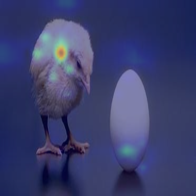
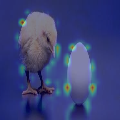
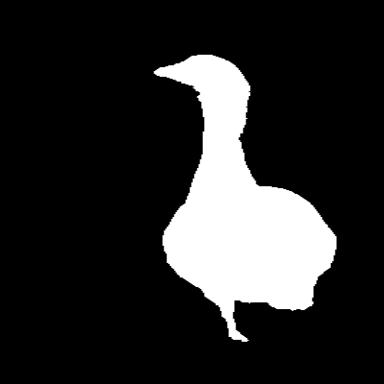
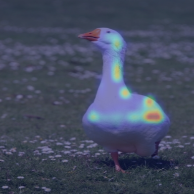
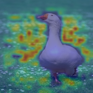
Input	GT	Layer 1	Layer 12

Figure 2: The visual attention map of the red block in the input image on the first and twelfth layers of the transformer. The attention maps show that features from shallow layer can also have global information and features from deep layer can also have local information.

With the merits mentioned above, we propose a method called Global-Local Saliency TRansformer (GLSTR). The core of our method is a pure transformer-based encoder and a mixed decoder to aggregate features generated by transformers. To encode features through transformers, we first split the input image into a grid of fixed-size patches. We use a linear projection layer to map each image patch to a feature vector for representing local details. By passing the feature through the multi-head self-attention module in each transformer layer, the model further encodes global features without diluting the local ones. To decode the features with global-local information over the inputs and the previous layer from the transformer encoder, we propose to densely decode feature from each transformer layer. With this dense connection, the representations during decoding still preserve rich local and global features. To the best of our knowledge, we are the first work to apply the pure transformer-based encoder on SOD tasks.

To sum up, our contributions are in three folds:

• We unify global-local representations with a novel transformer-based architecture, which models long-range dependency within each layer.

• To take full advantage of the global information of previous layers, we propose a new decoder, deeply-transformed decoder, to densely decode features of each layer.

• We conduct extensive evaluations on five widely-used benchmark datasets, showing that our method outperforms state-of-the-art methods by a large margin, with an average of $12.17\%$ improvement in terms of MAE.

2 Related Work

Salient Object Detection. FCN has became the mainstream architecture for the saliency detection methods, to predict pixel-wise saliency maps directly [20, 40, 39, 51, 23, 55, 14, 31, 36]. Especially, the skip-connection architecture has been demonstrated its performance in combining global and local context information [16, 59, 22, 52, 26, 41, 34]. Hou et al. [16] proposed that the high-level features are capable of localizing the salient regions while the shallower ones are active at preserving low-level details. Therefore, they introduced short connections between the deeper and shallower feature pairs. Based on the U-Shape architecture, Zhao et al. [59] introduced a transition layer and a gate into every skip connection, to suppress the misleading convolutional information in the original features from the encoder. In order to localize the salient objects better, they also built a Fold-ASPP module on the top of the encoder. Similarly, Liu et al. [22] inserted a pyramid pooling module on the top of the encoder to capture the high-level semantic information. In order to recover the diluted information in the convolutional encoder and alleviate the coarse-level feature aggregation problem while decoding, they introduced a feature aggregation module after every skip connection. In [57], Zhao et al. adopted the VGG network without fully connected layers as their backbone. They fused the high-level feature into the shallower one at each scale to recover the diluted location information. After three convolution layers, each fused feature was enhanced by the saliency map. Specifically, they introduced the edge map as a guidance for the shallowest feature and fused this feature into deeper ones to produce the side outputs.

Aforementioned methods usually suffer from the limited size of convolutional operation. Although there will be large receptive fields in the deep convolution layers, the low-level information is diluted increasingly with the increasing number of layers.

Transformer. Since the local information covered by the convolutional operation is deficient, numerous methods adopt attention mechanisms to capture the long-range correlation [43, 1, 17, 56, 37]. The transformer, proposed by Vaswani et al. [35], has demonstrated its global-attention performance in machine translation task. Recently, more and more works focus on exploring the ability of transformer in computer vision tasks. Dosovitskiy et al. [9] proposed to apply the pure transformer directly to sequences of image patches for exploring spatial correlation on image classification tasks. Carion et al.  [2] proposed a transformer encoder-decoder architecture on object detection tasks. By collapsing the feature from CNN into a sequence of learned object queries, the transformer can dig out the correlation between objects and the global image context. Zeng et al. [50] proposed a spatial-temporal transformer network to tackle video inpainting problem along spatial and temporal channel jointly.

The most related work to ours is [60]. They proposed to replace the convolution layers with the pure transformer during encoding for semantic segmentation task. Unlike this work, we propose a transformer based U-shape architecture network that is more suitable for dense prediction tasks. With our dense skip-connections and progressive upsampling strategy, the proposed method can sufficiently associate the decoding features with the global-local ones from the transformer.

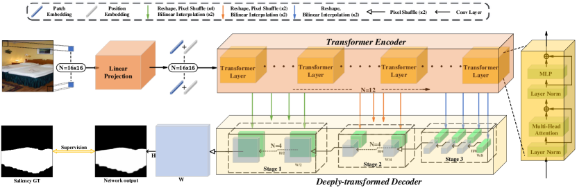
Figure 3: The pipeline of our proposed method. We first divide the image into non-overlap patches and map each patch into the token before feeding to transformer layers. After encoding features through 12 transformer layers, we decode each output feature in three successive stages with 8$\times$, 4$\times$, and 2$\times$ upsampling respectively. Each decoding stage contains four layers and the input of each layer comes from the features of its previous layer together with the corresponding transformer layer.

3 Method

In this paper, we propose a Global-Local Saliency TRansfromer (GLSTR) which models the local and global representations jointly in each encoder layer and decodes all features from transformers with gradual spatial resolution recovery. In the following subsections, we first review the local and global feature extraction by the fully convolutional network-based salient object detection methods in Sec. 3.1. Then we give more details about how the transformer extracts global and local features in each layer in Sec. 3.2. Finally, we specify different decoders including naive decoder, stage-by-stage decoder, multi-level feature aggregation decoder [60], and our proposed decoder. The framework of our proposed method is shown in Fig. 3.

3.1 FCN-based Salient Object Detection

We revisit traditional FCN based salient object detection methods on how to extract global-local representations. Normally, a CNN-based encoder (e.g., VGG [34] and ResNet [13]) takes an image as input. Due to the locality of CNN, a stack of convolution layers is applied to the input images. At the same time, the spatial resolution of the feature maps gradually reduces at the end of each stage. Such an operation extends the receptive field of the encoder and reaches a global view in deep layers. This kind of encoder faces three serious problems: 1) features from deep layers have a global view with diluted local details due to too much convolution operations and resolution reduction; 2) features from shallow layers have more local details but lack of semantic understanding to identify salient objects, due to the locality of the convolution layers; 3) features from adjacent layers have limited variances and lead to redundancy when they are densely decoded.

Recent work focuses on strengthening the ability to extract either local details or global semantics. To learn local details, previous works [57, 42, 46] focus on features from shallow layers by adding edge supervision. Such low-level features lack a global view and may misguide the whole network. To learn global semantics, attention mechanism is used to enlarge the receptive field. However, previous works [4, 55] only apply the attention mechanism in deep layers (e.g. , the last layer of the encoder). In the following subsections, we demonstrate how to preferably unify local-global features using the transformer.

3.2 Transformer Encoder

3.2.1 Image Serialization

Since the transformer is designed for the 1D sequence in natural language processing tasks, we first map the input 2D images into 1D sequences. Specifically, given an image $x\in\mathcal{R}^{H\times W\times c}$ with height $H$, width $W$ and channel $c$, the 1D sequence $x^{\prime}\in\mathcal{R}^{L\times C}$ is encoded from the image $x$. A simple idea is to directly reshape the image into a sequence, namely, $L=H\times W$. However, due to the quadratic spatial complexity of self-attention, such an idea leads to enormous GPU memory consumption and computation cost. Inspired by ViT [9], we divide the image $x$ into $\frac{HW}{256}$ non-overlapping image patches with a resolution of $16\times 16$. Then we project these patches into tokens with a linear layer, and the sequence length $L$ is $\frac{HW}{256}$. Every token in $x^{\prime}$ represents a non-overlay $16\times 16$ patch. Such an operation trades off the spatial information and sequence length.

3.2.2 Transformer

Taking 1D sequence $x^{\prime}$ as the input, we use pure transformer as the encoder instead of CNN used in previous works [44, 30, 29]. Rather than only having limited receptive field as CNN-based encoder, with the power of modeling global representations in each layer, the transformer usually requires much fewer layers to receive a global receptive. Besides, the transformer encoder has connections across each pair of image patches. Based on these two characteristics, more local detailed information is preserved in our transformer encoder. Specifically, the transformer encoder contains positional encoding and transformer layers with multi-head attention and multi-layer perception.

Positional Encoding. Since the attention mechanism cannot distinguish the positional difference, the first step is to feed the positional information into sequence $x^{\prime}$ and get the position enhanced feature $F_{0}$:

$$F_{0}=[x^{{}^{\prime}}_{0},x^{{}^{\prime}}_{1},...,x^{{}^{\prime}}_{L}]+E_{pos},$$ (1)

where $+$ is the addition operation and $E_{pos}$ indicates the positional code which is randomly initialized under truncated Gaussian distribution and is trainable in our method.

Transformer Layer. The transformer encoder contains 17 transformer layers, and each layer contains multi-head self-attention (MSA) and multi-layer perceptron (MLP). The multi-head self-attention is the extension of self-attention (SA):

$$\centering\begin{split}Q=FW_{q},K=FW_{k},V=FW_{v},\\ SA(F)=\phi(\frac{QK^{T}}{\sqrt{d}})V,\end{split}\@add@centering$$ (2)

where $F$ indicates the input features of the self-attention, and $W_{q},W_{k},W_{v}$ are the weights with the trainable parameters. d is the dimension of $Q,K,V$ and $\phi(\star)$ is the softmax function. To apply multiple attentions in parallel, multi-head self-attention has $m$ independent self-attentions:

$$MSA(F)=SA_{1}(F)\oplus SA_{2}(F)\oplus...\oplus SA_{m}(F),$$ (3)

where $\oplus$ indicates the concatenation. To sum up, in the $i_{th}$ transformer layer, the output feature $F_{i}$ is calculated by:

$$\begin{split}&\hat{F}_{i}=MSA(LN(F_{i-1}))+F_{i-1},\\ &F_{i}=MLP(LN(\hat{F}_{i}))+\hat{F}_{i},\end{split}$$ (4)

where $LN(\star)$ indicates layer norm and $F_{i}$ is the $i_{th}$ layer features of the transformer.

3.3 Various Decoders

In this section, we design a global-local decoder to decode the features $F\in R^{\frac{HW}{256}\times C}$ from the transformer encoder and generate the final saliency maps $S^{{}^{\prime}}\in R^{H\times W}$ with the same resolution as the inputs. Before exploring the ability of our global-local decoder, we simply introduce the naive decoder, stage-by-stage decoder, and multi-level feature aggregation decoder used in [60] (see Fig. 4). To begin with, we first reshape the features $F_{i}\in R^{\frac{HW}{256}\times C}$ from the transformer into $F^{{}^{\prime}}_{i}\in R^{\frac{H}{16}\times\frac{W}{16}\times C}$.

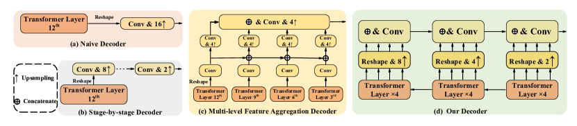
Figure 4: Different types of decoder. Our decoder (d) densely decodes all transformer features and gradually upsamples to the resolution of inputs.

Naive Decoder. As illustrated in Fig. 4(a), a naive idea of decoding transformer features is directly upsampling the outputs of last layer to the same resolution of inputs and generating the saliency maps. Specifically, three conv-batch norm-ReLU layers are applied on $F_{12}$. Then we bilinearly upsample the feature maps 16$\times$, followed by a simple classification layer:

$$\begin{split}Z=Up(CBR(F^{{}^{\prime}}_{12};\theta_{z});16),\\ S^{{}^{\prime}}=\sigma(Conv(Z;\theta_{s})),\end{split}$$ (5)

where $CBR(\star;\theta)$ indicates convolution-batch norm-ReLU layer with parameters $\theta$. $Up(\star;s)$ is the bilinear operation for upsampling $s\times$ and $\sigma$ is the sigmoid function. $S^{\prime}$ is the predicted saliency map.

Stage-by-Stage Decoder. Directly upsampling 16$\times$ at one time like the naive decoder will inject too much noise and lead to coarse spatial details. Inspired by previous FCN-based methods [30] in salient object detection, stage-by-stage decoder which upsamples the resolution 2$\times$ in each stage will mitigate the losses of spatial details seen in Fig. 4(b). Therefore, there are four stages, and in each stage, a decoder block contains three conv-batch norm-ReLU layers:

$$\begin{split}&Z_{0}=CBR(F^{{}^{\prime}}_{12};\theta_{0}),\\ &Z_{i}=CBR(Up(Z_{i-1};2);\theta_{i}),\\ &S^{{}^{\prime}}=\sigma(Conv(Z_{4};\theta_{s})).\end{split}$$ (6)

Multi-level feature Aggregation. As illustrated in Fig. 4(c), Zheng et al.  [60] propose a multi-level feature aggregation to sparsely fuse multi-level features following the similar setting of pyramid network. Rather than having a pyramid shape, the spatial resolutions of features keep the same in the transformer encoder.

Specifically, the decoder take features $F_{3},F_{6},F_{9},F_{12}$ from the $3_{rd},6_{th},9_{th},12_{th}$ layers and upsample them 4$\times$ following several convolutional layers. Then features are top-down aggregated via element-wise addition. Finally, the features from all streams are fused to generate the final saliency maps.

Deeply-transformed Decoder. As illustrated in Fig. 4(d), to combine the benefit from the features of each transformer layer and include less noise injection from upsampling, we gradually integrate all transformer layer features and upsample them into the same spatial resolution of the input images. Specifically, we first divide the transformer features into three stages and we upsample them $8\times,4\times,2\times$ from the first to the third stage respectively. Note that the upsampling operation includes pixel shuffle ($2^{3-n}\times$) and bilinear upsampling (2$\times$), where $n$ indicates the $n_{th}$ stage. In the $j_{th}$ layer of the $i_{th}$ stage, the salient feature $Z_{i,j}$ comes from the concatenation of the transformer feature $F_{i*4+j}$ from the corresponding layer together with the salient feature from the previous layer. A convolution block is applied after upsampling $F^{{}^{\prime}}_{12}$ for $Z_{3,4}$.

$$\small Z_{i,j}=\begin{cases}CBR(Z_{i,j-1}\oplus Up(F^{{}^{\prime}}_{i*4+j};2^{i});\theta_{i,j})~{}~{}~{}~{}~{}~{}~{}~{}j=1,2,3,&\\ CBR(Up(Z_{i-1,j};2)\oplus Up(F^{{}^{\prime}}_{i*4+j};2^{i});\theta_{i,j})~{}~{}~{}~{}j=4.&\end{cases}$$ (7)

Then we simply apply a convolutional operation on salient features $Z_{i,j}$ to generate the final saliency maps $S^{{}^{\prime}}_{i,j}$. Therefore, in our method, we have twelve output saliency maps:

$$S^{{}^{\prime}}_{i,j}=\sigma(Conv(Up(Z_{i,j};2);\theta_{s_{i,j}})).$$ (8)

4 Experiment

Method		DUTS-TE			DUT-OMRON			HKU-IS			ECSSD			PASCAL-S
		MAE $\downarrow$	$F_{\beta}$ $\uparrow$	$\mathcal{S}$ $\uparrow$	MAE $\downarrow$	$F_{\beta}$ $\uparrow$	$\mathcal{S}$ $\uparrow$	MAE $\downarrow$	$F_{\beta}$ $\uparrow$	$\mathcal{S}$ $\uparrow$	MAE $\downarrow$	$F_{\beta}$ $\uparrow$	$\mathcal{S}$ $\uparrow$	MAE $\downarrow$	$F_{\beta}$ $\uparrow$	$\mathcal{S}$ $\uparrow$
DSS	C	0.056	0.801	0.824	0.063	0.737	0.790	0.040	0.889	0.790	0.052	0.906	0.882	0.095	0.809	0.797
UCF	C	0.112	0.742	0.782	0.120	0.698	0.760	0.062	0.874	0.875	0.069	0.890	0.883	0.116	0.791	0.806
Amulet	C	0.085	0.751	0.804	0.098	0.715	0.781	0.051	0.887	0.886	0.059	0.905	0.891	0.100	0.810	0.819
BMPM	C	0.049	0.828	0.862	0.064	0.734	0.809	0.039	0.910	0.907	0.045	0.917	0.911	0.074	0.836	0.846
RAS	C	0.059	0.807	0.838	0.062	0.753	0.814	-	-	-	0.056	0.908	0.893	0.104	0.803	0.796
PSAM	C	0.041	0.854	0.879	0.057	0.765	0.830	0.034	0.918	0.914	0.040	0.931	0.920	0.075	0.847	0.851
CPD	C	0.043	0.841	0.869	0.056	0.754	0.825	0.034	0.911	0.906	0.037	0.927	0.918	0.072	0.837	0.847
SCRN	C	0.040	0.864	0.885	0.056	0.772	0.837	0.034	0.921	0.916	0.038	0.937	0.927	0.064	0.858	0.868
BASNet	C	0.048	0.838	0.866	0.056	0.779	0.836	0.032	0.919	0.909	0.037	0.932	0.916	0.078	0.836	0.837
EGNet	C	0.039	0.866	0.887	0.053	0.777	0.841	0.031	0.923	0.918	0.037	0.936	0.925	0.075	0.846	0.853
MINet	C	0.037	0.865	0.884	0.056	0.769	0.833	0.029	0.926	0.919	0.034	0.938	0.925	0.064	0.852	0.856
LDF	C	0.034	0.877	0.892	0.052	0.782	0.839	0.028	0.929	0.920	0.034	0.938	0.924	0.061	0.859	0.862
GateNet	C	0.040	0.869	0.885	0.055	0.781	0.838	0.033	0.920	0.915	0.040	0.933	0.920	0.069	0.852	0.858
SAC	C	0.034	0.882	0.895	0.052	0.804	0.849	0.026	0.935	0.925	0.031	0.945	0.931	0.063	0.868	0.866
Naive	T	0.043	0.855	0.878	0.059	0.776	0.835	0.042	0.905	0.903	0.042	0.927	0.919	0.068	0.854	0.862
SETR	T	0.039	0.869	0.888	0.056	0.782	0.838	0.037	0.917	0.912	0.041	0.930	0.921	0.062	0.867	0.859
VST	T	0.037	0.877	0.896	0.058	0.800	0.850	0.030	0.937	0.928	0.034	0.944	0.932	0.067	0.850	0.873
Ours	T	0.029	0.901	0.912	0.045	0.819	0.865	0.026	0.941	0.932	0.028	0.953	0.940	0.054	0.882	0.881

Table 1: Quantitative comparisons with FCN-based (denoted as C) and Transformer-based (denoted as T) salient object detection methods by three evaluation metrics. Top three performances are marked in Red, Green, and Blue respectively. Simply utilizing transformer (Naive) achieves comparable performance. Our method significantly outperforms all competitors regardless of what basic component they used (i.e., either FCN or transformer-based).The results of VST${\dagger}$ come from the paper due to the lack of released code or saliency maps.

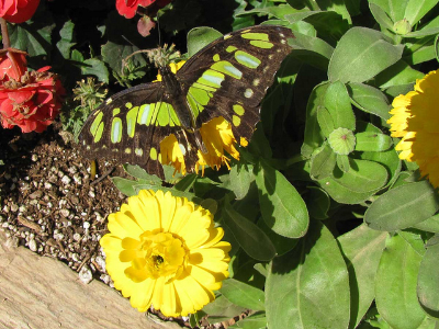
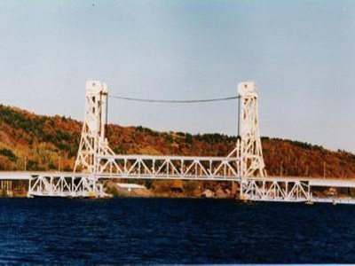
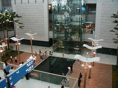
(a) Image

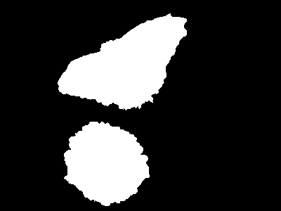
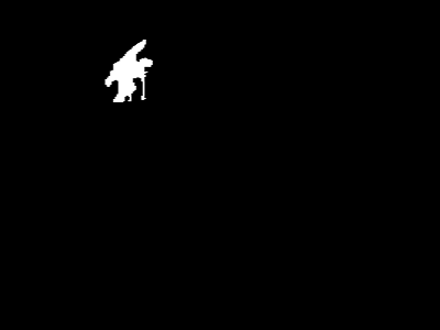
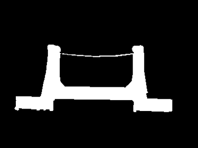
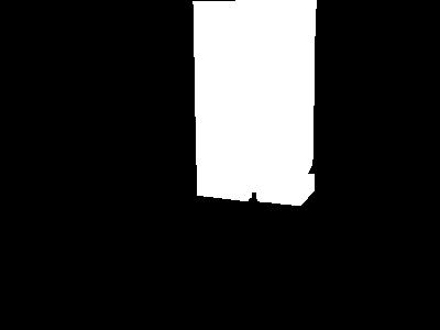
(b) GT

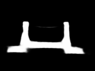
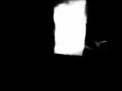
(c) Ours (T)

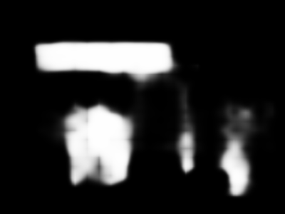
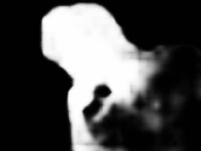
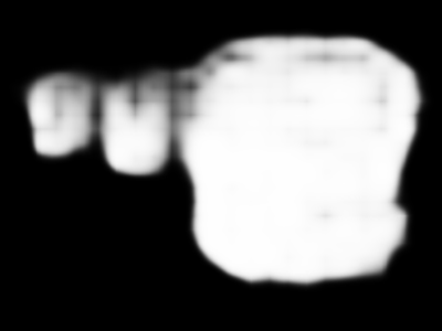
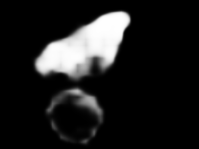
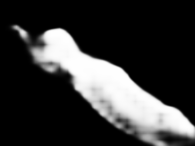
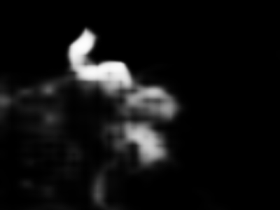
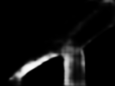
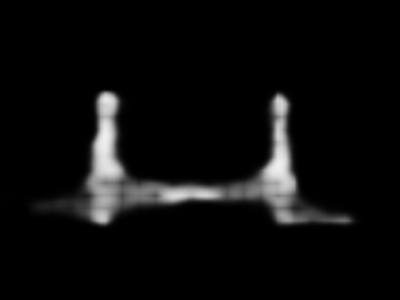
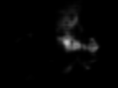
(d) SETR (T)

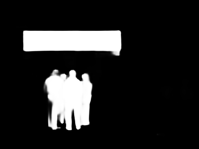
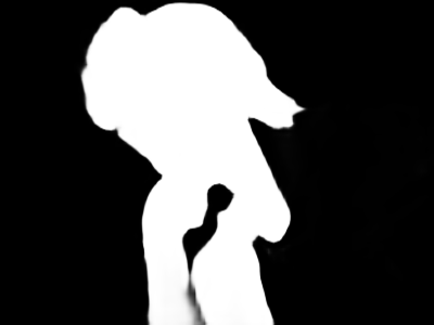
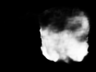
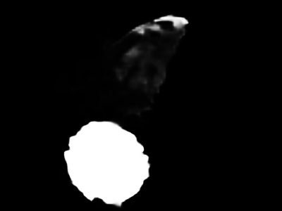
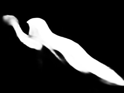
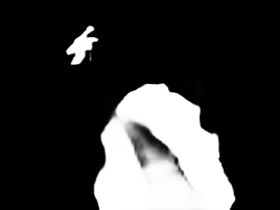
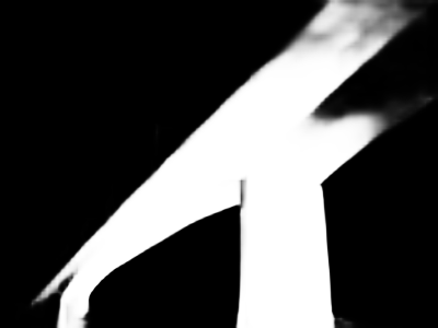
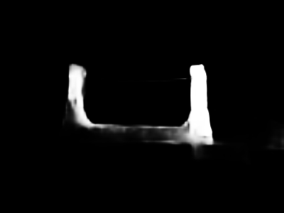
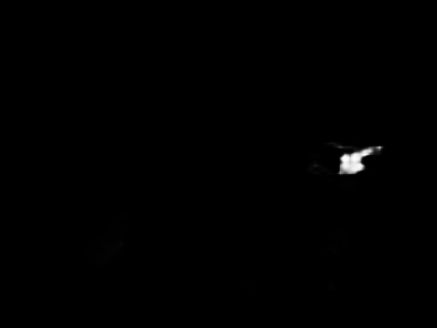
(e) GateNet (C)

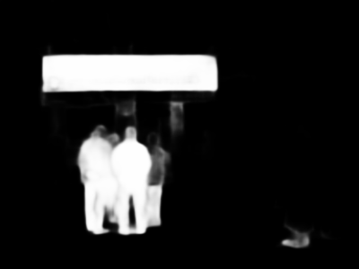
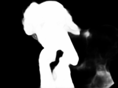
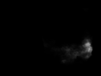
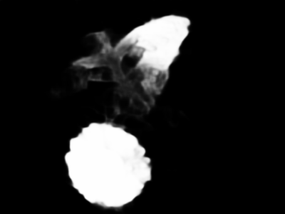
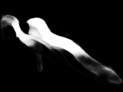
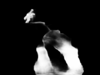
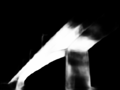
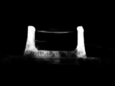
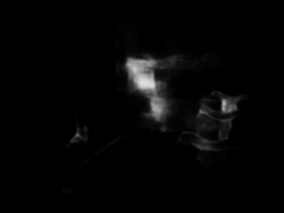
(f) LDF (C)

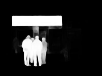
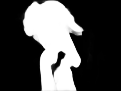
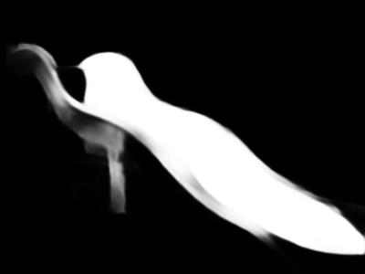
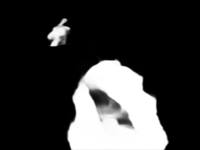
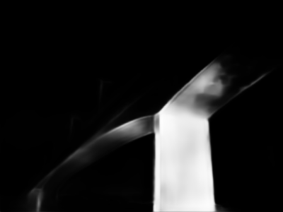
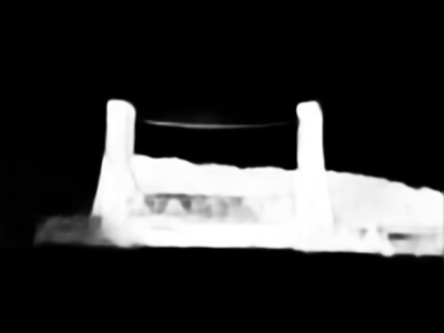
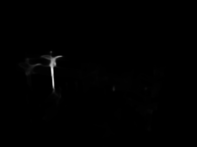
(g) EGNet (C)

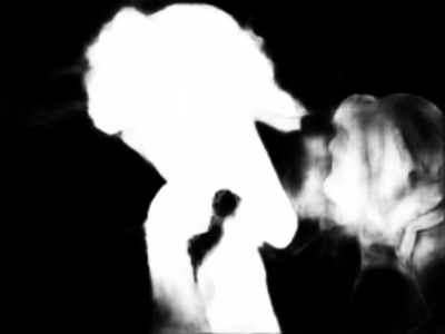
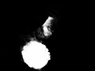
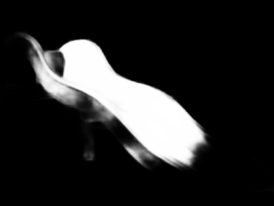
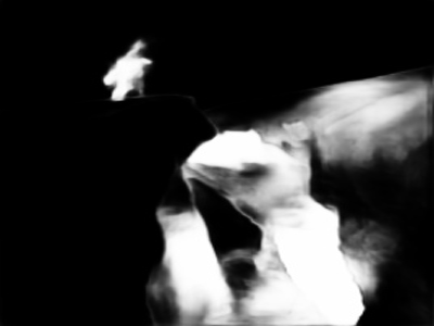
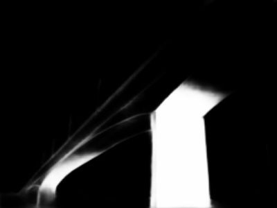
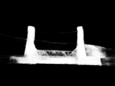
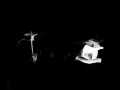
(h) BMPM (C)

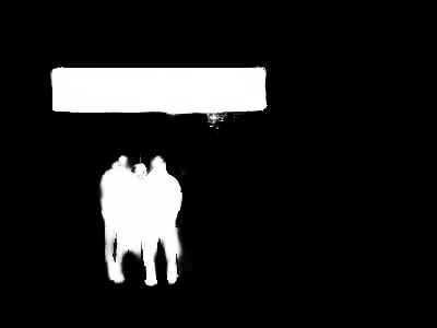
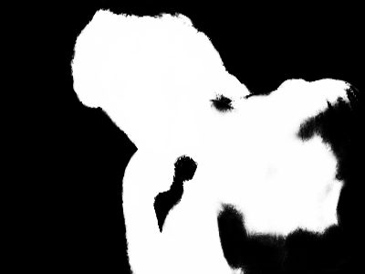
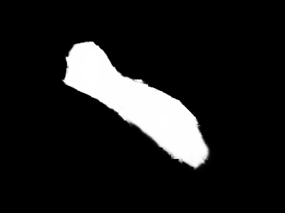
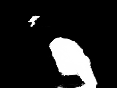
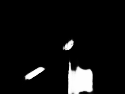
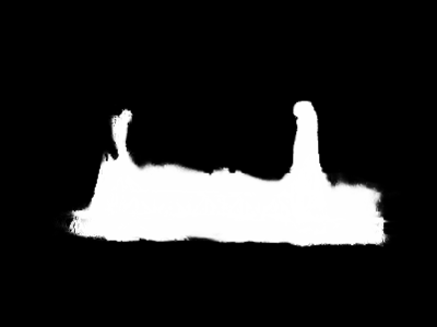
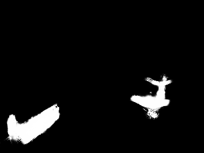
(i) DSS (C)

Figure 5: Qualitative comparisons with state-of-the-art methods. Our method provides more visually reasonable saliency maps by accurately locating salient objects and generating sharp boundaries than other transformer-based (denoted as T) and FCN-based methods (denoted as C).

4.1 Implementation Details

We train our model on DUTS following the same setting as [57]. The transformer encoder is pretrained on ImageNet [9] and the rest layers are randomly initialized following the default settings in PyTorch. We use SGD with momentum as the optimizer. We set momentum = 0.9, and weight decay = 0.0005. The learning rate starts from 0.001 and gradually decays to 1e-5. We train our model for 40 epochs with a batch size of 8. We adopt vertical and horizontal flipping as the data augmentation techniques. The input images are resized to 384$\times$384. During the inference, we take the output of the last layer as the final prediction.

4.2 Datasets and Loss Function

We evaluate our methods on five widely used benchmark datasets: DUT-OMRON [48], HKU-IS [19], ECSSD [33], DUTS [38], PASCAL-S [21]. DUT-OMRON contains 5,169 challenging images which usually have complex background and more than one salient objects. HKU-IS has 4,447 high-quality images with multiple disconnected salient objects in each image. ECSSD has 1,000 meaningful images with various scenes. DUTS is the largest salient object detection dataset including 10,533 training images and 5,019 testing images. PASCAL-S chooses 850 images from PASCAL VOC 2009.

We use standard binary cross entropy loss as our loss function. Given twelve outputs, we design the final loss as:

$$\begin{split}l_{bce}(S^{{}^{\prime}},S)&=S\log S^{{}^{\prime}}+(1-S)\log(1-S^{{}^{\prime}}),\\ L&=\sum\limits_{i=1}^{3}\sum\limits_{j=1}^{4}l_{bce}(S^{{}^{\prime}}_{i,j},S),\end{split}$$ (9)

where $\{S^{{}^{\prime}}_{i}\}$ indicate our predicted saliency maps and $S$ indicates the ground truth.

4.3 Evaluation Metrics

In this paper, we evaluate our methods under three widely used evaluation metrics: mean absolute error (MAE), weighted F-Measure ($F_{\beta}$), and S-Measure ($S$) [12].

MAE directly measures the average pixel-wise differences between saliency maps and labels by mean absolute error:

$$MAE(S^{{}^{\prime}},S)=\left|S^{{}^{\prime}}-S\right|.$$ (10)

$F_{\beta}$ evaluates the precision and recall at the same time and use $\beta^{2}$ to weight precision:

$$F_{\beta}=\frac{(1+\beta^{2})\times Precision\times Recall}{\beta^{2}\times Precision+Recall},$$ (11)

where $\beta^{2}$ is set to 0.3 as in previous work [57].

S-Measure strengthens the structural information of both foreground and background. Specifically, the regional similarity $S_{r}$ and the object similarity $S_{o}$ are combined together with weight $\alpha$:

$$S=\alpha*S_{o}+(1-\alpha)*S_{r},$$ (12)

where $\alpha$ is set to 0.5 [57].

4.4 Comparison with state-of-the-art methods

We compare our method with 12 state-of-the-art salient object detection methods: DSS [16], UCF [54], Amulet [53] BMPM [51],RAS [5], PSAM[3] PoolNet [22], CPD [45], SCRN [47], BASNet [30], EGNet [57], MINet [29], LDF [44], GateNet [59], SAC [18], SETR [60], VST [10], and Naive (Transformer encoder with the naive decoder). The saliency maps are provided by their authors or calculated by the released code except SETR and Naive which are implemented by ourselves. Besides, all results are evaluated with the same evaluation code.

Quantitative Comparison. We report the quantitative results in Tab. 1. As can be seen from these results, with out any post-processing, our method outperforms all compared methods using FCN-based or transformer-based architecture by a large margin on all evaluation metrics. In particular, the performance is averagely improved 12.17% over the second best method LDF in terms of MAE. The superior performance on both easy and difficult datasets shows that our method does well on both simple and complex scenes. Another interesting finding is that transformer is powerful to generate rather good saliency maps with “Naive” decoder, although it cannot outperform state-of-the-art FCN-based method (i.e., SAC). Further investigating the potential for transformer may keep enhancing the performance on salient object detection task.

Qualitative Comparison. The qualitative results are shown in Fig. 5. With the power of modeling long range dependency over the whole image, transformer-based methods are able to capture the salient object more accurately. For example, in the sixth row of Fig. 5, our method can accurately capture the salient object without being deceived by the ice hill while FCN-based methods all fail in this case. Besides, saliency maps predicted by our method are more complete, and aligned with the ground truths.

4.5 Ablation Study

In this subsection, we mainly evaluate the effectiveness of dense connections and different upsampling strategies in our decoder design on two challenging datasets: DUTS-TE and DUT-OMRON.

Effectiveness of Dense Connections.

Input	GT	Dens.4	Dens.3	Dens.2	Dens.1	Dens.0
		Ours				Naive

Figure 6: The effect of dense connection during decoding. We gradually increase the density of connection between transformer output features and decoding convolution layer in all stages. The naive decoder (i.e., density 0) predicts saliency maps with a lot of noises, which is severely influenced by the background. As the density increasing, the saliency maps become more accurate and sharp, especially near the boundaries.

Density	DUTS-TE			DUT-OMRON
	MAE $\downarrow$	$F_{\beta}$  $\uparrow$	S $\uparrow$	MAE $\downarrow$	$F_{\beta}$ $\uparrow$	S $\uparrow$
0	0.043	0.855	0.878	0.059	0.776	0.835
1	0.033	0.889	0.902	0.052	0.802	0.852
2	0.031	0.895	0.907	0.050	0.807	0.857
3	0.030	0.899	0.910	0.047	0.813	0.862
4	0.029	0.901	0.912	0.045	0.819	0.865

Table 2: Quantitative evaluation on dense connection during decoding. As can be seen, adding connections can bring significant performance gain compared to the naive one (i.e., density=0). As the density increasing, the performance gradually improves on all three evaluation metrics. The best performances are marked as red.

We first conduct an experiment to examine the effect of densely decoding the features from each transformer encoding layer. Starting from simply decoding the features of last transformer (i.e., naive decoder), we gradually add the fuse connections in each stage to increase the density until reaching our final decoder, denoted as density 0, 1, 2, 3. For example, the density 3 means that there are three connections (i.e., from $Z_{i,4},Z_{i,3},Z_{i,2}$) added in each stage and only one (i.e., $Z_{i,4}$) for density 1.

The qualitative results are illustrated in Fig. 6, and quantitative results are shown in Tab. 2. When we use the naive decoder without any connection, the results are much worse with lots of noises. The saliency maps are more sharp and accurate with the increase of decoding density, and the performances also gradually increase on three evaluation metrics. As each layer captures a global view of its previous layer, the representation differences are maximized among different transformer features. Thus, each transformer feature can contribute individually to the predicted saliency maps.

Effectiveness of Upsampling Strategy.

Upsample	DUTS-TE			DUT-OMRON
Strategy	MAE $\downarrow$	$F_{\beta}$  $\uparrow$	S $\uparrow$	MAE $\downarrow$	$F_{\beta}$ $\uparrow$	S $\uparrow$
Density set to 0
16$\times$	0.043	0.855	0.878	0.059	0.776	0.835
Four 2$\times$	0.041	0.861	0.883	0.059	0.775	0.836
Density set to 1
16$\times$	0.036	0.875	0.896	0.052	0.794	0.850
4$\times$ and 4$\times$	0.034	0.886	0.900	0.053	0.801	0.850
Ours	0.033	0.889	0.902	0.052	0.802	0.852
Density set to 4
16$\times$	0.034	0.882	0.902	0.051	0.799	0.846
4$\times$ and 4$\times$	0.030	0.900	0.911	0.047	0.814	0.862
Ours	0.029	0.901	0.912	0.045	0.819	0.865

Table 3: Qualitative evaluations on the upsampling strategies under different density settings. Gradually upsampling leads to better performance than the naive one and our upsampling strategy outperforms others under different density settings.

To evaluate the effect of our gradually upsampling strategy used in the decoder, we compare different upsampling strategies on different density settings. 1) The Naive decoder (denoted as 16$\times$) simply upsamples the last transformer features 16$\times$ for prediction. 2) When density is set to 0, we test an upsampling strategy in stage-by-stage decoder (denoted as Four 2$\times$), where the output features of each stage are upsampled 2$\times$ before sending to the next stage and there are four $2\times$ upsampling operations in total. 3) A sampling strategy (denoted as 4$\times$ and 4$\times$) used in SETR [60] upsamples each transformer features 4$\times$, and another 4$\times$ is applied to obtain the final predicted saliency map. 4) Our decoder (Ours) upsamples transformer features 8$\times$, 4$\times$, 2$\times$ for the layers connected to stage 1, stage 2, stage 3 respectively.

The quantitative results are reported in Tab 3 with some interesting findings. Gradually upsampling always performs better than the naive one with a single $16\times$ upsampling operation. With the help of our upsampling strategy, the dense decoding manifests its advanced performance, with less noise injected during decoding. Directly decoding the output feature from last transformer in Stage mode only leads to limited performance, further indicating the importance of our dense connection.

4.6 The Statistics of Timing

Although the computational cost of transformer encoder may be high, thanks to the parallelism of attention architecture, the inference speed is still comparable to recent methods, shown in Tab. 4. Besides, as a pioneer work, we want to highlight the power of transformer on salient object detection (SOD) task and leave time complexity reduction as the future work.

Method	DSS	R3Net	BASNet	SCRN	EGNet	Ours
Speed(FPS)	24	19	28	16	7	15

Table 4: Running time of different methods. We test all methods on a single RTX2080Ti.

5 Conclusion

In this paper, we explore the unified learning of global-local representations in salient object detection with an attention-based model using transformers. With the power of modeling long range dependency in transformer, we overcome the limitations caused by the locality of CNN in previous salient object detection methods. We propose an effective decoder to densely decode transformer features and gradually upsample to predict saliency maps. It fully uses all transformer features due to the high representation differences and less redundancy among different transformer features. We adopt a gradually upsampling strategy to keep less noise injection during decoding to magnify the ability of locating accurate salient region. We conduct experiments on five widely used datasets and three evaluation metrics to demonstrate that our method significantly outperforms state-of-the-art methods by a large margin.

References

- [1] Irwan Bello, Barret Zoph, Ashish Vaswani, Jonathon Shlens, and Quoc V Le. Attention augmented convolutional networks. In ICCV, pages 3286–3295, 2019.
- [2] Nicolas Carion, Francisco Massa, Gabriel Synnaeve, Nicolas Usunier, Alexander Kirillov, and Sergey Zagoruyko. End-to-end object detection with transformers. In ECCV, pages 213–229. Springer, 2020.
- [3] Jia-Ren Chang and Yong-Sheng Chen. Pyramid stereo matching network. In Proceedings of the IEEE Conference on Computer Vision and Pattern Recognition, pages 5410–5418, 2018.
- [4] Shuhan Chen, Xiuli Tan, Ben Wang, and Xuelong Hu. Reverse attention for salient object detection. In ECCV, pages 234–250, 2018.
- [5] Shuhan Chen, Xiuli Tan, Ben Wang, and Xuelong Hu. Reverse attention for salient object detection. In European Conference on Computer Vision, 2018.
- [6] Ming-Ming Cheng, Niloy J Mitra, Xiaolei Huang, Philip HS Torr, and Shi-Min Hu. Global contrast based salient region detection. IEEE TPAMI, 37(3):569–582, 2014.
- [7] Celine Craye, David Filliat, and Jean-François Goudou. Environment exploration for object-based visual saliency learning. In ICRA, pages 2303–2309. IEEE, 2016.
- [8] Robert Desimone and John Duncan. Neural mechanisms of selective visual attention. Annual review of neuroscience, 18(1):193–222, 1995.
- [9] Alexey Dosovitskiy, Lucas Beyer, Alexander Kolesnikov, Dirk Weissenborn, Xiaohua Zhai, Thomas Unterthiner, Mostafa Dehghani, Matthias Minderer, Georg Heigold, Sylvain Gelly, et al. An image is worth 16x16 words: Transformers for image recognition at scale. arXiv preprint arXiv:2010.11929, 2020.
- [10] Yuming Du, Yang Xiao, and Vincent Lepetit. Learning to better segment objects from unseen classes with unlabeled videos. arXiv preprint arXiv:2104.12276, 2021.
- [11] Wolfgang Einhäuser and Peter König. Does luminance-contrast contribute to a saliency map for overt visual attention? European Journal of Neuroscience, 17(5):1089–1097, 2003.
- [12] Deng-Ping Fan, Ming-Ming Cheng, Yun Liu, Tao Li, and Ali Borji. Structure-measure: A new way to evaluate foreground maps. In ICCV, pages 4548–4557, 2017.
- [13] Kaiming He, Xiangyu Zhang, Shaoqing Ren, and Jian Sun. Deep residual learning for image recognition. In CVPR, pages 770–778, 2016.
- [14] Shengfeng He, Jianbo Jiao, Xiaodan Zhang, Guoqiang Han, and Rynson WH Lau. Delving into salient object subitizing and detection. In ICCV, pages 1059–1067, 2017.
- [15] Shengfeng He and Rynson WH Lau. Saliency detection with flash and no-flash image pairs. In ECCV, pages 110–124. Springer, 2014.
- [16] Qibin Hou, Ming-Ming Cheng, Xiaowei Hu, Ali Borji, Zhuowen Tu, and Philip HS Torr. Deeply supervised salient object detection with short connections. In CVPR, pages 3203–3212, 2017.
- [17] Han Hu, Zheng Zhang, Zhenda Xie, and Stephen Lin. Local relation networks for image recognition. In ICCV, pages 3464–3473, 2019.
- [18] Xiaowei Hu, Chi-Wing Fu, Lei Zhu, Tianyu Wang, and Pheng-Ann Heng. Sac-net: Spatial attenuation context for salient object detection. IEEE Transactions on Circuits and Systems for Video Technology, 2020. to appear.
- [19] G. Li and Y. Yu. Visual saliency based on multiscale deep features. In CVPR, pages 5455–5463, June 2015.
- [20] Guanbin Li and Yizhou Yu. Deep contrast learning for salient object detection. In CVPR, pages 478–487, 2016.
- [21] Yin Li, Xiaodi Hou, Christof Koch, James M Rehg, and Alan L Yuille. The secrets of salient object segmentation. In CVPR, pages 280–287, 2014.
- [22] Jiang-Jiang Liu, Qibin Hou, Ming-Ming Cheng, Jiashi Feng, and Jianmin Jiang. A simple pooling-based design for real-time salient object detection. In CVPR, pages 3917–3926, 2019.
- [23] Nian Liu, Junwei Han, and Ming-Hsuan Yang. Picanet: Learning pixel-wise contextual attention for saliency detection. In CVPR, pages 3089–3098, 2018.
- [24] Jonathan Long, Evan Shelhamer, and Trevor Darrell. Fully convolutional networks for semantic segmentation. In CVPR, pages 3431–3440, 2015.
- [25] Wenfeng Luo, Meng Yang, and Weishi Zheng. Weakly-supervised semantic segmentation with saliency and incremental supervision updating. Pattern Recognition, page 107858, 2021.
- [26] Zhiming Luo, Akshaya Mishra, Andrew Achkar, Justin Eichel, Shaozi Li, and Pierre-Marc Jodoin. Non-local deep features for salient object detection. In CVPR, pages 6609–6617, 2017.
- [27] Roey Mechrez, Eli Shechtman, and Lihi Zelnik-Manor. Saliency driven image manipulation. Machine Vision and Applications, 30(2):189–202, 2019.
- [28] Clifford Thomas Morgan. Physiological psychology. 1943.
- [29] Youwei Pang, Xiaoqi Zhao, Lihe Zhang, and Huchuan Lu. Multi-scale interactive network for salient object detection. In CVPR, June 2020.
- [30] Xuebin Qin, Zichen Zhang, Chenyang Huang, Chao Gao, Masood Dehghan, and Martin Jagersand. Basnet: Boundary-aware salient object detection. In CVPR, June 2019.
- [31] Sucheng Ren, Chu Han, Xin Yang, Guoqiang Han, and Shengfeng He. Tenet: Triple excitation network for video salient object detection. In ECCV, pages 212–228. Springer, 2020.
- [32] John H Reynolds and Robert Desimone. Interacting roles of attention and visual salience in v4. Neuron, 37(5):853–863, 2003.
- [33] Jianping Shi, Qiong Yan, Li Xu, and Jiaya Jia. Hierarchical image saliency detection on extended cssd. IEEE TPAMI, 38(4):717–729, 2015.
- [34] Karen Simonyan and Andrew Zisserman. Very deep convolutional networks for large-scale image recognition. arXiv preprint arXiv:1409.1556, 2014.
- [35] Ashish Vaswani, Noam Shazeer, Niki Parmar, Jakob Uszkoreit, Llion Jones, Aidan N Gomez, Lukasz Kaiser, and Illia Polosukhin. Attention is all you need. arXiv preprint arXiv:1706.03762, 2017.
- [36] Bo Wang, Wenxi Liu, Guoqiang Han, and Shengfeng He. Learning long-term structural dependencies for video salient object detection. IEEE TIP, 29:9017–9031, 2020.
- [37] Huiyu Wang, Yukun Zhu, Bradley Green, Hartwig Adam, Alan Yuille, and Liang-Chieh Chen. Axial-deeplab: Stand-alone axial-attention for panoptic segmentation. In ECCV, pages 108–126. Springer, 2020.
- [38] Lijun Wang, Huchuan Lu, Yifan Wang, Mengyang Feng, Dong Wang, Baocai Yin, and Xiang Ruan. Learning to detect salient objects with image-level supervision. In CVPR, pages 136–145, 2017.
- [39] Linzhao Wang, Lijun Wang, Huchuan Lu, Pingping Zhang, and Xiang Ruan. Saliency detection with recurrent fully convolutional networks. In ECCV, pages 825–841. Springer, 2016.
- [40] Tiantian Wang, Ali Borji, Lihe Zhang, Pingping Zhang, and Huchuan Lu. A stagewise refinement model for detecting salient objects in images. In ICCV, pages 4019–4028, 2017.
- [41] Tiantian Wang, Lihe Zhang, Shuo Wang, Huchuan Lu, Gang Yang, Xiang Ruan, and Ali Borji. Detect globally, refine locally: A novel approach to saliency detection. In CVPR, pages 3127–3135, 2018.
- [42] Wenguan Wang, Shuyang Zhao, Jianbing Shen, Steven CH Hoi, and Ali Borji. Salient object detection with pyramid attention and salient edges. In CVPR, pages 1448–1457, 2019.
- [43] Xiaolong Wang, Ross Girshick, Abhinav Gupta, and Kaiming He. Non-local neural networks. In CVPR, pages 7794–7803, 2018.
- [44] Jun Wei, Shuhui Wang, Zhe Wu, Chi Su, Qingming Huang, and Qi Tian. Label decoupling framework for salient object detection. In CVPR, June 2020.
- [45] Zhe Wu, Li Su, and Qingming Huang. Cascaded partial decoder for fast and accurate salient object detection. In CVPR, June 2019.
- [46] Zhe Wu, Li Su, and Qingming Huang. Stacked cross refinement network for edge-aware salient object detection. In ICCV, pages 7264–7273, 2019.
- [47] Z. Wu, L. Su, and Q. Huang. Stacked cross refinement network for edge-aware salient object detection. In ICCV, pages 7263–7272, 2019.
- [48] Chuan Yang, Lihe Zhang, Huchuan Lu, Xiang Ruan, and Ming-Hsuan Yang. Saliency detection via graph-based manifold ranking. In CVPR, pages 3166–3173, 2013.
- [49] Yang Yang, Jimei Yang, Junjie Yan, Shengcai Liao, Dong Yi, and Stan Z Li. Salient color names for person re-identification. In ECCV, pages 536–551. Springer, 2014.
- [50] Yanhong Zeng, Jianlong Fu, and Hongyang Chao. Learning joint spatial-temporal transformations for video inpainting. In ECCV, pages 528–543. Springer, 2020.
- [51] Lu Zhang, Ju Dai, Huchuan Lu, You He, and Gang Wang. A bi-directional message passing model for salient object detection. In CVPR, pages 1741–1750, 2018.
- [52] Pingping Zhang, Dong Wang, Huchuan Lu, Hongyu Wang, and Xiang Ruan. Amulet: Aggregating multi-level convolutional features for salient object detection. In ICCV, pages 202–211, 2017.
- [53] Pingping Zhang, Dong Wang, Huchuan Lu, Hongyu Wang, and Xiang Ruan. Amulet: Aggregating multi-level convolutional features for salient object detection. In ICCV, Oct 2017.
- [54] Pingping Zhang, Dong Wang, Huchuan Lu, Hongyu Wang, and Baocai Yin. Learning uncertain convolutional features for accurate saliency detection. In ICCV, Oct 2017.
- [55] Xiaoning Zhang, Tiantian Wang, Jinqing Qi, Huchuan Lu, and Gang Wang. Progressive attention guided recurrent network for salient object detection. In CVPR, pages 714–722, 2018.
- [56] Hengshuang Zhao, Jiaya Jia, and Vladlen Koltun. Exploring self-attention for image recognition. In CVPR, pages 10076–10085, 2020.
- [57] Jia-Xing Zhao, Jiang-Jiang Liu, Deng-Ping Fan, Yang Cao, Jufeng Yang, and Ming-Ming Cheng. Egnet: Edge guidance network for salient object detection. In ICCV, pages 8779–8788, 2019.
- [58] Rui Zhao, Wanli Oyang, and Xiaogang Wang. Person re-identification by saliency learning. IEEE TPAMI, 39(2):356–370, 2016.
- [59] Xiaoqi Zhao, Youwei Pang, Lihe Zhang, Huchuan Lu, and Lei Zhang. Suppress and balance: A simple gated network for salient object detection. In ECCV, pages 35–51, 2020.
- [60] Sixiao Zheng, Jiachen Lu, Hengshuang Zhao, Xiatian Zhu, Zekun Luo, Yabiao Wang, Yanwei Fu, Jianfeng Feng, Tao Xiang, Philip HS Torr, et al. Rethinking semantic segmentation from a sequence-to-sequence perspective with transformers. arXiv preprint arXiv:2012.15840, 2020.