Xubo Yue, Maher Nouiehed, Raed Al Kontar

GIFAIR-FL: A Framework for Group and Individual Fairness in Federated Learning

Xubo Yue Industrial & Operations Engineering, University of Michigan, Ann Arbor, MI 48109, USA, maxyxb@umich.edu Maher Nouiehed Industrial Engineering and Management, American University of Beirut, Beirut, Lebanon, mn102@aub.edu.lb Raed Al Kontar Industrial & Operations Engineering, University of Michigan, Ann Arbor, MI 48109, USA, alkontar@umich.edu

In this paper we propose GIFAIR-FL: a framework that imposes Group and Individual FAIRness to Federated Learning settings. By adding a regularization term, our algorithm penalizes the spread in the loss of client groups to drive the optimizer to fair solutions. Our framework GIFAIR-FL can accommodate both global and personalized settings. Theoretically, we show convergence in non-convex and strongly convex settings. Our convergence guarantees hold for both $i.i.d.$ and non-$i.i.d.$ data. To demonstrate the empirical performance of our algorithm, we apply our method to image classification and text prediction tasks. Compared to existing algorithms, our method shows improved fairness results while retaining superior or similar prediction accuracy.

Federated Data Analytics, Fairness, Global Model, Personalized Model, Convergence

1 Introduction

A critical change is happening in today’s Internet of Things (IoT). The computational power of edge devices is steadily increasing. AI chips are rapidly infiltrating the market, smart phones nowadays have compute power comparable to everyday use laptops (Samsung 2019), Tesla just boasted that its autopilot system has computing power of more than 3000 MacBook pros (CleanTechnica 2021) and small local computers such as Raspberry Pis have become common place in many applications especially manufacturing (Al-Ali et al. 2018). This opens a new paradigm for data analytics in IoT; one that exploits local computing power to process more of the user’s data where it is created. This future of IoT has been recently termed as the “The Internet of Federated Things (IoFT)” (Kontar et al. 2021) where the term federated, refers to some autonomy for IoT devices and is inspired by the explosive recent interest in federated data science.

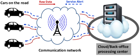
Figure 1: Example of the traditional IoT-enabled System

To give a microcosm of current IoT and its future, consider the IoT teleservice system shown in Fig. 1. Vehicles enrolled in this tele-service system often have their data in the form of condition monitoring signals uploaded to the cloud at regular intervals. The cloud acts as a data processing center that analyzes data for continuous improvement and to keep drivers informed about the health of their vehicles. IoT companies and services, such as Ford’s SYNC and General Motors Onstar services, have long adopted this centralized approach to IoT. However, this state where data is amassed on the cloud yields significant challenges. The need to upload large amounts of data to the cloud incurs high communication and storage costs, demands large internet bandwidth (Jiang et al. 2020, Yang et al. 2020), and leads to latency in deployment as well as reliability risks due to unreliable connection (Zhang et al. 2020c). Further, such a system does not foster trust or privacy as users need to share their raw data which is often sensitive or confidential (Li et al. 2020a).

With the increasing computational power of edge devices, the discussed challenges can be circumvented by moving part of the model learning to the edge. More specifically, rather than processing the data at the cloud, each device performs small local computations and only shares the minimum information needed to allow devices to borrow strength from each other and collaboratively extract knowledge to build smart analytics. In turn, such an approach (i) improves privacy as raw data is never shared, (ii) reduces cost and storage needs as less information is transmitted, (iii) enables learning parallelization and (iv) reduces latency in decisions as many decisions can now be achieved locally. Hereon we will use edge device and client interchangeably, also, the cloud or data processing center is referred to as the central server.

This idea of exploiting the computational power of edge devices by locally training models without recourse to data sharing gave rise to federated learning (FL). In particular, FL is a data analytics approach that allows distributed model learning without access to private data. Although the main concept of FL dates back a while ago, it was brought to the forefront of data science in 2017 by a team at Google which proposed Federated Averaging (FedAvg) (McMahan et al. 2017). In FedAvg, a central server distributes the model architecture (e.g., neural network, linear model) and a global model parameter (e.g., model weights) to selected devices. Devices run local computations to update model parameters and send updated parameters to the server. The server then takes a weighted average of the resulting local parameters to update the global model. This whole process is termed as one communication round and the process is iterated over multiple rounds until an exit condition is met. Figure 2 provides one illustrative example of FedAvg. Since then FL has seen immense success in various fields such as text prediction (Hard et al. 2018, Ramaswamy et al. 2019), Bayesian optimization (Dai et al. 2020, Khodak et al. 2021), Multi-fidelity modeling (Yue and Kontar 2021), environment monitoring (Hu et al. 2018) and healthcare (Li et al. 2020a).

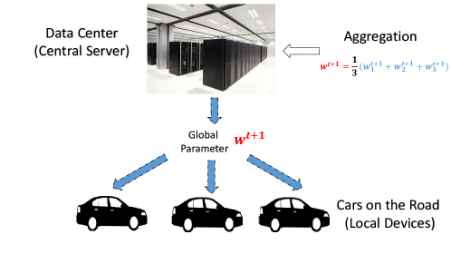
Figure 2: Illustrative Example of FL with FedAvg

Over the last few years, literature has been proposed to improve the performance of FL algorithms; be it speeding up FL algorithms to enable faster convergence (Karimireddy et al. 2020, Yuan and Ma 2020), tackling heterogeneous data both in size and distribution (Zhao et al. 2018, Li et al. 2018, Sattler et al. 2019, Ghosh et al. 2019, Li and Wang 2019), improving the parameter aggregation strategies at the central server (Wang et al. 2020b), designing personalized FL algorithms (Fallah et al. 2020), protecting federated systems from adversarial attacks (Bhagoji et al. 2019, Wang et al. 2020a), and promoting fairness (Li et al. 2019a). Please refer to Kontar et al. (2021) for a detailed literature review. Among those advances, fairness is a critical yet under-investigated area.

In the training phase of FL algorithms, devices with few data, limited bandwidth/memory, or unreliable connection may not be favored by conventional FL algorithms. For instance, as shown in Figure 2, FedAvg samples devices using the weight coefficient $p_{k}$ proportional to the sample size on the device $k$. Scant data on device $k$ will render $p_{k}$ insignificant and this device less favorable by the resulting global model. As a result, such device(s) can potentially incur higher error rate(s). This vicious cycle often relinquishes the opportunity of these devices to significantly contribute in the training process. Indeed, many recent papers have shown the large variety in model performance across devices under FL (Jiang et al. 2019, Hard et al. 2018, Wang et al. 2019, Smith et al. 2017, Kairouz et al. 2019), with some clients showing extremely bad model performance. Besides this aforementioned notion of individual fairness, group fairness also deserves attention in FL. As FL penetrates practical applications, it is important to achieve fair performance across groups of clients characterized by their gender, ethnicity, socio-economic status, geographic location, etc. Despite the importance of this notion of group fairness, unfortunately, no work exists along this line in FL.

Contribution:

We propose a framework, GIFAIR-FL, that aims for fairness in FL. GIFAIR-FL resorts to regularization techniques by penalizing the spread in the loss of clients/groups to drive the optimizer to fair solutions. We show that our regularized formulation can be viewed as a dynamic client re-weighting technique that adaptively gives higher weights to low-performing individuals or groups. Our proposed method adapts the client weights at every communication round accordingly. One key feature of GIFAIR-FL is that it can handle both group-level and individual-level fairness. Also, GIFAIR-FL can be naturally tailored to either a global FL algorithm or a personalized FL algorithm. We then prove that, under reasonable conditions, our algorithm converges to an optimal solution for strongly convex objective functions and to a stationary solution for non-convex functions under non-$\bm{i.i.d}$. settings. Through empirical results on image classification and text prediction datasets, we demonstrate that GIFAIR-FL can promote fairness while achieving superior or similar prediction accuracy relative to recent state-of-the-art fair FL algorithms. Besides that, GIFAIR-FL can be easily plugged into other FL algorithms for different purposes.

Organization:

The rest of the paper is organized as follows. In Sec. 2, we introduce important notations/definitions and briefly review FL. Related work is highlighted in Sec. 2.1. In Sec. 3, we present GIFAIR-FL-Global which is a global modeling approach for fairness in FL. We then briefly discuss the limitation of GIFAIR-FL-Global and introduce GIFAIR-FL-Per which is a personalized alternative for fairness, in Sec. 4. Meanwhile, we provide convergence guarantees for both methods. Experiments on image classification and text prediction tasks are then presented in Sec. 5. Finally, Sec. 6 concludes the paper with a brief discussion.

2 Background

We start by introducing needed background and notation for model development. Then we provide a brief overview of current literature.

Notation: Suppose there are $K\geq 2$ local devices and each device has $N_{k}$ datapoints. Denote by $D_{k}=\big{(}(x_{k,1},y_{k,1}),(x_{k,2},y_{k,2}),\ldots,(x_{k,N_{k}},y_{k,N_{k}})\big{)}$ the data stored at device $k$ where $x\in\mathcal{X}$ is the input, $\mathcal{X}$ is the input space, $y\in\mathcal{Y}$ is the output/label and $\mathcal{Y}$ is the output space. Denote by $\Delta_{\mathcal{Y}}$ the simplex over $\mathcal{Y}$, $h:\mathcal{X}\mapsto\Delta_{\mathcal{Y}}$ the hypothesis and $\mathcal{H}$ a family of hypotheses $h$. Let $\ell$ be a loss function defined over $\Delta_{\mathcal{Y}}\times\mathcal{Y}$. Without loss of generality, assume $\ell\geq 0$. The loss of $h$ is therefore given by $\ell(h(x),y)$. Let $\bm{\theta}\in\bm{\Theta}$ be a vector of parameters defining a hypothesis $h$ and $\bm{\Theta}$ is a parameter space. For instance, $\bm{\theta}$ can be the model parameters of a deep neural network. In the following section we use $h_{\bm{\theta}}$ to represent the hypothesis.

Brief background on FL with FedAvg: In FL, clients collaborate to learn a model that yields better performance relative to each client learning in isolation. This model is called the global model where the global objective function is to minimize the average loss over all clients:

$$\min_{\bm{\theta}}F(\bm{\theta})\coloneqq\sum_{k=1}^{K}p_{k}F_{k}(\bm{\theta}),$$

where $p_{k}=\frac{N_{k}}{\sum_{k}N_{k}}$, $F_{k}(\bm{\theta})=\mathbb{E}_{(x_{k,i},y_{k,i})\sim\mathcal{D}_{k}}[\ell(h_{\bm{\theta}}(x_{k,i}),y_{k,i})]\approx\frac{1}{N_{k}}\sum_{j=1}^{N_{k}}[\ell(h_{\bm{\theta}}(x_{k,j}),y_{k,j})]$ and $\mathcal{D}_{k}$ indicates the data distribution of the $k$-th device’s data observations $(x_{k,i},y_{k,i})$. During training, all devices collaboratively learn global model parameters $\bm{\theta}$ to minimize $F(\bm{\theta})$. The most commonly used method to learn the global objective is FedAvg (McMahan et al. 2017). Details of FedAvg are highlighted in Algorithm 1 as our work will build upon it for fairness. As shown in Algorithm 1, FedAvg aims to learn a global parameter $\bm{\theta}$, by iteratively averaging local updates $\bm{\theta}_{k}$ learned by performing $E$ steps of stochastic gradient descent (SGD) on each client’s local objective $F_{k}$.

Data: number of communication rounds $C$, number of local updates $E$, SGD learning rate schedule $\{\eta^{(t)}\}_{t}$, initial model parameter $\bm{\theta}$

for $c=0:(C-1)$ do

       Select some clients by sampling probability $p_{k}$ and denote by $\mathcal{S}_{c}$ the set of selected clients;

       Server broadcasts $\bm{\theta}$;

       for all selected devices do

             $\bm{\theta}_{k}^{(cE)}=\bm{\theta}$;

             for $t=cE:((c+1)E-1)$ do

                   Randomly sample a subset of data and denote it as $\zeta^{(t)}_{k}$;

                   Local Training $\bm{\theta}^{(t+1)}_{k}=\bm{\theta}^{(t)}_{k}-\eta^{(t)}g_{k}(\bm{\theta}^{(t)}_{k};\zeta^{(t)}_{k})$ ;

                  

             end for

            

       end for

      Aggregation $\bm{\bar{\theta}}_{c}=\frac{1}{|\mathcal{S}_{c}|}\sum_{k\in\mathcal{S}_{c}}\bm{\theta}^{((c+1)E)}_{k}$, Set $\bm{\theta}=\bm{\bar{\theta}}_{c}$;

      

end for

Return $\bm{\bar{\theta}}_{C}$.

Algorithm 1 FedAvg Algorithm (McMahan et al. 2017)

In Algorithm 1, $\zeta_{k}$ denotes the set of indices corresponding to a subset of training data on device $k$ and $g_{k}(\cdot;\zeta_{k})$ denotes the stochastic gradient of $F_{k}(\cdot)$ evaluated on the subset of data indexed by $\zeta_{k}$. Also, $|\mathcal{S}_{c}|$ denotes the cardinality of $\mathcal{S}_{c}$. One should note that it is also common for the central server to sample clients uniformly and then take a weighted average using $p_{k}$ (Li et al. 2019b). Whichever method used, the resulting model may not be fair as small a $p_{k}$ implies a lower weight for client $k$.

Defining fairness in FL: Suppose there are $d\in[2,K]$ groups and each client can be assigned to one of those groups $s\in[d]\coloneqq\{1,\ldots,d\}$. Note that clients from different groups are typically non-$\bm{i.i.d.}$ Denote by $k^{i},k\in[K],i\in[d]$ the index of $k$-th local device in group $i$. Throughout this paper, we drop the superscript $i$ unless we want to emphasize $i$ explicitly. Group fairness can be defined as follows.

Definition 2.1

Denote by $\{a^{i}_{1}\}_{1\leq i\leq d}$ and $\{a^{i}_{2}\}_{1\leq i\leq d}$ the sets of performance measures (e.g., testing accuracy) of trained models 1 and 2 respectively. We say model 1 is more fair than model 2 if $Var(\{a^{i}_{1}\}_{1\leq i\leq d})<Var(\{a^{i}_{2}\}_{1\leq i\leq d})$, where $Var$ is variance.

Definition 2.1 is straightforward: a model is fair if it yields small discrepancies among testing accuracies of different groups. It can be seen that when $d=K$, Definition 2.1 is equivalent to individual fairness (Li et al. 2019a). Definition 1 is widely adopted in FL literature (Mohri et al. 2019, Li et al. 2019a, 2020b, 2021). This notion of fairness might be different from traditional definitions such as demographic disparity (Feldman et al. 2015), equal opportunity and equalized odds (Hardt et al. 2016) in centralized systems. The reason is that those definitions cannot be extended to FL as there is no clear notion of an outcome which is “good” for a device (Kairouz et al. 2019). Instead, fairness in FL can be reframed as equal access to effective models (e.g., the accuracy parity (Zafar et al. 2017) or the representation disparity (Li et al. 2019a)). Specifically, the goal is to train models that incur a uniformly good performance across all devices (Kairouz et al. 2019).

2.1 Literature Overview

Now we briefly review existing state-of-the-art fair and personalized FL algorithms.

Fair FL: Mohri et al. (2019) propose a minimax optimization framework named agnostic FL (AFL). AFL optimizes the worst weighted combination of local devices and is demonstrated to be robust to unseen testing data. Du et al. (2020) further refine the notation of AFL and propose the AgnosticFair algorithm. Specifically, they linearly parametrize weight parameters by kernel functions and show that AFL can be viewed as a special case of AgnosticFair. Upon that, Hu et al. (2020) combine minimax optimization with gradient normalization techniques to produce a fair algorithm FedMGDA+. Motivated by fair resource allocation problems, Li et al. (2019a) propose $q$-Fair FL (q-FFL). q-FFL reweights loss functions such that devices with poor performance will be given relatively higher weights. The q-FFL objective is proved to encourage individual fairness in FL. However, this algorithm requires accurate estimation of a local Lipschitz constant $L$. Later, Li et al. (2020b) developed a tilted empirical risk minimization (TERM) algorithm to handle outliers and class imbalance in statistical estimation procedures. TERM has been shown to be superior to q-FFL in many FL applications. Along this line, Huang et al. (2020) propose to use training accuracy and frequency to adjust weights of devices to promote fairness. Zhang et al. (2020a) develop an algorithm to minimize the discrimination index of the global model to encourage fairness. Here we note that recent work study collaborative fairness in FL (Zhang et al. 2020b, Xu and Lyu 2020, Lyu et al. 2020). The goal of this literature, which is perpendicular to our purpose, is to provide more rewards to high-contributing participants while penalizing free riders.

Personalized FL: One alternative to global modeling is personalized FL which allows each client to retain their own individualized parameters $\{\bm{\theta}_{k}\}_{k=1}^{K}$. For instance, in Algorithm 1 and after training is done, each device $i$ can use $\bm{\theta}=\bm{\bar{\theta}}_{C}$ as the initial weight and run additional SGD steps to obtain a personalized solution $\bm{\theta}_{i}$. Though personalization techniques do not directly target fairness, recent papers have shown that personalized FL algorithms may improve fairness. Arivazhagan et al. (2019) and Liang et al. (2020) use different layers of a network to represent global and personalized solutions. Specifically, they fit personalized layers to each local device such that each device will return a task-dependent solution based on its own local data. Wang et al. (2019), Yu et al. (2020), Dinh et al. (2020) and Li et al. (2021) resort to fine-tuning techniques to learn personalized models. Notably, Li et al. (2021) develops a multi-task personalized FL algorithm Ditto. After optimizing a global objective function, Ditto allows local devices to run more steps of SGD, subject to some constraints, to minimize their own losses. Li et al. (2021) have shown that Ditto can significantly improve testing accuracy among local devices and encourage fairness.

Features of GIFAIR-FL: We here give a quick comparison to highlight the features of our proposed algorithm. The detailed formulation of GIFAIR-FL will be presented in the following section. GIFAIR-FL resorts to regularization to penalize the spread in the loss of client groups. Interestingly, GIFAIR-FL can be seen as a dynamic re-weighting strategy based on the statistical ordering of client/group losses at each communication round. As such, our approach aligns with FL literature that uses re-weighting client schemes, yet existing work faces some limitations. Specifically, AFL and its variants (Mohri et al. 2019, Li et al. 2019a, Hu et al. 2020, Du et al. 2020) exploit minimax formulations that optimize the worst-case distribution of weights among clients to promote fairness. Such approaches lead to overly pessimistic solutions as they only focus on the device with the largest loss. As will be shown in our case studies, GIFAIR-FL significantly outperforms such approaches. Adding to this key advantage, GIFAIR-FL enjoys convergence guarantees even for non-$i.i.d.$ data and is amenable to both global and personalized modeling.

3 GIFAIR-FL-Global: a Global Model for Fairness

We start by detailing our proposed global modeling approach - GIFAIR-FL-Global. In this approach, all local devices collaborate to learn one global model parameter $\bm{\theta}$. Our fair FL formulation aims at imposing group fairness while minimizing the training error. More specifically, our goal is to minimize the discrepancies in the average group losses while achieving a low training error. By penalizing the spread in the loss among client groups, we propose a regularization framework for computing optimal parameters $\bm{\theta}$ that balances learning accuracy and fairness. This translates to solving the following optimization problem

$$\min_{\bm{\theta}}\;H(\bm{\theta})\triangleq\sum_{k=1}^{K}p_{k}F_{k}(\bm{\theta})+\lambda\sum_{1\leq i<j\leq d}|L_{i}(\bm{\theta})-L_{j}(\bm{\theta})|,$$ (1)

where $\lambda$ is a positive scalar that balances fairness and goodness-of-fit, and

$$L_{i}(\bm{\theta})\triangleq\dfrac{1}{|{\cal A}_{i}|}\sum_{k\in{\cal A}_{i}}F_{k}(\bm{\theta})$$

is the average loss for client group $i$, ${\cal A}_{i}$ is the set of indices of devices that belong to group $i$, and $|\mathcal{A}|$ is the cardinality of the set $\mathcal{A}$.

Remark 3.1

Objective (1) aims at ensuring fairness by reducing client loss spread when losses are evaluated at a single global parameter $\bm{\theta}$. This achieves fairness from the server perspective. Specifically, the goal is to find a single solution that yields small discrepancies among $\{L_{i}(\bm{\theta})\}_{i=1}^{d}$.

In typical FL settings, the global objective is given as

$$H(\bm{\theta})=\sum_{k=1}^{K}\,p_{k}H_{k}(\bm{\theta})$$

where each client uses local data to optimize a surrogate of the global objective function. For instance, FedAvg simply uses the local objective function $H_{k}(\bm{\theta})=F_{k}(\bm{\theta})$ for a given client $k$. Interestingly, our global objective in (1) can also be written as $H(\bm{\theta})=\sum_{k=1}^{K}\,p_{k}H_{k}(\bm{\theta})$ as shown in Lemma 3.2 below.

Lemma 3.2

Let $s_{k}\in[d]$ denote the group index of device $k$. For any given $\bm{\theta}$, the global objective function $H(\bm{\theta})$ defined in (1) can be expressed as

$$H(\bm{\theta})=\sum_{k=1}^{K}p_{k}\,\left(1+\dfrac{\lambda}{p_{k}|{\cal A}_{s_{k}}|}r_{k}(\bm{\theta})\right)F_{k}(\bm{\theta}),$$ (2)

where

$$r_{k}(\bm{\theta})=\sum_{1\leq j\neq s_{k}\leq d}{\mbox{sign}}(L_{s_{k}}(\bm{\theta})-L_{j}(\bm{\theta})).$$

Consequently,

$$H(\bm{\theta})=\sum_{k=1}^{K}\,p_{k}H_{k}(\bm{\theta})$$

such that the local client objective is,

$$H_{k}(\bm{\theta})\triangleq\left(1+\dfrac{\lambda}{p_{k}\,|{\cal A}_{s_{k}}|}r_{k}(\bm{\theta})\right)F_{k}(\bm{\theta}).$$ (3)

In Lemma 3.2, $r_{k}(\bm{\theta})\in\{-d+1,-d+3,\ldots,d-3,d-1\}$ is a scalar directly related to the statistical ordering of $L_{s_{k}}$ among client group losses. To illustrate that in a simple example, suppose that at a given $\bm{\theta}$, we have $L_{1}(\bm{\theta})\geq L_{2}(\bm{\theta})\geq\ldots\geq L_{d}(\bm{\theta})$. Then,

$$r_{k}(\bm{\theta})=\begin{cases}\begin{array}[]{ll}d-1&\mbox{if }s_{k}=1\\ d-3&\mbox{if }s_{k}=2\\ \quad\vdots&\\ -d+1&\mbox{if }s_{k}=d.\end{array}\end{cases}$$

According to Lemma 1, one can view our global objective as a parameter-based weighted sum of the client loss functions. Particularly, rather than using uniform weighting for clients, our assigned weights are functions of the parameter $\bm{\theta}$. More specifically, for a given parameter $\bm{\theta}$, our objective yields higher weights for groups with higher average group loss; hence, imposing group fairness. To illustrate this idea, we provide a simple concrete example.

Example 3.3

Without loss of generality and for a given $\bm{\theta}$, consider four different groups each having 10 clients with $L_{1}(\bm{\theta})>L_{2}(\bm{\theta})>L_{3}(\bm{\theta})>L_{4}(\bm{\theta})$. Then our global objective function $H(\bm{\theta})$ in  (2) can be expressed as

$$\sum_{k=1}^{40}p_{k}F_{k}(\bm{\theta})+\lambda\bigg{(}|L_{1}(\bm{\theta})-L_{2}(\bm{\theta})|+|L_{1}(\bm{\theta})-L_{3}(\bm{\theta})|$$

$$\qquad+|L_{1}(\bm{\theta})-L_{4}(\bm{\theta})|+|L_{2}(\bm{\theta})-L_{3}(\bm{\theta})|+|L_{2}(\bm{\theta})-L_{4}(\bm{\theta})|+|L_{3}(\bm{\theta})-L_{4}(\bm{\theta})|\bigg{)},$$

which is equivalent to

$$\sum_{k\in{\cal A}_{1}}p_{k}\left(1+\dfrac{3\lambda}{10p_{k}}\right)F_{k}(\bm{\theta})+\sum_{k\in{\cal A}_{2}}p_{k}\left(1+\dfrac{\lambda}{10p_{k}}\right)F_{k}(\bm{\theta})$$

$$+\sum_{k\in{\cal A}_{3}}p_{k}\left(1-\dfrac{\lambda}{10p_{k}}\right)F_{k}(\bm{\theta})+\sum_{k\in{\cal A}_{4}}p_{k}\left(1-\dfrac{3\lambda}{10p_{k}}\right)F_{k}(\bm{\theta}).$$

The objective clearly demonstrates a higher weight applied to clients that belong to a group with a higher average loss.

According to (3), the optimization problem solved by every selected client is a weighted version of the local objective in FedAvg. The objective imposes a higher weight for clients that belong to groups with higher average losses. These weights will be dynamically updated at every communication round. To assure positive weights for clients, we require the following bounds on $\lambda$

$$0\leq\lambda<\lambda_{max}\triangleq\min_{k}\left\{\dfrac{p_{k}|{\cal A}_{s_{k}}|}{d-1}\right\}.$$

When $\lambda=0$, our approach is exactly FedAvg. Moreover, a higher value of $\lambda$ imposes more emphasis on fairness.

Now, the above formulation can be readily extended to individual fairness; simply through considering each client to be a group. This translates to the global objective in (2) to be given as

$$H(\bm{\theta})=\sum_{k=1}^{K}\left(1+\dfrac{\lambda}{p_{k}}r_{k}(\bm{\theta})\right)F_{k}(\bm{\theta}).$$

In essence our approach falls in line with FL literature that exploit re-weighting of clients. For instance, AFL proposed by Mohri et al. (2019) computes at every communication round the worst-case distribution of weights among clients. This approach promotes robustness but may be overly conservative in the sense that it focuses on the largest loss and thus causes very pessimistic performance to other clients. Our algorithm, however, adaptively updates the weight of clients at every communication round based on the statistical ordering of client/group losses. Moreover, the dynamic update of the weights can potentially avoid over-fitting by impeding updates for clients with low loss. We will further demonstrate the advantages of our algorithm in Sec. 5. In the next subsection, we provide our detailed algorithm for solving our proposed objective.

3.1 Algorithm

Data: number of devices $K$, fraction $\alpha$, number of communication rounds $C$, number of local updates $E$, SGD learning rate schedule $\{\eta^{(t)}\}_{t}$, initial model parameter $\bm{\theta}$, regularization parameter $\lambda$, initial loss $\{L_{i}\}_{1\leq i\leq d}$

for $c=0:(C-1)$ do

       Select clients by sampling probability $p_{k}$ and denote by ${\cal S}_{c}$ the indices of these clients;

       Server broadcasts ${\color[rgb]{1,0,0}\left(\bm{\theta},\left\{\dfrac{\lambda}{p_{k}|{\cal A}_{s_{k}}|}r^{c}_{k}(\bm{\theta})\right\}_{k\in{\cal S}_{c}}\right)}$;

       for $k\in\mathcal{S}_{c}$ do

             $\bm{\theta}_{k}^{(cE)}=\bm{\theta}$;

             for $t=cE:((c+1)E-1)$ do

                   Randomly sample a subset of data and denote it as $\zeta^{(t)}_{k}$;

                   $\bm{\theta}^{(t+1)}_{k}=\bm{\theta}^{(t)}_{k}-\eta^{(t)}{\color[rgb]{1,0,0}\left(1+\dfrac{\lambda}{p_{k}|{\cal A}_{s_{k}}|}r^{c}_{k}(\bm{\theta})\right)}g_{k}(\bm{\theta}^{(t)}_{k};\zeta^{(t)}_{k})$ ;

                   // Note that $r^{c}_{k}(\bm{\theta})$ is fixed during local update (See Remark 3.6)

                  

             end for

            

       end for

      Aggregation $\bm{\bar{\theta}}_{c}=\frac{1}{|\mathcal{S}_{c}|}\sum_{k\in\mathcal{S}_{c}}\bm{\theta}^{((c+1)E)}_{k}$, Set $\bm{\theta}=\bm{\bar{\theta}}_{c}$;

       Calculate $L_{i}=\frac{1}{|{\cal A}_{i}|}\sum_{k\in{\cal A}_{i}}F_{k}(\bm{\theta}^{((c+1)E)}_{k})$ for all $i\in[d]$ and update $r_{k}^{c+1}(\bm{\theta})$;

       $c\leftarrow c+1$;

      

end for

Return $\bm{\bar{\theta}}_{C}$.

Algorithm 2 GIFAIR-FL-Global Algorithm

In this section, we describe our proposed algorithm GIFAIR-FL-Global which is detailed in Algorithm 2. We highlight the difference between GIFAIR-FL-Global and FedAvg in red color. At every communication round $c$, our algorithm selects a set of clients to participate in the training and shares $r_{k}^{c}$ with each selected client. For each client, multiple SGD steps are then applied to a weighted client loss function. The updated parameters are then passed to the server that aggregates these results and computes $r_{k}^{c+1}$.

Computationally, our approach requires evaluating the client loss function at every communication round to compute $r_{k}^{c}$. Compared to existing fair FL approaches, GIFAIR-FL-Global is simple and computationally efficient. For instance, q-FFL proposed by Li et al. (2019a) first runs FedAvg to obtain a well-tuned learning rate and uses this learning rate to roughly estimate the Lipschitz constant $L$. Another example is AFL which requires running two gradient calls at each iteration to estimate the gradients of model and weight parameters. Similarly, Ditto requires running additional steps of SGD, at each communication round, to generate personalized solutions. In contrast, our proposed method can be seen as a fairness-aware weighted version of FedAvg.

Remark 3.4

In Algorithm 2, we sample local devices by sampling probability $p_{k}$ and aggregate model parameters by an unweighted average $\frac{1}{|\mathcal{S}_{c}|}\sum_{k\in\mathcal{S}_{c}}\bm{\theta}^{((c+1)E)}_{k}$. Alternatively, one may choose to uniformly sample clients. Then, the aggregation strategy should be replaced by $\bm{\bar{\theta}}_{c}=\frac{K}{|\mathcal{S}_{c}|}\sum_{k\in\mathcal{S}_{c}}p_{k}\bm{\theta}^{((c+1)E)}_{k}$ (Li et al. 2019b).

Remark 3.5

Instead of broadcasting $p_{k}$ and $|{\cal A}_{s_{k}}|$ separately to local devices, the central server broadcasts the product $\frac{\lambda}{p_{k}|{\cal A}_{s_{k}}|}r_{k}^{c}(\bm{\theta})$ to client $k$. Hence, the local device $k$ cannot obtain any information about $p_{k}$, $|{\cal A}_{s_{k}}|$ and $r_{k}^{c}(\bm{\theta})$. This strategy can protect privacy of other devices.

Remark 3.6

Notice that in (3), $H_{k}(\bm{\theta})$ is not differentiable due to the $r_{k}(\bm{\theta})$ component. However, $r^{c}_{k}$ is fixed during local client training as it is calculated on the central server. Also, local devices do not have any information about other devices hence they cannot update $r^{c}_{k}$ during local training.

3.2 Convergence Guarantees

In this section, we first show that, under mild conditions, GIFAIR-FL-Global converges to the global optimal solution at a rate of $\mathcal{O}(\frac{E^{2}}{T})$ for strongly convex functions and to a stationary point at a rate of $\mathcal{O}(\frac{(E-1)\log(T+1)}{\sqrt{T}})$, up to a logarithmic factor, for non-convex functions. Here $T\coloneqq CE$ denotes the total number of iterations across all devices. Our theorems hold for both $\bm{i.i.d.}$ and non-$\bm{i.i.d.}$ data. Due to space limitation, we defer proof details to the Appendix.

3.2.1 Strongly Convex Functions

We assume each device performs $E$ steps of local updates and make the following assumptions. Here, our assumptions are based on $F_{k}$ rather than $H_{k}$. These assumptions are very common in many FL papers (Li et al. 2019c, 2018, b). $F_{k}$ is $L$-smooth and $\mu$-strongly convex for all $k\in[K]$.

The variance of stochastic gradient is bounded. Specifically,

$$\mathbb{E}\bigg{\{}\left\lVert g_{k}(\bm{\theta}^{(t)}_{k};\zeta^{(t)}_{k})-\nabla F_{k}(\bm{\theta}^{(t)}_{k})\right\rVert^{2}\bigg{\}}\leq\sigma_{k}^{2},\;\;\forall k\in[K].$$

The expected squared norm of the stochastic gradient is bounded. Specifically,

$$\mathbb{E}\bigg{\{}\left\lVert g_{k}(\bm{\theta}^{(t)}_{k};\zeta^{(t)}_{k})\right\rVert^{2}\bigg{\}}\leq G^{2},\forall k\in[K].$$

Typically, data from different groups are non-$\bm{i.i.d.}$. We modify the definition in Li et al. (2019b) to roughly quantify the degree of non-$i.i.d.$-ness. Specifically,

$$\Gamma_{K}=H^{*}-\sum_{k=1}^{K}p_{k}H^{*}_{k}=\sum_{k=1}^{K}p_{k}(H^{*}-H^{*}_{k}),$$

where $H^{*}\triangleq H(\bm{\theta}^{*})=\sum_{k=1}^{K}H_{k}(\bm{\theta}^{*})$ is the optimal value of the global objective function and $H_{k}^{*}\triangleq H_{k}(\bm{\theta}_{k}^{*})$ is the optimal value of the local loss function. If data are $i.i.d.$, then $\Gamma_{K}\to 0$ as the number of samples grows. Otherwise, $\Gamma_{K}\neq 0$ (Li et al. 2019b). Given all aforementioned assumptions, we next prove the convergence of our proposed algorithm. We first assume all devices participate in each communication round (i.e., $|\mathcal{S}_{c}|=K,\forall c$).

Theorem 3.7

Assume Assumptions 3.2.1-3.2.1 hold and $|\mathcal{S}_{c}|=K$. If $\eta^{(t)}$ is decreasing in a rate of $\mathcal{O}(\frac{1}{t})$ and $\eta^{(t)}\leq\mathcal{O}(\frac{1}{L})$, then for $\gamma,\mu,\epsilon>0$, we have

$$\mathbb{E}\bigg{\{}H(\bm{\bar{\theta}}_{C})\bigg{\}}-H^{*}\leq\frac{L}{2}\frac{1}{\gamma+T}\bigg{\{}\frac{4\xi}{\epsilon^{2}\mu^{2}}+(\gamma+1)\left\lVert\bm{\bar{\theta}}^{(0)}-\bm{\theta}^{*}\right\rVert^{2}\bigg{\}},$$

where $\xi=8(E-1)^{2}G^{2}+4L\Gamma+2\frac{\Gamma_{max}}{\eta^{(t)}}+4\sum_{k=1}^{K}p_{k}^{2}\sigma_{k}^{2}$ and $\Gamma_{max}\coloneqq\sum_{k=1}^{K}p_{k}|(H^{*}-H^{*}_{k})|\geq|\sum_{k=1}^{K}p_{k}(H^{*}-H^{*}_{k})|=|\Gamma_{K}|$. Here $\bm{\bar{\theta}}^{(0)}\coloneqq\bm{\theta}^{(0)}$ where $\bm{\theta}^{(0)}$ is the initial model parameter in the central server.

Remark 3.8

Theorem 3.7 shows an $\mathcal{O}(\frac{E^{2}}{T})$ convergence rate which is similar to that obtained from FedAvg. However, the rate is also affected by $\xi$, which contains the degree of non-$i.i.d.$-ness. Under a fully $i.i.d.$ settings where $\Gamma_{K}=\Gamma_{max}=0$, we retain the typical FedAvg for strongly convex functions.

Next, we assume only a fraction of devices participate in each communication round (i.e., $|\mathcal{S}_{c}|=\alpha K,\forall c,\alpha\in(0,1)$). As per Algorithm 2, all local devices are sampled according to the sampling probability $p_{k}$ (Li et al. 2018). Our Theorem can similarly be extended to the scenario where devices are sampled uniformly (i.e., with the same probability). Recall, the aggregation strategy becomes $\bm{\bar{\theta}}_{c}=\frac{K}{|\mathcal{S}_{c}|}\sum_{k\in\mathcal{S}_{c}}p_{k}\bm{\theta}_{k}$ (Li et al. 2019b).

Theorem 3.9

Assume at each communication round, the central server samples a fraction $|\mathcal{S}_{c}|$ of devices according to the sampling probability $p_{k}$. Additionally, assume Assumptions 3.2.1-3.2.1 hold. If $\eta^{(t)}$ is decreasing at a rate of $\mathcal{O}(\frac{1}{t})$ and $\eta^{(t)}\leq\mathcal{O}(\frac{1}{L})$, then for $\gamma,\mu,\epsilon>0$, we have

$$\mathbb{E}\bigg{\{}H(\bm{\bar{\theta}}_{C})\bigg{\}}-H^{*}\leq\frac{L}{2}\frac{1}{\gamma+T}\bigg{\{}\frac{4(\xi+\tau^{\prime})}{\epsilon^{2}\mu^{2}}+(\gamma+1)\left\lVert\bm{\bar{\theta}}^{(0)}-\bm{\theta}^{*}\right\rVert^{2}\bigg{\}},$$

where $\tau^{\prime}=\frac{4G^{2}E^{2}}{|\mathcal{S}_{c}|}$.

Remark 3.10

Under the partial device participation scenario, the same convergence rate $\mathcal{O}(\frac{E^{2}}{T})$ holds. The only difference is that there is a term $\tau^{\prime}=\frac{4G^{2}E^{2}}{|\mathcal{S}_{c}|}$ that appears in the upper bound. This ratio slightly impedes the convergence rate when the number of sampled devices $|\mathcal{S}_{c}|$ is small.

3.2.2 Non-convex Functions

To prove the convergence result on non-convex functions, we replace Assumption 3.2.1 by the following assumption. $F_{k}$ is $L$-smooth for all $k\in[K]$.

Theorem 3.11

Assume Assumptions 3.2.1-3.2.2 hold and $|\mathcal{S}_{c}|=K$. If $\eta^{(t)}=\mathcal{O}(\frac{1}{\sqrt{t}})$ and $\eta^{(t)}\leq\mathcal{O}(\frac{1}{L})$, then our algorithm converges to a stationary point. Specifically,

$$\min_{t=1,\ldots,T}\mathbb{E}\bigg{\{}\left\lVert\nabla H(\bm{\bar{\theta}}^{(t)})\right\rVert^{2}\bigg{\}}$$

$$\qquad\leq\frac{\bigg{\{}2\big{(}1+2L^{2}\log(T+1)\big{)}\mathbb{E}\big{\{}H(\bm{\bar{\theta}}^{(0)})-H^{*}\big{\}}+2\xi_{\Gamma_{K}}\bigg{\}}}{\sqrt{T}},$$

where

$$\xi_{\Gamma_{K}}=\mathcal{O}\bigg{(}\big{(}2L^{2}\Gamma_{K}+8(E-1)LG^{2}+10L\sum_{k=1}^{K}p_{k}\sigma_{k}^{2}\big{)}\log(T+1)\bigg{)},$$

and $\bm{\bar{\theta}}^{(t)}=\frac{1}{|\mathcal{S}_{c}|}\sum_{k\in\mathcal{S}_{c}}\bm{\theta}^{(t)}_{k}$.

Remark 3.12

Our results show that GIFAIR-FL converges to a stationary point at a rate of $\mathcal{O}(\frac{(E-1)\log(T+1)}{\sqrt{T}})$. Similar to the strongly-convex setting, this convergence rate is affected by the degree of non-$i.i.d.$-ness $\Gamma_{K}$.

3.3 Discussion and Limitations

We here note our theoretical results require exact computation of $r_{k}$. However, Algorithm 2 uses an estimate of $r_{k}$ at every communication round using the local client loss prior to aggregation. This procedure might generate an inexact estimate of $r_{k}$ as one cannot guarantee $F_{k}(\bar{\bm{\theta}}_{c})=F_{k}(\bm{\theta}_{k}^{((c+1)E)})$ at each communication round. Here recall that $r_{k}$ in Eq. (2) is calculated based on the order of $F_{k}(\bar{\bm{\theta}}_{c})$. To guarantee exact an $r_{k}$, the server can ask clients to share the local losses evaluated at the global parameters. Specifically, after sharing $\bar{\bm{\theta}}_{c}$ to selected local devices, those devices calculate $\{F_{k}(\bar{\bm{\theta}}_{c})\}_{k}$ and send loss values back to the central server to update $r_{k}^{c+1}$. This, however, requires more communication rounds. One approach to remedy the limitation of GIFAIR-FL-Global is to develop a personalized counterpart to circumvent additional communication rounds. We will detail this idea in the coming section.

4 GIFAIR-FL-Per: A Personalized Model for Fairness

In this section, we slightly tailor GIFAIR-FL-Global to a personalized fair algorithm GIFAIR-FL-Per. While still aiming to minimize the spread in the loss among client groups, our proposed objective evaluates the loss at the client-specific (i.e. personalized) solution . Formally speaking, our objective function is

$$\min_{\bm{\theta}}\;H(\bm{\theta},\bm{\theta}_{1},\ldots,\bm{\theta}_{K})\triangleq\sum_{k=1}^{K}p_{k}F_{k}(\bm{\theta})+\lambda\sum_{1\leq i<j\leq d}\left|L_{i}(\{\bm{\theta}_{k}\}_{k\in\mathcal{A}_{i}})-L_{j}(\{\bm{\theta}_{k}\}_{k\in\mathcal{A}_{j}})\right|,$$ (4)

where

$$L_{i}(\{\bm{\theta}_{k}\}_{k\in{\cal A}_{i}})\triangleq\dfrac{1}{|{\cal A}_{i}|}\sum_{k\in{\cal A}_{i}}F_{k}(\bm{\theta}_{k})$$

is the average loss for client group $i$ and $\sum_{k=1}^{K}p_{k}\bm{\theta}_{k}=\bm{\theta}$.

Remark 4.1

Different from (1), objective (4) achieves fairness from the device perspective. By optimizing (4), we can obtain device-specific solutions $\{\bm{\theta}_{k}\}_{k=1}^{K}$ that yield small discrepancies among $\{L_{i}(\{\bm{\theta}_{k}\}_{k\in\mathcal{A}_{i}})\}_{i=1}^{d}$. Although (1) and (4) have different perspectives, their ultimate goals are aligned with Definition 2.1.

Objective (4) has many notable features: (i) first, compared to (1), the new objective function (4) evaluates group losses $\{L_{i}\}_{i=1}^{d}$ with respect to personalized solutions $\{\bm{\theta}_{k}\}_{k=1}^{K}$. This formulation circumvents the need to collect losses evaluated at global parameter and therefore requires no extra communication rounds to calculate $r_{k}$ exactly; (ii) second, the global parameter $\bm{\theta}=\sum_{k=1}^{K}p_{k}\bm{\theta}_{k}$ ensures aggregation happens at every communication round. This can safeguard against over-fitting on local devices. Otherwise, each device will simply minimize its own local loss, without communication, and obtain a small loss value; (iii) before discussing the third property, we first need to present the convergence results of GIFAIR-FL-Per.

Theorem 4.2

Assume Assumptions 3.2.1-3.2.1 hold and $|\mathcal{S}_{c}|=K$. If $\eta^{(t)}$ is decreasing in a rate of $\mathcal{O}(\frac{1}{t})$ and $\eta\leq\mathcal{O}(\frac{1}{L})$, then for $\gamma,\mu,\epsilon>0$, we have

$$\mathbb{E}\bigg{\{}H(\bm{\bar{\theta}}_{C},\{\bm{\theta}_{k}^{(T)}\}_{k=1}^{K})\bigg{\}}-H^{*}\leq\mathcal{O}(\frac{E^{2}}{T})$$

where $\sum_{k=1}^{K}p_{k}\bm{\theta}_{k}^{(T)}=\bm{\bar{\theta}}_{C}$ and $H^{*}\coloneqq H(\bm{\theta}^{{}^{*}},\{\bm{\theta}_{k}\}_{k=1}^{K})$ such that $\sum_{k=1}^{K}p_{k}\bm{\theta}_{k}=\bm{\theta}^{{}^{*}}$. A same convergence rate holds for the partial device participation scenario.

Under non-convex condition, we have

$$\min_{t=1,\ldots,T}\mathbb{E}\bigg{\{}\left\lVert\nabla H(\bm{\bar{\theta}}^{(t)})\right\rVert^{2}\bigg{\}}\leq\mathcal{O}(\frac{(E-1)\log(T+1)}{\sqrt{T}}).$$

The proof here follows a similar scheme to those in GIFAIR-FL-Global. Theorem 4.2 implies that GIFAIR-FL-Per drives aggregated parameter $\bm{\bar{\theta}}_{C}$ to the global optimal solution $\bm{\theta}^{*}$ at a rate of $\mathcal{O}(\frac{E^{2}}{T})$. This aggregated parameter is obtained from taking the weighed average of personalized solutions $\{\bm{\theta}_{k}^{(T)}\}_{k=1}^{K}$. This leads to a new interpretation of GIFAIR-FL-Per: once the optimizer reaches $\bm{\bar{\theta}}_{C}$, device $k$ retains personalized solution $\bm{\theta}_{k}^{(T)}$ that stays in the vicinity of the global model parameter to balance each client’s shared knowledge and unique characteristics. One can link this idea to Ditto (Li et al. 2021) - the recent state-of-the-art personalized FL algorithm. Ditto allows local devices to run more steps of SGD, subject to some constraints such that local solutions will not move far away from the global solution. GIFAIR-FL-Per, on the other hand, scales the magnitude of gradients based on the statistical ordering of client/group losses.

Data: number of devices $K$, fraction $\alpha$, number of communication rounds $C$, number of local updates $E$, SGD learning rate schedule $\{\eta^{(t)}\}_{t=1}^{E}$, initial model parameter $\bm{\theta}$, regularization parameter $\lambda$, initial loss $\{L_{i}\}_{1\leq i\leq d}$

for $c=0:(C-1)$ do

       Select $|\mathcal{S}_{c}|$ clients by sampling probability $p_{k}$ and denote by ${\cal S}_{c}$ the indices of these clients;

       Server broadcasts $\left(\bm{\theta},\left\{\dfrac{\lambda}{p_{k}|{\cal A}_{s_{k}}|}r^{c}_{k}(\{\bm{\theta}_{k}\}_{k=1}^{K})\right\}_{k\in{\cal S}_{c}}\right)$;

       for $k\in\mathcal{S}_{c}$ do

             $\bm{\theta}_{k}^{(cE)}=\bm{\theta}$;

             for $t=cE:((c+1)E-1)$ do

                   $\bm{\theta}^{(t+1)}_{k}=\bm{\theta}^{(t)}_{k}-\eta^{(t)}\left(1+\dfrac{\lambda}{p_{k}|{\cal A}_{s_{k}}|}r^{c}_{k}(\{\bm{\theta}_{k}\}_{k=1}^{K})\right)\nabla F_{k}(\bm{\theta}^{(t)}_{k})$ ;

                  

             end for

            

       end for

      Aggregation $\bm{\bar{\theta}}_{c}=\frac{1}{|\mathcal{S}_{c}|}\sum_{k\in\mathcal{S}_{c}}\bm{\theta}^{((c+1)E)}_{k}$, Set $\bm{\theta}=\bm{\bar{\theta}}_{c}$;

       Calculate $L_{i}=\frac{1}{|{\cal A}_{i}|}\sum_{k\in{\cal A}_{i}}F_{k}(\bm{\theta}^{((c+1)E)}_{k})$ for all $i\in[d]$;

       Set $\bm{\theta}_{k}=\bm{\theta}_{k}^{((c+1)E)}$ for all $k\in\mathcal{S}_{c}$. Remain $\bm{\theta}_{k}$ unchanged otherwise;

       update $r_{k}^{c+1}(\{\bm{\theta}_{k}\}_{k=1}^{K})$;

       $c\leftarrow c+1$;

      

end for

Return $\{\bm{\theta}_{k}\}_{k=1}^{K}$.

Algorithm 3 GIFAIR-FL-Per Algorithm

Finally, we detail GIFAIR-FL-Per in Algorithm 3. In the algorithm, $r_{k}$ is defined as

$$r_{k}(\{\bm{\theta}_{k}\}_{k=1}^{K})=\sum_{1\leq j\neq s_{k}\leq d}{\mbox{sign}}(L_{s_{k}}(\{\bm{\theta}_{m}\}_{m\in\mathcal{A}_{s_{k}}})-L_{j}(\{\bm{\theta}_{m}\}_{m\in\mathcal{A}_{j}})).$$ (5)

In other words, $r_{k}$ is computed based on the ordering of losses evaluated on the personalized solutions.

5 Experiments

In this section, we test GIFAIR-FL on image classification and text prediction tasks.

We benchmark our model with the following algorithms: q-FFL (Li et al. 2019a), TERM (Li et al. 2020b), FedMGDA+ (Hu et al. 2020), AFL (Mohri et al. 2019), and FedMGDA+ (Hu et al. 2020). To the best of our knowledge, those are the well-known current state-of-the-art FL algorithms for fairness. We also benchmark our model with Ditto (Li et al. 2021) which is a personalized FL approach using multi-task learning.

5.1 Image Classification

We start by considering a federated image classification dataset FEMNIST (Federated Extended MNIST) (Caldas et al. 2018). FEMNIST consists of images of digits (0-9) and English characters (A-Z, a-z) with 62 classes (Figure 3) written by different people. Images are 28 by 28 pixels. All images are partitioned and distributed to 3,550 devices by the dataset creators (Caldas et al. 2018).

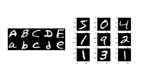
Figure 3: Example of Images from FEMNIST.

Individual Fairness (FEMNIST-skewed, $d=100$) Following the setting in (Li et al. 2018), we first sample 10 lower case characters (‘a’-‘j’) from Extended MNIST (EMNIST) (Cohen et al. 2017) and distribute 5 classes of images to each device. Each local device has 500 images. There are 100 devices in total. Results are reported in Table 2. (FEMNIST-original, $d=500$) Following the setting in (Li et al. 2021), we sample 500 devices and train models using the default data stored in each device. Results are reported in Table 3.

Group Fairness (FEMNIST-3-groups, $d=3$) We manually divide FEMNIST data into three groups. See Table 1 for the detailed assignment. This assignment is inspired by the statistic that most people prefer to write in lowercase letters while a small amount of people use capital letters or a mixed of two types (Jones and Mewhort 2004). In such cases, it is important to assure that an FL algorithm is capable of achieving similar performance between such groups. Results are reported in Table 4.

Group	Data Type	Number of Images	Number of Devices
Group 1	Capital Letters + Digits	800	60
Group 2	Lowercase Letters + Digits	1,000	100
Group 3	Capital/Lowercase Letters + Digits	600	40

Table 1: Data Structure of FEMNIST-3-groups

Implementation: For all tasks, we randomly split the data on each local device into a $70\%$ training set, a $10\%$ validation set and a $20\%$ testing set. This is a common data splitting strategy used in many FL papers (Li et al. 2018, Chen et al. 2018, Reddi et al. 2020). The batch size is set to be 32. We use the tuned initial learning rate $0.1$ and decay rate $0.99$ for each method. During each communication round, $10$ devices are randomly selected and each device will run 2 epochs of SGD. We use a CNN model with 2 convolution layers followed by 2 fully connected layers. All benchmark models are well-tuned. Specifically, we solve q-FFL with $q\in\{0,0.001,0.01,0.1,1,2,5,10\}$ (Li et al. 2019a) in parallel and select the best $q$. Here, the best $q$ is defined as the $q$ value where the variance decreases the most while the averaged testing accuracy is superior or similar to FedAvg. This definition is borrowed from the original q-FFL paper (Li et al. 2019a). Similarly, we train TERM with $t\in\{1,2,5\}$ and select the best $t$ (Li et al. 2020b). For Ditto, we tune the regularization parameter $\lambda_{Ditto}\in\{0.01,0.05,0.1,0.5,1,2,5\}$. In GIFAIR-FL, we tune the parameter $\lambda\in\{0,0.1\lambda_{max},0.2\lambda_{max},\ldots,0.8\lambda_{max},0.9\lambda_{max}\}$. Here kindly note that $\lambda_{max}$ is a function of $p_{k},|{\cal A}_{s_{k}}|$ and $d$ (i.e., data-dependent).

Performance metrics: Denote by $a_{k}$ the prediction accuracy on device $k$. We define (1) individual-level mean accuracy as $\bar{a}\coloneqq\frac{1}{K}\sum_{k=1}^{K}a_{k}$ and (2) individual-level variance as $Var(a)\coloneqq\frac{1}{K}\sum_{k=1}^{K}(a_{k}-\bar{a})^{2}$.

Algorithm	FedAvg	q-FFL	TERM	FedMGDA+	Ditto	GIFAIR-FL-Global	GIFAIR-FL-Per
$\bar{a}$	79.2 (1.0)	84.6 (1.9)	84.2 (1.3)	85.0 (1.7)	92.5 (3.1)	87.9 (0.9)	93.0 (1.1)
$\sqrt{Var(a)}$	22.3 (1.1)	18.5 (1.2)	13.8 (1.0)	14.9 (1.6)	14.3 (1.0)	5.7 (0.8)	6.2 (0.9)

Table 2: Empirical results on FEMNIST-skewed. Each experiment is repeated 5 times.

Algorithm	FedAvg	q-FFL	TERM	AFL	Ditto	GIFAIR-FL-Global	GIFAIR-FL-Per
$\bar{a}$	80.4 (1.3)	80.9 (1.1)	81.0 (1.0)	82.4 (1.0)	83.7 (1.9)	83.2 (0.7)	84.1 (1.2)
$\sqrt{Var(a)}$	11.1 (1.4)	10.6 (1.3)	10.3 (1.2)	9.85 (0.9)	10.1 (1.6)	5.2 (0.8)	4.5 (0.8)

Table 3: Test accuracy on FEMNIST-original. Each experiment is repeated 5 times.

Algorithm	FedAvg	q-FFL	TERM	FedMGDA+	Ditto
Group 1	79.72 (2.08)	81.15 (1.97)	81.29 (1.45)	81.03 (2.28)	82.37 (2.06)
Group 2	90.93 (2.35)	88.24 (2.13)	88.08 (1.09)	89.12 (1.74)	92.05 (2.00)
Group 3	80.21 (2.91)	80.93 (1.86)	81.84 (1.44)	81.33 (1.59)	83.03 (2.18)
Discrepancy	11.21	7.31	6.79	8.09	9.02

Algorithm	GIFAIR-FL-Global	GIFAIR-FL-Per
Group 1	83.41 (1.34)	83.96 (1.22)
Group 2	88.29 (1.22)	91.05 (1.31)
Group 3	84.37 (1.85)	84.98 (0.99)
Discrepancy	6.07	7.09

Table 4: Test accuracy on FEMNIST-3-groups. Each experiment is repeated 5 times. Discrepancy is the difference between the largest accuracy and the smallest accuracy.

5.2 Text Data

Individual Fairness: We train a RNN to predict the next character using text data built from “The Complete Works of William Shakespeare”. In this dataset, there are about 1,129 speaking roles. Naturally, each speaking role in the play is treated as a device. Each device stored several text data and those information will be used to train a RNN on each device. The dataset is available on the LEAF website (Caldas et al. 2018).

Following the setting in McMahan et al. (2017) and Li et al. (2019a), we subsample 31 roles ($d=31$). The RNN model takes a 80-character sequence as the input, and outputs one character after two LSTM layers and one densely-connected layer. For FedAvg, q-FFL and Ditto, the best initial learning rate is 0.8 and decay rate is 0.95 (Li et al. 2021). We also adopt this setting to GIFAIR-FL-Global and GIFAIR-FL-Per. The batch size is set to be 10. The number of local epochs is fixed to be 1 and all models are trained for 500 epochs. Results are reported in Table 5.

Algorithm	FedAvg	q-FFL	AFL	Ditto	GIFAIR-FL-Global	GIFAIR-FL-Per
$\bar{a}$	53.21 (0.31)	53.90 (0.30)	54.58 (0.14)	60.74 (0.42)	57.04 (0.23)	61.58 (0.14)
$\sqrt{Var(a)}$	9.25 (6.17)	7.52 (5.10)	8.44 (5.65)	8.32 (4.77)	3.14 (1.25)	4.33 (1.25)

Table 5: Mean and standard deviation of test accuracy on Shakespeare $(d=31)$. Each experiment is repeated 5 times.

Group Fairness: We obtain the gender information from https://shakespeare.folger.edu/ and group speaking roles based on gender ($d=2$). It is known that the majority of characters in Shakespearean drama are males. Simply training a FedAvg model on this dataset will cause implicit bias towards male characters. On a par with this observation, we subsample 25 males and 10 females from “The Complete Works of William Shakespeare”. Here we note that each device in the male group implicitly has more text data. The setting of hyperparameters is same as that of individual fairness. Results are reported in Table 6.

Algorithm	FedAvg	q-FFL	FedMGDA+	Ditto	GIFAIR-FL-Global	GIFAIR-FL-Per
Male	72.95 (1.70)	67.14 (2.18)	67.07 (2.11)	74.19 (3.75)	67.42(0.98)	73.95 (0.59)
Female	40.39 (1.49)	43.26 (2.05)	43.85 (2.32)	45.73 (4.01)	52.04 (1.10)	54.88 (1.12)
Discrepancy	32.56	23.88	23.22	28.46	15.38	19.07

Table 6: Test accuracy on Shakespeare ($d=2$). Each experiment is repeated 5 times.

5.3 Analysis of Results

Based on Table 2-6, we can obtain important insights. First, compared to other benchmark models, GIFAIR-FL-Global/GIFAIR-FL-Per lead to significantly more fair solutions. As shown in Tables 2, 3 and 5, our algorithm significantly reduces the variance of testing accuracy of all devices (i.e., $Var(a)$) while the average testing accuracy remains consistent. Second, from Tables 4 and 6, it can be seen that GIFAIR-FL-Global/GIFAIR-FL-Per boosted the performance of the group with the worst testing accuracy and achieved the smallest discrepancy. Notably, this boost did not affect the performance of other groups. This indicates that GIFAIR-FL-Global/GIFAIR-FL-Per is capable of ensuring fairness among different groups while retaining a superior or similar prediction accuracy compared to existing benchmark models. Finally, we note that GIFAIR-FL-Global sometimes achieves lower prediction performance than Ditto. This is understandable as Ditto provides a personalized solution to each device $k$ while our model only returns a global parameter $\bm{\bar{\theta}}$. Yet, as shown in the last column, if we use GIFAIR-FL-Per, then the prediction performance can be significantly improved without sacrificing fairness. However, even without personalization, GIFAIR-FL-Global achieves superior testing performance compared to existing fair FL benchmark models.

5.4 Sensitivity Analysis

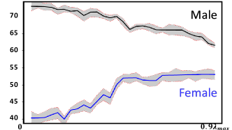
Figure 4: Sensitivity with respect to $\lambda$ (Shakespeare Dataset).

In this section, we use GIFAIR-FL-Global to study the effect of the tuning parameter $\lambda\in[0,\lambda_{max})$ using the Shakespeare dataset. A similar conclusion holds for GIFAIR-FL-Per and we therefore omit it. Results are reported in Figure 4. It can be seen that as $\lambda$ increases, the discrepancy between male and female groups decreases accordingly. However, after $\lambda$ passes a certain threshold, the averaged testing accuracy of the female group remained flat yet the performance of the male group significantly dropped. Therefore, in practice, it is recommended to consider a moderate $\lambda$ value. Intuitively, when $\lambda=0$, GIFAIR-FL becomes FedAvg. When $\lambda$ is close to $\lambda_{max}$, the coefficient (i.e., $(1+\lambda\frac{1}{p_{k}|{\cal A}_{s_{k}}|}r_{k})$) of devices with good performance will be close to zero and the updating is, therefore, impeded. A moderate $\lambda$ balances those two situations well. Besides this example, we also conducted additional sensitivity analysis. Due to space limitation, we defer those results to the Appendix.

6 Conclusion

In this paper, we propose GIFAIR-FL: a framework that imposes group and individual fairness to FL. Experiments show that GIFAIR-FL can lead to more fair solutions compared to recent state-of-the-art fair and personalized FL algorithms while retaining similar testing performance. To the best of our knowledge, fairness in FL is an under underinvestigated area and we hope our work will help inspire continued exploration into fair FL algorithms.

Also, real-life FL datasets for specific engineering or health science applications are still scarce. This is understandable as FL efforts have mainly focused on mobile applications. As such we only test on image classification and text prediction datasets. However, as FL is expected to infiltrate many applications, we hope that more real-life datasets will be generated to provide a means for model validation within different domains. We plan to actively pursue this direction in future research.

Appendix

7 Assumptions

We make the following assumptions. $F_{k}$ is $L$-smooth and $\mu$-strongly convex for all $k\in[K]$.

Denote by $\zeta^{(t)}_{k}$ the batched data from client $k$ and $g_{k}(\bm{\theta}^{(t)}_{k};\zeta^{(t)}_{k})$ the stochastic gradient calculated on this batched data. The variance of stochastic gradients are bounded. Specifically,

$$\mathbb{E}\bigg{\{}\left\lVert g_{k}(\bm{\theta}^{(t)}_{k};\zeta^{(t)}_{k})-\nabla F_{k}(\bm{\theta}^{(t)}_{k})\right\rVert^{2}\bigg{\}}\leq\sigma_{k}^{2},\forall k\in[K].$$

It can be shown that, at local iteration $t$ during communication round $c$,

$$\mathbb{E}\bigg{\{}\left\lVert\nabla H_{k}(\bm{\theta}^{(t)}_{k};\zeta^{(t)}_{k})-\nabla H_{k}(\bm{\theta}^{(t)}_{k})\right\rVert^{2}\bigg{\}}$$

$$=\mathbb{E}\bigg{\{}\left\lVert(1+\frac{\lambda r^{c}_{k}}{p_{k}|{\cal A}_{s_{k}}|})g_{k}(\bm{\theta}^{(t)}_{k};\zeta^{(t)}_{k})-(1+\frac{\lambda r_{k}^{c}}{p_{k}|{\cal A}_{s_{k}}|})\nabla F_{k}(\bm{\theta}^{(t)}_{k})\right\rVert^{2}\bigg{\}}$$

$$\leq(1+\frac{\lambda}{p_{k}|{\cal A}_{s_{k}}|}r_{k}^{c})^{2}\sigma_{k}^{2},\forall k\in[K].$$

Here, $\nabla H_{k}(\bm{\theta}^{(t)}_{k};\zeta^{(t)}_{k})$ denotes the stochastic gradient of $H_{k}$ evaluated on the batched data $\zeta^{(t)}_{k}$. The expected squared norm of stochastic gradient is bounded. Specifically,

$$\mathbb{E}\bigg{\{}\left\lVert g_{k}(\bm{\theta}^{(t)}_{k};\zeta^{(t)}_{k})\right\rVert^{2}\bigg{\}}\leq G^{2},\forall k\in[K].$$

It can be shown that, at local iteration $t$ during communication round $c$,

$$\mathbb{E}\bigg{\{}\left\lVert\nabla H_{k}(\bm{\theta}^{(t)}_{k};\zeta^{(t)}_{k})\right\rVert\bigg{\}}=\mathbb{E}\bigg{\{}\left\lVert(1+\frac{\lambda}{p_{k}|{\cal A}_{s_{k}}|}r_{k}^{c})g_{k}(\bm{\theta}^{(t)}_{k};\zeta^{(t)}_{k})\right\rVert^{2}\bigg{\}}$$

$$\leq(1+\frac{\lambda}{p_{k}|{\cal A}_{s_{k}}|}r_{k}^{c})^{2}G^{2},\forall k\in[K].$$

For the non-convex setting, we replace Assumption 7 by the following assumption. $F_{k}$ is $L$-smooth for all $k\in[K]$. In our proof, for the sake of neatness, we drop the superscript of $r^{c}_{k}$.

We use the definition in Li et al. (2019b) to roughly quantify the degree of non-$i.i.d.$-ness. Specifically,

$$\Gamma_{K}=H^{*}-\sum_{k=1}^{K}p_{k}H^{*}_{k}=\sum_{k=1}^{K}p_{k}(H^{*}-H^{*}_{k}).$$

If data from all sensitive attributes are $i.i.d.$, then $\Gamma_{K}=0$ as number of clients grows. Otherwise, $\Gamma_{K}\neq 0$ (Li et al. 2019b).

8 Detailed Proof

8.1 Proof of Lemma

Lemma 8.1

For any given $\bm{\theta}$, the global objective function $H(\bm{\theta})$ defined in the main paper can be expressed as

$$H(\bm{\theta})=\sum_{k=1}^{K}\left(p_{k}+\dfrac{\lambda}{|{\cal A}_{s_{k}}|}r_{k}(\bm{\theta})\right)F_{k}(\bm{\theta}),$$

where

$$r_{k}(\bm{\theta})\triangleq\sum_{1\leq j\neq s_{k}\leq d}{\mbox{sign}}(L_{s_{k}}(\bm{\theta})-L_{j}(\bm{\theta}))$$

and $s_{k}\in[d]$ is the group index of device $k$. Consequently,

$$H(\bm{\theta})=\sum_{k=1}^{K}\,p_{k}H_{k}(\bm{\theta}).$$

Proof By definition, at communication round $c$,

$$H(\bm{\theta}) =\sum_{k=1}^{K}p_{k}F_{k}(\bm{\theta})+\lambda\sum_{1\leq i<j\leq d}|L_{i}(\bm{\theta})-L_{j}(\bm{\theta})|$$

$$=\sum_{k=1}^{K}p_{k}F_{k}(\bm{\theta})+\lambda\sum_{1\leq i<j\leq d}\bigg{|}\dfrac{1}{|{\cal A}_{i}|}\sum_{k\in{\cal A}_{i}}F_{k}(\bm{\theta})-\dfrac{1}{|{\cal A}_{j}|}\sum_{k\in{\cal A}_{j}}F_{k}(\bm{\theta})\bigg{|}$$

$$=\sum_{k=1}^{K}p_{k}F_{k}(\bm{\theta})+\lambda\sum_{1\leq i<j\leq d}\mbox{sign}(L_{i}(\bm{\theta})-L_{j}(\bm{\theta}))\bigg{(}\dfrac{1}{|{\cal A}_{i}|}\sum_{k\in{\cal A}_{i}}F_{k}(\bm{\theta})-\dfrac{1}{|{\cal A}_{j}|}\sum_{k\in{\cal A}_{j}}F_{k}(\bm{\theta})\bigg{)}$$

$$=\sum_{k=1}^{K}p_{k}F_{k}(\bm{\theta})+\lambda\sum_{u=1}^{d-1}\sum_{u<j\leq d}\mbox{sign}(L_{u}(\bm{\theta})-L_{j}(\bm{\theta}))\bigg{(}\dfrac{1}{|{\cal A}_{u}|}\sum_{k\in{\cal A}_{u}}F_{k}(\bm{\theta})-\dfrac{1}{|{\cal A}_{j}|}\sum_{k\in{\cal A}_{j}}F_{k}(\bm{\theta})\bigg{)}$$

$$=\sum_{k=1}^{K}p_{k}F_{k}(\bm{\theta})+\lambda\sum_{u=1}^{d}\sum_{k\in{\cal A}_{u}}\sum_{u\neq j\leq d}\mbox{sign}(L_{u}(\bm{\theta})-L_{j}(\bm{\theta}))\frac{F_{k}(\bm{\theta})}{|{\cal A}_{u}|}$$

$$=\sum_{k=1}^{K}p_{k}F_{k}(\bm{\theta})+\sum_{k=1}^{K}\frac{\lambda}{|{\cal A}_{s_{k}}|}\sum_{1\leq j\neq s_{k}\leq d}\mbox{sign}(L_{s_{k}}(\bm{\theta})-L_{j}(\bm{\theta}))F_{k}(\bm{\theta})$$

$$=\sum_{k=1}^{K}\left(p_{k}+\dfrac{\lambda}{|{\cal A}_{s_{k}}|}r^{c}_{k}(\bm{\theta})\right)F_{k}(\bm{\theta}).$$

The fifth equality is achieved by rearranging the equation and merging items with the same group label. By definition of $H_{k}$, we thus proved

$$H(\bm{\theta})=\sum_{k=1}^{K}\,p_{k}H_{k}(\bm{\theta}).$$

8.2 Learning Bound

We present a generalization bound for our learning model. Denote by $\mathcal{G}$ the family of the losses associated to a hypothesis set $\mathcal{H}:\mathcal{G}=\{(x,y)\mapsto\ell(h(x),y):h\in\mathcal{H}\}$. The weighted Rademacher complexity (Mohri et al. 2019) is defined as

$$\mathfrak{R}_{\bm{m}}(\mathcal{G},\bm{p})\coloneqq\mathop{\mathbb{E}}_{\bm{\sigma}}\bigg{[}\sup_{h\in\mathcal{H}}\sum_{k=1}^{K}\frac{p_{k}}{N_{k}}\sum_{n=1}^{N_{k}}\sigma_{k,n}\ell(h(x_{k,n}),y_{k,n})\bigg{]}$$

where $\bm{m}=(N_{1},N_{2},\ldots,N_{k})$, $\bm{p}=(p_{1},\ldots,p_{K})$ and $\bm{\sigma}=(\sigma_{k,n})_{k\in[K],n\in[N_{k}]}$ is a collection of Rademacher variables taking values in $\{-1,+1\}$. Denote by $\mathcal{L}_{\mathcal{D}^{\lambda}_{\bm{p}}}(h)$ the expected loss according to our fairness formulation. Denote by $\hat{\mathcal{L}}_{\mathcal{D}^{\lambda}_{\bm{p}}}(h)$ the expected empirical loss (See Appendix for a detailed expression).

Theorem 8.2

Assume that the loss $\ell$ is bounded above by $M>0$. Fix $\epsilon_{0}>0$ and $\bm{m}$. Then, for any $\delta_{0}>0$, with probability at least $1-\delta_{0}$ over samples $D_{k}\sim\mathcal{D}_{k}$, the following holds for all $h\in\mathcal{H}$:

$$\mathcal{L}_{\mathcal{D}^{\lambda}_{\bm{p}}}(h)\leq\hat{\mathcal{L}}_{\mathcal{D}^{\lambda}_{\bm{p}}}(h)+\sqrt{\frac{1}{2}\sum_{k=1}^{K}(\frac{p_{k}}{N_{k}}M+\lambda\frac{d(d-1)}{2}M)^{2}\log\frac{1}{\delta_{0}}}+2\mathfrak{R}_{\bm{m}}(\mathcal{G},\bm{p})+\lambda\frac{d(d-1)}{2}M.$$

It can be seen that, given a sample of data, we can bound the generalization error $\mathcal{L}_{\mathcal{D}^{\lambda}_{\bm{p}}}(h)-\hat{\mathcal{L}}_{\mathcal{D}^{\lambda}_{\bm{p}}}(h)$ with high probability. When $\lambda=0$, the bound is same as the generalization bound in FedAvg (Mohri et al. 2018). When we consider the worst combination of $p_{k}$ by taking the supremum of the upper bound in Theorem 8.2 and let $\lambda=0$, then our generalization bound is same as the one in AFL (Mohri et al. 2019).

Proof Define

$$\Phi(D_{1},\ldots,D_{K})=\sup_{h\in\mathcal{H}}\bigg{(}\mathcal{L}_{\mathcal{D}^{\lambda}_{\bm{p}}}(h)-\hat{\mathcal{L}}_{\mathcal{D}^{\lambda}_{\bm{p}}}(h)\bigg{)}.$$

Let $D^{\prime}=(D_{1}^{\prime},\ldots,D_{K}^{\prime})$ be a sample differing from $D=(D_{1},\ldots,D_{K})$ only by one point $x_{k,n}^{\prime}$. Therefore, we have

$$\Phi(D^{\prime})-\Phi(D) =\sup_{h\in\mathcal{H}}\bigg{(}\mathcal{L}_{\mathcal{D}^{\lambda}_{\bm{p}}}(h)-\hat{\mathcal{L}}_{\mathcal{D}^{{}^{\prime}\lambda}_{\bm{p}}}(h)\bigg{)}-\sup_{h\in\mathcal{H}}\bigg{(}\mathcal{L}_{\mathcal{D}^{\lambda}_{\bm{p}}}(h)-\hat{\mathcal{L}}_{\mathcal{D}^{\lambda}_{\bm{p}}}(h)\bigg{)}$$

$$\leq\sup_{h\in\mathcal{H}}\bigg{(}\mathcal{L}_{\mathcal{D}^{\lambda}_{\bm{p}}}(h)-\hat{\mathcal{L}}_{\mathcal{D}^{{}^{\prime}\lambda}_{\bm{p}}}(h)\bigg{)}-\bigg{(}\mathcal{L}_{\mathcal{D}^{\lambda}_{\bm{p}}}(h)-\hat{\mathcal{L}}_{\mathcal{D}^{\lambda}_{\bm{p}}}(h)\bigg{)}$$

$$\leq\sup_{h\in\mathcal{H}}\big{\{}\sup_{h\in\mathcal{H}}\mathcal{L}_{\mathcal{D}^{\lambda}_{\bm{p}}}(h)-\sup_{h\in\mathcal{H}}\hat{\mathcal{L}}_{\mathcal{D}^{{}^{\prime}\lambda}_{\bm{p}}}(h)-\mathcal{L}_{\mathcal{D}^{\lambda}_{\bm{p}}}(h)+\hat{\mathcal{L}}_{\mathcal{D}^{\lambda}_{\bm{p}}}(h)\big{\}}$$

$$=\sup_{h\in\mathcal{H}}\big{\{}\hat{\mathcal{L}}_{\mathcal{D}^{\lambda}_{\bm{p}}}(h)-\hat{\mathcal{L}}_{\mathcal{D}^{{}^{\prime}\lambda}_{\bm{p}}}(h)\big{\}}$$

By definition,

$$\hat{\mathcal{L}}_{\mathcal{D}^{{}^{\prime}\lambda}_{\bm{p}}}(h) =\sum_{k=1}^{K}\frac{p_{k}}{N_{k}}\sum_{n=1}^{N_{k}}\ell(h(x^{\prime}_{k,n}),y^{\prime}_{k,n})+$$

$$\lambda\sum_{1\leq i<j\leq d}|\frac{\sum_{k\in{\cal A}_{i}}\frac{1}{N_{k}}\sum_{n=1}^{N_{k}}\ell(h(x^{\prime}_{k,n}),y^{\prime}_{k,n})}{|{\cal A}_{i}|}-\frac{\sum_{k\in{\cal A}_{j}}\frac{1}{N_{k}}\sum_{n=1}^{N_{k}}\ell(h(x^{\prime}_{k,n}),y^{\prime}_{k,n})}{|{\cal A}_{j}|}|.$$

Therefore,

$$\sup_{h\in\mathcal{H}}\big{\{}\hat{\mathcal{L}}_{\mathcal{D}^{\lambda}_{\bm{p}}}(h)-\hat{\mathcal{L}}_{\mathcal{D}^{{}^{\prime}\lambda}_{\bm{p}}}(h)\big{\}}$$

$$\leq\sup_{h\in\mathcal{H}}\bigg{[}\frac{p_{k}}{N_{k}}(\ell(h(x^{\prime}_{k,n}),y^{\prime}_{k,n})-\ell(h(x_{k,n}),y_{k,n}))+\lambda\frac{d(d-1)}{2}M\bigg{]}$$

$$\leq\frac{p_{k}}{N_{k}}M+\lambda\frac{d(d-1)}{2}M.$$

By McDiarmid’s inequality, for $\delta_{0}=\exp\bigg{(}\frac{-2\epsilon_{0}^{2}}{\sum_{k=1}^{K}(\frac{p_{k}}{N_{k}}M+\lambda\frac{d(d-1)}{2}M)^{2}}\bigg{)}$, the following holds with probability at least $1-\delta_{0}$

$$\Phi(D)-\mathbb{E}_{D}[\Phi(D)]\leq\epsilon_{0}=\sqrt{\frac{1}{2}\sum_{k=1}^{K}(\frac{p_{k}}{N_{k}}M+\lambda\frac{d(d-1)}{2}M)^{2}\log\frac{1}{\delta_{0}}}.$$

Our next goal is to bound $\mathbb{E}[\Phi(D)]$. We have

$$\mathbb{E}_{D}[\Phi(D)] =\mathbb{E}_{D}\bigg{[}\sup_{h\in\mathcal{H}}\bigg{(}\mathcal{L}_{\mathcal{D}^{\lambda}_{\bm{p}}}(h)-\hat{\mathcal{L}}_{\mathcal{D}^{\lambda}_{\bm{p}}}(h)\bigg{)}\bigg{]}$$

$$=\mathbb{E}_{D}\bigg{[}\sup_{h\in\mathcal{H}}\mathbb{E}_{D^{\prime}}\bigg{(}\hat{\mathcal{L}}_{\mathcal{D}^{{}^{\prime}\lambda}_{\bm{p}}}(h)-\hat{\mathcal{L}}_{\mathcal{D}^{\lambda}_{\bm{p}}}(h)\bigg{)}\bigg{]}$$

$$\leq\mathbb{E}_{D}\mathbb{E}_{D^{\prime}}\sup_{h\in\mathcal{H}}\bigg{(}\hat{\mathcal{L}}_{\mathcal{D}^{{}^{\prime}\lambda}_{\bm{p}}}(h)-\hat{\mathcal{L}}_{\mathcal{D}^{\lambda}_{\bm{p}}}(h)\bigg{)}$$

$$\leq\mathbb{E}_{D}\mathbb{E}_{D^{\prime}}\sup_{h\in\mathcal{H}}\bigg{[}\sum_{k=1}^{K}\frac{p_{k}}{N_{k}}\sum_{n=1}^{N_{k}}\ell(h(x^{\prime}_{k,n}),y^{\prime}_{k,n})-\sum_{k=1}^{K}\frac{p_{k}}{N_{k}}\sum_{n=1}^{N_{k}}\ell(h(x_{k,n}),y_{k,n})+\lambda\frac{d(d-1)}{2}M\bigg{]}$$

$$\leq\mathbb{E}_{D}\mathbb{E}_{D^{\prime}}\mathbb{E}_{\bm{\sigma}}\sup_{h\in\mathcal{H}}\bigg{[}\sum_{k=1}^{K}\frac{p_{k}}{N_{k}}\sum_{n=1}^{N_{k}}\sigma_{k,n}\ell(h(x^{\prime}_{k,n}),y^{\prime}_{k,n})-\sum_{k=1}^{K}\frac{p_{k}}{N_{k}}\sum_{n=1}^{N_{k}}\sigma_{k,n}\ell(h(x_{k,n}),y_{k,n})+\lambda\frac{d(d-1)}{2}M\bigg{]}$$

$$\leq 2\mathfrak{R}_{\bm{m}}(\mathcal{G},\bm{p})+\lambda\frac{d(d-1)}{2}M.$$

Therefore,

$$\Phi(D)\leq\sqrt{\frac{1}{2}\sum_{k=1}^{K}(\frac{p_{k}}{N_{k}}M+\lambda\frac{d(d-1)}{2}M)^{2}\log\frac{1}{\delta_{0}}}+2\mathfrak{R}_{\bm{m}}(\mathcal{G},\bm{p})+\lambda\frac{d(d-1)}{2}M.$$

8.3 Convergence (Strongly Convex)

Our proof is based on the convergence result of FedAvg (Li et al. 2019b).

Theorem 8.3

Assume Assumptions in the main paper hold and $|\mathcal{S}_{c}|=K$. For $\gamma,\mu>0$ and $\eta^{(t)}$ is decreasing in a rate of $\mathcal{O}(\frac{1}{t})$. If $\eta^{(t)}\leq\mathcal{O}(\frac{1}{L})$, we have

$$\mathbb{E}\bigg{\{}H(\bm{\bar{\theta}}^{(T)})\bigg{\}}-H^{*}\leq\frac{L}{2}\frac{1}{\gamma+T}\bigg{\{}\frac{4\xi}{\epsilon^{2}\mu^{2}}+(\gamma+1)\left\lVert\bm{\bar{\theta}}^{(0)}-\bm{\theta}^{*}\right\rVert^{2}\bigg{\}},$$

where $\xi=8(E-1)^{2}G^{2}+4L\Gamma_{K}+2\frac{\Gamma_{max}}{\eta^{(t)}}+4\sum_{k=1}^{K}p_{k}^{2}\sigma_{k}^{2}$ and $\Gamma_{max}\coloneqq\sum_{k=1}^{K}p_{k}|(H^{*}-H^{*}_{k})|\geq|\sum_{k=1}^{K}p_{k}(H^{*}-H^{*}_{k})|=|\Gamma_{K}|$.

Proof

For each device $k$, we introduce an intermediate model parameter $\bm{w}^{(t+1)}_{k}=\bm{\theta}^{(t)}_{k}-\eta^{(t)}\nabla H_{k}(\bm{\theta}^{(t)}_{k})$. If iteration $t+1$ is in the communication round, then $\bm{\theta}^{(t+1)}_{k}=\sum_{k=1}^{K}p_{k}\bm{w}^{(t+1)}_{k}$ (i.e., aggregation). Otherwise, $\bm{\theta}^{(t+1)}_{k}=\bm{w}^{(t+1)}_{k}$. Define $\bm{\bar{w}}^{(t)}=\sum_{k=1}^{K}p_{k}\bm{w}^{(t)}_{k}$ and $\bm{\bar{\theta}}^{(t)}=\sum_{k=1}^{K}p_{k}\bm{\theta}^{(t)}_{k}$. Also, define $\bm{g}^{(t)}=\sum_{k=1}^{K}p_{k}\nabla H_{k}(\bm{\theta}^{(t)}_{k};\zeta^{(t)}_{k})$ and $\bm{\bar{g}}^{(t)}=\mathbb{E}(\bm{g}^{(t)})=\sum_{k=1}^{K}p_{k}\nabla H_{k}(\bm{\theta}^{(t)}_{k})$.

Denote by $\bm{\theta}^{*}$ the optimal model parameter of the global objective function $H(\cdot)$. At iteration $t$, we have

$$\mathbb{E}\bigg{\{}\left\lVert\bm{\bar{\theta}}^{(t+1)}-\bm{\theta}^{*}\right\rVert^{2}\bigg{\}}=\mathbb{E}\bigg{\{}\left\lVert\bm{\bar{\theta}}^{(t)}-\eta^{(t)}\bm{g}^{(t)}-\bm{\theta}^{*}-\eta^{(t)}\bm{\bar{g}}^{(t)}+\eta^{(t)}\bm{\bar{g}}^{(t)}\right\rVert^{2}\bigg{\}}$$

$$=\mathbb{E}\bigg{\{}\left\lVert\bm{\bar{\theta}}^{(t)}-\bm{\theta}^{*}-\eta^{(t)}\bm{\bar{g}}^{(t)}\right\rVert^{2}\bigg{\}}+\mathbb{E}\bigg{\{}2\eta^{(t)}\langle\bm{\bar{\theta}}^{(t)}-\bm{\theta}^{*}-\eta^{(t)}\bm{\bar{g}}^{(t)},\bm{\bar{g}}^{(t)}-\bm{g}^{(t)}\rangle\bigg{\}}+\mathbb{E}\bigg{\{}\eta^{(t)2}\left\lVert\bm{g}^{(t)}-\bm{\bar{g}}^{(t)}\right\rVert^{2}\bigg{\}}$$

$$=\underbrace{\mathbb{E}\bigg{\{}\left\lVert\bm{\bar{\theta}}^{(t)}-\bm{\theta}^{*}-\eta^{(t)}\bm{\bar{g}}^{(t)}\right\rVert^{2}\bigg{\}}}_{A}+\underbrace{\mathbb{E}\bigg{\{}\eta^{(t)2}\left\lVert\bm{g}^{(t)}-\bm{\bar{g}}^{(t)}\right\rVert^{2}\bigg{\}}}_{B},$$

since $\mathbb{E}\bigg{\{}2\eta^{(t)}\langle\bm{\bar{\theta}}^{(t)}-\bm{\theta}^{*}-\eta^{(t)}\bm{\bar{g}}^{(t)},\bm{\bar{g}}^{(t)}-\bm{g}^{(t)}\rangle\bigg{\}}=0$. Our remaining work is to bound term $A$ and term $B$.

Part I: Bounding Term $A$

We can split term $A$ above into three parts:

$$\mathbb{E}\bigg{\{}\left\lVert\bm{\bar{\theta}}^{(t)}-\bm{\theta}^{*}-\eta^{(t)}\bm{\bar{g}}^{(t)}\right\rVert^{2}\bigg{\}}=\mathbb{E}\bigg{\{}\left\lVert\bm{\bar{\theta}}^{(t)}-\bm{\theta}^{*}\right\rVert^{2}\bigg{\}}\underbrace{-2\eta^{(t)}\mathbb{E}\bigg{\{}\langle\bm{\bar{\theta}}^{(t)}-\bm{\theta}^{*},\bm{\bar{g}}^{(t)}\rangle\bigg{\}}}_{\text{C}}+\underbrace{\eta^{(t)2}\mathbb{E}\bigg{\{}\left\lVert\bm{\bar{g}}^{(t)}\right\rVert^{2}\bigg{\}}}_{\text{D}}.$$

For part C, We have

C $$=-2\eta^{(t)}\mathbb{E}\bigg{\{}\langle\bm{\bar{\theta}}^{(t)}-\bm{\theta}^{*},\bm{\bar{g}}^{(t)}\rangle\bigg{\}}=-2\eta^{(t)}\mathbb{E}\bigg{\{}\sum_{k=1}^{K}p_{k}\langle\bm{\bar{\theta}}^{(t)}-\bm{\theta}^{*},\nabla H_{k}(\bm{\theta}_{k}^{(t)})\rangle\bigg{\}}$$

$$=-2\eta^{(t)}\mathbb{E}\bigg{\{}\sum_{k=1}^{K}p_{k}\langle\bm{\bar{\theta}}^{(t)}-\bm{\theta}_{k}^{(t)},\nabla H_{k}(\bm{\theta}_{k}^{(t)})\rangle\bigg{\}}-2\eta^{(t)}\mathbb{E}\bigg{\{}\sum_{k=1}^{K}p_{k}\langle\bm{\theta}_{k}^{(t)}-\bm{\theta}^{*},\nabla H_{k}(\bm{\theta}_{k}^{(t)})\rangle\bigg{\}}$$

To bound C, we need to use Cauchy-Schwarz inequality, inequality of arithmetic and geometric means. Specifically, the Cauchy-Schwarz inequality indicates that

$$\langle\bm{\bar{\theta}}^{(t)}-\bm{\theta}_{k}^{(t)},\nabla H_{k}(\bm{\theta}_{k}^{(t)})\rangle\geq-\left\lVert\bm{\bar{\theta}}^{(t)}-\bm{\theta}_{k}^{(t)}\right\rVert\left\lVert\nabla H_{k}(\bm{\theta}_{k}^{(t)})\right\rVert$$

and inequality of arithmetic and geometric means further implies

$$-\left\lVert\bm{\bar{\theta}}^{(t)}-\bm{\theta}_{k}^{(t)}\right\rVert\left\lVert\nabla H_{k}(\bm{\theta}_{k}^{(t)})\right\rVert\geq-\frac{\left\lVert\bm{\bar{\theta}}^{(t)}-\bm{\theta}_{k}^{(t)}\right\rVert^{2}+\left\lVert\nabla H_{k}(\bm{\theta}_{k}^{(t)})\right\rVert^{2}}{2}.$$

Therefore, we obtain

C $$=-2\eta^{(t)}\mathbb{E}\bigg{\{}\langle\bm{\bar{\theta}}^{(t)}-\bm{\theta}^{*},\bm{\bar{g}}^{(t)}\rangle\bigg{\}}=-2\eta^{(t)}\mathbb{E}\bigg{\{}\sum_{k=1}^{K}p_{k}\langle\bm{\bar{\theta}}^{(t)}-\bm{\theta}^{*},\nabla H_{k}(\bm{\theta}_{k}^{(t)})\rangle\bigg{\}}$$

$$=-2\eta^{(t)}\mathbb{E}\bigg{\{}\sum_{k=1}^{K}p_{k}\langle\bm{\bar{\theta}}^{(t)}-\bm{\theta}_{k}^{(t)},\nabla H_{k}(\bm{\theta}_{k}^{(t)})\rangle\bigg{\}}-2\eta^{(t)}\mathbb{E}\bigg{\{}\sum_{k=1}^{K}p_{k}\langle\bm{\theta}_{k}^{(t)}-\bm{\theta}^{*},\nabla H_{k}(\bm{\theta}_{k}^{(t)})\rangle\bigg{\}}$$

$$\leq\mathbb{E}\bigg{\{}\eta^{(t)}\sum_{k=1}^{K}p_{k}\frac{1}{\eta^{(t)}}\left\lVert\bm{\bar{\theta}}^{(t)}-\bm{\theta}_{k}^{(t)}\right\rVert^{2}+\eta^{(t)^{2}}\sum_{k=1}^{K}p_{k}\left\lVert\nabla H_{k}(\bm{\theta}_{k}^{(t)})\right\rVert^{2}$$

$$\qquad-2\eta^{(t)}\sum_{k=1}^{K}p_{k}(H_{k}(\bm{\theta}_{k}^{(t)})-H_{k}(\bm{\theta}^{*}))-2\eta^{(t)}\sum_{k=1}^{K}p_{k}\frac{(1+\frac{\lambda}{p_{k}|{\cal A}_{s_{k}}|}r_{k}(\bm{\theta}))\mu}{2}\left\lVert\bm{\theta}_{k}^{(t)}-\bm{\theta}^{*}\right\rVert^{2}\bigg{\}},$$

where $-2\eta^{(t)}\mathbb{E}\bigg{\{}\sum_{k=1}^{K}p_{k}\langle\bm{\theta}_{k}^{(t)}-\bm{\theta}^{*},\nabla H_{k}(\bm{\theta}_{k}^{(t)})\rangle\bigg{\}}$ is bounded by the property of strong convexity of $H_{k}$.

Since $H_{k}$ is $(1+\frac{\lambda}{p_{k}|{\cal A}_{s_{k}}|}r_{k}(\bm{\theta}))L$-smooth, we know

$$\left\lVert\nabla H_{k}(\bm{\theta}_{k}^{(t)})\right\rVert^{2}\leq 2(1+\frac{\lambda}{p_{k}|{\cal A}_{s_{k}}|}r_{k}(\bm{\theta}))L(H_{k}(\bm{\theta}_{k}^{(t)})-H_{k}^{*})$$

and therefore

D $$=\eta^{(t)2}\mathbb{E}\bigg{\{}\left\lVert\bm{\bar{g}}^{(t)}\right\rVert^{2}\bigg{\}}\leq\eta^{(t)2}\mathbb{E}\bigg{\{}\sum_{k=1}^{K}p_{k}\left\lVert\nabla H_{k}(\bm{\theta}_{k}^{(t)})\right\rVert^{2}\bigg{\}}$$

$$\leq 2\eta^{(t)2}\mathbb{E}\bigg{\{}\sum_{k=1}^{K}p_{k}(1+\frac{\lambda}{p_{k}|{\cal A}_{s_{k}}|}r_{k}(\bm{\theta}))L(H_{k}(\bm{\theta}_{k}^{(t)})-H_{k}^{*})\bigg{\}}$$

by convexity of norm.

Therefore, combining C and D, we have

$$A =\mathbb{E}\bigg{\{}\left\lVert\bm{\bar{\theta}}^{(t)}-\bm{\theta}^{*}-\eta^{(t)}\bm{\bar{g}}^{(t)}\right\rVert^{2}\bigg{\}}$$

$$\leq\mathbb{E}\bigg{\{}\left\lVert\bm{\bar{\theta}}^{(t)}-\bm{\theta}^{*}\right\rVert^{2}\bigg{\}}+2\eta^{(t)2}\mathbb{E}\bigg{\{}\sum_{k=1}^{K}p_{k}(1+\frac{\lambda}{p_{k}|{\cal A}_{s_{k}}|}r_{k}(\bm{\theta}))L(H_{k}(\bm{\theta}_{k}^{(t)})-H_{k}^{*})\bigg{\}}$$

$$\qquad+\eta^{(t)}\mathbb{E}\bigg{\{}\sum_{k=1}^{K}p_{k}\frac{1}{\eta^{(t)}}\left\lVert\bm{\bar{\theta}}^{(t)}-\bm{\theta}_{k}^{(t)}\right\rVert^{2}\bigg{\}}+\eta^{(t)^{2}}\mathbb{E}\bigg{\{}\sum_{k=1}^{K}p_{k}\left\lVert\nabla H_{k}(\bm{\theta}_{k}^{(t)})\right\rVert^{2}\bigg{\}}$$

$$\qquad-2\eta^{(t)}\mathbb{E}\bigg{\{}\sum_{k=1}^{K}p_{k}(H_{k}(\bm{\theta}_{k}^{(t)})-H_{k}(\bm{\theta}^{*}))\bigg{\}}-2\eta^{(t)}\mathbb{E}\bigg{\{}\sum_{k=1}^{K}p_{k}\frac{(1+\frac{\lambda}{p_{k}|{\cal A}_{s_{k}}|}r_{k}(\bm{\theta}))\mu}{2}\left\lVert\bm{\theta}_{k}^{(t)}-\bm{\theta}^{*}\right\rVert^{2}\bigg{\}}$$

$$\leq\mathbb{E}\bigg{\{}\left\lVert\bm{\bar{\theta}}^{(t)}-\bm{\theta}^{*}\right\rVert^{2}\bigg{\}}-\eta^{(t)}\mathbb{E}\bigg{\{}\sum_{k=1}^{K}p_{k}(1+\frac{\lambda}{p_{k}|{\cal A}_{s_{k}}|}r_{k}(\bm{\theta}))\mu\left\lVert\bm{\theta}_{k}^{(t)}-\bm{\theta}^{*}\right\rVert^{2}\bigg{\}}+\sum_{k=1}^{K}p_{k}\left\lVert\bm{\bar{\theta}}^{(t)}-\bm{\theta}_{k}^{(t)}\right\rVert^{2}$$

$$\qquad+\underbrace{4\eta^{(t)2}\mathbb{E}\bigg{\{}\sum_{k=1}^{K}p_{k}(1+\frac{\lambda}{p_{k}|{\cal A}_{s_{k}}|}r_{k}(\bm{\theta}))L(H_{k}(\bm{\theta}_{k}^{(t)})-H_{k}^{*})\bigg{\}}-2\eta^{(t)}\mathbb{E}\bigg{\{}\sum_{k=1}^{K}p_{k}(H_{k}(\bm{\theta}_{k}^{(t)})-H_{k}(\bm{\theta}^{*}))\bigg{\}}}_{\text{E}}.$$

In the last inequality, we simply rearrange other terms and use the fact that $\left\lVert\nabla H_{k}(\bm{\theta}_{k}^{(t)})\right\rVert^{2}\leq 2(1+\frac{\lambda}{p_{k}|{\cal A}_{s_{k}}|}r_{k}(\bm{\theta}))L(H_{k}(\bm{\theta}_{k}^{(t)})-H_{k}^{*})$ as aforementioned.

To bound E, we define $\gamma^{(t)}_{k}=2\eta^{(t)}(1-2(1+\frac{\lambda}{p_{k}|{\cal A}_{s_{k}}|}r_{k}(\bm{\theta}))L\eta^{(t)})$. Assume $\eta^{(t)}\leq\frac{1}{4(1+\frac{(d-1)}{\min\{p_{k}|{\cal A}_{s_{k}}|\}}\lambda)L}$, then we know $\eta^{(t)}\leq\gamma_{k}^{(t)}\leq 2\eta^{(t)}$.

Therefore, we have

E $$=4\eta^{(t)2}\mathbb{E}\bigg{\{}\sum_{k=1}^{K}p_{k}(1+\frac{\lambda}{p_{k}|{\cal A}_{s_{k}}|}r_{k}(\bm{\theta}))L(H_{k}(\bm{\theta}_{k}^{(t)})-H_{k}^{*})\bigg{\}}-2\eta^{(t)}\mathbb{E}\bigg{\{}\sum_{k=1}^{K}p_{k}(H_{k}(\bm{\theta}_{k}^{(t)})-H_{k}(\bm{\theta}^{*}))\bigg{\}}$$

$$=4\eta^{(t)2}\mathbb{E}\bigg{\{}\sum_{k=1}^{K}p_{k}(1+\frac{\lambda}{p_{k}|{\cal A}_{s_{k}}|}r_{k}(\bm{\theta}))L(H_{k}(\bm{\theta}_{k}^{(t)})-H_{k}^{*})\bigg{\}}-2\eta^{(t)}\mathbb{E}\bigg{\{}\sum_{k=1}^{K}p_{k}(H_{k}(\bm{\theta}_{k}^{(t)})-H_{k}^{*}+H_{k}^{*}-H_{k}(\bm{\theta}^{*}))\bigg{\}}$$

$$=-2\eta^{(t)}\mathbb{E}\bigg{\{}\sum_{k=1}^{K}p_{k}(1-2(1+\frac{\lambda}{p_{k}|{\cal A}_{s_{k}}|}r_{k}(\bm{\theta}))L\eta^{(t)})(H_{k}(\bm{\theta}_{k}^{(t)})-H_{k}^{*})\bigg{\}}+2\eta^{(t)}\mathbb{E}\bigg{\{}\sum_{k=1}^{K}p_{k}(H_{k}(\bm{\theta}^{*})-H_{k}^{*})\bigg{\}}$$

$$=-\mathbb{E}\bigg{\{}\sum_{k=1}^{K}\gamma^{(t)}_{k}p_{k}(H_{k}(\bm{\theta}_{k}^{(t)})-H^{*}+H^{*}-H^{*}_{k})\bigg{\}}+2\eta^{(t)}\mathbb{E}\bigg{\{}H^{*}-\sum_{k=1}^{K}p_{k}H_{k}^{*}\bigg{\}}$$

$$=\underbrace{-\mathbb{E}\bigg{\{}\sum_{k=1}^{K}\gamma_{k}^{(t)}p_{k}(H_{k}(\bm{\theta}_{k}^{(t)})-H^{*})\bigg{\}}}_{\text{F}}+\underbrace{\ \mathbb{E}\bigg{\{}\sum_{k=1}^{K}(2\eta^{(t)}-\gamma_{k}^{(t)})p_{k}(H^{*}-H^{*}_{k})\bigg{\}}}_{\text{G}}.$$

If $H^{*}-H^{*}_{k}\geq 0$ for some $k$, then $(2\eta^{(t)}-\gamma_{k}^{(t)})p_{k}(H^{*}-H^{*}_{k})\leq 2\eta^{(t)}p_{k}(H^{*}-H^{*}_{k})$. If $H^{*}-H^{*}_{k}<0$ otherwise, then $(2\eta^{(t)}-\gamma_{k}^{(t)})p_{k}(H^{*}-H^{*}_{k})$ is negative and $(2\eta^{(t)}-\gamma_{k}^{(t)})p_{k}(H^{*}-H^{*}_{k})\leq-2\eta^{(t)}p_{k}(H^{*}-H^{*}_{k})$. Therefore, by definition of $\Gamma_{max}$,

$$\text{G}\leq 2\eta^{(t)}\mathbb{E}\bigg{\{}\sum_{k=1}^{K}p_{k}|H^{*}-H^{*}_{k}|\bigg{\}}=2\eta^{(t)}\Gamma_{max}.$$

The remaining goal of Part I is to bound term F. Note that

F $$=-\mathbb{E}\bigg{\{}\sum_{k=1}^{K}\gamma_{k}^{(t)}p_{k}(H_{k}(\bm{\theta}_{k}^{(t)})-H^{*})\bigg{\}}$$

$$=-\mathbb{E}\bigg{\{}\bigg{(}\sum_{k=1}^{K}p_{k}\gamma_{k}^{(t)}(H_{k}(\bm{\theta}_{k}^{(t)})-H_{k}(\bm{\bar{\theta}}^{(t)}))+\sum_{k=1}^{K}p_{k}\gamma_{k}^{(t)}(H_{k}(\bm{\bar{\theta}}^{(t)})-H^{*})\bigg{)}\bigg{\}}$$

$$\leq-\mathbb{E}\bigg{\{}\bigg{(}\sum_{k=1}^{K}p_{k}\gamma_{k}^{(t)}\langle\nabla H_{k}(\bm{\bar{\theta}}^{(t)}),\bm{\theta}_{k}^{(t)}-\bm{\bar{\theta}}^{(t)}\rangle+\sum_{k=1}^{K}p_{k}\gamma_{k}^{(t)}(H_{k}(\bm{\bar{\theta}}^{(t)})-H^{*})\bigg{)}\bigg{\}}$$

$$\leq\mathbb{E}\bigg{\{}\sum_{k=1}^{K}\frac{1}{2}\gamma_{k}^{(t)}p_{k}\bigg{[}\eta^{(t)}\left\lVert\nabla H_{k}(\bm{\bar{\theta}}^{(t)})\right\rVert^{2}+\frac{1}{\eta^{(t)}}\left\lVert\bm{\theta}_{k}^{(t)}-\bm{\bar{\theta}}^{(t)}\right\rVert^{2}\bigg{]}-\sum_{k=1}^{K}p_{k}\gamma_{k}^{(t)}(H_{k}(\bm{\bar{\theta}}^{(t)})-H^{*})\bigg{\}}$$

$$\leq\mathbb{E}\bigg{\{}\sum_{k=1}^{K}\gamma_{k}^{(t)}p_{k}\bigg{[}\eta^{(t)}(1+\frac{\lambda}{p_{k}|{\cal A}_{s_{k}}|}r_{k}(\bm{\theta}))L(H_{k}(\bm{\bar{\theta}}^{(t)})-H_{k}^{*})+\frac{1}{2\eta^{(t)}}\left\lVert\bm{\theta}_{k}^{(t)}-\bm{\bar{\theta}}^{(t)}\right\rVert^{2}\bigg{]}$$

$$\qquad-\sum_{k=1}^{K}p_{k}\gamma_{k}^{(t)}(H_{k}(\bm{\bar{\theta}}^{(t)})-H^{*})\bigg{\}}.$$

In the second inequality, we again use the Cauchy–Schwarz inequality and Inequality of arithmetic and geometric means. In the last inequality, we use the fact that $\left\lVert\nabla H_{k}(\bm{\theta}_{k}^{(t)})\right\rVert^{2}\leq 2(1+\frac{\lambda}{p_{k}|{\cal A}_{s_{k}}|}r_{k}(\bm{\theta}))L(H_{k}(\bm{\theta}_{k}^{(t)})-H_{k}^{*})$.

Since $\eta^{(t)}\leq\gamma_{k}^{(t)}\leq 2\eta^{(t)}$, we can bound E as

$$\text{E}\leq\text{F}+\mathbb{E}\bigg{\{}2\eta^{(t)}\Gamma_{max}\bigg{\}}$$

$$=(\eta^{(t)}(1+\frac{\lambda}{p_{k}|{\cal A}_{s_{k}}|}r_{k}(\bm{\theta}))L-1)\mathbb{E}\bigg{\{}\sum_{k=1}^{K}\gamma_{k}^{(t)}p_{k}\bigg{[}(H_{k}(\bm{\bar{\theta}}^{(t)})-H^{*})\bigg{]}\bigg{\}}$$

$$\qquad+\mathbb{E}\bigg{\{}\sum_{k=1}^{K}\eta^{(t)}\gamma_{k}^{(t)}p_{k}(1+\frac{\lambda}{p_{k}|{\cal A}_{s_{k}}|}r_{k}(\bm{\theta}))L(H^{*}-H^{*}_{k})\bigg{\}}$$

$$\qquad+\frac{1}{2\eta^{(t)}}\sum_{k=1}^{K}\gamma_{k}^{(t)}p_{k}\bigg{\{}\left\lVert\bm{\theta}_{k}^{(t)}-\bm{\bar{\theta}}^{(t)}\right\rVert^{2}\bigg{\}}+2\eta^{(t)}\Gamma_{max}$$

$$\leq\mathbb{E}\bigg{\{}\sum_{k=1}^{K}\eta^{(t)}\gamma_{k}^{(t)}p_{k}(1+\frac{\lambda}{p_{k}|{\cal A}_{s_{k}}|}r_{k}(\bm{\theta}))L(H^{*}-H^{*}_{k})\bigg{\}}+\frac{1}{2\eta^{(t)}}\sum_{k=1}^{K}\gamma_{k}^{(t)}p_{k}\mathbb{E}\bigg{\{}\left\lVert\bm{\theta}_{k}^{(t)}-\bm{\bar{\theta}}^{(t)}\right\rVert^{2}\bigg{\}}+2\eta^{(t)}\Gamma_{max}$$

$$\leq\sum_{k=1}^{K}p_{k}\mathbb{E}\bigg{\{}\left\lVert\bm{\theta}_{k}^{(t)}-\bm{\bar{\theta}}^{(t)}\right\rVert^{2}\bigg{\}}+\mathbb{E}\bigg{\{}\sum_{k=1}^{K}\eta^{(t)}\gamma_{k}^{(t)}p_{k}(1+\frac{d-1}{p_{k}|{\cal A}_{s_{k}}|}\lambda)L(H^{*}-H^{*}_{k})\bigg{\}}+2\eta^{(t)}\Gamma_{max}$$

$$\leq\sum_{k=1}^{K}p_{k}\mathbb{E}\bigg{\{}\left\lVert\bm{\theta}_{k}^{(t)}-\bm{\bar{\theta}}^{(t)}\right\rVert^{2}\bigg{\}}+4\eta^{(t)2}L\mathbb{E}\bigg{\{}\sum_{k=1}^{K}p_{k}(H^{*}-H^{*}_{k})\bigg{\}}+2\eta^{(t)}\Gamma_{max}$$

$$=\sum_{k=1}^{K}p_{k}\mathbb{E}\bigg{\{}\left\lVert\bm{\theta}_{k}^{(t)}-\bm{\bar{\theta}}^{(t)}\right\rVert^{2}\bigg{\}}+4\eta^{(t)2}L\Gamma_{K}+2\eta^{(t)}\Gamma_{max}$$

The second inequality holds because $(\eta^{(t)}(1+\frac{\lambda}{p_{k}|{\cal A}_{s_{k}}|}r_{k}(\bm{\theta}))L-1)\leq 0$ and the fourth inequality uses the fact that $1+\frac{d-1}{p_{k}|{\cal A}_{s_{k}}|}\lambda\leq 2$ based on the constraint of $\lambda$.

Therefore,

$$A \leq\mathbb{E}\bigg{\{}\left\lVert\bm{\bar{\theta}}^{(t)}-\bm{\theta}^{*}\right\rVert^{2}\bigg{\}}-\eta^{(t)}\mathbb{E}\bigg{\{}\sum_{k=1}^{K}p_{k}(1+\frac{\lambda}{p_{k}|{\cal A}_{s_{k}}|}r_{k}(\bm{\theta}))\mu\left\lVert\bm{\theta}_{k}^{(t)}-\bm{\theta}^{*}\right\rVert^{2}\bigg{\}}+\sum_{k=1}^{K}p_{k}\left\lVert\bm{\bar{\theta}}^{(t)}-\bm{\theta}_{k}^{(t)}\right\rVert^{2}+\text{E}$$

$$\leq 2\sum_{k=1}^{K}p_{k}\mathbb{E}\bigg{\{}\left\lVert\bm{\bar{\theta}}^{(t)}-\bm{\theta}_{k}^{(t)}\right\rVert^{2}\bigg{\}}+4\eta^{(t)2}L\Gamma_{K}+2\eta^{(t)}\Gamma_{max}+\mathbb{E}\bigg{\{}\left\lVert\bm{\bar{\theta}}^{(t)}-\bm{\theta}^{*}\right\rVert^{2}\bigg{\}}$$

$$\qquad-\eta^{(t)}\mathbb{E}\bigg{\{}\sum_{k=1}^{K}p_{k}(1-\frac{d-1}{p_{k}|{\cal A}_{s_{k}}|}\lambda)\mu\left\lVert\bm{\theta}_{k}^{(t)}-\bm{\theta}^{*}\right\rVert^{2}\bigg{\}}$$

$$\leq 2\sum_{k=1}^{K}p_{k}\mathbb{E}\bigg{\{}\left\lVert\bm{\bar{\theta}}^{(t)}-\bm{\theta}_{k}^{(t)}\right\rVert^{2}\bigg{\}}+4\eta^{(t)2}L\Gamma_{K}+2\eta^{(t)}\Gamma_{max}+\mathbb{E}\bigg{\{}\left\lVert\bm{\bar{\theta}}^{(t)}-\bm{\theta}^{*}\right\rVert^{2}\bigg{\}}$$

$$\qquad-\eta^{(t)}\mathbb{E}\bigg{\{}\sum_{k=1}^{K}p^{2}_{k}(1-\frac{d-1}{p_{k}|{\cal A}_{s_{k}}|}\lambda)\mu\left\lVert\bm{\theta}_{k}^{(t)}-\bm{\theta}^{*}\right\rVert^{2}\bigg{\}}$$

$$\leq 2\sum_{k=1}^{K}p_{k}\mathbb{E}\bigg{\{}\left\lVert\bm{\bar{\theta}}^{(t)}-\bm{\theta}_{k}^{(t)}\right\rVert^{2}\bigg{\}}+4\eta^{(t)2}L\Gamma_{K}+2\eta^{(t)}\Gamma_{max}+\mathbb{E}\bigg{\{}\left\lVert\bm{\bar{\theta}}^{(t)}-\bm{\theta}^{*}\right\rVert^{2}\bigg{\}}$$

$$\qquad-\eta^{(t)}\mathbb{E}\bigg{\{}(1-\frac{d-1}{\min\{p_{k}|{\cal A}_{s_{k}}|\}}\lambda)\mu\frac{1}{K}\left\lVert\sum_{k=1}^{K}p_{k}\bm{\theta}_{k}^{(t)}-\bm{\theta}^{*}\right\rVert^{2}\bigg{\}}$$

$$=2\sum_{k=1}^{K}p_{k}\mathbb{E}\bigg{\{}\left\lVert\bm{\bar{\theta}}^{(t)}-\bm{\theta}_{k}^{(t)}\right\rVert^{2}\bigg{\}}+4\eta^{(t)2}L\Gamma_{K}+2\eta^{(t)}\Gamma_{max}+(1-\eta^{(t)}(1-\frac{d-1}{\min\{p_{k}|{\cal A}_{s_{k}}|\}}\lambda)\frac{\mu}{K})\mathbb{E}\bigg{\{}\left\lVert\bm{\bar{\theta}}^{(t)}-\bm{\theta}^{*}\right\rVert^{2}\bigg{\}}$$

The third inequality uses the fact that $0\leq p_{k}\leq 1$ and $-p_{k}^{2}\geq-p_{k}$. The last inequality uses the fact that $\left\lVert\sum_{k=1}^{K}p_{k}\bm{\theta}_{k}\right\rVert^{2}\leq K\sum_{k=1}^{K}\left\lVert p_{k}\bm{\theta}_{k}\right\rVert^{2}=K\sum_{k=1}^{K}p^{2}_{k}\left\lVert\bm{\theta}_{k}\right\rVert^{2}$ and $1-\frac{d-1}{p_{k}|{\cal A}_{s_{k}}|}\lambda\geq 1-\frac{d-1}{\min\{p_{k}|{\cal A}_{s_{k}}|\}}\lambda$.

Part II: Bounding Term $\sum_{k=1}^{K}p_{k}\mathbb{E}\bigg{\{}\left\lVert\bm{\bar{\theta}}^{(t)}-\bm{\theta}_{k}^{(t)}\right\rVert^{2}\bigg{\}}$ in Term A

For any iteration $t\geq 0$, denote by $t_{0}\leq t$ the index of previous communication iteration before $t$. Since the FL algorithm requires one communication each $E$ steps, we know $t-t_{0}\leq E-1$ and $\bm{\theta}_{k}^{(t_{0})}=\bm{\bar{\theta}}^{(t_{0})}$. Assume $\eta^{(t)}\leq 2\eta^{(t+E)}$. Since $\eta^{(t)}$ is decreasing, we have

$$\mathbb{E}\bigg{\{}\sum_{k=1}^{K}p_{k}\left\lVert\bm{\bar{\theta}}^{(t)}-\bm{\theta}_{k}^{(t)}\right\rVert^{2}\bigg{\}} =\mathbb{E}\bigg{\{}\sum_{k=1}^{K}p_{k}\left\lVert(\bm{\theta}_{k}^{(t)}-\bm{\bar{\theta}}^{(t_{0})})-(\bm{\bar{\theta}}^{(t)}-\bm{\bar{\theta}}^{(t_{0})})\right\rVert^{2}\bigg{\}}$$

$$\leq\mathbb{E}\bigg{\{}\sum_{k=1}^{K}p_{k}\left\lVert\bm{\theta}_{k}^{(t)}-\bm{\bar{\theta}}^{(t_{0})}\right\rVert^{2}\bigg{\}}$$

$$=\mathbb{E}\bigg{\{}\sum_{k=1}^{K}p_{k}\left\lVert\sum_{t=0}^{t-1}\eta^{(t)}g_{k}(\bm{\theta}_{k}^{(t)};\zeta^{(t)}_{k})\right\rVert^{2}\bigg{\}}$$

$$\leq\mathbb{E}\bigg{\{}\sum_{k=1}^{K}p_{k}(t-t_{0})\sum_{t=0}^{t-1}\eta^{(t)2}\left\lVert g_{k}(\bm{\theta}_{k}^{(t)};\zeta^{(t)}_{k})\right\rVert^{2}\bigg{\}}$$

$$\leq\sum_{k=1}^{K}p_{k}\sum_{t=t_{0}}^{t-1}(E-1)\eta^{(t)2}G^{2}\leq\sum_{k=1}^{K}p_{k}\sum_{t=t_{0}}^{t-1}(E-1)\eta^{(t_{0})2}G^{2}$$

$$\leq\sum_{k=1}^{K}p_{k}(E-1)^{2}\eta^{(t_{0})2}G^{2}\leq 4\eta^{(t)2}(E-1)^{2}G^{2}.$$

Part III: Bounding Term B

By assumption, it is easy to show

$$\mathbb{E}\bigg{\{}\eta^{(t)2}\left\lVert\bm{g}^{(t)}-\bm{\bar{g}}^{(t)}\right\rVert^{2}\bigg{\}}\leq\eta^{(t)2}\sum_{k=1}^{K}p_{k}^{2}(1+\frac{\lambda}{p_{k}|{\cal A}_{s_{k}}|}r_{k}(\bm{\theta}))^{2}\sigma_{k}^{2}.$$

Part IV: Proving Convergence

So far, we have shown that

$$\mathbb{E}\bigg{\{}\left\lVert\bm{\bar{\theta}}^{(t+1)}-\bm{\theta}^{*}\right\rVert^{2}\bigg{\}}\leq\text{A}+\text{B}$$

$$\leq 8\eta^{(t)2}(E-1)^{2}G^{2}+4\eta^{(t)2}L\Gamma_{K}+2\eta^{(t)}\Gamma_{max}+(1-\eta^{(t)}(1-\frac{d-1}{p_{k}|{\cal A}_{s_{k}}|}\lambda)\mu)\mathbb{E}\bigg{\{}\left\lVert\bm{\bar{\theta}}^{(t)}-\bm{\theta}^{*}\right\rVert^{2}\bigg{\}}$$

$$\qquad+\eta^{(t)2}\sum_{k=1}^{K}p_{k}^{2}(1+\frac{\lambda}{p_{k}|{\cal A}_{s_{k}}|}r_{k}(\bm{\theta}))^{2}\sigma_{k}^{2}$$

$$=(1-\eta^{(t)}(1-\frac{d-1}{\min\{p_{k}|{\cal A}_{s_{k}}|\}}\lambda)\frac{\mu}{K})\mathbb{E}\bigg{\{}\left\lVert\bm{\bar{\theta}}^{(t)}-\bm{\theta}^{*}\right\rVert^{2}\bigg{\}}+\eta^{(t)^{2}}\xi$$

where $\xi=8(E-1)^{2}G^{2}+4L\Gamma_{K}+2\frac{\Gamma_{max}}{\eta^{(t)}}+\sum_{k=1}^{K}p_{k}^{2}(1+\frac{\lambda}{p_{k}|{\cal A}_{s_{k}}|}r_{k}(\bm{\theta}))^{2}\sigma_{k}^{2}$.

Let $\eta^{(t)}=\frac{\beta}{t+\gamma}$ with $\beta>\frac{1}{(1-\frac{d-1}{min\{p_{k}|{\cal A}_{s_{k}}|\}}\lambda)\frac{\mu}{K}}$ and $\gamma>0$. Define $\epsilon\coloneqq(1-\frac{d-1}{min\{p_{k}|{\cal A}_{s_{k}}|\}}\lambda)$. Let $v=\max\{\frac{\beta^{2}\xi}{\beta\epsilon\mu-1},(\gamma+1)\left\lVert\bm{\bar{\theta}}^{(0)}-\bm{\theta}^{*}\right\rVert^{2}\}$. We will show that $\left\lVert\bm{\bar{\theta}}^{(t)}-\bm{\theta}^{*}\right\rVert^{2}\leq\frac{v}{\gamma+t}$ by induction. For $t=0$, we have $\left\lVert\bm{\bar{\theta}}^{(0)}-\bm{\theta}^{*}\right\rVert^{2}\leq(\gamma+1)\left\lVert\bm{\bar{\theta}}^{(0)}-\bm{\theta}^{*}\right\rVert^{2}\leq\frac{v}{\gamma+1}$. Now assume this is true for some $t$, then

$$\mathbb{E}\bigg{\{}\left\lVert\bm{\bar{\theta}}^{(t+1)}-\bm{\theta}^{*}\right\rVert^{2}\bigg{\}} \leq(1-\eta^{(t)}\epsilon\mu)\mathbb{E}\bigg{\{}\left\lVert\bm{\bar{\theta}}^{(t)}-\bm{\theta}^{*}\right\rVert^{2}\bigg{\}}+\eta^{(t)^{2}}\xi$$

$$\leq(1-\frac{\beta\epsilon\mu}{t+\gamma})\frac{v}{t+\gamma}+\frac{\beta^{2}\xi}{(t+\gamma)^{2}}$$

$$=\frac{t+\gamma-1}{(t+\gamma)^{2}}v+\frac{\beta^{2}\xi}{(t+\gamma)^{2}}-\frac{\beta\epsilon\mu-1}{(t+\gamma)^{2}}v.$$

It is easy to show $\frac{t+\gamma-1}{(t+\gamma)^{2}}v+\frac{\beta^{2}\xi}{(t+\gamma)^{2}}-\frac{\beta\epsilon\mu-1}{(t+\gamma)^{2}}v\leq\frac{v}{t+\gamma+1}$ by definition of $v$. Therefore, we proved $\left\lVert\bm{\bar{\theta}}^{(t)}-\bm{\theta}^{*}\right\rVert^{2}\leq\frac{v}{\gamma+t}$.

By definition, we know $H$ is $\sum_{k=1}^{K}p_{k}\frac{(1+\frac{\lambda}{p_{k}|{\cal A}_{s_{k}}|}r_{k}(\bm{\theta}))}{2}L$-smooth. Therefore,

$$\mathbb{E}\bigg{\{}H(\bm{\bar{\theta}}^{(t)})\bigg{\}}-H^{*} \leq\frac{\sum_{k=1}^{K}p_{k}\frac{(1+\frac{\lambda}{p_{k}|{\cal A}_{s_{k}}|}r_{k}(\bm{\theta}))}{2}L}{2}\mathbb{E}\bigg{\{}\left\lVert\bm{\bar{\theta}}^{(t)}-\bm{\theta}^{*}\right\rVert^{2}\bigg{\}}$$

$$\qquad\leq\frac{\sum_{k=1}^{K}p_{k}\frac{(1+\frac{\lambda}{p_{k}|{\cal A}_{s_{k}}|}r_{k}(\bm{\theta}))}{2}L}{2}\frac{v}{\gamma+t}.$$

By choosing $\beta=\frac{2}{\epsilon\frac{\mu}{K}}$ We have

$$v=\max\{\frac{\beta^{2}\xi}{\beta\epsilon\mu-1},(\gamma+1)\left\lVert\bm{\bar{\theta}}^{(0)}-\bm{\theta}^{*}\right\rVert^{2}\}\leq\frac{\beta^{2}\xi}{\beta\epsilon\mu-1}+(\gamma+1)\left\lVert\bm{\bar{\theta}}^{(0)}-\bm{\theta}^{*}\right\rVert^{2}\leq\frac{4\xi}{\epsilon^{2}\mu^{2}}+(\gamma+1)\left\lVert\bm{\bar{\theta}}^{(0)}-\bm{\theta}^{*}\right\rVert^{2}.$$

Therefore,

$$\mathbb{E}\bigg{\{}H(\bm{\bar{\theta}}^{(T)})\bigg{\}}-H^{*} \leq\frac{\sum_{k=1}^{K}p_{k}\frac{(1+\frac{\lambda}{p_{k}|{\cal A}_{s_{k}}|}r_{k}(\bm{\theta}))}{2}L}{2}\frac{1}{\gamma+T}\bigg{\{}\frac{4\xi}{\epsilon^{2}\mu^{2}}+(\gamma+1)\left\lVert\bm{\bar{\theta}}^{(0)}-\bm{\theta}^{*}\right\rVert^{2}\bigg{\}}$$

$$\leq\frac{\sum_{k=1}^{K}p_{k}\frac{(1+\frac{\lambda(d-1)}{p_{k}|{\cal A}_{s_{k}}|})}{2}L}{2}\frac{1}{\gamma+T}\bigg{\{}\frac{4\xi}{\epsilon^{2}\mu^{2}}+(\gamma+1)\left\lVert\bm{\bar{\theta}}^{(0)}-\bm{\theta}^{*}\right\rVert^{2}\bigg{\}}$$

$$\leq\frac{L}{2}\frac{1}{\gamma+T}\bigg{\{}\frac{4\xi}{\epsilon^{2}\mu^{2}}+(\gamma+1)\left\lVert\bm{\bar{\theta}}^{(0)}-\bm{\theta}^{*}\right\rVert^{2}\bigg{\}}.$$

We thus proved our convergence result.

Theorem 8.4

Assume at each communication round, central server sampled a fraction $\alpha$ of devices and those local devices are sampled according to the sampling probability $p_{k}$. Additionally, assume Assumptions in the main paper hold. For $\gamma,\mu,\epsilon>0$, we have

$$\mathbb{E}\bigg{\{}H(\bm{\bar{\theta}}^{(T)})\bigg{\}}-H^{*}\leq\frac{L}{2}\frac{1}{\gamma+T}\bigg{\{}\frac{4(\xi+\tau)}{\epsilon^{2}\mu^{2}}+(\gamma+1)\left\lVert\bm{\bar{\theta}}^{(0)}-\bm{\theta}^{*}\right\rVert^{2}\bigg{\}},$$

$\tau=\frac{E^{2}}{\left\lceil\alpha K\right\rceil}\sum_{k=1}^{K}p_{k}(1+\frac{\lambda}{p_{k}|{\cal A}_{s_{k}}|}r_{k}(\bm{\theta}))^{2}G^{2}$.

Proof

$$\mathbb{E}\bigg{\{}\left\lVert\bm{\bar{\theta}}^{(t+1)}-\bm{\theta}^{*}\right\rVert^{2}\bigg{\}} =\mathbb{E}\bigg{\{}\left\lVert\bm{\bar{\theta}}^{(t+1)}-\bar{\bm{w}}^{(t+1)}+\bar{\bm{w}}^{(t+1)}-\bm{\theta}^{*}\right\rVert^{2}\bigg{\}}$$

$$=\mathbb{E}\bigg{\{}\left\lVert\bm{\bar{\theta}}^{(t+1)}-\bar{\bm{w}}^{(t+1)}\right\rVert^{2}+\left\lVert\bar{\bm{w}}^{(t+1)}-\bm{\theta}^{*}\right\rVert^{2}+2\langle\bm{\bar{\theta}}^{(t+1)}-\bar{\bm{w}}^{(t+1)},\bar{\bm{w}}^{(t+1)}-\bm{\theta}^{*}\rangle\bigg{\}}$$

$$=\mathbb{E}\bigg{\{}\left\lVert\bm{\bar{\theta}}^{(t+1)}-\bar{\bm{w}}^{(t+1)}\right\rVert^{2}+\left\lVert\bar{\bm{w}}^{(t+1)}-\bm{\theta}^{*}\right\rVert^{2}\bigg{\}}.$$

Note that the expectation is taken over subset $\mathcal{S}_{c}$.

Part I: Bounding Term $\mathbb{E}\bigg{\{}\left\lVert\bm{\bar{\theta}}^{(t+1)}-\bar{\bm{w}}^{(t+1)}\right\rVert^{2}\bigg{\}}$

Assume $\left\lceil\alpha K\right\rceil$ number of local devices are sampled according to sampling probability $p_{k}$. During the communication round, we have $\bar{\bm{\theta}}^{t+1}=\frac{1}{\left\lceil\alpha K\right\rceil}\sum_{l=1}^{\left\lceil\alpha K\right\rceil}\bm{w}^{(t+1)}_{l}$. Therefore,

$$\mathbb{E}\bigg{\{}\left\lVert\bm{\bar{\theta}}^{(t+1)}-\bar{\bm{w}}^{(t+1)}\right\rVert^{2}\bigg{\}} =\mathbb{E}\bigg{\{}\frac{1}{\left\lceil\alpha K\right\rceil^{2}}\left\lVert\sum_{l=1}^{\left\lceil\alpha K\right\rceil}\bm{w}^{(t+1)}_{l}-\bar{\bm{w}}^{(t+1)}\right\rVert^{2}\bigg{\}}$$

$$=\mathbb{E}\bigg{\{}\frac{1}{\left\lceil\alpha K\right\rceil^{2}}\sum_{l=1}^{\left\lceil\alpha K\right\rceil}\left\lVert\bm{w}^{(t+1)}_{l}-\bar{\bm{w}}^{(t+1)}\right\rVert^{2}\bigg{\}}$$

$$=\frac{1}{\left\lceil\alpha K\right\rceil}\sum_{k=1}^{K}p_{k}\left\lVert\bm{w}^{(t+1)}_{k}-\bar{\bm{w}}^{(t+1)}\right\rVert^{2}.$$

We know

$$\sum_{k=1}^{K}p_{k}\left\lVert\bm{w}^{(t+1)}_{k}-\bar{\bm{w}}^{(t+1)}\right\rVert^{2}=\sum_{k=1}^{K}p_{k}\left\lVert(\bm{w}^{(t+1)}_{k}-\bar{\bm{\theta}}^{(t_{0})})-(\bar{\bm{w}}^{(t+1)}-\bar{\bm{\theta}}^{(t_{0})})\right\rVert^{2}\leq\sum_{k=1}^{K}p_{k}\left\lVert(\bm{w}^{(t+1)}_{k}-\bar{\bm{\theta}}^{(t_{0})})\right\rVert^{2},$$

where $t_{0}=t-E+1$. Similarly,

$$\mathbb{E}\bigg{\{}\left\lVert\bm{\bar{\theta}}^{(t+1)}-\bar{\bm{w}}^{(t+1)}\right\rVert^{2}\bigg{\}} \leq\frac{1}{\left\lceil\alpha K\right\rceil}\mathbb{E}\bigg{\{}\sum_{k=1}^{K}p_{k}\left\lVert(\bm{w}^{(t+1)}_{k}-\bar{\bm{\theta}}^{(t_{0})})\right\rVert^{2}\bigg{\}}$$

$$\leq\frac{1}{\left\lceil\alpha K\right\rceil}\mathbb{E}\bigg{\{}\sum_{k=1}^{K}p_{k}\left\lVert(\bm{w}^{(t+1)}_{k}-\bm{\theta}_{k}^{(t_{0})})\right\rVert^{2}\bigg{\}}$$

$$\leq\frac{1}{\left\lceil\alpha K\right\rceil}\mathbb{E}\bigg{\{}\sum_{k=1}^{K}p_{k}E\sum_{m=t_{o}}^{t}\left\lVert\eta^{(m)}\nabla H_{k}(\bm{\theta}_{k}^{(m)};\zeta^{(t)}_{k})\right\rVert^{2}\bigg{\}}$$

$$\leq\frac{E^{2}\eta^{(t_{0})2}}{\left\lceil\alpha K\right\rceil}\sum_{k=1}^{K}p_{k}(1+\frac{\lambda}{p_{k}|{\cal A}_{s_{k}}|}r_{k}(\bm{\theta}))^{2}G^{2}$$

$$\leq\frac{E^{2}\eta^{(t)2}}{\left\lceil\alpha K\right\rceil}\sum_{k=1}^{K}p_{k}(1+\frac{\lambda}{p_{k}|{\cal A}_{s_{k}}|}r_{k}(\bm{\theta}))^{2}G^{2}$$

using the fact that $\eta^{(t)}$ is non-increasing in $t$.

Part II: Convergence Result

As aforementioned,

$$\mathbb{E}\bigg{\{}\left\lVert\bm{\bar{\theta}}^{(t+1)}-\bm{\theta}^{*}\right\rVert^{2}\bigg{\}} =\mathbb{E}\bigg{\{}\left\lVert\bm{\bar{\theta}}^{(t+1)}-\bar{\bm{w}}^{(t+1)}\right\rVert^{2}+\left\lVert\bar{\bm{w}}^{(t+1)}-\bm{\theta}^{*}\right\rVert^{2}\bigg{\}}$$

$$\leq\frac{E^{2}\eta^{(t)2}}{\left\lceil\alpha K\right\rceil}\sum_{k=1}^{K}p_{k}(1+\frac{\lambda}{p_{k}|{\cal A}_{s_{k}}|}r_{k}(\bm{\theta}))^{2}G^{2}+(1-\eta^{(t)}\epsilon\frac{\mu}{K})\mathbb{E}\bigg{\{}\left\lVert\bm{\bar{\theta}}^{(t)}-\bm{\theta}^{*}\right\rVert^{2}\bigg{\}}+\eta^{(t)^{2}}\xi$$

$$=(1-\eta^{(t)}\epsilon\frac{\mu}{K})\mathbb{E}\bigg{\{}\left\lVert\bm{\bar{\theta}}^{(t)}-\bm{\theta}^{*}\right\rVert^{2}\bigg{\}}+\eta^{(t)^{2}}\bigg{(}\xi+\frac{E^{2}}{\left\lceil\alpha K\right\rceil}\sum_{k=1}^{K}p_{k}(1+\frac{\lambda}{p_{k}|{\cal A}_{s_{k}}|}r_{k}(\bm{\theta}))^{2}G^{2}\bigg{)}.$$

Let $\tau=\frac{E^{2}}{\left\lceil\alpha K\right\rceil}\sum_{k=1}^{K}p_{k}(1+\frac{\lambda}{p_{k}|{\cal A}_{s_{k}}|}r_{k}(\bm{\theta}))^{2}G^{2}$. Let $\eta^{(t)}=\frac{\beta}{t+\gamma}$ with $\beta>\frac{1}{\epsilon\frac{\mu}{K}}$ and $\gamma>0$. Let $v=\max\{\frac{\beta^{2}(\xi+\tau)}{\beta\epsilon\mu-1},(\gamma+1)\left\lVert\bm{\bar{\theta}}^{(0)}-\bm{\theta}^{*}\right\rVert^{2}\}$. Similar to the full device participation scenario, we can show that $\mathbb{E}\bigg{\{}\left\lVert\bm{\bar{\theta}}^{(t)}-\bm{\theta}^{*}\right\rVert^{2}\bigg{\}}\leq\frac{v}{\gamma+t}$ by induction.

By definition, we know $H$ is $\sum_{k=1}^{K}p_{k}\frac{(1+\frac{\lambda}{p_{k}|{\cal A}_{s_{k}}|}r_{k}(\bm{\theta}))}{2}L$-smooth. Therefore,

$$\mathbb{E}\bigg{\{}H(\bm{\bar{\theta}}^{(t)})\bigg{\}}-H^{*} \leq\frac{\sum_{k=1}^{K}p_{k}\frac{(1+\frac{\lambda}{p_{k}|{\cal A}_{s_{k}}|}r_{k}(\bm{\theta}))}{2}L}{2}\mathbb{E}\bigg{\{}\left\lVert\bm{\bar{\theta}}^{(t)}-\bm{\theta}^{*}\right\rVert^{2}\bigg{\}}$$

$$\leq\frac{\sum_{k=1}^{K}p_{k}\frac{(1+\frac{\lambda}{p_{k}|{\cal A}_{s_{k}}|}r_{k}(\bm{\theta}))}{2}L}{2}\frac{v}{\gamma+t}.$$

By choosing $\beta=\frac{2}{\epsilon\frac{\mu}{K}}$ We have

$$v=\max\{\frac{\beta^{2}\xi}{\beta\epsilon\mu-1},(\gamma+1)\left\lVert\bm{\bar{\theta}}^{(0)}-\bm{\theta}^{*}\right\rVert^{2}\}\leq\frac{\beta^{2}\xi}{\beta\epsilon\mu-1}+(\gamma+1)\left\lVert\bm{\bar{\theta}}^{(0)}-\bm{\theta}^{*}\right\rVert^{2}\leq\frac{4\xi}{\epsilon^{2}\mu^{2}}+(\gamma+1)\left\lVert\bm{\bar{\theta}}^{(0)}-\bm{\theta}^{*}\right\rVert^{2}.$$

Therefore,

$$\mathbb{E}\bigg{\{}H(\bm{\bar{\theta}}^{(T)})\bigg{\}}-H^{*} \leq\frac{\sum_{k=1}^{K}p_{k}\frac{(1+\frac{\lambda}{p_{k}|{\cal A}_{s_{k}}|}r_{k}(\bm{\theta}))}{2}L}{2}\frac{1}{\gamma+T}\bigg{\{}\frac{4(\xi+\tau)}{\epsilon^{2}\mu^{2}}+(\gamma+1)\left\lVert\bm{\bar{\theta}}^{(0)}-\bm{\theta}^{*}\right\rVert^{2}\bigg{\}}$$

$$\leq\frac{L}{2}\frac{1}{\gamma+T}\bigg{\{}\frac{4(\xi+\tau)}{\epsilon^{2}\mu^{2}}+(\gamma+1)\left\lVert\bm{\bar{\theta}}^{(0)}-\bm{\theta}^{*}\right\rVert^{2}\bigg{\}}$$

8.4 Convergence (Non-convex)

Lemma 8.5

If $\eta^{(t)}\leq\frac{2}{L}$, then $\mathbb{E}\bigg{\{}H(\bm{\bar{\theta}}^{(t)})\bigg{\}}\leq\mathbb{E}\bigg{\{}H(\bm{\bar{\theta}}^{(0)})\bigg{\}}$.

Proof

$$\mathbb{E}\bigg{\{}H(\bm{\bar{\theta}}^{(t+1)})\bigg{\}} =\mathbb{E}\bigg{\{}H(\bm{\bar{\theta}}^{(t)}-\eta^{(t)}\sum_{k=1}^{K}p_{k}\nabla H_{k}(\bm{\theta}^{(t)}_{k};\zeta^{(t)}_{k}))\bigg{\}}$$

$$=\mathbb{E}\bigg{\{}H(\bm{\bar{\theta}}^{(t)}-\eta^{(t)}\sum_{k=1}^{K}p_{k}\nabla H_{k}(\bm{\bar{\theta}}^{(t)};\zeta^{(t)}_{k}))\bigg{\}}$$

$$=\mathbb{E}\bigg{\{}H(\bm{\bar{\theta}}^{(t)}-\eta^{(t)}g^{(t)}(\bm{\bar{\theta}}^{(t)}))\bigg{\}}$$

Here we used the fact that $\bm{\bar{\theta}}^{(t)}=\bm{\theta}^{(t)}_{k}$ since the aggregated model parameter has been distributed to local devices. By Taylor’s theorem, there exists a $\bm{w}^{(t)}$ such that

$$\mathbb{E}\bigg{\{}H(\bm{\bar{\theta}}^{(t+1)})\bigg{\}} =\mathbb{E}\bigg{\{}H(\bm{\bar{\theta}}^{(t)})-\eta^{(t)}g^{(t)}(\bm{\bar{\theta}}^{(t)})^{T}g^{(t)}(\bm{\bar{\theta}}^{(t)})+\frac{1}{2}(\eta^{(t)}g^{(t)}(\bm{\bar{\theta}}^{(t)}))^{T}g^{(t)}(\bm{w}^{(t)})(\eta^{(t)}g^{(t)}(\bm{\bar{\theta}}^{(t)}))\bigg{\}}$$

$$\leq\mathbb{E}\bigg{\{}H(\bm{\bar{\theta}}^{(t)})-\eta^{(t)}g^{(t)}(\bm{\bar{\theta}}^{(t)})^{T}g^{(t)}(\bm{\bar{\theta}}^{(t)})+\eta^{(t)2}\frac{\sum_{k=1}^{K}p_{k}\frac{(1+\frac{\lambda}{p_{k}|{\cal A}_{s_{k}}|}r_{k}(\bm{\theta}))}{2}L}{2}\left\lVert g^{(t)}(\bm{\bar{\theta}}^{(t)}\right\rVert^{2}\bigg{\}}$$

$$\leq\mathbb{E}\bigg{\{}H(\bm{\bar{\theta}}^{(t)})\bigg{\}}-\eta^{(t)}\left\lVert g^{(t)}(\bm{\bar{\theta}}^{(t)}\right\rVert^{2}+\eta^{(t)2}\frac{L}{2}\left\lVert g^{(t)}(\bm{\bar{\theta}}^{(t)}\right\rVert^{2}$$

since $H$ is $\sum_{k=1}^{K}p_{k}\frac{(1+\frac{\lambda}{p_{k}|{\cal A}_{s_{k}}|}r_{k}(\bm{\theta}))}{2}L$-smooth. It can be shown that if $\eta^{(t)}\leq\frac{2}{L}$, we have

$$-\eta^{(t)}\left\lVert g^{(t)}(\bm{\bar{\theta}}^{(t)}\right\rVert^{2}+\eta^{(t)2}\frac{L}{2}\left\lVert g^{(t)}(\bm{\bar{\theta}}^{(t)}\right\rVert^{2}\leq 0.$$

Therefore, By choosing $\eta^{(t)}\leq\frac{2}{L}$, we proved $\mathbb{E}\bigg{\{}H(\bm{\bar{\theta}}^{(t)})\bigg{\}}\leq\mathbb{E}\bigg{\{}H(\bm{\bar{\theta}}^{(0)})\bigg{\}}$.

Theorem 8.6

Assume Assumptions in the main paper hold and $|\mathcal{S}_{c}|=K$. If $\eta^{(t)}=\mathcal{O}(\frac{1}{\sqrt{t}})$ and $\eta^{(t)}\leq\mathcal{O}(\frac{1}{L})$, then for $>0$

$$\min_{t=1,\ldots,T}\mathbb{E}\bigg{\{}\left\lVert\nabla H(\bm{\bar{\theta}}^{(t)})\right\rVert^{2}\bigg{\}}\leq\frac{1}{\sqrt{T}}\bigg{\{}2(1+2KL^{2}\sum_{t=1}^{T}\eta^{(t)2})\mathbb{E}\bigg{\{}H(\bm{\bar{\theta}}^{(0)})-H^{*}\bigg{\}}+2\sum_{t=1}^{T}\xi^{(t)}\bigg{\}},$$

where $\xi^{(t)}=2KL^{2}\eta^{(t)2}\Gamma_{K}+(8\eta^{(t)3}KL^{2}(E-1)+8KL\eta^{(t)2}+4(2+4L)KL\eta^{(t)4}(E-1))G^{2}+(2L\eta^{(t)2}+8KL\eta^{(t)2})\sum_{k=1}^{K}p_{k}\sigma_{k}^{2}$

Proof Since $H$ is $\sum_{k=1}^{K}p_{k}\frac{(1+\frac{\lambda}{p_{k}|{\cal A}_{s_{k}}|}r_{k}(\bm{\theta}))}{2}L$-smooth, we have

$$\mathbb{E}\bigg{\{}H(\bm{\bar{\theta}}^{(t+1)})\bigg{\}} \leq\mathbb{E}\bigg{\{}H(\bm{\bar{\theta}}^{(t)})\bigg{\}}+\underbrace{\mathbb{E}\bigg{\{}\langle\nabla H(\bm{\bar{\theta}}^{(t)}),\bm{\bar{\theta}}^{(t+1)}-\bm{\bar{\theta}}^{(t)}\rangle\bigg{\}}}_{\text{A}}+$$

$$\qquad\frac{\sum_{k=1}^{K}p_{k}\frac{(1+\frac{\lambda}{p_{k}|{\cal A}_{s_{k}}|}r_{k}(\bm{\theta}))}{2}L}{2}\underbrace{\mathbb{E}\bigg{\{}\left\lVert\bm{\bar{\theta}}^{(t+1)}-\bm{\bar{\theta}}^{(t)}\right\rVert^{2}\bigg{\}}}_{\text{B}}.$$

Part I: Bounding Term A

We have

A $$=-\eta^{(t)}\mathbb{E}\bigg{\{}\langle\nabla H(\bm{\bar{\theta}}^{(t)}),\sum_{k=1}^{K}p_{k}\nabla H_{k}(\bm{\theta}_{k}^{(t)};\zeta^{(t)}_{k})\rangle\bigg{\}}=-\eta^{(t)}\mathbb{E}\bigg{\{}\langle\nabla H(\bm{\bar{\theta}}^{(t)}),\sum_{k=1}^{K}p_{k}\nabla H_{k}(\bm{\theta}_{k}^{(t)})\rangle\bigg{\}}$$

$$=-\frac{1}{2}\eta^{(t)}\mathbb{E}\bigg{\{}\left\lVert\nabla H(\bm{\bar{\theta}}^{(t)})\right\rVert^{2}\bigg{\}}-\frac{1}{2}\eta^{(t)}\mathbb{E}\bigg{\{}\left\lVert\sum_{k=1}^{K}p_{k}\nabla H_{k}(\bm{\theta}_{k}^{(t)})\right\rVert^{2}\bigg{\}}+\frac{1}{2}\eta^{(t)}\mathbb{E}\bigg{\{}\left\lVert\nabla H(\bm{\bar{\theta}}^{(t)})-\sum_{k=1}^{K}p_{k}\nabla H_{k}(\bm{\theta}_{k}^{(t)})\right\rVert^{2}\bigg{\}}$$

$$=-\frac{1}{2}\eta^{(t)}\mathbb{E}\bigg{\{}\left\lVert\nabla H(\bm{\bar{\theta}}^{(t)})\right\rVert^{2}\bigg{\}}-\frac{1}{2}\eta^{(t)}\mathbb{E}\bigg{\{}\left\lVert\sum_{k=1}^{K}p_{k}\nabla H_{k}(\bm{\theta}_{k}^{(t)})\right\rVert^{2}\bigg{\}}+\frac{1}{2}\eta^{(t)}\mathbb{E}\bigg{\{}\left\lVert\sum_{k=1}^{K}p_{k}\nabla H_{k}(\bm{\bar{\theta}}^{(t)})-\sum_{k=1}^{K}p_{k}\nabla H_{k}(\bm{\theta}_{k}^{(t)})\right\rVert^{2}\bigg{\}}$$

$$\leq-\frac{1}{2}\eta^{(t)}\mathbb{E}\bigg{\{}\left\lVert\nabla H(\bm{\bar{\theta}}^{(t)})\right\rVert^{2}\bigg{\}}-\frac{1}{2}\eta^{(t)}\mathbb{E}\bigg{\{}\left\lVert\sum_{k=1}^{K}p_{k}\nabla H_{k}(\bm{\theta}_{k}^{(t)})\right\rVert^{2}\bigg{\}}+\frac{1}{2}\eta^{(t)}\mathbb{E}\bigg{\{}K\sum_{k=1}^{K}p_{k}\left\lVert\nabla H_{k}(\bm{\bar{\theta}}^{(t)})-\nabla H_{k}(\bm{\theta}_{k}^{(t)})\right\rVert^{2}\bigg{\}}$$

$$\leq-\frac{1}{2}\eta^{(t)}\mathbb{E}\bigg{\{}\left\lVert\nabla H(\bm{\bar{\theta}}^{(t)})\right\rVert^{2}\bigg{\}}-\frac{1}{2}\eta^{(t)}\mathbb{E}\bigg{\{}\left\lVert\sum_{k=1}^{K}p_{k}\nabla H_{k}(\bm{\theta}_{k}^{(t)})\right\rVert^{2}\bigg{\}}+$$

$$\qquad\frac{1}{2}\eta^{(t)}\mathbb{E}\bigg{\{}K\sum_{k=1}^{K}p_{k}((1+\frac{\lambda}{p_{k}|{\cal A}_{s_{k}}|}r_{k}(\bm{\theta}))L)^{2}\underbrace{\left\lVert\bm{\bar{\theta}}^{(t)}-\bm{\theta}_{k}^{(t)}\right\rVert^{2}}_{\text{C}}\bigg{\}}.$$

In the convex setting, we proved that

$$\text{C}\leq 4\eta^{(t)2}(E-1)G^{2}.$$

This is also true for the non-convex setting since we do not use any property of convex functions.

Part II: Bounding Term B

We have

B $$=\mathbb{E}\bigg{\{}\left\lVert\eta^{(t)}g^{(t)}\right\rVert^{2}\bigg{\}}=\mathbb{E}\bigg{\{}\left\lVert\eta^{(t)}\sum_{k=1}^{K}p_{k}\nabla H_{k}(\bm{\theta}_{k}^{(t)};\zeta^{(t)}_{k})\right\rVert^{2}\bigg{\}}$$

$$=\mathbb{E}\bigg{\{}\left\lVert\eta^{(t)}\sum_{k=1}^{K}p_{k}(\nabla H_{k}(\bm{\theta}_{k}^{(t)};\zeta^{(t)}_{k})-\nabla H_{k}(\bm{\theta}_{k}^{(t)}))\right\rVert^{2}\bigg{\}}+\mathbb{E}\bigg{\{}\left\lVert\eta^{(t)}\sum_{k=1}^{K}p_{k}\nabla H_{k}(\bm{\theta}_{k}^{(t)})\right\rVert^{2}\bigg{\}}$$

$$=\eta^{(t)2}\sum_{k=1}^{K}p_{k}^{2}\mathbb{E}\bigg{\{}\left\lVert\nabla H_{k}(\bm{\theta}_{k}^{(t)};\zeta^{(t)}_{k})-\nabla H_{k}(\bm{\theta}_{k}^{(t)})\right\rVert^{2}\bigg{\}}+\mathbb{E}\bigg{\{}\left\lVert\eta^{(t)}\sum_{k=1}^{K}p_{k}\nabla H_{k}(\bm{\theta}_{k}^{(t)})\right\rVert^{2}\bigg{\}}$$

$$\leq\eta^{(t)2}\sum_{k=1}^{K}p_{k}^{2}(1+\frac{\lambda}{p_{k}|{\cal A}_{s_{k}}|}r_{k}(\bm{\theta}))^{2}\sigma_{k}^{2}+\eta^{(t)2}\mathbb{E}\bigg{\{}K\sum_{k=1}^{K}p_{k}^{2}\left\lVert\nabla H_{k}(\bm{\theta}_{k}^{(t)})\right\rVert^{2}\bigg{\}}.$$

Since $H_{k}$ is $(1+\frac{\lambda}{p_{k}|{\cal A}_{s_{k}}|}r_{k}(\bm{\theta}))L$-smooth, we know

$$\left\lVert\nabla H_{k}(\bm{\theta}_{k}^{(t)})\right\rVert^{2}\leq 2(1+\frac{\lambda}{p_{k}|{\cal A}_{s_{k}}|}r_{k}(\bm{\theta}))L(H_{k}(\bm{\theta}_{k}^{(t)})-H_{k}^{*}).$$

Therefore,

B $$\leq\eta^{(t)2}\sum_{k=1}^{K}p_{k}^{2}(1+\frac{\lambda}{p_{k}|{\cal A}_{s_{k}}|}r_{k}(\bm{\theta}))^{2}\sigma_{k}^{2}+$$

$$\qquad\eta^{(t)2}\mathbb{E}\bigg{\{}K\sum_{k=1}^{K}2p_{k}^{2}(1+\frac{\lambda}{p_{k}|{\cal A}_{s_{k}}|}r_{k}(\bm{\theta}))L(H_{k}(\bm{\theta}_{k}^{(t)})-H_{k}^{*})\bigg{\}}$$

$$=\eta^{(t)2}\sum_{k=1}^{K}p_{k}^{2}(1+\frac{\lambda}{p_{k}|{\cal A}_{s_{k}}|}r_{k}(\bm{\theta}))^{2}\sigma_{k}^{2}+$$

$$\qquad\eta^{(t)2}\mathbb{E}\bigg{\{}K\sum_{k=1}^{K}2p_{k}^{2}(1+\frac{\lambda}{p_{k}|{\cal A}_{s_{k}}|}r_{k}(\bm{\theta}))L(H_{k}(\bm{\theta}_{k}^{(t)})-H^{*}+H^{*}-H_{k}^{*})\bigg{\}}$$

$$\leq\eta^{(t)2}\sum_{k=1}^{K}p_{k}^{2}(1+\frac{\lambda}{p_{k}|{\cal A}_{s_{k}}|}r_{k}(\bm{\theta}))^{2}\sigma_{k}^{2}+$$

$$\qquad\eta^{(t)2}\mathbb{E}\bigg{\{}K\sum_{k=1}^{K}2p_{k}(1+\frac{\lambda}{p_{k}|{\cal A}_{s_{k}}|}r_{k}(\bm{\theta}))L(H_{k}(\bm{\theta}_{k}^{(t)})-H^{*}+H^{*}-H_{k}^{*})\bigg{\}}$$

since $0\leq p_{k}\leq 1$ and $p_{k}^{2}\leq p_{k}$.

Therefore,

$$\mathbb{E}\bigg{\{}H(\bm{\bar{\theta}}^{(t+1)})\bigg{\}} \leq\mathbb{E}\bigg{\{}H(\bm{\bar{\theta}}^{(t)})\bigg{\}}-\frac{1}{2}\eta^{(t)}\mathbb{E}\bigg{\{}\left\lVert\nabla H(\bm{\bar{\theta}}^{(t)})\right\rVert^{2}\bigg{\}}\underbrace{-\frac{1}{2}\eta^{(t)}\mathbb{E}\bigg{\{}\left\lVert\sum_{k=1}^{K}p_{k}\nabla H_{k}(\bm{\theta}_{k}^{(t)})\right\rVert^{2}\bigg{\}}}_{\text{D}<0}+$$

$$\qquad\frac{1}{2}\eta^{(t)}\mathbb{E}\bigg{\{}K\sum_{k=1}^{K}p_{k}((1+\frac{\lambda}{p_{k}|{\cal A}_{s_{k}}|}r_{k}(\bm{\theta}))L)^{2}4\eta^{(t)2}(E-1)G^{2}\bigg{\}}$$

$$\qquad+\frac{\sum_{k=1}^{K}p_{k}\frac{(1+\frac{\lambda}{p_{k}|{\cal A}_{s_{k}}|}r_{k}(\bm{\theta}))}{2}L}{2}\bigg{[}\eta^{(t)2}\sum_{k=1}^{K}p_{k}^{2}(1+\frac{\lambda}{p_{k}|{\cal A}_{s_{k}}|}r_{k}(\bm{\theta}))^{2}\sigma_{k}^{2}$$

$$\qquad+\eta^{(t)2}\mathbb{E}\bigg{\{}K\sum_{k=1}^{K}2p_{k}(1+\frac{\lambda}{p_{k}|{\cal A}_{s_{k}}|}r_{k}(\bm{\theta}))L(H_{k}(\bm{\theta}_{k}^{(t)})-H^{*}+H^{*}-H_{k}^{*})\bigg{\}}\bigg{]}$$

$$\leq\mathbb{E}\bigg{\{}H(\bm{\bar{\theta}}^{(t)})\bigg{\}}-\frac{1}{2}\eta^{(t)}\mathbb{E}\bigg{\{}\left\lVert\nabla H(\bm{\bar{\theta}}^{(t)})\right\rVert^{2}\bigg{\}}$$

$$\qquad\frac{1}{2}\eta^{(t)}\mathbb{E}\bigg{\{}K\sum_{k=1}^{K}p_{k}((1+\frac{\lambda}{p_{k}|{\cal A}_{s_{k}}|}r_{k}(\bm{\theta}))L)^{2}4\eta^{(t)2}(E-1)G^{2}\bigg{\}}$$

$$\qquad+\frac{\sum_{k=1}^{K}p_{k}\frac{(1+\frac{\lambda}{p_{k}|{\cal A}_{s_{k}}|}r_{k}(\bm{\theta}))}{2}L}{2}\bigg{[}\eta^{(t)2}\sum_{k=1}^{K}p_{k}^{2}(1+\frac{\lambda}{p_{k}|{\cal A}_{s_{k}}|}r_{k}(\bm{\theta}))^{2}\sigma_{k}^{2}+$$

$$\qquad\underbrace{4KL\eta^{(t)2}\mathbb{E}\bigg{\{}\sum_{k=1}^{K}p_{k}(H_{k}(\bm{\theta}_{k}^{(t)})-H^{*})+\sum_{k=1}^{K}p_{k}(H^{*}-H_{k}^{*})\bigg{\}}}_{\text{E}}\bigg{]}$$

$$\leq\mathbb{E}\bigg{\{}H(\bm{\bar{\theta}}^{(t)})\bigg{\}}-\frac{1}{2}\eta^{(t)}\mathbb{E}\bigg{\{}\left\lVert\nabla H(\bm{\bar{\theta}}^{(t)})\right\rVert^{2}\bigg{\}}+\frac{1}{2}\eta^{(t)}\mathbb{E}\bigg{\{}K\sum_{k=1}^{K}4p_{k}L^{2}4\eta^{(t)2}(E-1)G^{2}\bigg{\}}$$

$$\qquad+\frac{L}{2}\bigg{[}\eta^{(t)2}\sum_{k=1}^{K}4p_{k}^{2}\sigma_{k}^{2}+\underbrace{4KL\eta^{(t)2}\mathbb{E}\bigg{\{}\sum_{k=1}^{K}p_{k}(H_{k}(\bm{\theta}_{k}^{(t)})-H^{*})+\sum_{k=1}^{K}p_{k}(H^{*}-H_{k}^{*})\bigg{\}}}_{\text{E}}\bigg{]}$$

Here

E $$=4KL\eta^{(t)2}\mathbb{E}\bigg{\{}\sum_{k=1}^{K}p_{k}(H_{k}(\bm{\theta}_{k}^{(t)})-H^{*})\bigg{\}}+4KL\eta^{(t)2}\mathbb{E}\bigg{\{}\sum_{k=1}^{K}p_{k}(H^{*}-H_{k}^{*})\bigg{\}}$$

$$=4KL\eta^{(t)2}\mathbb{E}\bigg{\{}\sum_{k=1}^{K}p_{k}(H_{k}(\bm{\theta}_{k}^{(t)})-H_{k}(\bm{\bar{\theta}}^{(t)}))\bigg{\}}+4KL\eta^{(t)2}\mathbb{E}\bigg{\{}\sum_{k=1}^{K}p_{k}(H_{k}(\bm{\bar{\theta}}^{(t)})-H^{*})\bigg{\}}+4KL\eta^{(t)2}\Gamma_{K}$$

$$=4KL\eta^{(t)2}\underbrace{\mathbb{E}\bigg{\{}\sum_{k=1}^{K}p_{k}(H_{k}(\bm{\theta}_{k}^{(t)})-H_{k}(\bm{\bar{\theta}}^{(t)}))\bigg{\}}}_{\text{F}}+4KL\eta^{(t)2}\mathbb{E}\bigg{\{}H(\bm{\bar{\theta}}^{(t)})-H^{*}\bigg{\}}+4KL\eta^{(t)2}\Gamma_{K}.$$

We can bound term F as

F $$=\mathbb{E}\bigg{\{}\sum_{k=1}^{K}p_{k}(H_{k}(\bm{\theta}_{k}^{(t)})-H_{k}(\bm{\bar{\theta}}^{(t)}))\bigg{\}}$$

$$\leq\mathbb{E}\bigg{\{}\sum_{k=1}^{K}p_{k}(\langle\nabla H_{k}(\bm{\bar{\theta}}^{(t)}),\bm{\theta}_{k}^{(t)}-\bm{\bar{\theta}}^{(t)}\rangle+\frac{(1+\frac{\lambda}{p_{k}|{\cal A}_{s_{k}}|}r_{k}(\bm{\theta}))L}{2}\underbrace{\left\lVert\bm{\theta}_{k}^{(t)}-\bm{\bar{\theta}}^{(t)}\right\rVert^{2}}_{\leq 4\eta^{(t)2}(E-1)G^{2}})\bigg{\}}$$

where we use the fact that $H_{k}$ is $(1+\frac{\lambda}{p_{k}|{\cal A}_{s_{k}}|}r_{k}(\bm{\theta}))L$-smooth. To bound the inner product, we again use the inequality of arithmetic and geometric means and Cauchy–Schwarz inequality:

$$\langle\nabla H_{k}(\bm{\bar{\theta}}^{(t)}),\bm{\theta}_{k}^{(t)}-\bm{\bar{\theta}}^{(t)}\rangle\leq\left\lVert\nabla H_{k}(\bm{\bar{\theta}}^{(t)})\right\rVert\left\lVert\bm{\theta}_{k}^{(t)}-\bm{\bar{\theta}}^{(t)}\right\rVert\leq\frac{\left\lVert\nabla H_{k}(\bm{\bar{\theta}}^{(t)})\right\rVert^{2}+\left\lVert\bm{\theta}_{k}^{(t)}-\bm{\bar{\theta}}^{(t)}\right\rVert^{2}}{2}.$$

It can be shown that

$$\mathbb{E}\bigg{\{}\left\lVert\nabla H_{k}(\bm{\bar{\theta}}^{(t)})\right\rVert^{2}\bigg{\}} =\mathbb{E}\bigg{\{}\left\lVert\nabla F_{k}(\bm{\theta}^{(t)}_{k},D^{(t)}_{k})\right\rVert\bigg{\}}^{2}+\mathbb{E}\bigg{\{}\left\lVert\nabla F_{k}(\bm{\theta}^{(t)}_{k};\zeta^{(t)}_{k})-\nabla F_{k}(\bm{\theta}^{(t)}_{k})\right\rVert^{2}\bigg{\}}$$

$$\leq\mathbb{E}\bigg{\{}\left\lVert\nabla F_{k}(\bm{\theta}^{(t)}_{k};\zeta^{(t)}_{k})\right\rVert^{2}\bigg{\}}+\mathbb{E}\bigg{\{}\left\lVert\nabla F_{k}(\bm{\theta}^{(t)}_{k};\zeta^{(t)}_{k})-\nabla F_{k}(\bm{\theta}^{(t)}_{k})\right\rVert^{2}\bigg{\}}$$

$$\leq(1+\frac{\lambda}{p_{k}|{\cal A}_{s_{k}}|}r_{k}(\bm{\theta}))^{2}(G^{2}+\sigma_{k}^{2})\leq 4(G^{2}+\sigma_{k}^{2})$$

Therefore, we can simplify F as

F $$\leq\mathbb{E}\bigg{\{}\sum_{k=1}^{K}p_{k}(\frac{\left\lVert\nabla H_{k}(\bm{\bar{\theta}}^{(t)})\right\rVert^{2}+\left\lVert\bm{\theta}_{k}^{(t)}-\bm{\bar{\theta}}^{(t)}\right\rVert^{2}}{2}+\frac{(1+\frac{\lambda}{p_{k}|{\cal A}_{s_{k}}|}r_{k}(\bm{\theta}))L}{2}\underbrace{\left\lVert\bm{\theta}_{k}^{(t)}-\bm{\bar{\theta}}^{(t)}\right\rVert^{2}}_{\leq 4\eta^{(t)2}(E-1)G^{2}})\bigg{\}}$$

$$\leq\mathbb{E}\bigg{\{}\sum_{k=1}^{K}p_{k}(\frac{4(G^{2}+\sigma_{k}^{2})+4\eta^{(t)2}(E-1)G^{2}}{2}+4L\eta^{(t)2}(E-1)G^{2})\bigg{\}}$$

$$=2\mathbb{E}\bigg{\{}\sum_{k=1}^{K}p_{k}\sigma_{k}^{2}\bigg{\}}+2G^{2}+(2+4L)\eta^{(t)2}(E-1)G^{2}$$

Combining with E, we obtain

E $$\leq 4KL\eta^{(t)2}\bigg{(}2\sum_{k=1}^{K}p_{k}\sigma_{k}^{2}+2G^{2}+(2+4L)\eta^{(t)2}(E-1)G^{2}\bigg{)}+4KL\eta^{(t)2}\mathbb{E}\bigg{\{}H(\bm{\bar{\theta}}^{(t)})-H^{*}\bigg{\}}+4KL\eta^{(t)2}\Gamma_{K}$$

Part III: Proving Convergence

Therefore,

$$\frac{1}{2}\eta^{(t)}\mathbb{E}\bigg{\{}\left\lVert\nabla H(\bm{\bar{\theta}}^{(t)})\right\rVert^{2}\bigg{\}}$$

$$\leq\mathbb{E}\bigg{\{}H(\bm{\bar{\theta}}^{(t)})\bigg{\}}-\mathbb{E}\bigg{\{}H(\bm{\bar{\theta}}^{(t+1)})\bigg{\}}+\frac{1}{2}\eta^{(t)3}\mathbb{E}\bigg{\{}K\sum_{k=1}^{K}4p_{k}L^{2}4(E-1)G^{2}\bigg{\}}+$$

$$\frac{L}{2}\bigg{[}\eta^{(t)2}\sum_{k=1}^{K}4p_{k}^{2}\sigma_{k}^{2}+4KL\eta^{(t)2}\bigg{(}2\sum_{k=1}^{K}p_{k}\sigma_{k}^{2}+2G^{2}+(2+4L)\eta^{(t)2}(E-1)G^{2}\bigg{)}+4KL\eta^{(t)2}\mathbb{E}\bigg{\{}H(\bm{\bar{\theta}}^{(t)})-H^{*}\bigg{\}}$$

$$\qquad+4KL\eta^{(t)2}\Gamma_{K}\bigg{]}$$

$$=\mathbb{E}\bigg{\{}H(\bm{\bar{\theta}}^{(t)})\bigg{\}}-\mathbb{E}\bigg{\{}H(\bm{\bar{\theta}}^{(t+1)})\bigg{\}}+2KL^{2}\eta^{(t)2}\mathbb{E}\bigg{\{}H(\bm{\bar{\theta}}^{(t)})-H^{*}\bigg{\}}+2KL^{2}\eta^{(t)2}\Gamma_{K}$$

$$\qquad+(8\eta^{(t)3}KL^{2}(E-1)+8KL\eta^{(t)2}+4(2+4L)KL\eta^{(t)4}(E-1))G^{2}+(2L\eta^{(t)2}+8KL\eta^{(t)2})\sum_{k=1}^{K}p_{k}\sigma_{k}^{2}.$$

Let $\xi^{(t)}=2KL^{2}\eta^{(t)2}\Gamma_{K}+(8\eta^{(t)3}KL^{2}(E-1)+8KL\eta^{(t)2}+4(2+4L)KL\eta^{(t)4}(E-1))G^{2}+(2L\eta^{(t)2}+8KL\eta^{(t)2})\sum_{k=1}^{K}p_{k}\sigma_{k}^{2}$, then

$$\frac{1}{2}\eta^{(t)}\mathbb{E}\bigg{\{}\left\lVert\nabla H(\bm{\bar{\theta}}^{(t)})\right\rVert^{2}\bigg{\}} \leq\mathbb{E}\bigg{\{}H(\bm{\bar{\theta}}^{(t)})\bigg{\}}-\mathbb{E}\bigg{\{}H(\bm{\bar{\theta}}^{(t+1)})\bigg{\}}+2KL^{2}\eta^{(t)2}\mathbb{E}\bigg{\{}H(\bm{\bar{\theta}}^{(t)})-H^{*}\bigg{\}}+\xi^{(t)}$$

$$\leq\mathbb{E}\bigg{\{}H(\bm{\bar{\theta}}^{(t)})\bigg{\}}-\mathbb{E}\bigg{\{}H(\bm{\bar{\theta}}^{(t+1)})\bigg{\}}+2KL^{2}\eta^{(t)2}\mathbb{E}\bigg{\{}H(\bm{\bar{\theta}}^{(0)})-H^{*}\bigg{\}}+\xi^{(t)}$$

since $\eta^{(t)}\leq\frac{1}{\sqrt{2K}L}$ and $\mathbb{E}\bigg{\{}H(\bm{\bar{\theta}}^{(t)})\bigg{\}}\leq\mathbb{E}\bigg{\{}H(\bm{\bar{\theta}}^{(0)})\bigg{\}}$ by Lemma 8.5. By taking summation on both side, we obtain

$$\sum_{t=1}^{T}\frac{1}{2}\eta^{(t)}\mathbb{E}\bigg{\{}\left\lVert\nabla H(\bm{\bar{\theta}}^{(t)})\right\rVert^{2}\bigg{\}} \leq\mathbb{E}\bigg{\{}H(\bm{\bar{\theta}}^{(0)})\bigg{\}}-\mathbb{E}\bigg{\{}H(\bm{\bar{\theta}}^{(t+1)})\bigg{\}}+2KL^{2}\sum_{t=1}^{T}\eta^{(t)2}\mathbb{E}\bigg{\{}H(\bm{\bar{\theta}}^{(0)})-H^{*}\bigg{\}}+\sum_{t=1}^{T}\xi^{(t)}$$

$$\leq\mathbb{E}\bigg{\{}H(\bm{\bar{\theta}}^{(0)})\bigg{\}}-\mathbb{E}\bigg{\{}H(\bm{\bar{\theta}}^{*})\bigg{\}}+2KL^{2}\sum_{t=1}^{T}\eta^{(t)2}\mathbb{E}\bigg{\{}H(\bm{\bar{\theta}}^{(0)})-H^{*}\bigg{\}}+\sum_{t=1}^{T}\xi^{(t)}$$

$$=(1+2KL^{2}\sum_{t=1}^{T}\eta^{(t)2})\mathbb{E}\bigg{\{}H(\bm{\bar{\theta}}^{(0)})-H^{*}\bigg{\}}+\sum_{t=1}^{T}\xi^{(t)}.$$

This implies

$$\min_{t=1,\ldots,T}\mathbb{E}\bigg{\{}\left\lVert\nabla H(\bm{\bar{\theta}}^{(t)})\right\rVert^{2}\bigg{\}}\sum_{t=1}^{T}\eta^{(t)}\leq 2(1+2KL^{2}\sum_{t=1}^{T}\eta^{(t)2})\mathbb{E}\bigg{\{}H(\bm{\bar{\theta}}^{(0)})-H^{*}\bigg{\}}+2\sum_{t=1}^{T}\xi^{(t)}$$

and therefore

$$\min_{t=1,\ldots,T}\mathbb{E}\bigg{\{}\left\lVert\nabla H(\bm{\bar{\theta}}^{(t)})\right\rVert^{2}\bigg{\}}\leq\frac{1}{\sum_{t=1}^{T}\eta^{(t)}}\bigg{\{}2(1+2KL^{2}\sum_{t=1}^{T}\eta^{(t)2})\mathbb{E}\bigg{\{}H(\bm{\bar{\theta}}^{(0)})-H^{*}\bigg{\}}+2\sum_{t=1}^{T}\xi^{(t)}\bigg{\}}.$$

Let $\eta^{(t)}=\frac{1}{\sqrt{t}}$, then we have $\sum_{t=1}^{T}\eta^{(t)}=\mathcal{O}(\sqrt{T})$ and $\sum_{t=1}^{T}\eta^{(t)2}=\mathcal{O}(\log(T+1))$. Therefore,

$$\min_{t=1,\ldots,T}\mathbb{E}\bigg{\{}\left\lVert\nabla H(\bm{\bar{\theta}}^{(t)})\right\rVert^{2}\bigg{\}}\leq\frac{1}{\sqrt{T}}\bigg{\{}2(1+2KL^{2}\sum_{t=1}^{T}\eta^{(t)2})\mathbb{E}\bigg{\{}H(\bm{\bar{\theta}}^{(0)})-H^{*}\bigg{\}}+2\sum_{t=1}^{T}\xi^{(t)}\bigg{\}}.$$

9 Additional Experiments

We conduct a sensitivity analysis using the FEMNIST-3-groups setting. Results are reported in Figure 5. Similar to the observation in the main paper, it can be seen that as $\lambda$ increases, the discrepancy between two groups decreases accordingly. Here kindly note that we did not plot group 3 for the sake of neatness. The line of group should stay in the middle of two lines.

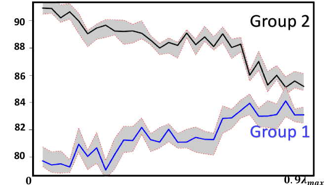
Figure 5: Sensitivity analysis on FEMNIST

References

• Al-Ali et al. (2018) Al-Ali A, Gupta R, Nabulsi AA (2018) Cyber physical systems role in manufacturing technologies. AIP Conference Proceedings, volume 1957, 050007 (AIP Publishing LLC).
• Arivazhagan et al. (2019) Arivazhagan MG, Aggarwal V, Singh AK, Choudhary S (2019) Federated learning with personalization layers. arXiv preprint arXiv:1912.00818 .
• Bhagoji et al. (2019) Bhagoji AN, Chakraborty S, Mittal P, Calo S (2019) Analyzing federated learning through an adversarial lens. International Conference on Machine Learning, 634–643 (PMLR).
• Caldas et al. (2018) Caldas S, Duddu SMK, Wu P, Li T, Konečnỳ J, McMahan HB, Smith V, Talwalkar A (2018) Leaf: A benchmark for federated settings. arXiv preprint arXiv:1812.01097 .
• Chen et al. (2018) Chen F, Luo M, Dong Z, Li Z, He X (2018) Federated meta-learning with fast convergence and efficient communication. arXiv preprint arXiv:1802.07876 .
• CleanTechnica (2021) CleanTechnica (2021) Tesla fsd hardware has 150 million times more computer power than apollo 11 computer. https://cleantechnica.com/2021/05/24/tesla-fsd-hardware-has-150-million-times-more-computer-power-than-apollo-11-computer/, accessed: 2021-05-24.
• Cohen et al. (2017) Cohen G, Afshar S, Tapson J, Van Schaik A (2017) Emnist: Extending mnist to handwritten letters. 2017 International Joint Conference on Neural Networks (IJCNN), 2921–2926 (IEEE).
• Dai et al. (2020) Dai Z, Low KH, Jaillet P (2020) Federated bayesian optimization via thompson sampling. arXiv preprint arXiv:2010.10154 .
• Dinh et al. (2020) Dinh CT, Tran NH, Nguyen TD (2020) Personalized federated learning with moreau envelopes. Conference on Neural Information Processing Systems .
• Du et al. (2020) Du W, Xu D, Wu X, Tong H (2020) Fairness-aware agnostic federated learning. arXiv preprint arXiv:2010.05057 .
• Fallah et al. (2020) Fallah A, Mokhtari A, Ozdaglar A (2020) Personalized federated learning: A meta-learning approach. Advances in Neural Information Processing Systems 33 .
• Feldman et al. (2015) Feldman M, Friedler SA, Moeller J, Scheidegger C, Venkatasubramanian S (2015) Certifying and removing disparate impact. proceedings of the 21th ACM SIGKDD international conference on knowledge discovery and data mining, 259–268.
• Ghosh et al. (2019) Ghosh A, Hong J, Yin D, Ramchandran K (2019) Robust federated learning in a heterogeneous environment. arXiv preprint arXiv:1906.06629 .
• Hard et al. (2018) Hard A, Rao K, Mathews R, Ramaswamy S, Beaufays F, Augenstein S, Eichner H, Kiddon C, Ramage D (2018) Federated learning for mobile keyboard prediction. arXiv preprint arXiv:1811.03604 .
• Hardt et al. (2016) Hardt M, Price E, Srebro N (2016) Equality of opportunity in supervised learning. Conference on Neural Information Processing Systems .
• Hu et al. (2018) Hu B, Gao Y, Liu L, Ma H (2018) Federated region-learning: An edge computing based framework for urban environment sensing. 2018 IEEE Global Communications Conference (GLOBECOM), 1–7 (IEEE).
• Hu et al. (2020) Hu Z, Shaloudegi K, Zhang G, Yu Y (2020) Fedmgda+: Federated learning meets multi-objective optimization. arXiv preprint arXiv:2006.11489 .
• Huang et al. (2020) Huang W, Li T, Wang D, Du S, Zhang J (2020) Fairness and accuracy in federated learning. arXiv preprint arXiv:2012.10069 .
• Jiang et al. (2020) Jiang J, Hu L, Hu C, Liu J, Wang Z (2020) Bacombo—bandwidth-aware decentralized federated learning. Electronics 9(3):440.
• Jiang et al. (2019) Jiang Y, Konečnỳ J, Rush K, Kannan S (2019) Improving federated learning personalization via model agnostic meta learning. arXiv preprint arXiv:1909.12488 .
• Jones and Mewhort (2004) Jones MN, Mewhort DJ (2004) Case-sensitive letter and bigram frequency counts from large-scale english corpora. Behavior research methods, instruments, & computers 36(3):388–396.
• Kairouz et al. (2019) Kairouz P, McMahan HB, Avent B, Bellet A, Bennis M, Bhagoji AN, Bonawitz K, Charles Z, Cormode G, Cummings R, et al. (2019) Advances and open problems in federated learning. arXiv preprint arXiv:1912.04977 .
• Karimireddy et al. (2020) Karimireddy SP, Kale S, Mohri M, Reddi S, Stich S, Suresh AT (2020) Scaffold: Stochastic controlled averaging for federated learning. International Conference on Machine Learning, 5132–5143 (PMLR).
• Khodak et al. (2021) Khodak M, Tu R, Li T, Li L, Balcan MF, Smith V, Talwalkar A (2021) Federated hyperparameter tuning: Challenges, baselines, and connections to weight-sharing. arXiv preprint arXiv:2106.04502 .
• Kontar et al. (2021) Kontar R, Shi N, Yue X, Chung S, Byon E, Chowdhury M, Jin J, Kontar W, Masoud N, Nouiehed M, et al. (2021) The internet of federated things (ioft). IEEE Access 9:156071–156113.
• Li and Wang (2019) Li D, Wang J (2019) Fedmd: Heterogenous federated learning via model distillation. arXiv preprint arXiv:1910.03581 .
• Li et al. (2020a) Li L, Fan Y, Tse M, Lin KY (2020a) A review of applications in federated learning. Computers & Industrial Engineering 106854.
• Li et al. (2020b) Li T, Beirami A, Sanjabi M, Smith V (2020b) Tilted empirical risk minimization. arXiv preprint arXiv:2007.01162 .
• Li et al. (2021) Li T, Hu S, Beirami A, Smith V (2021) Ditto: Fair and robust federated learning through personalization. International Conference on Machine Learning .
• Li et al. (2018) Li T, Sahu AK, Zaheer M, Sanjabi M, Talwalkar A, Smith V (2018) Federated optimization in heterogeneous networks. Conference on Machine Learning and Systems .
• Li et al. (2019a) Li T, Sanjabi M, Beirami A, Smith V (2019a) Fair resource allocation in federated learning. International Conference on Learning Representations .
• Li et al. (2019b) Li X, Huang K, Yang W, Wang S, Zhang Z (2019b) On the convergence of fedavg on non-iid data. arXiv preprint arXiv:1907.02189 .
• Li et al. (2019c) Li X, Yang W, Wang S, Zhang Z (2019c) Communication-efficient local decentralized sgd methods. arXiv preprint arXiv:1910.09126 .
• Liang et al. (2020) Liang PP, Liu T, Ziyin L, Allen NB, Auerbach RP, Brent D, Salakhutdinov R, Morency LP (2020) Think locally, act globally: Federated learning with local and global representations. arXiv preprint arXiv:2001.01523 .
• Lyu et al. (2020) Lyu L, Xu X, Wang Q, Yu H (2020) Collaborative fairness in federated learning. Federated Learning, 189–204 (Springer).
• McMahan et al. (2017) McMahan B, Moore E, Ramage D, Hampson S, y Arcas BA (2017) Communication-efficient learning of deep networks from decentralized data. Artificial Intelligence and Statistics, 1273–1282 (PMLR).
• Mohri et al. (2018) Mohri M, Rostamizadeh A, Talwalkar A (2018) Foundations of machine learning (MIT press).
• Mohri et al. (2019) Mohri M, Sivek G, Suresh AT (2019) Agnostic federated learning. International Conference on Machine Learning, 4615–4625 (PMLR).
• Ramaswamy et al. (2019) Ramaswamy S, Mathews R, Rao K, Beaufays F (2019) Federated learning for emoji prediction in a mobile keyboard. arXiv preprint arXiv:1906.04329 .
• Reddi et al. (2020) Reddi S, Charles Z, Zaheer M, Garrett Z, Rush K, Konečnỳ J, Kumar S, McMahan HB (2020) Adaptive federated optimization. arXiv preprint arXiv:2003.00295 .
• Samsung (2019) Samsung SfB (2019) Your phone is now more powerful than your pc. https://insights.samsung.com/2021/08/19/your-phone-is-now-more-powerful-than-your-pc-3/, accessed: 2019-02-19.
• Sattler et al. (2019) Sattler F, Wiedemann S, Müller KR, Samek W (2019) Robust and communication-efficient federated learning from non-iid data. IEEE transactions on neural networks and learning systems 31(9):3400–3413.
• Smith et al. (2017) Smith V, Chiang CK, Sanjabi M, Talwalkar AS (2017) Federated multi-task learning. Advances in Neural Information Processing Systems, 4424–4434.
• Wang et al. (2020a) Wang H, Sreenivasan K, Rajput S, Vishwakarma H, Agarwal S, Sohn Jy, Lee K, Papailiopoulos D (2020a) Attack of the tails: Yes, you really can backdoor federated learning. Conference on Neural Information Processing Systems .
• Wang et al. (2020b) Wang H, Yurochkin M, Sun Y, Papailiopoulos D, Khazaeni Y (2020b) Federated learning with matched averaging. International Conference on Learning Representations .
• Wang et al. (2019) Wang K, Mathews R, Kiddon C, Eichner H, Beaufays F, Ramage D (2019) Federated evaluation of on-device personalization. arXiv preprint arXiv:1910.10252 .
• Xu and Lyu (2020) Xu X, Lyu L (2020) Towards building a robust and fair federated learning system. arXiv preprint arXiv:2011.10464 .
• Yang et al. (2020) Yang K, Jiang T, Shi Y, Ding Z (2020) Federated learning via over-the-air computation. IEEE Transactions on Wireless Communications 19(3):2022–2035.
• Yu et al. (2020) Yu T, Bagdasaryan E, Shmatikov V (2020) Salvaging federated learning by local adaptation. arXiv preprint arXiv:2002.04758 .
• Yuan and Ma (2020) Yuan H, Ma T (2020) Federated accelerated stochastic gradient descent. Conference on Neural Information Processing Systems .
• Yue and Kontar (2021) Yue X, Kontar RA (2021) Federated gaussian process: Convergence, automatic personalization and multi-fidelity modeling. arXiv preprint arXiv:2111.14008 .
• Zafar et al. (2017) Zafar MB, Valera I, Gomez Rodriguez M, Gummadi KP (2017) Fairness beyond disparate treatment & disparate impact: Learning classification without disparate mistreatment. Proceedings of the 26th international conference on world wide web, 1171–1180.
• Zhang et al. (2020a) Zhang DY, Kou Z, Wang D (2020a) Fairfl: A fair federated learning approach to reducing demographic bias in privacy-sensitive classification models. 2020 IEEE International Conference on Big Data (Big Data), 1051–1060 (IEEE).
• Zhang et al. (2020b) Zhang J, Li C, Robles-Kelly A, Kankanhalli M (2020b) Hierarchically fair federated learning. arXiv preprint arXiv:2004.10386 .
• Zhang et al. (2020c) Zhang X, Zhu X, Wang J, Yan H, Chen H, Bao W (2020c) Federated learning with adaptive communication compression under dynamic bandwidth and unreliable networks. Information Sciences 540:242–262.
• Zhao et al. (2018) Zhao Y, Li M, Lai L, Suda N, Civin D, Chandra V (2018) Federated learning with non-iid data. arXiv preprint arXiv:1806.00582 .