Symmetries in quantum networks lead to no-go theorems for entanglement distribution and to verification techniques

Abstract

Quantum networks are promising tools for the implementation of long-range quantum communication. The characterization of quantum correlations in networks and their usefulness for information processing is therefore central for the progress of the field, but so far only results for small basic network structures or pure quantum states are known. Here we show that symmetries provide a versatile tool for the analysis of correlations in quantum networks. We provide an analytical approach to characterize correlations in large network structures with arbitrary topologies. As examples, we show that entangled quantum states with a bosonic or fermionic symmetry can not be generated in networks; moreover, cluster and graph states are not accessible. Our methods can be used to design certification methods for the functionality of specific links in a network and have implications for the design of future network structures.

I Introduction

A central paradigm for quantum information processing is the notion of quantum networks [1, 2, 3, 4]. In an abstract sense, a quantum network consists of quantum systems as nodes on specific locations, where some of the nodes are connected via links. These links correspond to quantum channels, which may be used to send quantum information (e.g., a polarized photon) or where entanglement may be distributed. Crucial building blocks for the links, such as photonic quantum channels between a satellite and ground stations [5, 6, 7, 8] or the high-rate distribution of entanglement between nodes [9, 10] have recently been experimentally demonstrated. Clearly, such real physical implementations are always noisy and may only work probabilistically, but there are various theoretical approaches to deal with this [12, 13, 14, 11].

For the further progress of the field, it is essential to design methods for the certification and benchmarking of a given network structure or a single specific link within it. In view of current experimental limitations, the question arises which states can be prepared in the network with moderate effort, e.g., with simple local operations. This question has attracted some attention, with several lines of research emerging. First, the problem has been considered in the classical setting, such as the analysis of causal structures [15, 16, 17] or in the study of hidden variable models, where the hidden variables are not equally distributed between every party [18, 19, 20, 21, 22, 23, 24]. Concerning quantum correlations, several initial works appeared in the last year, suggesting slightly different definitions of network entanglement [27, 25, 28, 26]. These have been further investigated [29, 30, 31] and methods from the classical realm have been extended to the quantum scenario [32]. Still, the present results are limited to simple networks like the triangle network, noise-free networks or networks build from specific quantum states, or bounded to small dimensions due to numerical limitations.

In this work, we show an analytical approach to characterize quantum correlations in arbitrary network topologies. Our approach is based on symmetries, which may occur as permutation symmetries or invariance under certain local unitary transformations. Symmetries play an outstanding role in various fields of physics [33] and they have already turned out to be useful for various other problems in quantum information theory [34, 35, 36, 37, 38, 39, 40, 41]. On a technical level, we combine the inflation technique for quantum networks [17, 27] with estimates known from the study of entropic uncertainty relations [44, 43, 42]. Based on our approach, we derive simply testable inequalities in terms of expectation values, which can be used to decide whether a given state may be prepared in a network or not. With this we can prove that large classes of states cannot be prepared in networks using simple communication, for instance all multiparticle graph states with up to twelve vertices with noise, as well as all mixed entangled permutationally symmetric states. This delivers various methods for benchmarking: First, the observation of such states in a network certifies the implementation of advanced network protocols. Second, our results allow to design simple tests for the proper working of a specific link in a given network.

Results

Network entanglement. To start, let us define the types of correlations that can be prepared in a network. In the simplest scenario Alice, Bob and Charlie aim to prepare a tripartite quantum state using three bipartite source states $\varrho_{a}$, $\varrho_{b}$ and $\varrho_{c}$, see Fig. 4. Parties belonging to a same source state are sent to different parties of the network, i.e. $A$, $B$ or $C$, such that the global state reads $\varrho_{ABC}=\varrho_{c}\otimes\varrho_{b}\otimes\varrho_{a}.$ Note that here the order of the parties on both sides of the equation is different. After receiving the states, each party may still apply a local operation $\mathcal{E}_{X}$ (for $X=A,B,C$), in addition these operations may be coordinated by shared randomness. This leads to a global state of the form

$$\varrho=\sum_{\lambda}p_{\lambda}\mathcal{E}_{A}^{(\lambda)}\otimes\mathcal{E}_{B}^{(\lambda)}\otimes\mathcal{E}_{C}^{(\lambda)}\big{[}\varrho_{ABC}\big{]},$$ (1)

and the question arises, which three-party states can be written in this form and which cannot?

Figure 1: Triangle quantum network. Three sources $\varrho_{a}$, $\varrho_{b}$ and $\varrho_{c}$ distribute parties to three nodes, Alice, Bob and Charlie ($A$, $B$ and $C$). The colours yellow, blue and red are associated to the sources $\varrho_{a}$, $\varrho_{b}$ and $\varrho_{c}$ respectively. Alice, Bob and Charlie each end up with a bipartite system $X=X_{1}X_{2}$ on which they perform a local channel $\mathcal{E}_{X}^{(\lambda)}$ ($X=A,B,C$) depending on a classical random variable $\lambda$.

Some remarks are in order: First, the definition of network states in Eq. (1) can directly be extended to more parties or more advanced sources, e.g. one can consider the case of five parties $A,B,C,D,E,$ where some sources distribute four-party states between some of the parties. Second, the scenario considered uses local operations and shared randomness (LOSR) as allowed operations, which is a smaller set than local operations and classical communication (LOCC). In fact, LOCC are much more difficult to implement, but using LOCC and teleportation any tripartite state can be prepared from bipartite sources. On the other hand, the set LOSR is strictly larger than, e.g., the unitary operations considered in refs. [26, 25]. Finally, the discerning reader may have noticed that in Eq. (1) the state $\varrho_{ABC}$ does not depend on the shared random variable $\lambda$, but since the dimension of the source states $\varrho_{i}$ is not bounded one can always remove a dependency on $\lambda$ in the $\varrho_{i}$ by enlarging the dimension [27]. Equivalently, one may remove the dependency of the maps $\mathcal{E}_{X}$ on $\lambda$ and the shared randomness may be carried by the source states only.

Symmetries. Symmetry groups can act on quantum states in different ways. First, the elements of a unitary symmetry group may act transitively on the density matrix $\varrho$. That is, $\varrho$ is invariant under transformations like

$$\varrho\longmapsto U\varrho U^{\dagger}=\varrho.$$ (2)

If $\varrho=|\psi\rangle\langle\psi|$ is pure, this implies $U|\psi\rangle=e^{i\phi}|\psi\rangle$ and $|\psi\rangle$ is, up to some phase, an eigenstate of some operator. Second, for pure states one can also identify directly a certain subspace of the entire Hilbert space that is equipped with a certain symmetry, e.g. symmetry under exchange of two particles. Denoting by $\Pi$ the projector onto this subspace, the symmetric pure states are defined via

$$\Pi|\psi\rangle=|\psi\rangle$$ (3)

and for mixed states one has $\varrho=\Pi\varrho\Pi$. Note that if $\varrho=\sum_{k}p_{k}|\phi_{k}\rangle\langle\phi_{k}|$ has some decomposition into pure states, then each $|\phi_{k}\rangle=\Pi|\phi_{k}\rangle$ has to be symmetric, too.

In the following, we consider mainly two types of symmetries. First, we consider multi-qubit states obeying a symmetry as in Eq. (2) where the symmetry operations consist of an Abelian group of tensor products of Pauli matrices. These groups are usually referred to as stabilizers in quantum information theory [45], and they play a central role in the construction of quantum error correcting codes. Pure states obeying such symmetries are also called stabilizer states, or, equivalently, graph states [46, 47]. Second, we consider states with a permutational (or bosonic) symmetry [36, 39, 48], obeying relations as in Eq. (3) with $\Pi$ being the projector onto the symmetric subspace.

GHZ states. As a warming-up exercise we discuss the Greenberger-Horne-Zeilinger (GHZ) state of three qubits,

$$|GHZ\rangle=\frac{1}{\sqrt{2}}(|000\rangle+|111\rangle)$$ (4)

in the triangle scenario. This simple case was already the main example in previous works on network correlations [27, 25, 26], but it allows us to introduce our concepts and ideas in a simple setting, such that their full generalization is later conceivable.

The GHZ state is an eigenstate of the observables

$$g_{1}=X_{A}X_{B}X_{C},\quad g_{2}=1_{A}Z_{B}Z_{C},\quad g_{3}=Z_{A}Z_{B}1_{C}.$$ (5)

Here and in the following we use the shorthand notation $1_{A}X_{B}Y_{C}=\mathds{1}\otimes\sigma_{x}\otimes\sigma_{y}$ for tensor products of Pauli matrices. Indeed, these $g_{k}$ commute and generate the stabilizer $\mathcal{S}=\{\mathds{1},g_{1},g_{2},g_{3},g_{1}g_{2},g_{1}g_{3},g_{2}g_{3},g_{1}g_{2}g_{3}\}$. Clearly, for any $S_{i}\in\mathcal{S}$ we have $S_{i}|GHZ\rangle=|GHZ\rangle$ and so $\langle GHZ|S_{i}|GHZ\rangle=1$.

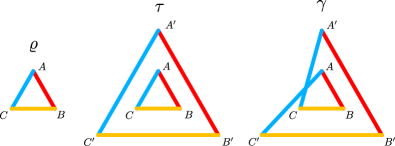
Figure 2: Triangle network and two of its inflations. The first figure represents the triangle network of Fig. 4, with global state $\varrho$ and parties $A$, $B$ and $C$. Using the same source states (represented by lines of same colour, i.e. yellow, blue and red are associated to the sources $\varrho_{a}$, $\varrho_{b}$ and $\varrho_{c}$ of Fig. 4 respectively) and same local channels, one can build the so-called inflated state $\tau$ with parties $X$, $X^{\prime}$ ($X=A,B,C$). This state is separable with respect to the $ABC|A^{\prime}B^{\prime}C^{\prime}$ partition. The state $\gamma$ is build similarly, but with a rewiring of the sources, leading to an inflated state that is in general not separable and different from $\tau$. Still, this procedure imposes that several marginals of $\varrho$, $\tau$ and $\gamma$ are equal, e.g. $\varrho_{AC}=\tau_{A^{\prime}C^{\prime}}=\gamma_{A^{\prime}C}$. The parties of $\gamma$ are labeled in the same way than $\tau$. Note that this is a simplified version of Fig. 4, i.e. that the local channels and the randomness source are not depicted but implied.

As a tool for studying network entanglement, we use the inflation technique [17, 32]. The basic idea is depicted in Fig. (2). If a state $\varrho$ can be prepared in the network scenario, then one can also consider a scenario where each source state is sent two-times to multiple copies of the parties. In this multicopy scenario, the source states may, however, also be wired in a different manner. In the simplest case of doubled sources, this may lead to two different states, $\tau$ and $\gamma$. Although $\varrho$, $\tau$ and $\gamma$ are different states, some of their marginals are identical, see Fig. (2) and Supplementary Note 1. If one can prove that states $\tau$ and $\gamma$ with the marginal conditions do not exist, then $\varrho$ cannot be prepared in the network.

Let us start by considering the correlation $\left\langle Z_{A}Z_{B}\right\rangle$ in $\varrho$, $\tau$ and $\gamma$. The values are equal in all three states, $\left\langle Z_{A}Z_{B}\right\rangle_{\varrho}=\left\langle Z_{A}Z_{B}\right\rangle_{\tau}=\left\langle Z_{A}Z_{B}\right\rangle_{\gamma}$, and the same holds for the correlation $\left\langle Z_{B}Z_{C}\right\rangle.$ Note that these should be large, if $\varrho$ is close to a GHZ state, as $Z_{A}Z_{B}$ is an element of the stabilizer. Using the general relation $\left\langle Z_{A}Z_{C}\right\rangle\geq\left\langle Z_{A}Z_{B}\right\rangle+\left\langle Z_{B}Z_{C}\right\rangle-1$ [27] we can use this to estimate $\left\langle Z_{A}Z_{C}\right\rangle$ in $\gamma$. Due to the marginal conditions, we have $\left\langle Z_{A}Z_{C}\right\rangle_{\gamma}=\left\langle Z_{A^{\prime}}Z_{C}\right\rangle_{\tau}$, implying that this correlation in $\tau$ must be large, if $\varrho$ is close to a GHZ state. On the other hand, the correlation $\left\langle X_{A}X_{B}X_{C}\right\rangle$ corresponds also to a stabilizer element and should be large in the state $\varrho$ as well as in $\tau$.

The key observation is that the observables $X_{A}X_{B}X_{C}$ and $Z_{A^{\prime}}Z_{C}$ anticommute; moreover, they have only eigenvalues $\pm 1$. For this situation, strong constraints on the expectation values are known: If $M_{i}$ are pairwise anticommuting observables with eigenvalues $\pm 1$, then $\sum_{i}\left\langle M_{i}\right\rangle^{2}\leq 1$ [44]. This fact has already been used to derive entropic uncertainty relations [42, 43] or monogamy relations [49, 50]. For our situation, it directly implies that for $\tau$ the correlations $\left\langle X_{A}X_{B}X_{C}\right\rangle$ and $\left\langle Z_{A^{\prime}}Z_{C}\right\rangle$ cannot both be large. Or, expressing everything in terms of the original state $\varrho$, if $\left\langle Z_{A}Z_{B}\right\rangle+\left\langle Z_{B}Z_{C}\right\rangle-1\geq 0$ then a condition for preparability of a state in the network is

$$\left\langle X_{A}X_{B}X_{C}\right\rangle^{2}+(\left\langle Z_{A}Z_{B}\right\rangle+\left\langle Z_{B}Z_{C}\right\rangle-1)^{2}\leq 1.$$ (6)

This is clearly violated by the GHZ state. In fact, if one considers a GHZ state mixed with white noise, $\varrho=p|GHZ\rangle\langle GHZ|+(1-p)\mathds{1}/8$, then these states are detected already for $p>4/5.$ Note that using the other observables of the stabilizer and permutations of the particles, also other conditions like $\left\langle Y_{A}Y_{B}X_{C}\right\rangle^{2}+(\left\langle Z_{A}Z_{B}\right\rangle+\left\langle Z_{A}Z_{C}\right\rangle-1)^{2}\leq 1$ can be derived.

Using these techniques as well as concepts based on covariance matrices [28, 29] and classical networks [23], one can also derive bounds on the maximal GHZ fidelity achievable by network states. In fact, for network states

$$F_{GHZ}=\langle GHZ|\varrho|GHZ\rangle\leq\frac{1}{\sqrt{2}}\approx 0.7071$$ (7)

holds, as explained in Supplementary Note 2. This is a clear improvement on previous analytical bounds, although it does not improve a fidelity bound obtained by numerical convex optimization [27].

Cluster and graph states. The core advantage of our approach is the fact that it can directly be generalized to more parties and complicated networks, while the existing numerical and analytical approaches are mostly restricted to the triangle scenario.

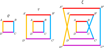
Figure 3: Square network and two of its inflations. Similar to the triangle network of Fig. 2, the state $\tau$ is generated using two copies of the sources and channels used to generate $\varrho$. Then, one goes to a higher-order inflation by using three copies of the sources and the local channels. By rewiring one obtains the inflated state $\xi$. Again, one has several equalities between the marginals of $\varrho$, $\tau$ and $\xi$. Parties with a link of same colour are connected by an identical source, as in Fig. 2. The labels $X$, $X^{\prime}$, $X^{\prime\prime}$ ($X=A,B,C$) denote the parties of the states.

Let us start the discussion with the four-qubit cluster state $|C_{4}\rangle.$ This may be defined as the unique common $+1$-eigenstate of

$$g_{1} =X_{A}Z_{B}1_{C}Z_{D},\ g_{2}=Z_{A}X_{B}Z_{C}1_{D},$$

$$g_{3} =1_{A}Z_{B}X_{C}Z_{D},\ g_{4}=Z_{A}1_{B}Z_{C}X_{D}.$$ (8)

For later generalization, it is useful to note that the choice of these observables is motivated by a graphical analogy. For the square graph in Fig. 3 one can associate to any vertex a stabilizing operator in the following manner: One takes $X$ on the vertex $i$, and $Z$ on its neighbours, i.e. the vertices connected to $i$. This delivers the observables in Eq. (8), but it may also be applied to general graphs, leading to the notion of graph states [46].

If a quantum state can be prepared in the square network, then we can consider the third order inflated state $\xi$ shown in Fig. 3. In the inflation $\xi$, the three observables $X_{B^{\prime\prime}}X_{D}$, $Z_{B^{\prime}}X_{C}Z_{D}$, and $X_{A}Y_{B}Y_{D}$ anticommute. These observables act on marginals that are identical to those in $\varrho$. Consequently, for any state that can be prepared in the square network, the relation

$$\left\langle X_{B}X_{D}\right\rangle^{2}+\left\langle Z_{B}X_{C}Z_{D}\right\rangle^{2}+\left\langle X_{A}Y_{B}Y_{D}\right\rangle^{2}\leq 1$$ (9)

holds. All these observables are also within the stabilizer of the cluster state, so the cluster state violates this inequality with an lhs equal to three. This proves that cluster states mixed with white noise cannot be prepared in the square network for $p>1/\sqrt{3}\approx 0.577.$ Again, with the same strategy different nonlinear witnesses like $\left\langle X_{A}X_{C}\right\rangle^{2}+\left\langle Y_{A}Y_{B}Z_{C}Z_{D}\right\rangle^{2}\leq 1$ for network entanglement in the square network can be derived. This follows from the second inflation in Fig. 3. Furthermore, it can be shown that states with a cluster state fidelity of $F_{C_{4}}>0.7377$ cannot be prepared in a network. The full discussion is given in Supplementary Note 3.

This approach can be generalized to graph states. As already mentioned, starting from a general graph one can define a graph state by stabilizing operators in analogy to Eq. (8). The resulting states play an eminent role in quantum information processing. For instance, the so-called cluster states, which correspond to graphs of quadratic and cubic square lattices, are resource states for measurement-based quantum computation [51] and topological error correction [52, 53].

Applying the presented ideas to general graphs results in the following: If a graph contains a triangle, then under simple and weak conditions an inequality similar to Eq. (6) can be derived. This then excludes the preparability of noisy graph states in any network with bipartite sources only. Note that this is a stronger statement than proving network entanglement only for the network corresponding to the graph, as was considered above for the cluster state.

At first sight, the identification of a specific triangle in the graph may seem a weak condition, but here the entanglement theory of graph states helps: It is well known that certain transformations of the graph, so-called local-complementations, change the graph state only by a local unitary transformation [54, 55], so one may apply these to generate the triangle with the required properties. Indeed, this works for all cases we considered (e.g. the full classification up to twelve qubits from Refs. [56, 57, 58]) and we can summarize:

Observation 1. (a) No graph state with up to twelve vertices can be prepared in a network with only bipartite sources. (b) If a graph contains a vertex with degree $d\leq 3$, then it cannot be prepared in any network with bipartite sources. (c) The two- and three-dimensional cluster states cannot be prepared in any network.

In all the cases, it follows that graph states mixed with white noise, $\varrho=p|G\rangle\langle G|+(1-p)\mathds{1}/2^{N}$ are network entangled for $p>4/5$, independently of the number of qubits. A detailed discussion is given in Supplementary Note 3.

As mentioned above, the exclusion of noisy graph states from the set of network states with bipartite sources holds for all graph states we considered. Therefore, we conjecture that this is valid for all graph states, without restrictions on the number of parties.

We note that similar statements on entangled multiparticle states and symmetric states were made in Ref. [26]. However, we stress that the methods to obtain these results are very different from the anticommuting method used here, and that Observation 1 is only an application of this method (see section on the certification of network links for another use). Furthermore, the result of Ref. [26] concerning permutationally symmetric states only holds for pure states, whereas in the next section we will see that it holds for all permutationally symmetric states.

A natural questions that arises is whether this method might be useful to characterize correlations in networks with more-than-bipartite sources. While this still needs to be investigated in details, examples show that the answer is most likely positive: Using the anticommuting relations, we demonstrate in Supplementary Note 3 that some states cannot be generated in networks with tripartite sources.

Permutational symmetry. Now we consider multiparticle quantum states of arbitrary dimension that obey a permutational or bosonic symmetry. Mathematically, these states act on the symmetric subspace only, meaning that $\varrho=\Pi^{+}\varrho\Pi^{+}$, where $\Pi^{+}$ is the projector on the symmetric subspace. For example, in the case of three qubits this space is four-dimensional, and spanned by the Dicke states $|D_{0}\rangle=|000\rangle$, $|D_{1}\rangle=(|001\rangle+|010\rangle+|100\rangle)/\sqrt{3}$, $|D_{2}\rangle=(|011\rangle+|101\rangle+|110\rangle)/\sqrt{3}$, and $|D_{3}\rangle=|111\rangle$.

The symmetry has several consequences [36, 39]. First, if one has a decomposition $\varrho=\sum_{k}p_{k}|\psi_{k}\rangle\langle\psi_{k}|$ into pure states, then all $|\psi_{k}\rangle$ have to come from the symmetric space too. Since pure symmetric states are either fully separable (like $|D_{0}\rangle$) or genuine multiparticle entangled (like $|D_{1}\rangle$), this implies that mixed symmetric states have also only these two possibilities. That is, if a mixed symmetric state is separable for one bipartition, it must be fully separable.

Second, permutational invariance can also be characterized by the flip operator $F_{XY}=\sum_{ij}|ij\rangle_{XY}\langle ji|_{XY}$ on the particles $X$ and $Y$. Symmetric multiparticle states obey $\varrho=F_{XY}\varrho=\varrho F_{XY}$ for any pair of particles, where the second equality directly follows from hermiticity. Conversely, concluding full permutational symmetry from two-particle properties only requires this relation for pairs such that the $F_{XY}$ generate the full permutation group. Finally, it is easy to check that if the marginal $\varrho_{XY}$ of a multiparticle state $\varrho$ obeys $\varrho_{XY}=F_{XY}\varrho_{XY}$, then the full state $\varrho$ obeys the same relation, too.

Armed with these insights, we can explain the idea for our main result. Consider a three-particle state with bosonic symmetry that can be prepared in a triangle network, the inflation $\gamma$ from Fig. (2) and the reduced state $\gamma_{ABC}$ in this inflation. This obeys $\gamma_{ABC}=F_{XY}\gamma_{ABC}$ for $XY$ equal to $AB$ or $BC$. Since $F_{AB}F_{BC}F_{AB}=F_{AC}$, this implies that the reduced state $\tau_{AC^{\prime}}$ obeys $\tau_{AC^{\prime}}=F_{AC^{\prime}}\tau_{AC^{\prime}}$ and hence also the six-particle state $\tau.$ Moreover, $\tau$ also obeys similar constraints for other pairs of particles (like $AB$, $BC$, $A^{\prime}B^{\prime}$ and $B^{\prime}C^{\prime}$) and it is easy to see that jointly with $AC^{\prime}$ these generate the full permutation group. So, $\tau$ must be fully symmetric. But $\tau$ is separable with respect to the $ABC|A^{\prime}B^{\prime}C^{\prime}$ bipartition, so $\tau$ and hence $\varrho=\tau_{ABC}$ must be fully separable.

The same argument can easily be extended to more complex networks, which are not restricted to use bipartite sources and holds for states of arbitrary local dimension. We can summarize:

Observation 2. Consider a permutationally symmetric state of $N$ parties. This state can be generated by a network with $(N-1)$-partite sources if and only if it is fully separable.

We add that this Observation can also be extended to the case of fermionic antisymmetry, a detailed discussion is given in the Supplementary Note 4.

Certifying network links. For the technological implementation of quantum networks, it is of utmost importance to design certification methods to test and benchmark different realizations. One of the basic questions is, whether a predefined quantum link works or not. Consider a network where the link between two particles is absent or not properly working. For definiteness, we may consider the square network on the lhs of Fig. 3 and the parties $A$ and $C$. In the second inflation $\tau$ we have for the marginals $\tau_{AC}=\tau_{A^{\prime}C}$. This implies that the observables $X_{A}X_{C}$ and $Z_{A}Z_{C}$ on the original state $\varrho$ correspond to anticommuting observables on $\tau$, so we have $\left\langle X_{A}X_{C}\right\rangle^{2}+\left\langle Z_{A}Z_{C}\right\rangle^{2}\leq 1$. Using higher-order inflations, one can extend and formulate it for general networks: If a state can be prepared in a network with bipartite sources but without the link $AC$, then

$$\left\langle X_{A}X_{C}P_{R_{1}}\right\rangle^{2}+\left\langle Y_{A}Y_{C}P_{R_{2}}\right\rangle^{2}+\left\langle Z_{A}Z_{C}P_{R_{3}}\right\rangle^{2}\leq 1.$$ (10)

Here the $P_{R_{i}}$ are arbitrary observables on disjoint subsets of the other particles, $R_{i}\cap R_{j}=\emptyset$. If a state was indeed prepared in a real quantum network then violation of this inequality proves that the link $AC$ is working and distributing entanglement. In Supplementary Note 5, details are discussed and examples are given, where this test allows to certify the functionality of a link even if the reduced state $\varrho_{AC}$ is separable.

Discussion

We have provided an analytical method to analyze correlations arising in quantum networks from few measurements. With this, we have shown that large classes of states with symmetries, namely noisy graph states and permutationally symmetric states cannot be prepared in networks. Moreover, our approach allows to design simple tests for the functionality of a specified link in a network.

Our results open several research lines of interest. First, they are of direct use to analyze quantum correlations in experiments and to show that multiparticle entanglement is needed to generate observed quantum correlations. Second, they are useful for the design of networks in the realistic setting: For instance, we have shown that the generation of graph states from bipartite sources necessarily requires at least some communication between the parties, which may be of relevance for quantum repeater schemes based on graph states that have been designed [59]. Moreover, it has been shown that GHZ states provide an advantage for multipartite conference key agreement over bipartite sources [60], which may be directly connected to the fact that their symmetric entanglement is inaccessible in networks. Finally, our results open the door for further studies of entanglement in networks, e.g. using limited communication (first results on this have recently been reported [61]) or restricted quantum memories, which is central for future realizations of a quantum internet.

I.1 Acknowledgments

We thank Xiao-Dong Yu and Carlos de Gois for discussions. This work was supported by the Deutsche Forschungsgemeinschaft (DFG, German Research Foundation, project numbers 447948357 and 440958198), the Sino-German Center for Research Promotion (Project M-0294), and the ERC (Consolidator Grant 683107/TempoQ). K.H. acknowledges support from the House of Young Talents of the University of Siegen. Z.P.X. acknowledges support from the Humboldt foundation. T.K. acknowledges support from the Austrian Science Fund (FWF): P 32273-N27.

I.2 Author contributions

K.H., Z.P.X., T.K. and O.G. derived the results and wrote the manuscript. K.H. and Z.P.X. contributed equally to the project. O.G. supervised the project. Correspondence and requests for materials should be addressed to Z.P.X.

II Supplementary Note 1: Network Correlations and the Inflation Technique

Before explaining the inflation technique in some detail, it is useful to note some basic observations on the definition of network correlations. Recall from the main text that triangle network states are of the form

$$\varrho=\sum_{\lambda}p_{\lambda}\mathcal{E}_{A}^{(\lambda)}\otimes\mathcal{E}_{B}^{(\lambda)}\otimes\mathcal{E}_{C}^{(\lambda)}\big{[}\varrho_{ABC}\big{]},$$ (11)

i.e. there exist source states $\varrho_{a}$, $\varrho_{b}$, $\varrho_{c}$ with $\varrho_{ABC}=\varrho_{a}\otimes\varrho_{b}\otimes\varrho_{c}$, a shared random variable $\lambda$ and channels (that is, trace preserving positive maps) $\mathcal{E}_{A}^{(\lambda)}$, $\mathcal{E}_{B}^{(\lambda)}$ and $\mathcal{E}_{C}^{(\lambda)}$ that can be used to generate the state $\varrho$, as shown in Supplementary Fig. 4.

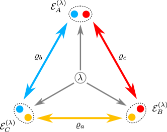
Figure 4: Triangle quantum network. Three sources $\varrho_{a}$, $\varrho_{b}$ and $\varrho_{c}$ distribute parties to three nodes, Alice, Bob and Charlie ($A$, $B$ and $C$). Alice, Bob and Charlie each end up with a bipartite system $X=X_{1}X_{2}$ on which they perform a local channel $\mathcal{E}_{X}^{(\lambda)}$ ($X=A,B,C$) depending on a classical random variable $\lambda$.

First, we note that in this definition, the state $\varrho_{ABC}$ does not depend on the classical variable $\lambda$. This is however, no restriction, as the dimensions of the source states are not bounded. If in Eq. (11) the $\varrho_{ABC}(\lambda)$ and hence the $\varrho_{a}(\lambda)$, $\varrho_{b}(\lambda)$, $\varrho_{c}(\lambda)$ depend on $\lambda$, one can just combine the set of all $\varrho_{a}(\lambda)$ to a single $\varrho_{a}$ etc. and redefine the maps $\mathcal{E}_{A}^{(\lambda)}$ etc. such that they act on the appropriate $\varrho_{a}(\lambda)$. This results in a form where $\varrho_{ABC}$ does not depend on $\lambda$ anymore, hence the state can be written as in Eq. (11). Note that this has already been observed in [27].

As mentioned in the main text, one may define network states also in a manner where the shared randomness is carried by the sources only. Indeed, if one adds an ancilla system to the source states, this may be used to identify the channel $\mathcal{E}_{X}$ to be applied. More explicitly, the source states may be redefined as $\varrho_{c}^{(\lambda)}\otimes|\lambda\rangle\langle\lambda|$ with orthogonal ancilla states $|\lambda\rangle$ being send to Bob (respectively to Charlie and Alice for sources $a$ and $b$), such that Bob can, by measuring $|\lambda\rangle$, decide which channel to apply. This measurement can then be seen as a global channel $\mathcal{E}_{B}$ that does not depend on $\lambda$. From the linearity of the maps, one may also write general network states as $\varrho=\mathcal{E}_{A}\otimes\mathcal{E}_{B}\otimes\mathcal{E}_{C}\big{[}\sum_{\lambda}p_{\lambda}\varrho_{ABC}^{(\lambda)}\big{]}$ as an equivalent definition. For our purpose, the potential dependence of $\varrho_{ABC}$ on $\lambda$ has the following consequence: If we wish to compute for a symmetric $|\psi\rangle$ the maximum fidelity $\langle\psi|\varrho|\psi\rangle$ over all network states $\varrho$, then we may assume that $\varrho$ permutationally symmetric, too. This follows from the simple fact that we can, without decreasing the overlap, symmetrize the state $\varrho_{ABC},$ and the symmetrized state will still be preparable in the network.

Second, one may restrict the $\varrho_{ABC}=\varrho_{a}\otimes\varrho_{b}\otimes\varrho_{c}$ further. Indeed it is straightforward to see that $\varrho_{a}=|a\rangle\langle a|$, $\varrho_{b}=|b\rangle\langle b|$, and $\varrho_{c}=|c\rangle\langle c|$ can be chosen to be pure, as the channels $\mathcal{E}_{A}^{(\lambda)}$ etc. are linear.

Third, as the set of network preparable states is by definition convex, one may ask for its extremal points. Formally, these are of the form $\mathcal{E}_{A}^{(\lambda)}\otimes\mathcal{E}_{B}^{(\lambda)}\otimes\mathcal{E}_{C}^{(\lambda)}\big{[}|a\rangle\langle a|\otimes|b\rangle\langle b|\otimes|c\rangle\langle c|\big{]},$ but can these further be characterized? Clearly, pure biseparable three-particle states, such as $|\psi\rangle=|\phi\rangle_{AB}\otimes|\eta\rangle_{C}$ are extremal points. There are however, also mixed states as extremal points, which can be seen as follows: It was shown in Ref. [26] that pure three-qubit states which are genuine multiparticle entangled (that is, not biseparable) cannot be prepared in the triangle network. On the other hand, in Ref. [27] it was shown that there are network states having a GHZ fidelity of 0.5170, which implies that they are genuine multiparticle entangled [41]. So, the set defined in Eq. (11) must have some extremal points, which are genuine multiparticle entangled mixed states.

After this prelude, let us explain the inflation technique [32, 17], which has already proven to be useful for the characterization of quantum networks [27]. We introduce it for triangle networks as for arbitrary networks it is a direct generalization.

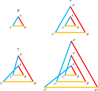
Figure 5: Triangle network and three of its inflations. The first figure represents the triangle network Supplementary Fig. 4, with global state $\varrho$. Using the same source states (represented by lines of same colour) and same local channels, one can build the so-called inflated state $\tau$, which is biseparable. The state $\gamma$ is build similarly, but with a different rewirering, leading to an inflated state that is in general not separable and different from $\tau$. One may also go to higher order inflations, e.g. with three copies and some rewireing, as depicted here. This procedure implies several equalities between the marginals of the original state and its inflations.

We start with constructing two inflations of the triangle network. Consider two networks with six vertices and six edges as in Supplementary Fig. 5. Identical sources are distributed along the lines of same colour, thus two copies of each source are needed per network. In other words, the source $\varrho_{b}$ is distributed between $AC$ and $A^{\prime}C^{\prime}$ to generated $\tau$, and between $AC^{\prime}$ and $A^{\prime}C$ for $\gamma$ (analogously for $\varrho_{a}$ and $\varrho_{c}$, following Supplementary Fig. 5). Then, the channels are performed according to the random parameter $\lambda$. Both on primed and non-primed $A$ nodes, the same channel $\mathcal{E}_{A}^{(\lambda)}$ is applied and similarly for $B$ and $C$. This leaves us with two network states, $\tau$ and $\gamma$. Those operators are physical states, i.e. they have a unit trace and are positive semi-definite. Formally, they can be written as

$$\tau= \sum_{\lambda}p_{\lambda}\Big{(}\mathcal{E}_{A}^{(\lambda)}\otimes\mathcal{E}_{B}^{(\lambda)}\otimes\mathcal{E}_{C}^{(\lambda)}\big{[}\varrho_{ABC}\big{]}\Big{)}\otimes\Big{(}\mathcal{E}_{A^{\prime}}^{(\lambda)}\otimes\mathcal{E}_{B^{\prime}}^{(\lambda)}\otimes\mathcal{E}_{C^{\prime}}^{(\lambda)}\big{[}\varrho_{A^{\prime}B^{\prime}C^{\prime}}\big{]}\Big{)}$$ (12)

and

$$\gamma= \sum_{\lambda}p_{\lambda}\mathcal{E}_{A}^{(\lambda)}\otimes\mathcal{E}_{B}^{(\lambda)}\otimes\mathcal{E}_{C}^{(\lambda)}\otimes\mathcal{E}_{A^{\prime}}^{(\lambda)}\otimes\mathcal{E}_{B^{\prime}}^{(\lambda)}\otimes\mathcal{E}_{C^{\prime}}^{(\lambda)}\big{[}\varrho_{ABCA^{\prime}B^{\prime}C^{\prime}}\big{]},$$ (13)

where $\varrho_{ABCA^{\prime}B^{\prime}C^{\prime}}=\varrho_{c}\otimes\varrho_{b}\otimes\varrho_{a}\otimes\varrho_{c}\otimes\varrho_{b}\otimes\varrho_{a}$, with the ordering of parties being different on both sides. Here, one needs to carefully pay attention to which channel acts on which party (this is depicted in Supplementary Fig. 5). Clearly, given only the knowledge of $\varrho$, the precise form of $\tau$ and $\gamma$ is not known. Still, due to the way they are constructed some of their marginals have to be equal, namely

$$\tau_{ABC} =\tau_{A^{\prime}B^{\prime}C^{\prime}}=\varrho,$$ (14)

$$\gamma_{ABC} =\gamma_{A^{\prime}B^{\prime}C^{\prime}},$$ (15)

$${\rm{Tr}}_{XX^{\prime}}(\tau) ={\rm{Tr}}_{XX^{\prime}}(\gamma)\quad{\rm for}\quad X=A,B,C.$$ (16)

Furthermore, from Eq. (12) it is clear that $\tau$ is separable wrt the partition $ABC|A^{\prime}B^{\prime}C^{\prime}$ and we note that $\tau$ and $\gamma$ are permutationally symmetric under the exchange of non primed and primed vertices. Therefore, if, for some given state $\varrho$, it is not possible to find states $\tau$ and $\gamma$ that satisfy those conditions, then $\varrho$ cannot be generated in the considered network.

An interesting point is that the question for the existence of $\tau$ and $\gamma$ with the desired properties can be directly formulated as a semidefinite program (SDP). This can be used to prove that such inflations do not exist, and the corresponding dual program can deliver an witness-like construction that can be used to exclude preparability of a state in the network. Still, these approaches are memory intensive. For instance, as the authors of Ref. [27] acknowledge, it is difficult to derive tests for tripartite qutrit states in a normal computer.

Finally, let us note that other triangle inflations may be considered, for instance inflations with $3n$ nodes ($n=3,4,\dots$) or simply wired differently than $\tau$ and $\gamma$. As mentioned previously, this technique can also be used for more complicated networks.

III Supplementary Note 2: Fidelity estimate for the GHZ state

Let us compute a bound on the fidelity of triangle network states to the GHZ state, i.e. compute $F=\max\langle GHZ|\varrho|GHZ\rangle$, where the maximum is taken over all states as in Eq. (11). For this maximization is it sufficient to consider the extremal states, which are of the type $\varrho_{ITN}=\mathcal{E}_{A}\otimes\mathcal{E}_{B}\otimes\mathcal{E}_{C}\big{[}\varrho_{ABC}\big{]}$, here $ITN$ stands for the independent triangle network, that is the triangle network without shared randomness.

Therefore, one may use techniques based on covariance matrices [29, 28], which are designed for the ITN. The covariance matrix (CM) $\Gamma$ of some random variables $x_{1},\dots,x_{N}$ is the matrix with elements $\Gamma_{ij}=\mathrm{cov}(x_{i},x_{j})=\left\langle x_{i}x_{j}\right\rangle-\left\langle x_{i}\right\rangle\left\langle x_{j}\right\rangle$, $i=1,\dots,N$.

We can now explain the general idea of the technique in Ref. [29]: If one computes the CM of the outcomes of $Z$-measurements on each qubit of an ITN state, then this matrix has a certain block structure. Checking this block structure can be done by checking the positivity of the comparison matrix $M(\Gamma)$. The comparison matrix obtained by flipping the signs of the off-diagonal elements of $\Gamma$. The condition then reads: For any quantum state in the ITN the comparison matrix of the CM is positive semi-definite. Hence, a negative eigenvalue in the comparison matrix excludes a state of being preparable in the ITN.

Now, if we apply that to states $\varrho(F)=F|GHZ\rangle\langle GHZ|+(1-F)\tilde{\varrho}$ with a fidelity $F$ to the GHZ state, the comparison matrix of the CM reads

$$M(\Gamma)=\begin{bmatrix}1-a^{2}(1-F)^{2}&-\left(F+d(1-F)-ab(1-F)^{2}\right)&-\left(F+e(1-F)-ac(1-F)^{2}\right)\\ -\left(F+d(1-F)-ab(1-F)^{2}\right)&1-b^{2}(1-F)^{2}&-\left(F+f(1-F)-bc(1-F)^{2}\right)\\ -\left(F+e(1-F)-ac(1-F)^{2}\right)&-\left(F+f(1-F)-bc(1-F)^{2}\right)&1-c^{2}(1-F)^{2}\\ \end{bmatrix},$$ (17)

where $a=\left\langle Z11\right\rangle_{\tilde{\varrho}}$, $b=\left\langle 1Z1\right\rangle_{\tilde{\varrho}}$, $c=\left\langle 11Z\right\rangle_{\tilde{\varrho}}$, $d=\left\langle ZZ1\right\rangle_{\tilde{\varrho}}$, $e=\left\langle Z1Z\right\rangle_{\tilde{\varrho}}$ and $f=\left\langle 1ZZ\right\rangle_{\tilde{\varrho}}$. From the last paragraph, we have that this matrix is positive semi-definite for ITN states, thus $\langle\phi|M(\Gamma)|\phi\rangle\geq 0$, for all vectors $|\phi\rangle$, and in particular for $|\phi\rangle=(1,1,1)/{\sqrt{3}}$. We notice that $\langle\phi|M(\Gamma)|\phi\rangle$ is upper bounded by $4-6F+F^{2}$ and therefore, $0\leq\langle\phi|M(\Gamma)|\phi\rangle\leq 4-6F+F^{2}$ holds for ITN states and we are able to exclude all states $\varrho(F)$ with $F>3-\sqrt{5}\simeq 0.7639$ form the triangle network scenario.

By making use of additional constraints or other criteria, we can obtain tighter bound. For any given three compatible dichotomic measurements $M_{1},M_{2},M_{3}$, we have [27]

$$p(M_{1}=M_{2})\geq p(M_{1}=M_{3})+p(M_{2}=M_{3})-1.$$ (18)

This implies

$$\left\langle M_{1}M_{2}\right\rangle\geq\left\langle M_{1}M_{3}\right\rangle+\left\langle M_{2}M_{3}\right\rangle-1.$$ (19)

By substituting $M_{i}$ with $-M_{i}$, we obtain

$$\left\langle M_{1}M_{2}\right\rangle\geq|\left\langle M_{1}M_{3}\right\rangle+\left\langle M_{2}M_{3}\right\rangle|-1,$$ (20)

$$\left\langle M_{1}M_{2}\right\rangle\leq 1-|\left\langle M_{1}M_{3}\right\rangle-\left\langle M_{2}M_{3}\right\rangle|.$$ (21)

In our case, we have

$$d\geq|a+b|-1,\quad e\geq|a+c|-1,\quad f\geq|b+c|-1.$$ (22)

With this extra constraint, $0\leq\langle\phi|M(\Gamma)|\phi\rangle\leq 9-12F$ holds for ITN states and we are able to exclude all states $\varrho(F)$ with $F>3/4=0.75$ form the triangle network scenario.

Another criterion for ITN states [23] states that

$$(1+|E_{A}|+|E_{B}|+E_{AB})^{2}$$

$$+ (1+|E_{A}|+|E_{C}|+E_{AC})^{2}$$

$$+ (1+|E_{B}|+|E_{C}|+E_{BC})^{2}$$

$$\leq 6(1+|E_{A}|)(1+|E_{B}|)(1+|E_{C}|),$$ (23)

where

$$E_{A}=\left\langle Z11\right\rangle_{\varrho},\ E_{B}=\left\langle 1Z1\right\rangle_{\varrho},\ E_{C}=\left\langle 11Z\right\rangle_{\varrho},$$ (24)

$$E_{AB}=\left\langle ZZ1\right\rangle_{\varrho},\ E_{AC}=\left\langle Z1Z\right\rangle_{\varrho},\ E_{BC}=\left\langle 1ZZ\right\rangle_{\varrho}.$$ (25)

As it turns out, if Eq. (III) together with Eq. (22) has a feasible solution of $a,b,c,d,e,f\in[-1,1]$, then $F$ should be no more than $1/\sqrt{2}\simeq 0.7071$. Hence, we can exclude all states $\varrho(F)$ with $F>1/\sqrt{2}\simeq 0.7071$ form the triangle network scenario.

In particular, if we know $E_{A}=E_{B}=E_{C}=0$, i.e., $a=b=c=0$, Eq. (III) reduces to

$$6\geq \ (1+F+d(1-F))^{2}+(1+F+e(1-F))^{2}$$

$$+(1+F+f(1-F))^{2}$$

$$\geq \ 3(1+F-(1-F))^{2}$$

$$= \ 12F^{2},$$ (26)

which implies $F\leq 1/\sqrt{2}$. The bound $1/\sqrt{2}\simeq 0.7071$ is slightly worse, but close to the one $0.6803$ obtained in Ref. [27] based on advanced numerical computations.

IV Supplementary Note 3: Graph and cluster states

In this Supplementary Note we present our results on graph states and cluster states. It is structured as follows: We first recall the basic facts about graph and cluster states. Then, we prove the estimate on the fidelity with cluster states for states in the square network (see the main text). Finally, we present the proof and discussion of Observation 1.

IV.1 Graph states and the stabilizer formalism

Graph states [55, 46] are quantum states defined through a graph $G=(V,E)$, i.e. through a set $V$ of $N$ vertices and a set $E$ containing edges that connect the vertices. The vertices represent the physical systems, qubits. One way of describing these states is through the stabilizer formalism. For that, as introduced in the main text, one first needs to introduce the generator operators $g_{i}$ of graph states: a graph state $|G\rangle$ is the unique common $+1$-eigenstate of the set of operators $\{g_{i}\}$,

$$g_{i}=X_{i}\prod_{j\in\mathcal{N}_{i}}Z_{j},$$ (27)

where $\mathcal{N}_{i}$ is the neighbourhood of the qubit $i$, i.e. the set of all qubits $j\in V$ connected to the qubit $i\in G$. The state $|G\rangle$ can also be described through its stabilizer, which is the set $\mathcal{S}=\{S_{1},\dots,S_{2^{N}}\}=\{\prod_{i=1}^{N}g_{i}^{x_{i}}:\{x_{1},\dots,x_{N}\}\in\{0,1\}^{N}\}$. This means that $\mathcal{S}$ contains all possible products of the generators $g_{i}$, hence $S_{i}|G\rangle=|G\rangle$. We note that $\mathds{1}\in\mathcal{S}$. The projector onto the state $|G\rangle$ reads

$$|G\rangle\langle G|=\frac{1}{2^{N}}\sum_{i=1}^{2^{N}}S_{i}.$$ (28)

Defined like that, graph states are a subset of the more general stabilizer states [45, 47, 46]. First, one has to consider an abelian subgroup $\mathcal{S}$ of the Pauli group $\mathcal{P}_{N}$ on $N$ qubits that does not contain the operator $-\mathds{1}$. To that set corresponds a vector space $V_{\mathcal{S}}$ that is said to be stabilized by $\mathcal{S}$, i.e. every element of this vector space is stable under the action of any element of $\mathcal{S}$. We call stabilizers that lead only to one state full-rank stabilizers, i.e. there is a unique common eigenstate with eigenvalue $+1$. That state is completely determined by a subset of $N$ elements of $\mathcal{S}$. As an example, one may consider the GHZ state, as explained in the main text. Indeed, it is the unique common eigenstate of $XXX$, $1ZZ$ and $ZZ1$. One can show that any stabilizer state is, after a suitable local unitary transformation, equivalent to a graph state.

More precisely, the local unitary transformations that map any stabilizer state to a graph state belong to the so-called local Clifford group $\mathcal{C}_{1}$. The local Clifford group is defined as the normalizer of the single-qubit Pauli group, i.e. $U\mathcal{P}_{1}U^{\dagger}=\mathcal{P}_{1}$ for all $U\in\mathcal{C}_{1}$. By construction, the stabilizer formalism is preserved under the action of the local Clifford group, and hence, an interesting question is under which conditions two graph states (or two stabilizer states) are equivalent under local Cliffords. For graph states this question has a simple solution in terms of graphical operations that determine their equivalence. Namely, two graph states are equivalent under the action of the local Clifford group if and only if their corresponding graphs are equivalent under a sequence of local complementations [54]. For a given graph $G$ and vertex $i\in V$ the local complement $G^{\prime}$ of $G$ at the vertex $i$ is constructed in two steps. First, we have to determine the neighborhood $N(i)\subset V$ of the vertex $i$ and then the induced subgraph is inverted, i.e. considering all possible edges in the neighborhood any pre-existing edge is removed and any non-existing edge is added. E.g. having a graph $V=\{1,2,3\}$ and $E=\{(1,2),(2,3),(3,1)\}$, a local complementation on vertex $1$ results in the graph with edges $E=\{(1,2),(3,1)\}$.

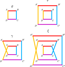
Figure 6: Square network and three of its inflations. Similar to the triangle network of Supplementary Fig. 5, the states $\tau$ and $\gamma$ are generated using two copies of the sources and channels used to generate $\varrho$, without and with rewireing respectively. Then, one goes to a high order inflation by using three copies of the sources and the local channels. By rewireing according to the figure, one gets the inflated state $\xi$. Due to the way network states are generated, several of the marginals of $\varrho$, $\tau$, $\gamma$ and $\xi$ are identical.

IV.2 Estimate for the cluster state fidelity

We aim at computing a bound on the fidelity of square network states to the four-qubit ring cluster state $|C_{4}\rangle$, i.e. $F=\mathrm{max}\langle Cl_{4}|\varrho|Cl_{4}\rangle$, were the maximum is taken over all square network states $\varrho$. The fidelity of a state $\varrho$ with the cluster state is given by $F=\frac{1}{16}\sum_{i=0}^{15}\left\langle S_{i}\right\rangle_{\varrho}$, where $\{S_{i}\}$ is the stabilizer of $|C_{4}\rangle$, consisting of $S_{0}=1111$ and further elements given in Supplementary Table 1.

Stabilizer elements
$S_{1}=XZ1Z$	$S_{5}=YYZZ$	$S_{9}=X1X1$	$S_{11}=-YXY1$	$S_{15}=XXXX$
$S_{2}=ZXZ1$	$S_{6}=YZZY$	$S_{10}=1X1X$	$S_{12}=-1YXY$
$S_{3}=1ZXZ$	$S_{7}=ZYYZ$		$S_{13}=-Y1YX$
$S_{4}=Z1ZX$	$S_{8}=ZZYY$		$S_{14}=-XY1Y$
$\left\langle\cdot\right\rangle_{\varrho}=\Theta$	$\left\langle\cdot\right\rangle_{\varrho}=\Lambda$	$\left\langle\cdot\right\rangle_{\varrho}=\Xi$	$\left\langle\cdot\right\rangle_{\varrho}=-\Sigma$	$\left\langle\cdot\right\rangle_{\varrho}=\Omega$

Table 1: Elements of the stabilizer of the four-qubit cluster states. The qubit indices $A,B,C,D$ are suppressed here. See the text for further details.

The symmetry of $|C_{4}\rangle$ implies that one can assume the network state $\varrho$ that maximizes the fidelity to admit the same expectation value on operators from the same column, as denoted in the last row of Supplementary Table 1.

As explained in the main text, the general idea is to notice that some stabilizers of $|C_{4}\rangle$ anticommute in the appropriate inflation, and then use the fact that anticommuting operators cannot all have large expectation values for a given state. In the $\tau$-inflation of the square network (see Supplementary Fig. 6), the observable $X_{B}X_{D^{\prime}}$ and $Y_{A}Y_{B}Z_{C}Z_{D}$ anticommute, and since $\tau_{BD^{\prime}}=\varrho_{BD}$ and $\tau_{ABCD}=\varrho_{ABCD}$ one has

$$\Xi^{2}+\Lambda^{2}\leq 1.$$ (29)

Secondly, we have Eq. (9) of the main text that we reformulate as

$$\Xi^{2}+\Theta^{2}+\Sigma^{2}\leq 1.$$ (30)

At last, we consider the observables $X_{A}X_{B}X_{C}X_{D}$ and $Z_{A}X_{B}Z_{A^{\prime}}X_{D^{\prime}}$ in the inflation $\tau$. However, the latter is not a stabilizer of the four-qubit ring cluster state, but we have $\left\langle Z_{A}X_{B}Z_{A^{\prime}}X_{D^{\prime}}\right\rangle_{\tau}=\left\langle Z_{A}X_{B}Z_{A^{\prime}}X_{D}\right\rangle_{\gamma}$. Then, using the fact that for commuting dichotomic measurements, $\left\langle M_{1}M_{2}\right\rangle\geq\left\langle M_{1}M_{3}\right\rangle+\left\langle M_{2}M_{3}\right\rangle-1$ [27], one gets $\left\langle Z_{A}X_{B}X_{D}Z_{A^{\prime}}\right\rangle_{\gamma}\geq\left\langle Z_{A}X_{B}Z_{C}\right\rangle_{\gamma}+\left\langle Z_{C}X_{D}Z_{A^{\prime}}\right\rangle_{\gamma}-1$. Since $X_{A}X_{B}X_{C}X_{D}$ and $Z_{A}X_{B}Z_{A^{\prime}}X_{D^{\prime}}$ are anticommuting, from constraints on the marginals, one finally gets

$$\begin{split}2\Theta-1\leq\sqrt{1-\Lambda^{2}}.\end{split}$$ (31)

Analogously,

$$2\Sigma-1\leq\sqrt{1-\Lambda^{2}},$$ (32)

$$2\Theta-1\leq\sqrt{1-\Omega^{2}},$$ (33)

$$2\Sigma-1\leq\sqrt{1-\Omega^{2}}.$$ (34)

By exploiting all these inequalities as constraints on the maximization of the fidelity, we finally get

$$\begin{split}F&=\frac{1}{16}\big{(}1+4\Theta+4\Lambda+2\Xi-4\Sigma+\Omega\big{)}\\ &\leq 0.737684,\end{split}$$ (35)

hence all states with a larger fidelity to the four-qubit ring cluster state cannot be prepared in a square network.

IV.3 Proof of Observation 1

Here we provide a detailed proof of Observation 1. To do so, we first need to prove the following theorem.

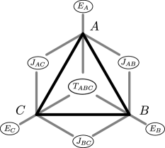
Figure 7: Illustration of the conditions in Theorem 3. We consider a triangle in the graph of a graph state. The vertices $A,B,C$ share some neighbourhoods, which are indicated by black ellipses. Note that the graph may contain further vertices, also the vertices in different neighbourhoods may be connected. See the text for further details.

Theorem 3.

Let $G(V,E)$ be a graph as in Supplementary Fig. 7 with three mutually connected vertices $A$, $B$ and $C$ and let

$$T_{ABC}=\mathcal{N}_{A}\cap\mathcal{N}_{B}\cap\mathcal{N}_{C},$$ (36)

$$J_{AB}=(\mathcal{N}_{A}\cap\mathcal{N}_{B})\setminus T_{ABC},$$ (37)

$$E_{A}=\mathcal{N}_{A}\setminus(\mathcal{N}_{B}\cup\mathcal{N}_{C}),$$ (38)

etc., where $\mathcal{N}_{X}$ is the neighborhood of $X$ ($X=A,B,C$). Then the graph state $|G\rangle$ cannot originate from any network with only bipartite sources, if one of the following conditions is satisfied:

1. $J_{XY}=J_{XZ}=\emptyset$, where $X,Y,Z$ is a permutation of $A,B,C$;

2. $E_{X}=E_{Y}=\emptyset$, where $X\neq Y\in\{A,B,C\}$ ;

3. $E_{X}=J_{XY}=\emptyset$, where $X\neq Y\in\{A,B,C\}$.

Proof.

We only need to show that the graph state $|G\rangle$ cannot be generated in the network with the complete graph $K$ as shown in Supplementary Fig. 8, where the number of vertices is the same than in $G$.

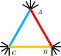
Figure 8: The bipartite network with complete graph $K$. This is the network that should generate the graph state from Supplementary Fig. 7. Note that here the bipartite links of the network are shown, and not the edges of the graph of the graph state.

We start our discussion with the inflation $\gamma$ as in Supplementary Fig. 9.

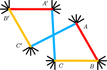
Figure 9: The network for the inflation $\gamma$. This is a two-copy inflation, where only the links between $AC$ and $A^{\prime}C^{\prime}$ are rewired.

Let us denote

$$g_{A}=X_{A}Z_{\mathcal{N}_{A}},\quad g_{B}=X_{B}Z_{\mathcal{N}_{B}},\quad g_{C}=X_{C}Z_{\mathcal{N}_{C}},$$ (39)

where $\mathcal{N}_{A}$ is the neighborhood of the vertex $A$ in the graph $G$. Then

$$g_{A}g_{B}=Y_{A}Y_{B}Z_{R_{AB}},$$ (40)

$$g_{A}g_{C}=Y_{A}Y_{C}Z_{R_{AC}},$$ (41)

$$g_{B}g_{C}=Y_{B}Y_{C}Z_{R_{BC}},$$ (42)

where $R_{AB}={E_{A}\cup E_{B}\cup J_{AC}\cup J_{BC}}$, and analoguously for $R_{AC}$ and $R_{BC}$. Since $g_{A}g_{C}=(g_{A}g_{B})(g_{B}g_{C})$, we can apply the usual argument from the GHZ state to conclude that

$$\left\langle Y_{A}Y_{C}Z_{R_{AC}}\right\rangle_{\gamma}\geq\left\langle Y_{A}Y_{B}Z_{R_{AB}}\right\rangle_{\gamma}+\left\langle Y_{B}Y_{C}Z_{R_{BC}}\right\rangle_{\gamma}-1.$$ (43)

By comparing the marginals of the states $\gamma$ and $\varrho$, we have

$$\left\langle Y_{A}Y_{B}Z_{R_{AB}}\right\rangle_{\gamma}=\left\langle Y_{A}Y_{B}Z_{R_{AB}}\right\rangle_{\varrho},$$ (44)

$$\left\langle Y_{B}Y_{C}Z_{R_{BC}}\right\rangle_{\gamma}=\left\langle Y_{B}Y_{C}Z_{R_{BC}}\right\rangle_{\varrho},$$ (45)

since $A,C\not\in R_{AB}\cup R_{BC}$. In the following, we will also use the notation

$$\mathcal{R}=R_{AC}=E_{A}\cup E_{C}\cup J_{AB}\cup J_{BC}$$ (46)

in order to avoid a plethora of indices.

Then, we consider the inflation $\eta$ shown in Supplementary Fig. 10. This is constructed as follows. First, one has two disconnected complete graphs, $K$ and $K^{\prime}$. Then, one takes the subset $\mathcal{R}$ as a subgraph of $K$ and rewires all connections from vertices in $\mathcal{R}$ to $A$ to $A^{\prime}$. Similarly, one takes the subset $\mathcal{R^{\prime}}$ as a subgraph of $K^{\prime}$ and rewires all connections from vertices in $\mathcal{R^{\prime}}$ to $A^{\prime}$ to $A$.

By comparing the marginals of $\gamma$ and $\eta$, this time we have

$$\left\langle Y_{A}Y_{C}Z_{\mathcal{R}}\right\rangle_{\gamma}=\left\langle Y_{A^{\prime}}Y_{C}Z_{\mathcal{R}}\right\rangle_{\eta}.$$ (47)

With this reasoning, we have established that the correlation $\left\langle Y_{A^{\prime}}Y_{C}Z_{\mathcal{R}}\right\rangle_{\eta}$ is large in $\eta$, if the original state $\varrho$ is close to the graph state. Now we have to identify another anticommuting observables in $\eta$ with large expectation value in order to arrive at a contradiction.

A natural first candidate is the stabilizing operator

$${g}_{B}=X_{B}Z_{A}Z_{C}Z_{\mathfrak{R}}.$$ (48)

with $\mathfrak{R}=E_{B}\cup J_{AB}\cup J_{BC}\cup T_{ABC}$ of the graph state. This, however, cannot always be identified with some observable in the inflation $\eta$. Still, if

$$\mathcal{R}\cap\mathfrak{R}=\emptyset\Leftrightarrow J_{AB}=J_{BC}=\emptyset$$ (49)

the observable ${g}_{B}$ is not affected by the rewiring in $\eta$, we have $\left\langle{g}_{B}\right\rangle_{\varrho}=\left\langle{g}_{B}\right\rangle_{\eta}$. Moreover, in $\eta$ the observables $g_{B}$ and $Y_{A}^{\prime}Y_{C}Z_{\mathcal{R}}$ anticommute. So, in this case we have

$$\left\langle Y_{A}Y_{C}Z_{\mathcal{R}}\right\rangle_{\gamma}^{2}+\left\langle{g}_{B}\right\rangle_{\eta}^{2}\leq 1.$$ (50)

and for the original $\varrho$ we arrive at the condition (assuming $\left\langle Y_{A}Y_{B}Z_{R_{AB}}\right\rangle_{\varrho}+\left\langle Y_{B}Y_{C}Z_{R_{BC}}\right\rangle_{\varrho}-1\geq 0$, as in Eq. (6) in the main text)

$$(\left\langle Y_{A}Y_{B}Z_{R_{AB}}\right\rangle_{\varrho}+\left\langle Y_{B}Y_{C}Z_{R_{BC}}\right\rangle_{\varrho}-1)^{2}+\left\langle{g}_{B}\right\rangle_{\varrho}^{2}\leq 1$$ (51)

for states that can be prepared in the network.

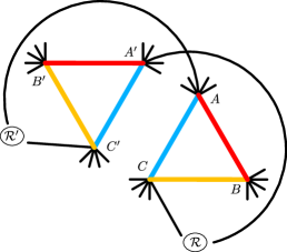
Figure 10: The network for the inflation $\eta$. This is constructed as follows. First, one has two disconnected complete graphs, $K$ and $K^{\prime}$. Then, one takes the subset $\mathcal{R}$ as a subgraph of $K$ and rewires all connections from vertices in $\mathcal{R}$ to $A$ to $A^{\prime}$. Similarly, one takes the subset $\mathcal{R^{\prime}}$ as a subgraph of $K^{\prime}$ and rewires all connections from vertices in $\mathcal{R^{\prime}}$ to $A^{\prime}$ to $A$.

Furthermore, in the case that $E_{A}=E_{C}=\emptyset$ and by making use of the operator

$${g}_{A}{g}_{B}{g}_{C}=X_{A}X_{B}X_{C}Z_{E_{B}\cup T_{ABC}},$$ (52)

we arrive at a similar condition on $\varrho$ that is also violated by the graph state $|G\rangle$.

Finally, if $E_{A}=J_{AB}=\emptyset$, one can make use of the operator

$${g}_{A}=X_{A}Z_{B}Z_{C}Z_{J_{AC}\cup T_{ABC}},$$ (53)

in order to arrive at a condition on $\varrho$ that is not satisfied by the graph state $|G\rangle$.

By permuting $A,B,C$ in the above argument, we finish our proof. ∎

In the following, we identify some basic situations where the Theorem 3 can be applied. First, we show that the conditions of Theorem 3 are met, if there is one vertex with a small degree.

Corollary 4.

Let $G$ be connected graph with no less than three vertices. If its minimal degree is no more than three, the graph state $|G\rangle$ cannot be generated by any network with bipartite sources.

Proof.

The proof will be done successively for minimal degree one, two and three.

Let $v$ be a vertex whose degree is one and let $w$ be the vertex connected to $v$. Since $G$ is a connected graph with no less than three vertices,

$$\mathcal{N}_{w}\setminus\{v\}\neq\emptyset,$$ (54)

where $\mathcal{N}_{w}$ is the neighbourhood of $w$. If we apply local complementation on the vertex $w$, we obtain a new graph $G^{\prime}$, where

$$u\sim v,\quad\forall u\in\mathcal{N}_{w}\setminus\{v\},$$ (55)

where $u\sim v$ means that the vertices $u,v$ are connected.

By setting

$$B=w,\quad A=v,\quad C=u_{0},$$ (56)

where $u_{0}$ is an arbitrary vertex in $\mathcal{N}_{w}\setminus\{v\}$, we see that

$$\begin{split}&\mathcal{N}_{B}\setminus\{A,C\}=T_{ABC}\cup J_{AB},\\ &A\sim B,\quad A\sim C,\quad B\sim C.\end{split}$$ (57)

Hence, $E_{B}=J_{BC}=\emptyset$, which implies $|G^{\prime}\rangle$ cannot be from any network with only bipartite sources. Since $|G\rangle$ is equivalent to $|G^{\prime}\rangle$ up to a local unitary transformation, we come to the same conclusion for $|G\rangle$.

Now, let us consider graphs with minimal degree equal to two, and let $v$ be a vertex with degree two, and $w$ and $u$ be the two vertices connected to $v$. If $w\not\sim u$, we can apply a local complementation on $v$ to connect them. Hence, we can assume $w\sim u$ without loss of generality. By setting

$$A=w,\quad B=v,\quad C=u,$$ (58)

we have

$$E_{B}=J_{AB}=J_{BC}=T_{ABC}=\emptyset,$$ (59)

which leads to the desired conclusion.

Lastly, let $v$ be a vertex with degree three and let $w$, $u$ and $t$ be the three vertices connected to $v$. Since we can apply local complementation on $v$, without loss of generality, we can assume that there are at least two edges among $w$, $u$ and $t$, more specifically, $w\sim u$ and $w\sim t$. Let us take

$$A=w,\quad B=v,\quad C=u,$$ (60)

hence we see that

$$E_{B}=\emptyset,\quad J_{AB}=\emptyset\quad\text{or}\quad J_{BC}=\emptyset.$$ (61)

This implies that the graph state $|G\rangle$ with a vertex of degree three cannot be from any network with only bipartite sources. ∎

Under certain conditions, we can also exclude a network structure for graphs with minimal degree four:

Corollary 5.

Let $G$ be a graph that has a vertex $v$ of degree four. If the induced subgraph on the neighborhood $\mathcal{N}_{v}$ is not a line graph, then $|G\rangle$ cannot be generated in any network with bipartite sources.

Proof.

As shown in Supplementary Fig. 11, there are six inequivalent graphs with four vertices up to permutation and complementation.

Figure 11: The six inequivalent graphs with four vertices up to permutations and complementation.

In case (a), we can set $B=v,A=u_{1},C=u_{2}$, then

$$T_{ABC}=\{u_{3},u_{4}\},\quad E_{B}=J_{AB}=J_{BC}=\emptyset.$$ (62)

In case (b) and (c), we can set $B=v,A=u_{3},C=u_{4}$, then

$$E_{B}=\{u_{1},u_{2}\},\quad J_{AB}=J_{BC}=T_{ABC}=\emptyset.$$ (63)

In case (d) and (e), we can set $B=v,A=u_{1},C=u_{3}$, then

$$E_{B}=\{u_{2}\},\quad T_{ABC}=\{u_{4}\},\quad J_{AB}=J_{BC}=\emptyset.$$ (64)

In all the above cases, Theorem 3 implies that the graph state $|G\rangle$ cannot be from any network with only bipartite sources. In case (f), the neighbourhood $\mathcal{N}_{v}$ of $v$ is a line graph whose complementation is also a line graph. ∎

Having established these results, we can discuss graphs with a small number of vertices. Here. previous works have established a classification of all small graphs with respect to equivalence classes under local complementation. In detail, this classification has been achieved for up to seven vertices in Ref. [55], for eight vertices in Ref. [56] and for nine to twelve vertices in Ref. [58]. These required numerical techniques are advanced, as, for instance, for twelve qubits already $1~{}274~{}068$ different equivalence classes under local complementation exist. We can use this classification now, and apply our result on it to obtain:

Theorem 6.

No graph state with up to twelve vertices can originate from a network with only bipartite sources.

Proof.

Using the tables in Ref. [58] one can directly check that except the graph $G_{d5}$ in Supplementary Fig. 12, all graphs with no more than twelve vertices, up to isomorphism and local complementation, satisfy at least one condition in Corollary 4 and 5.

For the graph $G_{d5}$, the minimal degree is no less than $5$ whatever local complementation is applied. However, if we set

$$B=v_{1},\quad A=v_{4},\quad C=v_{5},$$ (65)

then

$$E_{B}=\{v_{2},v_{3}\},\quad T_{ABC}=\{v_{6}\}.$$ (66)

Thus, $J_{AB}=J_{BC}=\emptyset$, which implies that the graph state $|G_{d5}\rangle$ cannot originate from a network with only bipartite sources.

All in all, no graph state with more than twelve vertices can originate from a network with only bipartite sources. ∎

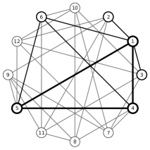
Figure 12: The graph $G_{d5}$ with twelve vertices, where the minimal degree is no less than five whatever local complementation is applied.

The statements in Observation 1 concerning the two- or three-dimensional cluster states follow directly from Corollary 5 (in the 2D case) or the application of a local complementation and Theorem 3.

IV.4 Networks with tripartite sources

Let us finally discuss two examples of networks with tripartite sources. First, one may expand the method used in the main text to exclude the GHZ state of the set of network states. Consider the fully connected four-partite graph state, which is locally equivalent to the four-partite GHZ state and let us show that it cannot have originated from the four partite network with four tripartite sources, illustrated in Supplementary Fig. 13. Consider the $\nu$- and $\tau$-inflations of that network, depicted in Supplementary Fig. 14. From $\left\langle Y_{i}Y_{k}\right\rangle_{\nu}\geq\left\langle Y_{i}Y_{j}\right\rangle_{\nu}+\left\langle Y_{j}Y_{k}\right\rangle_{\nu}-1$ and the marginal equalities, one gets $\left\langle Y_{A}Y_{A^{\prime}}\right\rangle_{\tau}\geq\left\langle Y_{A}Y_{B}\right\rangle_{\varrho}+\left\langle Y_{B}Y_{C}\right\rangle_{\varrho}+\left\langle Y_{C}Y_{D}\right\rangle_{\varrho}+\left\langle Y_{D}Y_{A}\right\rangle_{\varrho}-3$. Then, from an anticommuting relation in the $\tau$-inflation and marginal equalities, one gets $\left\langle Y_{A}Y_{A^{\prime}}\right\rangle_{\tau}^{2}+\left\langle X_{A}Z_{B}Z_{C}Z_{D}\right\rangle_{\varrho}^{2}\leq 1$. Combining those two equations, one gets that a fidelity higher than $0.923$ to the the fully connected graph state cannot be achieved by a four-partite network state.

Second, consider the graph state $|G\rangle$ whose graph is represented in Supplementary Fig. 15 (note that it is equivalent under local complementation to the fully connected graph state with the edge between $A$ and $D$ missing). Now, consider a six-partite network with six tripartite sources, connected as in Supplementary Fig. 16. One can show that the observables $X_{A}X_{D^{\prime\prime}}$, $Z_{A}X_{B}Z_{D}$ and $Y_{A}Y_{E^{\prime}}X_{D}$ anticommute in the $\xi$-inflation of the network (see Supplementary Fig. 17) and thus get to an inequality for any state $\varrho$ in the considered network, $\left\langle X_{A}X_{D}\right\rangle_{\varrho}^{2}+\left\langle Z_{A}X_{B}Z_{D}\right\rangle_{\varrho}^{2}+\left\langle Y_{A}Y_{E}X_{D}\right\rangle_{\varrho}^{2}\leq 1$, where all three observables are in the stabilizer of $|G\rangle$. Seven other inequalities of that type can be derived, and using them one gets that no state with a fidelity to $|G\rangle$ higher that $0.949$ can be prepared in the quantum network of Supplementary Fig. 16.

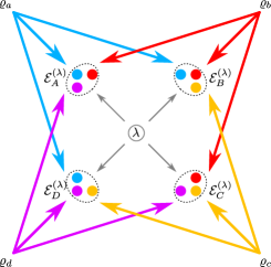
Figure 13: Square network with four tripartite sources.

Figure 14: The $\tau$- and $\nu$-inflations of the square network with tripartite sources.

Figure 15: A six-partite graph state $|G\rangle$.

Figure 16: Hexagon network with six tripartite sources.

Figure 17: The $\xi$-inflation of the hexagon network with tripartite sources.

From these two examples, we see that the anticommuting relation method also holds for networks with more then bipartite sources. However, it remains an open question whether it leads to general results similar to those of Observation 1.

V Supplementary Note 4: Permutationally symmetric states

Before proving our main results, let us give some definitions. As introduced in the main text, we define $N$-partite permutationally symmetric (bosonic) states as states that satisfy $\Pi^{+}_{ij}\varrho\Pi^{+}_{ij}=\varrho$ for all $i,j\in\{1,\dots,N\}$ with $2\Pi^{+}_{ij}=\mathds{1}+F_{ij}$ and $F_{ij}$ being the flip operator that exchanges parties $i$ and $j$. We can also introduce fermionic states that are antisymmetric for a pair of parties $\{ij\}$, i.e. $\Pi^{-}_{ij}\varrho\Pi^{-}_{ij}=\varrho$, with $2\Pi^{-}_{ij}=\mathds{1}-F_{ij}$. For our discussion we need several basic facts. We stress that the following Lemma 7 and 9 are well known [36, 48, 39], while Lemma 8 is a simple technical statement.

Lemma 7.

Let $\varrho=\sum_{k}p_{k}|\psi_{k}\rangle\langle\psi_{k}|$ be a multipartite state and let $\Pi$ be a projector such that $\Pi\varrho\Pi=\varrho$. Then $\Pi|\psi_{k}\rangle=|\psi_{k}\rangle$ for all $k$.

Proof.

One has

$$\begin{split}1={\rm{Tr}}(\varrho)=&{\rm{Tr}}(\Pi\varrho\Pi)\\ =&\sum_{k}p_{k}\langle\psi_{k}|\Pi|\psi_{k}\rangle.\end{split}$$ (67)

So $\langle\psi_{k}|\Pi|\psi_{k}\rangle=1$, and since $\Pi$ is a projector, $\Pi|\psi_{k}\rangle=|\psi_{k}\rangle$, for all $k$. ∎

This holds in particular for $\Pi=\Pi_{ij}^{\pm}$. As a second lemma, we have

Lemma 8.

If the reduced state on $AB$ of some state is symmetric or antisymmetric under the exchange of parties $A$ and $B$, then the global state also is.

Proof.

Let $\varrho=\sum_{k}p_{k}|\psi_{k}\rangle\langle\psi_{k}|$ be the state of some tripartite system $ABC$. Let us prove that if $F_{AB}\left({\rm{Tr}}_{C}(\varrho)\right)=\pm{\rm{Tr}}_{C}(\varrho)$, then $(F_{AB}\otimes\mathds{1})\varrho=\pm\varrho$. If one considers the Schmidt decomposition of $|\psi_{k}\rangle$ wrt the bipartition $AB|C$, one has

$$\varrho=\sum_{k}p_{k}\sum_{i,j}s_{k,i}s_{k,j}^{*}|\phi_{k,i}^{AB}\rangle\langle\phi_{k,j}^{AB}|\otimes|\chi_{k,i}^{C}\rangle\langle\chi_{k,j}^{C}|.$$ (68)

From that, $\varrho_{AB}=\sum_{k}p_{k}\sum_{i}|s_{k,i}|^{2}|\phi_{k,i}^{AB}\rangle\langle{\phi_{k,i}^{AB}}|$ and since it is a permutationally symmetric (respectively antisymmetric) state, from Lemma 7 all states in its decomposition also are and thus $(F_{AB}\otimes\mathds{1})\varrho=\pm\varrho$. ∎

We note that for both those lemma, the converse is trivial. Finally, we have:

Lemma 9.

(a) A $N$-partite symmetric state $\varrho_{s}$ is either genuinely $N$-partite entangled or fully separable. (b) A $N$-partite antisymmetric state is always $N$-partite entangled.

Proof.

Due to Lemma 7 we only need to consider pure states. Let $|\Psi\rangle$ be a $N$-partite (anti)symmetric state that is not $N$-partite entangled, hence it is separable for some bipartition. Without loss of generality, we assume that

$$|\Psi\rangle=|\varphi_{1,\dots,t}\rangle\otimes|\phi_{t+1,\dots,N}\rangle.$$ (69)

Thus, by tracing out the first $t$ parties, we have a pure state. The symmetry of $|\Psi\rangle$ implies that the reduced state is pure after tracing out any $t$ parties. This can only be true if $|\varphi_{1,\ldots,t}\rangle,|\phi_{t+1,\ldots,N}\rangle$ are fully separable.

Besides, denote $|ab\ldots c\rangle$ a normalized fully separable antisymmetric state, we have $|ab\ldots c\rangle=-|ba\ldots c\rangle$. This implies that $-1=\left\langle ab\ldots c|ba\ldots c\right\rangle=|\left\langle a|b\right\rangle|^{2}\geq 0$, hence we arrive at a contradiction. ∎

We note that the notions of entanglement used in this Lemma are the standard ones for non-symmetric states, as these are the relevant ones for the main text. In principle, for indistinguihable particles one may separate the ‘‘formal" entanglement due to the wave function symmetrization from the ‘‘physical" entanglement [36].

Now, let us prove the Observation 2 of the main text. For completeneness, we restate it here in the full formulation:

Observation 2’. Let $\varrho$ be a permutationally symmetric multiparticle state. Then, $\varrho$ can be generated in a quantum network with $N-1$-partite sources if and only if it is fully separable. If $\varrho$ be a permutationally antisymmetric, then it cannot be generated in a network.

Proof.

Let $\varrho$ be a $N$-partite permutationally (anti)symmetric state. Let us assume that it can be generated in a network of $N$ nodes with some at most $(N-1)$-partite sources. Note that any state that can be generated in a network of $N$ nodes with no $N$-partite sources, can also be generated in a network of $N$ nodes with $N$ different $(N-1)$-partite sources. Let us denote by $\varsigma_{i}$ the source used to generate $\varrho$ that distributes parties to all nodes except the $i$th one.

If we assume that $\varrho$ is a network state, then the inflation $\eta$ build the following way is a physical state: Consider a network of $2N$ nodes $\{A_{i},A^{\prime}_{i}:i=1,\dots,N\}$ and $2N$ sources $\{\zeta_{k},\zeta^{\prime}_{k}:k=1,\dots,N\}$ that distribute parties to

$$\zeta_{k}:A_{1}\ldots A_{k-1}A^{\prime}_{k+1}\ldots A^{\prime}_{N},$$ (70)

$$\zeta^{\prime}_{k}:A^{\prime}_{1}\ldots A^{\prime}_{k-1}A_{k+1}\ldots A_{N},$$ (71)

where $\zeta_{k}=\zeta^{\prime}_{k}=\varsigma_{k}$ for all $k$. The state $\eta$ is the network state build with these sources and the same channels on the nodes than $\varrho$ (with some shared randomness). From the inflation technique, we know that for the reduced states

$$\eta_{A_{i}A_{i+1}}=\eta_{A^{\prime}_{i}A^{\prime}_{i+1}}=\varrho_{A_{i}A_{i+1}},\quad\forall i\leq N-1,$$ (72)

$$\eta_{A_{1}A^{\prime}_{N}}=\eta_{A^{\prime}_{1}A_{N}}=\varrho_{A_{1}A_{N}}.$$ (73)

Since the state $\varrho$ is fully (anti)symmetric, Lemma 8 and Eq. (72) imply that the state $\eta$ is also fully (anti)symmetric.

Now, we consider the inflated state $\tau$, whose sources $\{\omega_{k},\omega^{\prime}_{k}:k=1,\dots,N\}$ distribute states to

$$\begin{split}&\omega_{k}:A_{1}A_{2}A_{3}\dots A_{k-1}A_{k+1}\dots A_{N}\\ &\omega^{\prime}_{k}:A^{\prime}_{1}A^{\prime}_{2}A^{\prime}_{3}\dots A^{\prime}_{k-1}A^{\prime}_{k+1}\dots A^{\prime}_{N}.\end{split}$$ (74)

Again, the local channels and shared randomness are the same than for $\varrho$. This is the two-copy inflation considered several times in the main text. One has

$$\tau_{A_{1}\dots A_{N}}=\tau_{A^{\prime}_{1}\dots A^{\prime}_{N}}=\varrho.$$ (75)

Moreover,

$$\tau_{A_{i}A^{\prime}_{i}}=\eta_{A_{i}A^{\prime}_{i}}$$ (76)

hence $\tau$ is permutationally fully (anti)symmetric under the exchange of all its parties. However, $\tau$ is separable wrt the bipartition $A_{1}\dots A_{N}|A^{\prime}_{1}\dots A^{\prime}_{N}$. In the fully symmetric case, this means that $\tau$ is fully separable. Therefore $\varrho$ is also fully separable. So, if a network state is permutationally symmetric, it needs to be fully separable. In the fully antisymmetric case, the full separability of $\tau$ contradicts with the assumption that $\tau$ is fully antisymmetric. So, no network state can be permutationally antisymmetric. ∎

Finally, we note that cyclic symmetric states may be generated in network scenarios, as already pointed out by Ref. [26]. As an example, we consider three Bell pairs $|\Phi^{+}\rangle$ as sources in the triangle network, and no channels applied. The global $3\times 4$-partite state is $|\Psi\rangle_{ABC}=|\Phi^{+}\rangle_{A_{2}B_{1}}|\Phi^{+}\rangle_{B_{2}C_{1}}|\Phi^{+}\rangle_{C_{2}A_{1}}$, with $A=A_{1}A_{2}$ and so on. With the appropriate reordering of the parties and by mapping $|ij\rangle_{X}\mapsto|2i+j\rangle_{X}$ for $X=A,B,C$, one gets

$$|\Psi\rangle_{ABC}=\frac{1}{2\sqrt{2}}\big{(}|000\rangle+|012\rangle+|120\rangle+|201\rangle+|132\rangle+|321\rangle+|213\rangle+|333\rangle\big{)},$$ (77)

which is a symmetric state under cyclic permutations of the $3\times 4$-dimensional system $ABC$.

VI Supplementary Note 5: Certifying network links

Here, we prove the statement made in the main text, which can be formulated as follows:

Observation 10.

If a state $\varrho$ can be prepared in a network with bipartite sources but without the link $AC$, then

$$\left\langle X_{A}X_{C}P_{R_{1}}\right\rangle^{2}+\left\langle Y_{A}Y_{C}P_{R_{2}}\right\rangle^{2}+\left\langle Z_{A}Z_{C}P_{R_{3}}\right\rangle^{2}\leq 1.$$ (78)

Here the $P_{R_{i}}$ are arbitrary observables on disjoint subsets of the other particles, $R_{i}\cap R_{j}=\emptyset$. If the state $\varrho$ was indeed prepared in a real quantum network, then violation of this inequality proves that the link $AC$ is working and distributing entanglement.

Proof.

Without loss of generality, we assume that

$$R_{1}=\{E\},\quad R_{2}=\{B\},\quad R_{3}=\{D\}.$$ (79)

Otherwise, we can prove the result similarly. The disconnected nodes $A$ and $C$ may be connected via some source with the $R_{i}$ or not, but this is not essential. Then, the graph has a structure as the graph in Supplementary Fig. 18.

We consider a three-copy inflation $\xi$ of this graph, where the observables in Eq. (78) overlap only in the node $A$. This inflation is constructed as follows: All links from $B$ to $C$ are rewired from $B$ to $C^{\prime}$ and all links from $D$ to $C$ are rewired from $D$ to $C^{\prime\prime}$. This is shown schematically in Supplementary Fig. 18.

Figure 18: Left: A typical graph for a network where the link $AC$ is missing. Right: Schematic view of the third order inflation. See text for further details.

The anticommuting relations imply that

$$\left\langle X_{A}X_{C}P_{E}\right\rangle_{\xi}^{2}+\left\langle Y_{A}Y_{C^{\prime}}P_{B}\right\rangle_{\xi}^{2}+\left\langle Z_{A}Z_{C^{\prime\prime}}P_{D}\right\rangle_{\xi}^{2}\leq 1.$$ (80)

By comparing the marginals of $\varrho$ and $\xi$, we have

$$\left\langle X_{A}X_{C}P_{E}\right\rangle_{\xi}=\left\langle X_{A}X_{C}P_{E}\right\rangle_{\varrho},$$ (81)

$$\left\langle Y_{A}Y_{C}P_{B}\right\rangle_{\xi}=\left\langle Y_{A}Y_{C}P_{B}\right\rangle_{\varrho},$$ (82)

$$\left\langle Z_{A}Z_{C}P_{D}\right\rangle_{\xi}=\left\langle Z_{A}Z_{C}P_{D}\right\rangle_{\varrho}.$$ (83)

By substituting the mean values with state $\xi$ by the ones with $\varrho$ in Eq. (80), we complete our proof. ∎

Finally, we give a simple example where this criterion can detect the functionality of a link, while a simple concentration on the reduced two-qubit density matrix does not work. Consider the state

$$\varrho=\frac{1}{2}(|s_{1}\rangle\langle s_{1}|+|s_{2}\rangle\langle s_{2}|),$$ (84)

where

$$|s_{1}\rangle=(|00\rangle_{AC}+|11\rangle_{AC})\otimes|00\rangle_{BD},$$ (85)

$$|s_{2}\rangle=(|00\rangle_{AC}-|11\rangle_{AC})\otimes|11\rangle_{BD}.$$ (86)

Here, we want to check whether the link $AC$ works or not. Since the reduced state on $AC$ is separable, we cannot use the criteria which acts only on $AC$. It is easy to verify that

$$\begin{split}&\left\langle X_{A}\mathds{1}_{B}X_{C}\mathds{1}_{D}\right\rangle=0,\\ -&\left\langle Y_{A}\mathds{1}_{B}Y_{C}Z_{D}\right\rangle=\left\langle Z_{A}\mathds{1}_{B}Z_{C}\mathds{1}_{D}\right\rangle=1,\end{split}$$ (87)

which violates Eq. (80). Hence, our criteria can detect the link $AC$ more effectively.

References

- [1] H. J. Kimble. The quantum internet. Nature 453, 1023 (2008).
- [2] C. Simon. Towards a global quantum network. Nat. Phot. 11, 678 (2017).
- [3] S. Wehner, D. Elkouss, and R. Hanson. Quantum internet: A vision for the road ahead. Science 362, 9288 (2018).
- [4] J. Biamonte, M. Faccin, and M. De Domenico. Complex networks from classical to quantum. Commun. Phys. 2, 53 (2019).
- [5] J. Yin, Y. Cao, Y.-H. Li, et al. Satellite-based entanglement distribution over 1200 kilometers. Science 356, 1140 (2017).
- [6] S.-K. Liao, W.-Q. Cai, J. Handsteiner, et al. Satellite-Relayed Intercontinental Quantum Network. Phys. Rev. Lett. 120, 030501 (2017).
- [7] S.-K. Liao, W.-Q. Cai, W.-Y. Liu, et al. Satellite-to-ground quantum key distribution. Nature 549, 43 (2018).
- [8] J. Yin, Y.-H. Li, S.-K. Liao, M. Yang, Y. Cao, L. Zhang, J.-G. Ren, W.-Q. Cai, W.-Y. Liu, S.-L. Li, et al. Entanglement-based secure quantum cryptography over 1,120 kilometres. Nature 582, 501 (2020).
- [9] P. C. Humphreys, N. Kalb, J. P. Morits, R. N. Schouten, R. F. Vermeulen, D. J. Twitchen, M. Markham, and R. Hanson. Deterministic delivery of remote entanglement on a quantum network. Nature 558, 268 (2018).
- [10] L. J. Stephenson, D. P. Nadlinger, B. C. Nichol, S. An, P. Drmota, T. G. Ballance, K. Thirumalai, J. F. Goodwin, D. M. Lucas, and C. J. Ballance. High-Rate, High-Fidelity Entanglement of Qubits Across an Elementary Quantum Network. Phys. Rev. Lett. 124, 110501 (2020).
- [11] E. Shchukin, F. Schmidt, and P. van Loock. Waiting time in quantum repeaters with probabilistic entanglement swapping. Phys. Rev. A 100, 032322 (2019).
- [12] S. Khatri, C. T. Matyas, A. U. Siddiqui, J. P. Dowling. Practical figures of merit and thresholds for entanglement distribution in quantum networks. Phys. Rev. Research 1, 023032 (2019).
- [13] B. C. Coutinho, W. J. Munro, K. Nemoto, Y. Omar. Robustness of Noisy Quantum Networks. arXiv:2103.03266.
- [14] L. Bugalho, B. C. Coutinho, Y. Omar. Distributing Multipartite Entanglement over Noisy Quantum Networks. arXiv:2103.14759.
- [15] R. Chaves, L. Luft, T. O. Maciel, D. Gross, D. Janzing, and B. Schölkopf, Proceedings of the 30th Conference on Uncertainty in Artificial Intelligence (2014), p. 112.
- [16] R. Chaves, C. Majenz, and D. Gross. Information–theoretic implications of quantum causal structures. Nature Commun. 6, 5766 (2015).
- [17] E. Wolfe, R. W. Spekkens, and T. Fritz. The Inflation Technique for Causal Inference with Latent Variables. J. Causal Inference 7, 20170020 (2019).
- [18] C. Branciard, N. Gisin, and S. Pironio. Characterizing the Nonlocal Correlations Created via Entanglement Swapping. Phys. Rev. Lett. 104, 170401 (2010).
- [19] C. Branciard, D. Rosset, N. Gisin, and S. Pironio. Bilocal versus nonbilocal correlations in entanglement-swapping experiments. Phys. Rev. A 85, 032119 (2012).
- [20] T. Fritz. Beyond Bell’s theorem: correlation scenarios. New J. Phys. 14, 103001 (2012).
- [21] D. Rosset, C. Branciard, T. J. Barnea, G. Pütz, N. Brunner, and N. Gisin. Nonlinear Bell Inequalities Tailored for Quantum Networks. Phys. Rev. Lett. 116, 010403 (2016).
- [22] M.-O. Renou, E. Bäumer, S. Boreiri, N. Brunner, N. Gisin, and S. Beigi. Genuine Quantum Nonlocality in the Triangle Network. Phys. Rev. Lett. 123, 140401 (2019).
- [23] N. Gisin, J. D. Bancal, Y. Cai, et al.. Constraints on nonlocality in networks from no-signaling and independence. Nat. Commun. 11, 2378 (2020).
- [24] P. Contreras-Tejada, C. Palazuelos, J. I. de Vicente. Genuine multipartite entanglement in noisy quantum networks highly depends on the topology. arXiv:2106.04634 (2021).
- [25] T. Kraft, S. Designolle, C. Ritz, N. Brunner, O. Gühne, and M. Huber. Quantum entanglement in the triangle network. Phys. Rev. A. 103, L060401 (2021).
- [26] M.-X. Luo. New Genuinely Multipartite Entanglement. Adv. Quantum Technol., 4, 2000123 (2021).
- [27] M. Navascués, E. Wolfe, D. Rosset, and A. Pozas-Kerstjens. Genuine Network Multipartite Entanglement. Phys. Rev. Lett. 125, 240505 (2020).
- [28] J. Åberg, R. Nery, C. Duarte, and R. Chaves. Semidefinite Tests for Quantum Network Topologies. Phys. Rev. Lett. 125, 110505 (2020).
- [29] T. Kraft, C. Spee, X.-D. Yu, and O. Gühne. Characterizing quantum networks: Insights from coherence theory. Phys. Rev. A 103, 052405 (2021).
- [30] M.-X. Luo, Network configuration theory for all networks. arXiv:2107.05846 (2021).
- [31] P. Contreras-Tejada, C. Palazuelos, J. I. de Vicente. Genuine Multipartite Nonlocality Is Intrinsic to Quantum Networks. Phys. Rev. Lett. 126, 040501 (2021).
- [32] E. Wolfe, A. Pozas-Kerstjens, M. Grinberg, D. Rosset, A. Acín, and M. Navascués. Quantum Inflation: A General Approach to Quantum Causal Compatibility. Phys. Rev. X 11, 021043 (2021).
- [33] S. Coleman, Aspects of Symmetry, Cambridge University Press, Massachusetts (1985).
- [34] R. F. Werner. Quantum states with Einstein-Podolsky-Rosen correlations admitting a hidden-variable model. Phys. Rev. A 40, 4277 (1989).
- [35] K. G. H. Vollbrecht and R. F. Werner. Entanglement measures under symmetry. Phys. Rev. A 64, 062307 (2001).
- [36] K. Eckert, J. Schliemann, D. Bruß, and M. Lewenstein. Quantum Correlations in Systems of Indistinguishable Particles. Ann. Phys. 299, 88 (2002).
- [37] C. M. Caves, C. A. Fuchs, and R. Schack. Unknown quantum states: The quantum de Finetti representation. J. Math. Phys. 43, 4537 (2002).
- [38] A C. Doherty, P. A. Parrilo, and F. M. Spedalieri. Distinguishing Separable and Entangled States. Phys. Rev. Lett. 88, 187904 (2002).
- [39] G. Tóth and O. Gühne. Entanglement and Permutational Symmetry. Phys. Rev. Lett. 102, 170503 (2009).
- [40] C. Eltschka and J. Siewert. Entanglement of Three-Qubit Greenberger-Horne-Zeilinger–Symmetric States. Phys. Rev. Lett. 108, 020502 (2012).
- [41] O. Gühne and M. Seevinck. Separability criteria for genuine multiparticle entanglement. New J. Phys. 12, 053002 (2010).
- [42] S. Wehner and A. Winter. Higher entropic uncertainty relations for anti-commuting observables. J. Math. Phys. 49, 062105 (2008).
- [43] S. Niekamp, M. Kleinmann, and O. Gühne. Entropic uncertainty relations and the stabilizer formalism. J. Math. Phys. 53, 012202 (2012).
- [44] G. Tóth and O. Gühne. Entanglement detection in the stabilizer formalism. Phys. Rev. A 72, 022340 (2005).
- [45] D. Gotteman. Stabilizer Codes and Quantum Error Correction. PhD Thesis, Caltech (1997).
- [46] M. Hein, W. Dür, J. Eisert, R. Raussendorf, M. Van den Nest, and H.-J. Briegel, in Quantum Computers, Algorithms and Chaos, Proceedings of the International School of Physics “Enrico Fermi,” Vol. 162, Varenna, 2005, edited by G. Casati, D. L. Shepelyansky, P. Zoller, and G. Benenti (IOS Press, Amsterdam, 2006). See also arXiv:quant-ph/0602096.
- [47] K. Audenaert and M. B Plenio. Entanglement on mixed stabilizer states: normal forms and reduction procedures. New J. Phys. 7, 170 (2005).
- [48] B. Kraus, PhD Thesis, University of Innsbruck (2003).
- [49] M. C. Tran, R. Ramanathan, M. McKague, D. Kaszlikowski, and T. Paterek. Bell monogamy relations in arbitrary qubit networks. Phys. Rev. A 98, 052325 (2018).
- [50] P. Kurzyński, T. Paterek, R. Ramanathan, W. Laskowski, and D. Kaszlikowski. Correlation Complementarity Yields Bell Monogamy Relations. Phys. Rev. Lett. 106, 180402 (2011).
- [51] R. Raussendorf and H. J. Briegel. A One-Way Quantum Computer. Phys. Rev. Lett. 86, 5188 (2001).
- [52] A. Kitaev. Fault-tolerant quantum computation by anyons. Annals Phys. 303, 2 (2003).
- [53] X.-C. Yao, T.-X. Wang, H.-Z. Chen, et. al. Experimental demonstration of topological error correction. Nature 482, 489–494 (2012).
- [54] M. Van den Nest, J. Dehaene, and B. De Moor. Graphical description of the action of local Clifford transformations on graph states. Phys. Rev. A 69, 022316 (2004).
- [55] M. Hein, J. Eisert, and H. J. Briegel. Multiparty entanglement in graph states. Phys. Rev. A 69, 062311 (2004).
- [56] A. Cabello, A.J. Lopez-Tarrida, P. Moreno, and J.R. Portillo. Compact set of invariants characterizing graph states of up to eight qubits. Phys. Rev. A 80, 012102 (2009).
- [57] A. Cabello, L. E. Danielsen, A. J. López-Tarrida, and J. R. Portillo. Optimal preparation of graph states. Phys. Rev. A 83, 042314 (2011).
- [58] L.E. Danielsen, Database of Entanglement in Graph States (2011), see also http://www.ii.uib.no/~larsed/entanglement/.
- [59] M. Epping, H. Kampermann, and D. Bruß. Large-scale quantum networks based on graphs. New J. Phys. 18, 053036 (2016).
- [60] M. Epping, H. Kampermann, C. Macchiavello, and D. Bruß. Multi-partite entanglement can speed up quantum key distribution in networks. New J. Phys. 19, 093012 (2017).
- [61] C. Spee and T. Kraft. Transformations in quantum networks via local operations assisted by finitely many rounds of classical communication. arXiv:2105.01090 (2021).