Video Contrastive Learning with Global Context

Abstract

Contrastive learning has revolutionized self-supervised image representation learning field, and recently been adapted to video domain. One of the greatest advantages of contrastive learning is that it allows us to flexibly define powerful loss objectives as long as we can find a reasonable way to formulate positive and negative samples to contrast. However, existing approaches rely heavily on the short-range spatiotemporal salience to form clip-level contrastive signals, thus limit themselves from using global context. In this paper, we propose a new video-level contrastive learning method based on segments to formulate positive pairs. Our formulation is able to capture global context in a video, thus robust to temporal content change. We also incorporate a temporal order regularization term to enforce the inherent sequential structure of videos. Extensive experiments show that our video-level contrastive learning framework (VCLR) is able to outperform previous state-of-the-arts on five video datasets for downstream action classification, action localization and video retrieval. Code is available at https://github.com/amazon-research/video-contrastive-learning.

1 Introduction

Self-supervised video representation learning has garnered great attention in the last several years. The allure of this paradigm is the promise of annotation-free ground-truth to ultimately learn a superior data representation. Initial attempts to improve the quality of learned representations were via crafting various pretext tasks [58, 15, 48, 71, 34, 36, 62, 4, 66]. Recently, contrastive learning methods [11, 10, 23, 7] based on instance discrimination [69] have revolutionized the self-supervised image representation learning field. They have consistently outperformed their supervised counterparts on downstream tasks like image classification, object detection and segmentation. Hence, several recent works have started to consider contrastive learning in the video domain [12, 25, 26, 63, 55, 72, 73, 52].

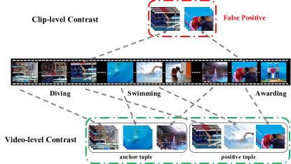
Figure 1: Random sampling of clips from a long video may generate false positive pairs. Our proposed video-level contrastive framework based on segments can generate robust positive training pairs and reason the global information.

A key component of contrastive learning is to define positive and negative samples to contrast. For example, in the image domain, most approaches use random crops from the same image as a positive pair and consider other images in the dataset as negative samples [69, 29, 9]. For video, there are several widely adopted formulations. (i) Instance-based methods [21, 73, 52, 27] use random frames/clips from the same video as a positive pair. (ii) Pace-based methods [63, 72] use clips from the same video but with different sampling rates as a positive pair. (iii) Prediction-based methods [25, 26] use predictions from auto-regressed and ground-truth features at the same spatiotemporal location as a positive pair. However, all previous methods define positive pairs to perform contrastive learning on frame-level or clip-level, which do not capture the global context of a video in long temporal range. In addition, random sampling of clips from an untrimmed video may generate false positive pairs as shown in Fig. 1 top.

In this paper, we propose a new formulation for generating positive pairs to address the above limitation. As shown in Fig. 1 bottom, we first uniformly divide the video into several segments, and randomly pick a clip from each segment to form the anchor tuple. Then we randomly pick a clip from each segment again to form the positive tuple. We consider these two tuples as a positive pair, and tuples from other videos as negative samples. In this way, our formulation of positive samples is flexible (i.e., can be trained on any videos regardless of duration or sampling rate) and is able to reason about the global information across a video. However, global context alone is not enough to guide the unsupervised video representation learning since it does not enforce the inherent sequential structure of a video. Hence, we introduce a regularization loss based on the temporal order constraint. To be specific, we shuffle the frame order inside each tuple and ask the model to predict if the tuple has the correct temporal order. Since both proposed techniques work on the video-level, we term our method as VCLR, video-level contrastive learning. Our contributions can be summarized as follows.

• We introduce a new way to formulate positive pairs based on segments for video-level contrastive learning.

• We incorporate a temporal order regularization term to enforce the inherent sequential structure of videos.

• Our proposed video-level contrastive learning framework (VCLR) outperforms previous literature on five datasets for downstream action classification, action localization and video retrieval.

2 Related Work

Self-supervised image representation learning Initial attempts for self-supervised image representation learning are via designing various pretext tasks. Recently, a type of contrastive learning method based on instance discrimination has taken-off as it has been consistently demonstrated to outperform its supervised counterparts on downstream tasks [11, 10, 23, 7]. The core idea behind contrastive learning is to learn representations by distinguishing between similar and dissimilar instances [69]. More specifically, it obtains the supervision signal by designing different forms of positive and negative pairs, such as random crops from the same image [29, 9], different views of the same instance [55], etc.

Self-supervised video representation learning Compared with images, videos have another axis, temporal dimension, which we can use to craft pretext tasks for self-supervised representation learning. There are many previous attempts [78] including predicting the future [57, 58, 46, 15], predicting the correct order of shuffled frames [48, 19] or video clips [40, 71], predicting video rotation [34], solving a space-time cubic puzzle [36], predicting motion and appearance statistics [62], predicting speed [4, 74] and exploring video correspondence [67, 66, 17, 32]. There is another line of work using multi-modality signals as supervision, such as audio [37, 1, 2, 50, 51] and language [47, 1].

Inspired by the great success of using contrastive learning in image domain, several recent work have considered it in video domain. Despite their loss objectives are similar (e.g., NCE [56] and its variant), their major differences lie in how they formulate positive and negative samples. CBT [12] adapts masked language modeling [14] to a video sequence, and uses the video clip and its masked version as a positive pair. DPC [25] and MemDPC [26] use predictions from autoregressed and ground-truth features at the same spatiotemporal location as a positive pair. Pace [63] and VTHCL [72] proposes to use video clips of the same action instance but with different visual tempos as a positive pair. CMC [55] introduces two ways of sampling positive pairs: (1) different frames from the same video and (2) RGB and flow data of the same frame. Similar to CMC, VINCE [21] and SeCo [73] also use different frames from the same video, while CVRL [52] use different clips from the same video as positive samples. There are also many concurrent work [60, 8, 49, 61, 18, 24, 31, 59].

Different from previous approaches, our work proposes a new way to formulate positive pairs based on segments. Given our formulation, we can perform contrastive learning on video-level rather than frame- or clip-level, and achieve promising results both quantitatively and qualitatively. In addition, our method is generally applicable to various network architectures, and orthogonal to other advancements in self-supervised video representation learning domain.

3 Methodology

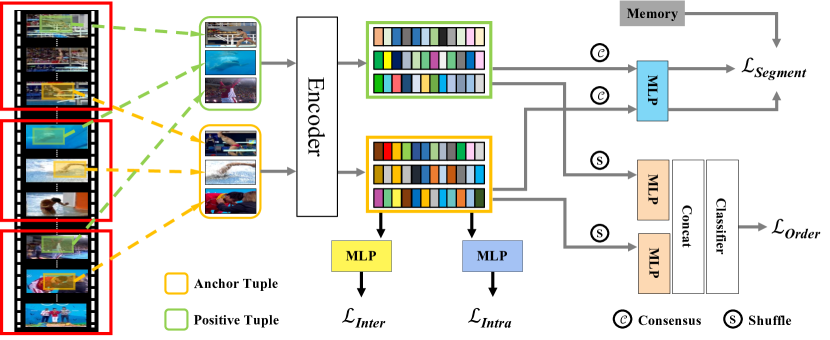
Figure 2: Overview of the proposed VCLR framework. We introduce a new way to formulate positive training pairs based on video segments. There are four loss objectives, $\mathcal{L}_{\textit{Inter}}$ and $\mathcal{L}_{\textit{intra}}$ following [73], and two new ones $\mathcal{L}_{\textit{Segment}}$ and $\mathcal{L}_{\textit{Order}}$ for video-level contrastive learning. Image is best viewed in color.

3.1 Preliminary

Before diving into our proposed framework, we first revisit the concept of contrastive learning in image domain [69, 29, 9]. Here we use MoCoV2 [11] as an illustrating example. More formally, given a set of images $\mathcal{X}$, an image $x_{i}$ is sampled from $\mathcal{X}$ and is augmented to generate a positive pair $x^{a}_{i}$ and $x^{+}_{i}$. A set of negative samples $\mathcal{N^{-}}$ are then selected from the rest of $\mathcal{X}$, i.e., $x_{j}\in\mathcal{N^{-}},j\neq i$. Two encoders, query encoder $f_{q}$ and key encoder $f_{k}$, are used to obtain the visual representations, e.g., 2048-dim features from ResNet50 backbone. These visual representations are then projected via MLP heads $g_{q}$ and $g_{k}$ to lower dimensional embeddings for similarity comparison. For notation simplicity, we represent anchor embedding as $q=g_{q}(f_{q}(x^{a}_{i}))$, positive embedding as $p=g_{k}(f_{k}(x^{+}_{i}))$, and negative embeddings as $n_{j}=g_{k}(f_{k}(x^{-}_{j}))$. At this point, the problem is formulated as a (N+1)-way classification task, and can be optimized by InfoNCE loss [56] as

$$\mathcal{L}_{\text{NCE}}(q,p,\mathcal{N^{-}})=-\log\frac{e^{\text{sim}(q,p)}}{e^{\text{sim}(q,p)}+\sum_{j=1}^{N}e^{\text{sim}(q,n_{j})}}.$$ (1)

Here, sim($\cdot$) is the distance metric used to measure the similarity between feature embeddings, e.g., dot product. $N$ denotes the number of negative samples. By optimizing the objective, the model learns to map similar instances closer and dissimilar instances farther apart in the embedding space. For more details, we refer the readers to [29, 11].

To adapt contrastive learning into video domain, we need to find a way to define positive and negative samples. We have mentioned several in Sec. 2. In this paper, we follow a recent state-of-the-art SeCo [73] as our baseline given their strong performance. Specifically, they introduce two ways to formulate positive and negative samples: inter-frame and intra-frame instance discrimination.

Inter-frame instance discrimination Unlike approaches in image domain that take random crops from the same image as a positive pair, inter-frame instance discrimination simply treats random frames from the same video as positive. Suppose we randomly pick three frames from a video, $v_{1},v_{2}$ and $v_{3}$, inter-frame instance discrimination task considers $v^{a}_{1}$ as the anchor frame, $(v^{+}_{1},v_{2},v_{3})$ as the positive samples, and frames from other videos in the dataset as negative samples $\mathcal{N^{-}}$. Here, $v^{a}_{1}$ and $v^{+}_{1}$ are generated from $v_{1}$ by different augmentations. Mathematically, the loss objective can be written as

$$\mathcal{L}_{\textit{Inter}}=\frac{1}{3}\sum\mathcal{L}_{\text{NCE}}(q_{1}^{a},\{p_{1}^{+},p_{2},p_{3}\},\mathcal{N^{-}}).$$ (2)

We represent anchor embeddinig as $q_{1}^{a}=g_{q}^{e}(f_{q}(v^{a}_{1}))$, and positive embeddings as $p_{1}^{+}=g_{k}^{e}(f_{k}(v^{+}_{1}))$, $p_{2}=g_{k}^{e}{}(f_{k}(v_{2}))$, $p_{3}=g_{k}^{e}(f_{k}(v_{3}))$. $g_{q}^{e}$ and $g_{k}^{e}$ are MLP heads for inter-frame instance discrimination task. Note that, we have multiple positives in Eq. (2), we compute the contrastive losses separately and take their average.

Intra-frame instance discrimination In order to learn better appearance representation, intra-frame instance discrimination is adopted to explore the inherently spatial changes across frames. Different from inter-frame, we only use $v^{+}_{1}$ as a positive sample, and consider $v_{2}$, $v_{3}$ as negative samples. Hence, the loss objective can be written as

$$\mathcal{L}_{\textit{Intra}}=\mathcal{L}_{\text{NCE}}(q^{a}_{1},\{p_{1}^{+}\},\{p_{2},p_{3}\}).$$ (3)

Essentially, this task is the same as standard instance discrimination in image domain except trained with a much smaller negative set. The embeddings in Eq. (3) are actually different from the ones in Eq. (2) due to using different MLP heads $g_{q}^{r}$ and $g_{k}^{r}$ for intra-frame instance discrimination task, but we reuse them for notation simplicity.

Despite the design of both inter- and intra- frame instance discrimination task, SeCo still performs contrastive learning on the frame-level. Simply put, intra-frame is between two crops in the same image, and inter-frame is between two frames in the same video. Some recent work [27, 52] use short video clips as input to perform instance discrimination, which can be considered doing contrastive learning in the clip-level. However, contrastive learning on frame- or clip-level are sub-optimal for video representation learning because they cannot capture the evolving semantics in the temporal dimension. Hence, we ask the question, how can we perform contrastive learning in the video-level?

3.2 Video-level contrastive learning

Long-range temporal structure plays an important role in understanding the dynamics in videos. In terms of supervised learning, there have been a series of work to explore global context [64, 16, 20, 65, 77, 68, 75, 41, 42]. However, in terms of self-supervised learning, few efforts have been done to incorporate global video-level information.

In this work, inspired by [64, 39], we propose to use the segment idea to sample positive pairs for contrastive learning. Formally, given a video $V$, we divide it into $K$ segments $\{S_{1},S_{2},\cdots,S_{K}\}$ of the equal duration. Within each segment $S_{k}$, we randomly sample a frame $v_{k}$ to formulate our anchor tuple, i.e., $t^{a}=\{v_{1}^{a},v_{2}^{a},\cdots,v_{K}^{a}\}$. Then, we take a second independent random sample of $K$ frames in the same manner to formulate the positive tuple, $t^{+}=\{v_{1}^{+},v_{2}^{+},\cdots,v_{K}^{+}\}$. We consider these two tuples as a positive pair, because both of them describe the evolving semantics inside a video. Intuitively, segment-based sampling can be considered as a form of data augmentation, so that the consensus from two tuples can produce two different views of the same video, which is what instance discrimination need to learn an effective representation.

In terms of loss objective, each frame in the tuple will produce its own preliminary frame-level representation. Then a consensus among these representations will be derived as the video-level representation. The final embedding of the anchor and positive tuple can be represented as

$$q_{t}^{a}=g_{q}^{s}(\mathcal{C}[f_{q}(v_{1}^{a}),f_{q}(v_{2}^{a}),...,f_{q}(v_{K}^{a})])$$ (4)

$$p_{t}^{+}=g_{k}^{s}(\mathcal{C}[f_{k}(v_{1}^{+}),f_{k}(v_{2}^{+}),...,f_{k}(v_{K}^{+})])$$ (5)

where $\mathcal{C}$ denotes the consensus operation, e.g., average. $g_{q}^{s}$ and $g_{k}^{s}$ are MLP heads for video-level instance discrimination task. Once we have the embeddings $q_{t}^{a}$ and $p_{t}^{+}$, we can compute the video-level contrastive loss as

$$\mathcal{L}_{\textit{segment}}=\mathcal{L}_{\text{NCE}}(q_{t}^{a},p_{t}^{+},\mathcal{N^{-}}).$$ (6)

Here, we reuse the notation $\mathcal{N^{-}}$ to generally indicate the negative set, where each negative is a tuple of frames sampled from other videos in the dataset.

We want to point it out that, this formulation of positive samples has several advantages. First, it leads to a more robust training as it sees information from the entire video. Second, we can use this strategy to train a model on any types of video, regardless of duration or sampling rate. Third, this formulation is not limited to video frames with 2D CNNs, but also ready to be used for video clips with 3D CNNs. In addition, our formulation is orthogonal to other advancements in self-supervised video representation learning [72, 27, 25], which could be incorporated seamlessly.

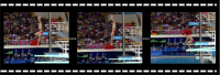
(a)

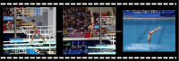
(b)

Figure 3: Left: It is challenging to identify the temporal order within a local sequence, which will likely confuse the model training. Right: With longer temporal context, we can easily tell the evolution of events.

Method	Network	Top-1 Acc. (%)
VTHCL [72]	R3D-50	37.8
VINCE [21]	R2D-50	49.1
SeCo [73]	R2D-50	61.9
VCLR	R2D-50	64.1
Sup-ImageNet	R2D-50	52.3
Sup-Kinetics400	R2D-50	69.9

Table 1: Linear evaluation on Kinetic400. Our method outperforms previous methods and is close to supervised upper bound. Sup-ImageNet:supervised ImageNet weights. Sup-Kinetics400: supervised training on Kinetics400.

3.3 Temporal order regularization

Video-level contrastive learning helps to capture global context as it sees information from the entire video, but it is weak in enforcing the inherent sequential structure. Given temporal coherence is a strong constraint, there has been some work [48, 19, 40, 73] that use it as a supervision signal for self-supervised video representation learning.

In this paper, we also use the temporal order as a regularization term under our contrastive learning framework. To be specific, given tuples $t^{a}$ and $t^{+}$, which are sampled based on segments described in Sec. 3.2, we randomly shuffle the frames inside each tuple with $50\%$ chance. This will lead to a balanced 4-way classification problem: both tuples are in correct temporal order, $t^{a}$ correct and $t^{+}$ shuffled, $t^{a}$ shuffled and $t^{+}$ correct, and both shuffled.

In terms of loss objective, we first compute the embeddings of each tuple as $o_{t}^{a}$ and $o_{t}^{+}$,

$$o_{t}^{a}=[g_{q}^{o}(f_{q}(v_{1}^{a})),g_{q}^{o}(f_{q}(v_{2}^{a})),...,g_{q}^{o}(f_{q}(v_{K}^{a}))]$$ (7)

$$o_{t}^{+}=[g_{k}^{o}(f_{k}(v_{1}^{+})),g_{k}^{o}(f_{k}(v_{2}^{+})),...,g_{k}^{o}(f_{k}(v_{K}^{+}))]$$ (8)

$g_{q}^{o}$ and $g_{k}^{o}$ are MLP heads for temporal order regularization. In order to keep the temporal order within each tuple, we concatenate the embeddings and predict its order type,

$$y^{*}=h_{o}([\text{concat}(o_{t}^{a}),\text{concat}(o_{t}^{+})]).$$ (9)

Here, $h_{o}$ is a linear classifier to project the concatenated embeddings to logits. $y^{*}$ is the order type prediction, i.e., class 0, 1, 2 or 3. In the end, we compute the cross-entropy loss between the predictions and pre-defined ground-truth

$$\mathcal{L}_{\textit{Order}}(y,y^{*})=-\sum y\log y^{*}.$$ (10)

Our temporal order regularization may seem similar to [19, 40], but we build it upon our video-level sampling framework. Simply put, previous approaches use local sequence to validate temporal order, while we use global sequence. One drawback of using local sequence is that it may not provide enough cues to predict the correct sequential structure. As shown in Fig. 3 left, any temporal order seems reasonable between these three frames sampled from a local sequence. On the contrary in Fig. 3 right, using our video-level sampling strategy, it is less ambiguous to determine the temporal order inside a tuple.

3.4 Overall framework

At this point, we present our video-level contrastive learning method, VCLR, for self-supervised video representation learning. Our overall framework can be seen in Fig. 2. During training, the final loss objective is a summation of previous four loss objectives,

$$\mathcal{L}=\mathcal{L}_{\textit{Inter}}+\mathcal{L}_{\textit{Intra}}+\mathcal{L}_{\textit{Segment}}+\mathcal{L}_{\textit{Order}}$$ (11)

For downstream tasks, we ignore the MLP heads designed for each task, e.g., $g^{e}$, $g^{r}$, $g^{s}$ and $g^{o}$. We only use pretrained encoder $f_{q}$ for extracting features or finetuning.

4 Experiments

4.1 Datasets

We conduct experiments on 5 datasets, Kinetics400 [35], UCF101 [54], HMDB51 [38], Something-Something-v2 [22] and ActivityNet [6]. Kinetics400 consists of approximately 240k training and 20k validation videos trimmed to 10 seconds from 400 human action categories. UCF101 contains $13,320$ videos spreading over 101 categories of human actions. HMDB51 contains $6,849$ videos divided into 51 action categories. Something-Something-v2 consists of 174 action classes and a total of $220,847$ videos. For notation simplicity, we refer this dataset as SthSthv2 for the rest of the paper. ActivityNet (V1.3) contains 200 human daily living actions. It has $10,024$ training and $4,926$ validation videos. Both UCF101 and HMDB51 have three official train-val splits, and we report performance on its split 1 for fair comparison to previous work. For other three datasets, we report performance on their validation sets.

Method	Venue	Network	Top-1 Acc (%)
			UCF101	HMDB51
ST-Puzzle [36]	AAAI19	R3D-50	65.8	33.7
MAS [62]	CVPR19	C3D	61.2	33.4
DPC [25]	ICCVW19	R-2D3D	75.7	35.7
SpeedNet [4]	CVPR20	S3D-G	81.1	48.8
VIE [79]	CVPR20	SlowFast	80.4	52.5
MemDPC [26]	ECCV20	R-2D3D	78.1	41.2
PacePred [63]	ECCV20	R(2+1)D	77.1	36.6
TT [33]	ECCV20	R3D-18	79.3	49.8
SeCo[73]	AAAI21	R2D-50	83.4	49.7
VCLR	-	R2D-50	85.6	54.1
Sup-ImageNet	-	R2D-50	81.6	49.0
Sup-Kinetics400	-	R2D-50	88.1	56.1

Table 2: Downstream action classification on UCF101 and HMDB51. Sup-Kinetics400: supervised Kinetics400 pretrained weights.

Method	Video Algorithm	Top-1 Acc (%)
VINCE [21]	TSN	31.4
	TSM	50.3
SeCo [73]	TSN	31.9
	TSM	50.7
VCLR	TSN	33.3
	TSM	52.0
Sup-ImageNet	TSN	33.0
	TSM	59.1

Table 3: Downstream action classification on SthSthv2. TSM: temporal shift module network [43]. All methods in this table use R2D-50 as encoder, and follow the same training setting for fair comparison.

Method	Modality	Network	Pretrain	UCF101				HMDB51
				R@1	R@5	R@10	R@20	R@1	R@5	R@10	R@20
OPN [40]	V	VGG	UCF101	19.9	28.7	34.0	40.6	-	-	-	-
DRL [5]	V	VGG	UCF101	25.7	36.2	42.2	49.2	-	-	-	-
VCOP [71]	V	R(2+1)D	UCF101	14.1	30.3	40.4	51.1	7.6	22.9	34.4	48.8
VCP [45]	V	R3D-50	UCF101	18.6	33.6	42.5	53.5	7.6	24.4	36.3	53.6
MemDPC [26]	V	R-2D3D	UCF101	20.2	40.4	52.4	64.7	7.7	25.7	40.6	57.7
MemDPC [26]	F	R-2D3D	UCF101	40.2	63.2	71.9	78.6	15.6	37.6	52.0	65.3
CoCLR [27]	VF	S3D	UCF101	53.3	69.4	76.6	82.0	23.2	43.2	53.5	65.5
VCLR	V	R2D-50	UCF101	46.8	61.8	70.4	79	17.6	38.6	51.1	67.6
SpeedNet [4]	V	S3D-G	Kinetics400	13.0	28.1	37.5	49.5	-	-	-	-
SeCo [73]	V	R2D-50	Kinetics400	69.5	79.5	85	90.1	33.6	57.4	67.6	78.6
VCLR	V	R2D-50	Kinetics400	70.6	80.1	86.3	90.7	35.2	58.4	68.8	79.8

Table 4: Downstream video retrieval on UCF101 and HMDB51. V: RGB frames. F: optical flow.

Method	Classification	Localization
	Top-1 Acc (%)	AUC (%)	AR@100 (%)
VINCE [21]	60.7	64.6	73.2
SeCo [73]	67.8	65.2	73.4
VCLR	71.9	65.5	73.8
Sup-ImageNet	67.2	64.8	73.4

Table 5: Downstream action classification and localization on ActivityNet. All methods use R2D-50 as encoder, and follow the same training setting for fair comparison.

4.2 Implementation details of pretraining

In terms of input, we follow our segment-based sampling strategy to choose two tuples from the same video as video-level anchor and positive sample. We set the number of segments to $3$, i.e., each tuple contains three frames. The video-level anchor will also be used to generate frame-level anchor and positive sample to compute the inter-frame and intra-frame losses. For data augmentation, we apply random scales, color-jitter, random grayscale, random Gaussian blur, and random horizontal flip. In terms of network architecture, we use ResNet50 [30] as our backbone, plus four MLP heads designed for each loss. We use average operation for $\mathcal{C}$. In terms of optimization, we train the model on Kinetics400 dataset with a batch size of $512$ for $400$ epochs following [73]. We use SGD to optimize the network with an initial learning rate of $0.2$, and annealed to zero with a cosine decay scheduler. More details can be found in the Appendix Sec A.

4.3 Linear evaluation on Kinetics400

In order to quantify the quality of learned representation, the most straightforward way is to treat the pretrained model as a feature extractor and train a classifier on top of the features to see its generalization performance.

Following [73], we uniformly sample 30 frames from each video, resize each frame with short edge of 256 and center-crop it to $224\times 224$. We forward each frame through the frozen ResNet50 backbone, get the frame-level features and average them into video-level feature. A linear SVM is then trained on the video-level features of the Kinetics400 training set, and finally evaluated on its validation set.

As we can see in Table 1, our method outperforms previous literature in terms of linear evaluation on Kinetics400 dataset. Especially for fair comparison when using 2D ResNet50, our VCLR pretrained model is $11.8\%$ higher than ImageNet pretrained weights, and $2.2\%$ higher than previous state-of-the-art SeCo pretrained weights [73]. In addition, we further close the gap between unsupervised feature learning and supervised upper bound ($64.1\%$ vs $69.9\%$). This clearly demonstrates the effectiveness of performing contrastive learning on video-level. We note that a recent work CVRL [52] performs slightly better than us. However, we conjecture it is because CVRL has been trained with a heavier architecture (3D ResNet50 [28] with 31.7M parameters) and twice our epochs (800).

4.4 Downstream action classification

A main goal of unsupervised learning is to learn features that are transferable [29]. In both computer vision and natural language processing, pretraining a network on large datasets and finetuning it on smaller datasets is the de facto way to achieve promising results on downstream tasks.

Following previous work [26, 73], we transfer our pretrained backbone and finetune all its layers on UCF101 and HMDB51 datasets. We compare our method to recent literature in Table 2. Note that there are more related work, but we only list methods that are pretrained on Kinetics400 and using RGB frames as input for fair comparison. A complete comparison including models trained on larger datasets [15] or multi-modality [27] can be found in the Appendix Table 11. As can be seen in Table 2, our method with 2D ResNet50 is able to outperform those using more advanced 3D CNNs [79, 4]. Compared to previous state-of-the-art SeCo [73], we find that video-level contrastive learning brings $2.2\%$ and $4.4\%$ absolute performance improvement on UCF101 and HMD51, respectively. Similarly, our VCLR pretrained models achieve higher accuracy than ImageNet pretrained weights on both datasets, and perform very close to Kinetics400 pretrained weights.

In order to have a complete understanding of our learned representation’s transferrability, we further evaluate VCLR on another two popular action classification datasets, SthSthv2 and ActivityNet. This is because UCF101 and HMDB51 have small domain gap to Kinetics400, given they are all scene-focused datasets, e.g., most actions can be predicted correctly by using object or background prior. SthSthv2 is a motion-focused dataset and requires strong temporal reasoning because most activities cannot be inferred based on spatial features alone (e.g. opening something, covering something with something). ActivityNet contains long and untrimmed videos, and thus requires strong global context modeling.

In terms of SthSthv2, we compare our learned representations to those from VINCE and SeCo in Table 3. As we can see, our learned representation achieves higher accuracy than both of them. We also show that our pretrained backbone is compatible with different video action recognition algorithms. Besides TSN [64], we adapt our pretrained weights to initialize a popular algorithm TSM [43] on SthSthv2 and obtain promising results. In terms of ActivityNet, we also compare our learned representations to those from VINCE and SeCo in Table 5 and show significant performance improvements.

To summarize, by performing contrastive learning on video-level, our proposed VCLR is able to outperform previous state-of-the-art approaches on 4 downstream action classification datasets, including scene-focused datasets (UCF101 and HMDB51), motion-focused dataset (SthSthv2) and untrimmed video dataset (ActivityNet).

4.5 Downstream action temporal localization

We also evaluate VCLR on action temporal localization task with ActivityNet. The goal of this task is to generate high quality proposals to cover action instances with high recall and high temporal overlap. To be specific, we adopt the popular BMN [44] method for action localization, and only change the input features to see which representation generalizes better. To evaluate proposal quality, Average Recall (AR) under multiple IoU thresholds are calculated. We calculate AR under different Average Number of proposals (AN) as AR@AN, and calculate the Area under the AR vs. AN curve (AUC) as metrics, where AN is varied from 0 to 100. As can be seen in Table 5, our VCLR learned representations not only outperforms previous methods by a large margin on classification task, it also performs better on action localization. Qualitatively, we show two visualizations of our predicted proposals in Fig. 4b.

4.6 Downstream video retrieval

In addition to action classification and localization, we also evaluate VCLR on a common downstream task, video retrieval. For this task, we use the extracted feature from each video to perform nearest-neighbour retrieval, and the goal is to test if the query clip instance and its nearest neighbours belong to same semantic category. Similar to linear evaluation in Sec. 4.3, we treat the pretrained model as a feature extractor, and no finetuning is performed.

Following [71, 27], we use the validation video samples in UCF101 and HMDB51 to search the $k$ nearest video samples from their training sets, respectively. We use Recall at $k$ (R$@k$) as evaluation metric, that means if one of the top $k$ nearest neighbours is from the same class as query, it is a correct retrieval. As can be seen in Table 4, our VCLR trained representation outperforms other methods with respect to all the R$@k$ regardless of the pretraining dataset. Qualitatively, we show several visualizations of our top-3 video retrievals on UCF101 dataset in Fig. 4a. We note that a recent work CoCLR [27] performs better than us. However, CoCLR has been trained with a heavier network S3D [70] and multiple hard positive samples mined by using optical flow. We conduct another experiment in Sec. 5.3 to fairly compare with CoCLR using the same network architecture, and find that our performance is competitive to theirs even without using optical flow.

$\mathcal{L}_{\textit{Intra}}$	$\mathcal{L}_{\textit{Inter}}$	$\mathcal{L}_{\textit{Segment}}$	$\mathcal{L}_{\textit{Order}}$	Top-1 Acc. (%)
✓				NA
	✓			59.0
		✓		62.1
			✓	51.8
✓	✓			60.7
✓	✓		✓	61.2
✓	✓	✓		63.5
✓	✓	✓	✓	64.1

Table 6: Ablation study on loss objectives. We prertain all configurations on Kinetics400 under the same setting, and report linear evaluation performance on it.

Num. of Segments ($K$)	Top-1 Acc. (%)
$K=1$	61.2
$K=2$	63.0
$K=3$	64.1
$K=4$	64.3
$K=5$	64.4

Table 7: Ablation study on the number of segments. We report the linear evaluation performance here.

Method	Modality	Retrieval	Classification
			Linear	Finetune
$\mathcal{L}_{\textit{Inter}}$ [27]	V	33.1	46.8	78.4
$\mathcal{L}_{\textit{Inter}}$ + $\mathcal{L}_{\textit{Segment}}$	V	49.8	67.4	80.2
$\mathcal{L}_{\textit{Inter}}$ + $\mathcal{L}_{\textit{Segment}}$ + $\mathcal{L}_{\textit{Order}}$	V	51.7	70.9	81.7
CoCLR [27]	VF	51.8	70.2	81.4

Table 8: VCLR with 3D CNNs. All models are pretrained on UCF101 under the same setting following [27].

Method	Pretrain	Classification
		UCF101	HMDB51
DPC [25]	UCF101	60.6	44.9
DPC + $\mathcal{L}_{\textit{Segment}}$	UCF101	62.0	46.3
DPC + $\mathcal{L}_{\textit{Segment}}$ + $\mathcal{L}_{\textit{Order}}$	UCF101	62.7	47.1

Table 9: VCLR with DPC [25]. All models are pretrained under the same setting following [25].

Method	Pretrain	Classification
		UCF101	HMDB51
SeCo [73]	HACS	64.1	47.2
PacePred [63]	HACS	62.8	46.6
DPC [25]	HACS	60.1	45.4
VCLR	HACS	67.2	49.3

Table 10: Pretrain on multi-label dataset HACS [76]. All methods use R3D-18 for fair comparison.

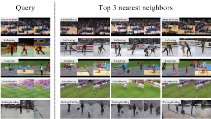
(a)

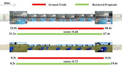
(b)

Figure 4: (a) Video retrieval results on UCF101. (b) Action localization results on ActivityNet. For both experiments, we use the learned representations from our VCLR model pretrained on Kinetics400 dataset.

5 Discussion

In this section, we present ablation studies and important discussions on VCLR. Given space limitation, we put more experiments, visualizations and implementation details in the supplemental materials.

5.1 Ablation study on loss objectives

Our method VCLR has four loss objectives: $\mathcal{L}_{\textit{Intra}}$, $\mathcal{L}_{\textit{Inter}}$, $\mathcal{L}_{\textit{Segment}}$ and $\mathcal{L}_{\textit{Order}}$. We now dissect their contributions and see how they impact the learned representations.

We have several observations from Table 6. First, video-level instance discrimination $\mathcal{L}_{\textit{Segment}}$ is a strong supervision signal. By using this loss alone could learn good representations and outperform previous state-of-the-art SeCo ($62.1$ vs $61.9$). Second, temporal order constraint $\mathcal{L}_{\textit{Order}}$ is relatively weak. Using it alone only achieves $51.8\%$ accuracy. However, when combined with other loss objectives, it can provide further regularization and push the performance to $64.1$. Third, using intra-frame instance discrimination $\mathcal{L}_{\textit{Intra}}$ alone is not enough to stabilize training as the negative set is too small to perform contrasting.

5.2 Ablation study on the number of segments

We set $K=3$ as default number of segments in our experiments, now we discuss the impact of the number of segments for our method. We present the comparisons with respect to linear evaluation performance on Kinetics400 dataset in Table 7.

We can see that with the increasing number of segments, the performance continue to improve, which indicates the necessity of using global context in training video models. However, the performance starts to saturate when using more segments. In our paper, we simply choose $K$=$3$ for a better training speed-accuracy trade-off.

5.3 General applicability

Our framework VCLR is not limited to any network architecture. For example, we could sample short video clips instead of frames from each segment to formulate positive pairs. In this way, a 3D CNN can be pretrained without using labels. In addition, VCLR is compatible with most loss objectives, and is orthogonal to other advancements in self-supervised video representation learning.

VCLR with 3D CNNs Here we train a R3D-50 model using VCLR to demonstrate our framework’s general applicability. In terms of baseline, we compare to a R3D-50 model pretrained by $\mathcal{L}_{\textit{Inter}}$ on UCF101 dataset following [27]. We then use three segments and pretrain the model by adding loss objectives $\mathcal{L}_{\textit{Segment}}$ and $\mathcal{L}_{\textit{Order}}$. As seen in Table 8, our method significantly outperforms the corresponding baseline with respect to both video classification and retrieval task on UCF101. In addition, we compare to CoCLR [27], which uses optical flow to mine multiple hard positives for contrastive learning. We can see that our method is competitive to CoCLR even without optical flow.

VCLR with DPC Both $\mathcal{L}_{\textit{Segment}}$ and $\mathcal{L}_{\textit{Order}}$ are compatible to other algorithms in self-supervised video representation learning. Similarly, we incorporate them to a recent work DPC [25], which uses dense prediction as a pretext task, to train a R3D-18 model on UCF101. As shown in Table 9, a simple addition improves the transfer performance to downstream action classification task on both UCF101 and HMDB51, which demonstrates the necessity of using global context. We believe VCLR can be combined with other methods [72, 52] and show performance improvements.

5.4 Visualization

We visualize the activations of the conv5 output from ResNet50 models pretrained by SeCo [73] and ours. As can be seen in Fig. 5, VCLR is able to focus on the moving region of interest, while SeCo focuses more on the background (e.g., springboard and water). It is also interesting to note that VCLR generalizes better to unseen videos.

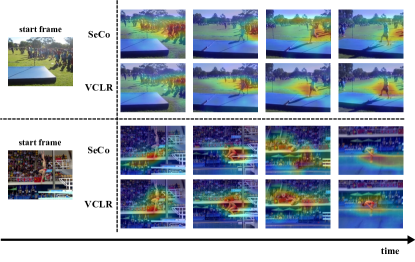
Figure 5: Attention visualization between SeCo [73] and VCLR. The upper video is from Kinetics400 validation set, and the bottom one is an unseen video from Internet.

5.5 Pretrain on multi-label videos

As aforementioned, our framework is able to generate robust positive pairs for contrastive learning compared with clip-level sampling strategy. However, we conduct all experiments by pretraining the model on Kinetics400 dataset in order to perform fair comparison with previous literature. Here we pretrain the model on a multi-label dataset, HACS [76], to demonstrate the advantage of VCLR.

We compare VCLR to three methods, SeCo [73], PacePred [63] and DPC [25]. They correspond to the three different ways of formulating positive pairs as mentioned in Sec. 1, namely instance-based, pace-based and prediction-based contrastive learning. We use the same backbone R3D-18, and perform finetuning on UCF101 to evaluate the quality of learned representations. As seen in Table 10, our VCLR outperforms them by a large margin, which indicates the importance of generating correct positive pairs and the necessity of using global context.

6 Conclusion

In this paper, we introduce a new way to formulate positive pairs for video-level contrastive learning. We also incorporate a temporal order regularization to enforce the inherent sequential structure of videos during training. Our final framework VCLR shows state-of-the-art results on five video datasets for downstream action recognition/localization and video retrieval. Furthermore, we demonstrate the generalization capability of our method, e.g., pretrain 3D CNNs and compatible with other self-supervised learning algorithms. We want to emphasize that the effectiveness of VCLR is beyond the experimental results presented in this paper due to using trimmed video datasets for the sake of fair comparison. Our method is applicable to various inputs (short trimmed or long untrimmed videos), networks (2D or 3D CNNs), methods (various algorithms) and ready to scale to future datasets for video self-supervised representation learning. We hope VCLR can serve as a strong baseline and facilitate research of using global context for video understanding.

In the appendix, we provide more implementation details, performance comparisons and visualizations. Specifically, we first describe the implementation details of experiments on pretraining, downstream tasks and discussions in Sec. A. We then present a complete comparison to other published methods in terms of downstream action classification in Sec. B. In the end, we show more visualizations of our successful predictions, failure cases and feature visualizations in Sec. C.

Appendix A Implementation Details

A.1 Pretraining setup

Our query encoder $f_{q}$ is a ResNet50 model. Following [11, 73], we also have a key encoder $f_{k}$ (a.k.a, momentum encoder) which has the same architecture as $f_{q}$ but updated with a momentum strategy,

$$f_{k}^{t}=mf_{k}^{t-1}+(1-m)f_{q}^{t-1}.$$ (12)

Here, $t$ indicates the training iteration step. We set the momentum $m$ to $0.999$. The anchor samples are always encoded by query encoder $f_{q}$. Both positive and negative samples are encoded by key encoder $f_{k}$. The negative samples are stored in a memory bank. We have two memory banks, one for video-level contrastive loss $\mathcal{L}_{\textit{Segment}}$, the other for inter-frame contrastive loss $\mathcal{L}_{\textit{Inter}}$. Both memory banks have a size of $131,072$, following SeCo [73]. Since we have four loss objectives, we have four MLP heads after the backbone encoder. All four MLP heads have the same architecture, but do not share weights. Specifically, each head consists of a fully-connected layer ($2048\times 2048$), a ReLU activation layer and a final embedding layer ($2048\times 128$). All the embeddings are then L2-normalized before computing the loss objectives. The overall loss is a simple summation over four losses. We did not do parameter tuning on the loss weights, although weighted summation might lead to improved performance. We note that these four MLP heads are only used during training, but discarded for downstream tasks. In terms of optimization, we train the model on Kinetics400 dataset with a batch size of 512 for 400 epochs. We also employ the Shuffle-BN for multi-GPU training as in [29]. We use SGD to optimize the network with an initial learning rate of $0.2$, and annealed to zero with a cosine decay scheduler. During linear evaluation, the ResNet50 backbone is frozen and treated as a feature extractor. We train a linear SVM  with the Kinetics400 training set and report performance on its validation set.

A.2 Downstream setup

For all the downstream tasks, we adopt mmaction2 [13] toolkit and mostly follow their default settings to perform finetuning on each dataset.

A.2.1 Action classification

UCF101

We use the pretrained ResNet50 as backbone network initialization and finetune it on UCF101 dataset. During training, we uniformly divide each video into 3 segments, and select one frame from each segment. For data augmentation, we apply random resized cropping, random horizontal flip, and then resize it to $224\times 224$. We use average operation for taking consensus $\mathcal{C}$ following TSN [64]. We use SGD to optimize the model for $300$ epochs with a batch size of $256$. The initial learning rate is set to $0.01$, and decayed by $0.1$ at $120$ and $240$ epoch respectively. The momentum is $0.9$ and the weight decay is $5\times 10^{-4}$. During test, we uniformly sample 25 frames from each video, perform center crop to $224\times 224$ and average their predictions to be the final video prediction.

HMDB51

We use the pretrained ResNet50 as backbone network initialization and finetune it on HMDB51 dataset. During training, we uniformly divide each video into 8 segments, and select one frame from each segment. For data augmentation, we apply random resized cropping, random horizontal flip, and then resize it to $224\times 224$. We use average operation for taking consensus $\mathcal{C}$ following TSN [64]. We use SGD to optimize the model for $50$ epochs with a batch size of $256$. The initial learning rate is set to $0.025$, and decayed by $0.1$ at $20$ and $40$ epoch respectively. The momentum is $0.9$ and the weight decay is $1\times 10^{-4}$. During test, we uniformly sample 8 frames from each video, perform center crop to $224\times 224$ and average their predictions to be the final video prediction.

SthSthV2

We use the pretrained ResNet50 as backbone network initialization and finetune it on SthSthV2 dataset. During training, we uniformly divide each video into 8 segments, and select one frame from each segment. For data augmentation, we apply multi-scale cropping with scales $\{1,0.875,0.75,0.066\}$, random horizontal flip, and then resize it to $224\times 224$. We use average operation for taking consensus $\mathcal{C}$ following TSN [64]. We use SGD to optimize the model for $50$ epochs with a batch size of $128$. The initial learning rate is set to $0.02$, and decayed by $0.1$ at $20$ and $40$ epoch respectively. The momentum is $0.9$ and the weight decay is $1\times 10^{-4}$. During test, we uniformly sample 8 frames from each video, perform 10-crop to $224\times 224$ and average their predictions to be the final video prediction.

We also finetune a recent TSM [43] model for action classification on SthSthV2. We only change the initial learning rate to $0.0075$ , weight decay to $5\times 10^{-4}$, batch size to $48$, the rest setting remain the same as TSN training.

ActivityNet

We use the pretrained ResNet50 as backbone network initialization and finetune it on ActivityNet dataset. During training, we uniformly divide each video into 8 segments, and select one frame from each segment. For data augmentation, we apply random resized cropping, random horizontal flip, and then resize it to $224\times 224$. We use average operation for taking consensus $\mathcal{C}$ following TSN [64]. We use SGD to optimize the model for $50$ epochs with a batch size of $64$. The initial learning rate is set to $0.01$, and decayed by $0.1$ at $20$ and $40$ epoch respectively. The momentum is $0.9$ and the weight decay is $1\times 10^{-4}$. During test, we uniformly sample 25 frames from each video, perform 3-crop to $224\times 224$ and average their predictions to be the final video prediction.

A.2.2 Action localization

For action localization on ActivityNet, we first extract video features from the finetuned ResNet50 model on ActivityNet mentioned above. We then use them to train a recent BMN [44] model to perform action localization. The BMN model is optimized by Adam for 9 epochs with a batch size of 16. The initial learning rate is set to $0.001$ and decayed by $0.1$ at epoch 7.

A.2.3 Video retrieval

For video retrieval, we use the validation video samples in UCF101 and HMDB51 to search the top k nearest neighbors from training set following  [71, 45]. In details, we sample 30 frames of each video, then input them to ResNet50 and employ consensus $\mathcal{C}$ with average operation to get the video features. Then, we search the k nearest neighbors according to the cosine similarity between input video features with each training video.

A.3 Discussion setup

VCLR with 3D CNNs

Following CoCLR [27], we choose the S3D architecture [70] as the backbone for all three experiments. For $\mathcal{L}_{\textit{Inter}}$, we use 32-frame video clip as input. When adding the other two losses, we uniformly divide the video into 3 segments and randomly pick a 32-frame video clip from each segment. Each frame is of size $128\times 128$. We train the model on UCF101 for 300 epochs with a batch size of 64. The initial learning rate is set to $0.001$ and decayed by 10 at epoch 250 and 280.

VCLR with DPC

Following DPC [25], we choose R3D-18 architecture as the backbone for all three experiments. When adding the other two losses, we uniformly divide the video into 3 segments and randomly pick a 5-frame video clip from each segment. Each frame is of size $128\times 128$. We train the model on UCF101 for 300 epochs with a batch size of 128. The initial learning rate is set to $0.001$ and decayed by 10 at epoch 150 and 250.

Method	Venue	Pretraining dataset (duration)	Network	Mod.	Frozen	Top-1 Acc (%)
						UCF101	HMDB51
MemDPC [26]	ECCV2020	K400 (28d)	R-2D3D	V	✓	54.1	30.5
XDC [2]	NeurlPS 2020	IG65M (21y)	R(2+1)D	VA	✓	85.3	56.1
MIL-NCE [47]	CVPR 2020	HTM (15y)	S3D	VT	✓	82.7	53.1
MIL-NCE [47]	CVPR 2020	HTM (15y)	I3D	VT	✓	83.4	54.1
Elo [51]	CVPR 2020	Youtube8M (8y)	I3D	VAF	✓	-	64.5
CoCLR [27]	NeurlPS 2020	K400 (28d)	S3D	VF	✓	77.8	52.4
VCLR		K400 (28d)	R2D-50	V	✓	85.1	51.6
MAS [62]	CVPR 2019	K400 (28d)	C3D	V	✗	61.2	33.4
ST-Puzzle [36]	AAAI 2019	K400 (28d)	R3D-50	V	✗	65.8	33.7
VCOP [71]	CVPR 2019	K400 (28d)	R(2+1)D	V	✗	72.4	30.9
DPC [25]	ICCVW 2019	K400 (28d)	R-2D3D	V	✗	75.7	35.7
DynamoNet [15]	ICCV 2019	Youtube8M-1 (58d)	STCNet	V	✗	88.1	59.9
PacePred [63]	ECCV 2020	K400 (28d)	R(2+1)D	V	✗	77.1	36.6
MemDPC [26]	ECCV 2020	K400 (28d)	R-2D3D	V	✗	78.1	41.2
TT [33]	ECCV 2020	K400 (28d)	R3D-18	V	✗	79.3	49.8
VIE [79]	CVPR 2020	K400 (28d)	SlowFast	V	✗	80.4	52.5
SpeedNet [4]	CVPR 2020	K400 (28d)	S3D-G	V	✗	81.1	48.8
Bi-Pred [3]	WACV 2021	K400 (28d)	R2D-50	V	✗	66.4	45.3
SeCo [73]	AAAI 2021	K400 (28d)	R2D-50	V	✗	83.4	49.7
CVRL [52]	CVPR 2021	K400 (28d)	R3D-50	V	✗	92.9	67.9
MemDPC [26]	ECCV 2020	K400 (28d)	R-2D3D	VF	✗	86.1	54.5
CoCLR [27]	NeurIPS 2020	K400 (28d)	S3D	VF	✗	90.6	62.9
AVTS [37]	NeurIPS 2018	AudioSet (240d)	MC3	VA	✗	89.0	61.6
XDC [2]	NeurIPS 2020	AudioSet (240d)	R(2+1)D	VA	✗	91.2	61.0
XDC [2]	NeurIPS 2020	IG65M (21y)	R(2+1)D	VA	✗	94.2	67.4
MIL-NCE [47]	CVPR 2020	HTM (15y)	S3D	VA	✗	91.3	61.0
Elo [51]	CVPR 2020	Youtube8M-2 (13y)	R(2+1)D	VAF	✗	93.8	67.4
MMV [1]	NeurlPS 2020	AudioSet+HTM (16y)	S3D	VA	✗	91.1	68.3
MMV [1]	NeurlPS 2020	AudioSet+HTM (16y)	S3D	VAT	✗	95.2	75.0
VCLR		K400 (28d)	R2D-50	V	✗	85.6	54.1
Sup-ImageNet		-	R2D-50	V	✗	81.6	49.0
Sup-K400		-	R2D-50	V	✗	88.1	56.1
Sup-K400		-	R3D-50	V	✗	89.3	61.0
Sup-K400		-	R(2+1)D	V	✗	96.8	74.5
Sup-K400		-	S3D	V	✗	96.8	75.9

Table 11: Downstream action classification on UCF101 and HMDB51. Sup-Kinetics400: supervised Kinetics400 pretrained weights. V: RGB frames. F: optical flow. A: audio. T: text.

Appendix B Comprehensive comparison among methods in downstream action classification

In the main submission, we present a smaller table for fair comparison to other methods on UCF101 and HMDB51. Here, we aim to cover recent literature as comprehensive as possible, such as using larger pretraining dataset (i.e., Youtube 8M, IG65M) and other modalities (i.e., optical flow, audio and text). As shown in Table. 11, we can see that our proposed VCLR outperforms other methods in both settings (frozen and finetuning) and on both datasets (UCF101 and HMDB51). We have several observations. First, larger pretraining dataset and using multi-modalities usually gives better performance. Second, 3D CNNs achieve higher accuracy than 2D CNNs, regardless of in supervised or unsupervised learning regime. Hence, our future work would be incorporating VCLR into 3D CNNs or recent Transformer architectures for improved performance.

Appendix C More visualizations

C.1 Video retrieval visualization

In Fig. 6, we choose $k=3$ to report top-3 retrieval results. We show both successful retrievals and failure cases. We can see that video frames retrieved by our VCLR method are highly correlated with the query. Even in the failure cases, both the appearance and motion patterns of different actions are very similar.

C.2 Action localization visualization

In Fig. 7, we show our top-3 action proposals and most of them align closely with the ground truth action instance. For both (c) and (d) in Fig. 7, we have proposals that can cover two instances in one shot, as well as individual proposal to align with each instance.

C.3 Feature visualization

We provide more feature visualizations in Fig. 8. We implement the Grad-Cam [53] algorithm to generate attention maps with the output from conv5 layer of ResNet50. We select one example randomly from each dataset (Kinetics400, UCF101, HMDB51, SthSthV2 and ActivityNet) and also an unseen video. We compare our attention maps with SeCo [73] and see that VCLR is able to focus on the moving region of interest, while SeCo focuses more on the background.

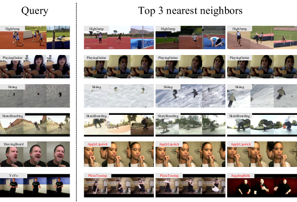
(a)

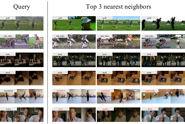
(b)

Figure 6: Downstream video retrieval results. (a) Six examples of UCF101 dataset. (b) Six examples of HMDB51 dataset. Within each six examples, top four rows are correct retrievals and the last two rows are incorrect.

(a)

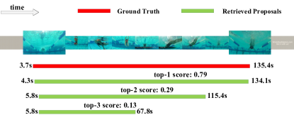
(b)

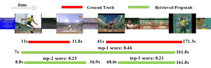
(c)

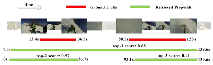
(d)

Figure 7: Downstream action localization results. We show our top-3 proposals and most of them align closely with the ground truth action instance.

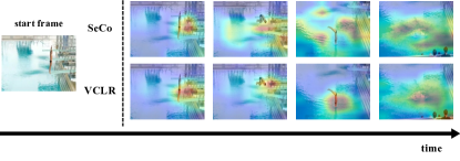
(a)

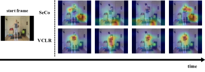
(b)

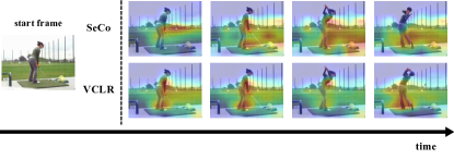
(c)

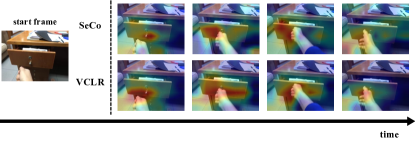
(d)

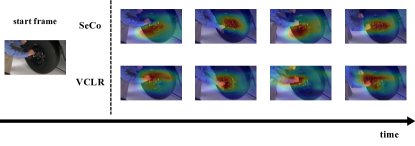
(e)

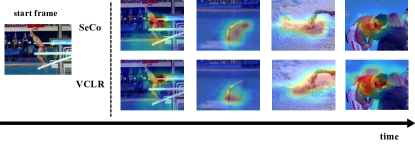
(f)

Figure 8: More feature visualizations based on Grad-CAM. (a) to (f) are examples from Kinetics400, UCF101, HMDB51, SthSthV2, ActivityNet, and unseen video respectively.

References

- [1] Jean-Baptiste Alayrac, Adrià Recasens, Rosalia Schneider, Relja Arandjelović, Jason Ramapuram, Jeffrey De Fauw, Lucas Smaira, Sander Dieleman, and Andrew Zisserman. Self-supervised multimodal versatile networks. In NeurIPS, 2020.
- [2] Humam Alwassel, Dhruv Mahajan, Bruno Korbar, Lorenzo Torresani, Bernard Ghanem, and Du Tran. Self-supervised learning by cross-modal audio-video clustering. In NeurIPS, 2020.
- [3] Nadine Behrmann, Jurgen Gall, and Mehdi Noroozi. Unsupervised video representation learning by bidirectional feature prediction. In WACV, 2021.
- [4] Sagie Benaim, Ariel Ephrat, Oran Lang, Inbar Mosseri, William T. Freeman, Michael Rubinstein, Michal Irani, and Tali Dekel. SpeedNet: Learning the Speediness in Videos. In CVPR, 2020.
- [5] Uta Buchler, Biagio Brattoli, and Bjorn Ommer. Improving Spatiotemporal Self-Supervision by Deep Reinforcement Learning. In ECCV, 2018.
- [6] Fabian Caba Heilbron, Victor Escorcia, Bernard Ghanem, and Juan Carlos Niebles. ActivityNet: A Large-Scale Video Benchmark for Human Activity Understanding. In CVPR, 2015.
- [7] Mathilde Caron, Ishan Misra, Julien Mairal, Priya Goyal, Piotr Bojanowski, and Armand Joulin. Unsupervised Learning of Visual Features by Contrasting Cluster Assignments. arXiv preprint arXiv:2006.09882, 2020.
- [8] Peihao Chen, Deng Huang, Dongliang He, Xiang Long, Runhao Zeng, Shilei Wen, Mingkui Tan, and Chuang Gan. Rspnet: Relative speed perception for unsupervised video representation learning. In AAAI, 2021.
- [9] Ting Chen, Simon Kornblith, Mohammad Norouzi, and Geoffrey Hinton. A Simple Framework for Contrastive Learning of Visual Representations. In ICML. 2020.
- [10] Ting Chen, Simon Kornblith, Kevin Swersky, Mohammad Norouzi, and Geoffrey Hinton. Big Self-Supervised Models are Strong Semi-Supervised Learners. arXiv preprint arXiv:2006.10029, 2020.
- [11] Xinlei Chen, Haoqi Fan, Ross Girshick, and Kaiming He. Improved Baselines with Momentum Contrastive Learning. arXiv preprint arXiv:2003.04297, 2020.
- [12] Chen Sun and Fabien Baradel and Kevin Murphy, Cordelia Schmid. Learning Video Representations using Contrastive Bidirectional Transformer. arXiv preprint arXiv:1906.05743, 2019.
- [13] MMAction2 Contributors. Openmmlab’s next generation video understanding toolbox and benchmark. https://github.com/open-mmlab/mmaction2, 2020.
- [14] Jacob Devlin, Ming-Wei Chang, Kenton Lee, and Kristina Toutanova. BERT: Pre-training of Deep Bidirectional Transformers for Language Understanding. arXiv preprint arXiv:1810.04805, 2018.
- [15] Ali Diba, Vivek Sharma, Luc Van Gool, and Rainer Stiefelhagen. DynamoNet: Dynamic Action and Motion Network. In ICCV, 2019.
- [16] Ali Diba, Vivek Sharma, and Luc Van Gool. Deep Temporal Linear Encoding Networks. In CVPR, 2017.
- [17] Debidatta Dwibedi, Yusuf Aytar, Jonathan Tompson, Pierre Sermanet, and Andrew Zisserman. Temporal Cycle-Consistency Learning. In CVPR, 2019.
- [18] Christoph Feichtenhofer, Haoqi Fan, Bo Xiong, Ross Girshick, and Kaiming He. A large-scale study on unsupervised spatiotemporal representation learning. In CVPR, 2021.
- [19] Basura Fernando, Hakan Bilen, Efstratios Gavves, and Stephen Gould. Self-Supervised Video Representation Learning with Odd-One-Out Networks. In CVPR, 2017.
- [20] Rohit Girdhar, Deva Ramanan, Abhinav Gupta, Josef Sivic, and Bryan Russell. ActionVLAD: Learning Spatio-Temporal Aggregation for Action Classification. In CVPR, 2017.
- [21] Daniel Gordon, Kiana Ehsani, Dieter Fox, and Ali Farhadi. Watching the World Go By: Representation Learning from Unlabeled Videos. arXiv preprint arXiv:2003.07990, 2020.
- [22] Raghav Goyal, Samira Ebrahimi Kahou, Vincent Michalski, Joanna Materzynska, Susanne Westphal, Heuna Kim, Valentin Haenel, Ingo Fruend, Peter Yianilos, Moritz Mueller-Freitag, et al. The” Something Something” Video Database for Learning and Evaluating Visual Common Sense. In ICCV, 2017.
- [23] Jean-Bastien Grill, Florian Strub, Florent Altché, Corentin Tallec, Pierre H. Richemond, Elena Buchatskaya, Carl Doersch, Bernardo Avila Pires, Zhaohan Daniel Guo, Mohammad Gheshlaghi Azar, Bilal Piot, Koray Kavukcuoglu, Rémi Munos, and Michal Valko. Bootstrap Your Own Latent: A New Approach to Self-Supervised Learning. arXiv preprint arXiv:2006.07733, 2020.
- [24] Xudong Guo, Xun Guo, and Yan Lu. Ssan: Separable self-attention network for video representation learning. In CVPR, 2021.
- [25] Tengda Han, Weidi Xie, and Andrew Zisserman. Video Representation Learning by Dense Predictive Coding. In ICCVW, 2019.
- [26] Tengda Han, Weidi Xie, and Andrew Zisserman. Memory-augmented Dense Predictive Coding for Video Representation Learning. In ECCV, 2020.
- [27] Tengda Han, Weidi Xie, and Andrew Zisserman. Self-supervised Co-training for Video Representation Learning. In NeurIPS, 2020.
- [28] Kensho Hara, Hirokatsu Kataoka, and Yutaka Satoh. Can Spatiotemporal 3D CNNs Retrace the History of 2D CNNs and ImageNet? In CVPR, 2018.
- [29] Kaiming He, Haoqi Fan, Yuxin Wu, Saining Xie, and Ross Girshick. Momentum Contrast for Unsupervised Visual Representation Learning. In CVPR. 2020.
- [30] Kaiming He, Xiangyu Zhang, Shaoqing Ren, and Jian Sun. Deep Residual Learning for Image Recognition. In CVPR. 2016.
- [31] Lianghua Huang, Yu Liu, Bin Wang, Pan Pan, Yinghui Xu, and Rong Jin. Self-supervised video representation learning by context and motion decoupling. In CVPR, 2021.
- [32] Allan Jabri, Andrew Owens, and Alexei A Efros. Space-Time Correspondence as a Contrastive Random Walk. NeurIPS, 2020.
- [33] Simon Jenni, Givi Meishvili, and Paolo Favaro. Video Representation Learning by Recognizing Temporal Transformations. In ECCV, 2020.
- [34] Longlong Jing, Xiaodong Yang, Jingen Liu, and Yingli Tian. Self-supervised Spatiotemporal Feature Learning via Video Rotation Prediction. arXiv preprint arXiv:1811.11387, 2018.
- [35] Will Kay, Joao Carreira, Karen Simonyan, Brian Zhang, Chloe Hillier, Sudheendra Vijayanarasimhan, Fabio Viola, Tim Green, Trevor Back, Paul Natsev, Mustafa Suleyman, and Andrew Zisserman. The Kinetics Human Action Video Dataset. arXiv preprint arXiv:1705.06950, 2017.
- [36] Dahun Kim, Donghyeon Cho, and In So Kweon. Self-Supervised Video Representation Learning with Space-Time Cubic Puzzles. In AAAI, 2019.
- [37] Bruno Korbar, Du Tran, and Lorenzo Torresani. Cooperative learning of audio and video models from self-supervised synchronization. In NeurIPS, 2018.
- [38] Hildegard Kuehne, Hueihan Jhuang, Estíbaliz Garrote, Tomaso Poggio, and Thomas Serre. HMDB: A Large Video Database for Human Motion Recognition. In ICCV, 2011.
- [39] Zhenzhong Lan, Yi Zhu, Alexander G Hauptmann, and Shawn Newsam. Deep local video feature for action recognition. In CVPRW, 2017.
- [40] Hsin-Ying Lee, Jia-Bin Huang, Maneesh Singh, and Ming-Hsuan Yang. Unsupervised Representation Learning by Sorting Sequences. In ICCV, 2017.
- [41] Xinyu Li, Chunhui Liu, Bing Shuai, Yi Zhu, Hao Chen, and Joseph Tighe. Nuta: Non-uniform temporal aggregation for action recognition. arXiv preprint arXiv:2012.08041, 2020.
- [42] Xinyu Li, Yanyi Zhang, Chunhui Liu, Bing Shuai, Yi Zhu, Biagio Brattoli, Hao Chen, Ivan Marsic, and Joseph Tighe. VidTr: Video Transformer Without Convolutions. In ICCV, 2021.
- [43] Ji Lin, Chuang Gan, and Song Han. TSM: Temporal Shift Module for Efficient Video Understanding. In ICCV, 2019.
- [44] Tianwei Lin, Xiao Liu, Xin Li, Errui Ding, and Shilei Wen. BMN: Boundary-Matching Network for Temporal Action Proposal Generation. In ICCV, 2019.
- [45] Dezhao Luo, Chang Liu, Yu Zhou, Dongbao Yang, Can Ma, Qixiang Ye, and Weiping Wang. Video Cloze Procedure for Self-Supervised Spatio-Temporal Learning. In AAAI, 2020.
- [46] Zelun Luo, Boya Peng, De-An Huang, Alexandre Alahi, and Li Fei-Fei. Unsupervised Learning of Long-Term Motion Dynamics for Videos. In CVPR, 2017.
- [47] Antoine Miech, Jean-Baptiste Alayrac, Lucas Smaira, Ivan Laptev, Josef Sivic, and Andrew Zisserman. End-to-end learning of visual representations from uncurated instructional videos. In CVPR, 2020.
- [48] Ishan Misra, C Lawrence Zitnick, and Martial Hebert. Shuffle and Learn: Unsupervised Learning using Temporal Order Verification. In ECCV, 2016.
- [49] Tian Pan, Yibing Song, Tianyu Yang, Wenhao Jiang, and Wei Liu. Videomoco: Contrastive video representation learning with temporally adversarial examples. In CVPR, 2021.
- [50] Mandela Patrick, Yuki M Asano, Polina Kuznetsova, Ruth Fong, João F Henriques, Geoffrey Zweig, and Andrea Vedaldi. Multi-modal self-supervision from generalized data transformations. arXiv preprint arXiv:2003.04298, 2020.
- [51] AJ Piergiovanni, Anelia Angelova, and Michael S Ryoo. Evolving losses for unsupervised video representation learning. In CVPR, 2020.
- [52] Rui Qian, Tianjian Meng, Boqing Gong, Ming-Hsuan Yang, Huisheng Wang, Serge Belongie, and Yin Cui. Spatiotemporal Contrastive Video Representation Learning. In CVPR, 2021.
- [53] Ramprasaath R Selvaraju, Michael Cogswell, Abhishek Das, Ramakrishna Vedantam, Devi Parikh, and Dhruv Batra. Grad-cam: Visual explanations from deep networks via gradient-based localization. In ICCV, 2017.
- [54] Khurram Soomro, Amir Roshan Zamir, and Mubarak Shah. UCF101: A Dataset of 101 Human Actions Classes From Videos in The Wild. arXiv preprint arXiv:1212.0402, 2012.
- [55] Tian, Yonglong and Krishnan, Dilip and Isola, Phillip. Contrastive Multiview Coding. arXiv preprint arXiv:1906.05849, 2019.
- [56] Aaron van den Oord, Yazhe Li, and Oriol Vinyals. Representation Learning with Contrastive Predictive Coding. arXiv preprint arXiv:1807.03748, 2018.
- [57] Carl Vondrick, Hamed Pirsiavash, and Antonio Torralba. Unsupervised Learning of Video Representations using LSTMs. In ICML, 2015.
- [58] Carl Vondrick, Hamed Pirsiavash, and Antonio Torralba. Anticipating Visual Representations from Unlabeled Video. In CVPR, 2016.
- [59] Guangting Wang, Yizhou Zhou, Chong Luo, Wenxuan Xie, Wenjun Zeng, and Zhiwei Xiong. Unsupervised visual representation learning by tracking patches in video. In CVPR, 2021.
- [60] Jinpeng Wang, Yuting Gao, Ke Li, Xinyang Jiang, Xiaowei Guo, Rongrong Ji, and Xing Sun. Enhancing unsupervised video representation learning by decoupling the scene and the motion. In AAAI, 2021.
- [61] Jinpeng Wang, Yuting Gao, Ke Li, Yiqi Lin, Andy J Ma, Hao Cheng, Pai Peng, Feiyue Huang, Rongrong Ji, and Xing Sun. Removing the background by adding the background: Towards background robust self-supervised video representation learning. In CVPR, 2021.
- [62] Jiangliu Wang, Jianbo Jiao, Linchao Bao, Shengfeng He, Yunhui Liu, and Wei Liu. Self-Supervised Spatio-Temporal Representation Learning for Videos by Predicting Motion and Appearance Statistics. In CVPR, 2019.
- [63] Jiangliu Wang, Jianbo Jiao, and Yunhui Liu. Self-Supervised Video Representation Learning by Pace Prediction. In ECCV, 2020.
- [64] Limin Wang, Yuanjun Xiong, Zhe Wang, Yu Qiao, Dahua Lin, Xiaoou Tang, and Luc Van Gool. Temporal Segment Networks: Towards Good Practices for Deep Action Recognition. In ECCV, 2016.
- [65] Xiaolong Wang, Ross Girshick, Abhinav Gupta, and Kaiming He. Non-Local Neural Networks. In CVPR, 2018.
- [66] Xiaolong Wang, Allan Jabri, and Alexei A. Efros. Learning Correspondence from the Cycle-Consistency of Time. In CVPR, 2019.
- [67] Donglai Wei, Joseph J. Lim, Andrew Zisserman, and William T. Freeman. Learning and Using the Arrow of Time. In CVPR, 2018.
- [68] Chao-Yuan Wu, Christoph Feichtenhofer, Haoqi Fan, Kaiming He, Philipp Krahenbuhl, and Ross Girshick. Long-Term Feature Banks for Detailed Video Understanding. In CVPR, 2019.
- [69] Zhirong Wu, Yuanjun Xiong, Stella Yu, and Dahua Lin. Unsupervised Feature Learning via Non-Parametric Instance-level Discrimination. In CVPR. 2018.
- [70] Saining Xie, Chen Sun, Jonathan Huang, Zhuowen Tu, and Kevin Murphy. Rethinking Spatiotemporal Feature Learning: Speed-Accuracy Trade-offs in Video Classification. In ECCV, 2018.
- [71] Dejing Xu, Jun Xiao, Zhou Zhao, Jian Shao, Di Xie, and Yueting Zhuang. Self-Supervised Spatiotemporal Learning via Video Clip Order Prediction. In CVPR, 2019.
- [72] Ceyuan Yang, Yinghao Xu, Bo Dai, and Bolei Zhou. Video Representation Learning with Visual Tempo Consistency. 2020.
- [73] Ting Yao, Yiheng Zhang, Zhaofan Qiu, Yingwei Pan, and Tao Mei. SeCo: Exploring Sequence Supervision for Unsupervised Representation Learning. In AAAI, 2021.
- [74] Yuan Yao, Chang Liu, Dezhao Luo, Yu Zhou, and Qixiang Ye. Video Playback Rate Perception for Self-supervisedSpatio-Temporal Representation Learning. In CVPR, 2020.
- [75] Shiwen Zhang, Sheng Guo, Weilin Huang, Matthew R. Scott, and Limin Wang. V4D:4D Convolutional Neural Networks for Video-level Representation Learning. In ICLR, 2020.
- [76] Hang Zhao, Zhicheng Yan, Lorenzo Torresani, and Antonio Torralba. HACS: Human Action Clips and Segments Dataset for Recognition and Temporal Localization. arXiv preprint arXiv:1712.09374, 2019.
- [77] Yi Zhu, Zhenzhong Lan, Shawn Newsam, and Alexander G Hauptmann. Hidden Two-Stream Convolutional Networks for Action Recognition. In ACCV, 2018.
- [78] Yi Zhu, Xinyu Li, Chunhui Liu, Mohammadreza Zolfaghari, Yuanjun Xiong, Chongruo Wu, Zhi Zhang, Joseph Tighe, R Manmatha, and Mu Li. A comprehensive study of deep video action recognition. arXiv preprint arXiv:2012.06567, 2020.
- [79] Chengxu Zhuang, Tianwei She, Alex Andonian, Max Sobol Mark, and Daniel Yamins. Unsupervised Learning From Video With Deep Neural Embeddings. In CVPR, 2020.