Two-particle scattering from finite-volume quantization conditions using the plane wave basis

Abstract

We propose an alternative approach to Lüscher’s formula for extracting two-body scattering phase shifts from finite volume spectra with no reliance on the partial wave expansion. We use an effective-field-theory-based Hamiltonian method in the plane wave basis and decompose the corresponding matrix elements of operators into irreducible representations of the relevant point groups. The proposed approach allows one to benefit from the knowledge of the long-range interaction and avoids complications from partial wave mixing in a finite volume. We consider spin-singlet channels in the two-nucleon system and pion-pion scattering in the $\rho$-meson channel in the rest and moving frames to illustrate the method for non-relativistic and relativistic systems, respectively. For the two-nucleon system, the long-range interaction due to the one-pion exchange is found to make the single-channel Lüscher formula unreliable at the physical pion mass. For S-wave dominated states, the single-channel Lüscher method suffers from significant finite-volume artifacts for a $L=3$ fm box, but it works well for boxes with $L>5$ fm. However, for P-wave dominated states, significant partial wave mixing effects prevent the application of the single-channel Lüscher formula regardless of the box size (except for the near-threshold region). Using a toy model to generate synthetic data for finite-volume energies, we show that our effective-field-theory-based approach in the plane wave basis is capable of a reliable extraction of the phase shifts. For pion-pion scattering, we employ a phenomenological model to fit lattice QCD results at the physical pion mass. The extracted P-wave phase shifts are found to be in a good agreement with the experimental results.

1 Introduction

Three decades ago, Lüscher proposed a model-independent approach for extracting two-particle elastic scattering phase shifts from energy levels in a finite box with periodic boundary conditions Luscher:1985dn ; Luscher:1986pf ; Luscher:1990ux . This seminal work opened the way for investigating hadronic scattering observables using lattice QCD simulations. The Lüscher formula has been generalized to moving systems in finite boxes Rummukainen:1995vs ; Kim:2005gf ; Gockeler:2012yj , higher partial waves Luu:2011ep , particles with different masses Fu:2011xz ; Leskovec:2012gb , particles with nonzero spins Briceno:2014oea , multichannel scattering Lage:2009zv ; He:2005ey ; Hansen:2012tf ; Doring:2012eu and to cases with asymmetric boxes Feng:2004ua , see also Briceno:2017max ; Mai:2021lwb for review articles.

The Lüscher method assumes that the box size $L$ is much larger than the interaction range $R$, such that exponentially suppressed corrections $\sim e^{-L/R}$ are negligible. In currently feasible lattice simulations, the box size can usually not be chosen very large given the available computational resources. On the other hand, in certain cases such as e.g. the two-nucleon system, the long-range interaction is known and appears to play a very prominent role. Another example of a system featuring long-range dynamics is the $\bar{D}^{*}D/\bar{D}D^{*}$ system, in which the one-pion exchange (OPE) potential plays an important role for the formation of exotic hadrons $X(3872)$ and $Z_{c}(3900)$ Chen:2016qju ; Guo:2017jvc ; Brambilla:2019esw . The accidental mass relation $m_{\bar{D}^{*}}\approx m_{\bar{D}}+M_{\pi}$ makes the exchanged pion in the OPE potential almost on-shell, which results in the interaction range much larger than $1/M_{\pi}$. In such situations, taking into account the long-range dynamics may allow one to reduce the cost of lattice QCD simulations by considering smaller volumes. It, however, requires the finite-volume Lüscher quantization conditions to be generalized by taking into account exponentially suppressed effects due to the long-range interaction.

In single-channel cases, each energy level in a finite volume (FV) can be related to the scattering phase shift at this energy using interaction-independent Lüscher’s formula. On the other hand, one has to deal with coupled-channel effects when taking into account inelastic channels or partial wave mixing. In the multichannel case, Lüscher’s formula becomes a determinant equation $\det[f(T,E)]=0$, which relates the $T$-matrix and the FV energy levels. Though this result is still model-independent, there is no one-to-one correspondences between phase shifts and FV energy levels. It does not allow one to extract the full $T$-matrix, i.e. phase shifts for every channel and the corresponding mixing angles. In practice, the $T$-matrix can be parameterized within a particular theoretical framework, and several FV energies can be used as input to determine the parameters in the $T$-matrix. This may, however, introduce some model dependence. Another complication is related to rotational symmetry breaking in finite boxes, which results in the energy levels generally receiving contributions from multiple partial waves.

In the literature, much effort has been devoted to cure or estimate the two drawbacks of the Lüscher formula, namely exponentially suppressed corrections and mixing effects in multichannel scattering. In refs. Bedaque:2006yi ; Sato:2007ms , the authors estimated exponentially suppressed corrections for $\pi\pi$ and NN scatterings in the FV. It was shown that for realistic pion masses, simulations in a box of the size $L>5$ fm would result in exponential corrections to the phase shifts less than one degree. In ref. Jansen:2015lha , finite volume corrections to the $X(3872)$ were analyzed in an effective field theory (EFT) with perturbative pions. It was shown that FV effects are significant for box lengths as large as $20$ fm. Unitarized chiral perturbation theory in a finite volume was employed in refs. Doring:2011vk ; Doring:2012eu ; Guo:2016zep ; Guo:2018tjx , in which some exponentially suppressed effects were included by adopting a fully relativistic propagator. Such exponentially suppressed differences with the Lüscher formula for $\pi\pi$ scattering were calculated explicitly in refs. Albaladejo:2012jr ; Chen:2012rp . In order to deal with coupled-channel effects in a FV, an effective Hamiltonian approach was developed in refs. Hall:2013qba ; Wu:2014vma ; Liu:2015ktc ; Li:2021mob . Within different approaches, partial wave mixing effects were estimated in refs. Luu:2011ep ; Doring:2012eu ; Morningstar:2017spu ; Li:2019qvh . The sensitivity to the second lowest partial wave in Lüscher’s quantization conditions was discussed in ref. Lee:2021kfn .

Starting from Lüscher’s seminal work, FV effects were usually investigated using the partial wave expansion technique. In the infinite volume, partial wave expansion allows one to simplify the scattering problem thanks to the rotational symmetry. However, in the finite volume, continuous rotational symmetry is broken and the angular momentum is no longer a good quantum number. To some extent, introducing the partial wave expansion in a finite volume complicates the problem. For small boxes and/or systems with coupled channels as well as in the presence of long-range interactions, the above mentioned drawbacks of the Lüscher approach get amplified. A natural alternative method is to employ vectors of discrete momenta. In refs. Luu:2011ep ; Li:2019qvh , the authors used the discrete momentum basis to investigate partial wave mixing effects. Recently, a Fourier basis $\{\cos(2\pi n_{i}r_{i}/L),\sin(2\pi n_{i}r_{i}/L)\}$ in coordinate space was adopted to diagonalize the Hamiltonian in FV Lee:2020fbo .

In this work, we employ a similar approach as that of ref. Lee:2020fbo but in momentum space. We consider the Lippmann-Schwinger equation (LSE) in the non-relativistic case or a reduced Bethe-Salpeter equation (BSE) in the relativistic case using the plane wave basis with discrete momenta. Next, we reduce the matrix LSE and BSE into the irreducible representations (irreps) of the cubic group. With the reduced matrix equation, we compute the energy levels in the FV corresponding to specific irreps. In such a framework, effects from mixing with higher partial waves are embedded naturally. We also extend this approach to systems with nonvanishing total momentum. We consider NN and $\pi\pi$ scattering as examples of the non-relativistic and relativistic systems, respectively, to illustrate the calculations and compare our results with those obtained using the single-channel Lüscher approach. In the case of the NN system, we also study the role played by the long-range interaction due to the one-pion exchange.

This work is organized as follows. In section 2, we review the discretization conditions of three-momenta and discuss the relevant symmetry groups for two particles in a cubic box with periodic boundary conditions. In section 3, we construct the representation spaces of the corresponding point groups with the plane wave basis and perform their reduction into irreps using the projection operator technique. In section 4, we introduce a general approach to obtain the FV energy levels and to fit lattice QCD energy spectra in the FV. Next, in section 5, we consider spin-singlet NN scattering as an explicit example of a non-relativistic system to demonstrate our method. In this section, we also discuss in detail partial wave mixing effects in the FV. In section 6, we consider $\pi\pi$ scattering in the $\rho$-meson channel as an example of a relativistic system. Using a phenomenological model to parameterize the $\pi\pi$ scattering amplitude, we calculate the FV energy levels and fit the parameters of the model to the lattice QCD spectra. Finally, in section 7, we summarize the main results of our study and discuss possible generalizations. Some basic information about the point groups used in this work and Lüscher’s quantization conditions is given in appendices A and B.

2 Two particles in a finite volume

Discretization of three-momenta of two particles in a cubic box with periodic boundary conditions is considered e.g. in refs. Rummukainen:1995vs ; Leskovec:2012gb . In the following, we briefly review the relevant findings for the sake of completeness. Throughout this paper, we focus on systems of two spinless particles of the same mass. It is straightforward to generalize our results to particles with arbitrary spin and different masses.

2.1 Non-interacting case

In the box frame (BF), the momenta $\bm{p}_{1}$ and $\bm{p}_{2}$ of two non-interacting particles are discrete,

$$E=\sqrt{\bm{p}_{1}^{2}+m_{1}^{2}}+\sqrt{\bm{p}_{2}^{2}+m_{2}^{2}},$$ (1)

$$\bm{p}_{1}+\bm{p}_{2}=\bm{P},\quad\bm{p}_{1}=\frac{2\pi}{L}\bm{n},\quad\bm{P}=\frac{2\pi}{L}\bm{d},\qquad\bm{n},\bm{d}\in{Z}^{3},$$ (2)

where $\bm{P}$ and $E$ are the total momentum and energy of the two-particle system, respectively. For the non-interacting case, each particle is on-shell with $E_{i}=\sqrt{\bm{p}_{i}^{2}+m_{i}^{2}}$. In the center-of-mass frame (CMF), the related momenta and energies read

$$\bm{P}^{*}=0,\quad\bm{p}^{*}\equiv\frac{1}{2}(\bm{p}_{1}^{*}-\bm{p}_{2}^{*})=\bm{p}_{1}^{*}=-\bm{p}_{2}^{*},\quad E^{*2}=E^{2}-\bm{P}^{2},~{}$$ (3)

where the quantities in the CMF are labeled by superscript “$*$”. In eq. (3), the on-shell relation of each particle is not used. Thus, eq. (3) is also valid for interacting systems. For non-interacting systems, the momentum and energy in the CMF are related to those in the BF by the Lorentz transformation

$$\bm{p}_{1}^{*} = \left[(\gamma-1)\frac{\bm{P}\cdot\bm{p}_{1}}{\bm{P}^{2}}-\frac{E_{1}}{E^{*}}\right]\bm{P}+\bm{p}_{1},$$ (4)

$$E_{1}^{*} = \frac{EE_{1}-\bm{P}\cdot\bm{p}_{1}}{E^{*}},$$ (5)

where $\gamma=\frac{E}{E^{*}}$ is the Lorentz factor. Equations (4) and (5) can be combined and simplified to

$$\bm{p}_{1}^{*}=\gamma^{-1}\left(\bm{p}_{1\parallel}-\frac{1}{2}A\bm{P}\right)+\bm{p}_{1\perp},$$ (6)

where

$$A\equiv 1+\frac{m_{1}^{2}-m_{2}^{2}}{E^{*2}}.$$ (7)

For a given vector $\bm{u}$, $\bm{u}_{\parallel}$ and $\bm{u}_{\perp}$ are defined via $\bm{u}_{\parallel}=\frac{(\bm{u}\cdot\bm{P})\bm{P}}{\bm{P}^{2}}$ and $\bm{u}_{\perp}=\bm{u}-\bm{u}_{\parallel}$.

In this paper we are interested in systems of two particles with equal masses (and thus $A=1$). With eqs. (2) and (6), one obtains the discretization relations in the CMF

$$\bm{p}^{*}=\bm{n}^{*}\frac{2\pi}{L},\quad\bm{n}^{*}\in P_{d},$$

$$P_{d}=\{\gamma^{-1}(\bm{n}_{\parallel}-\frac{1}{2}\bm{d})+\bm{n}_{\perp}\},\quad\bm{n}\in{Z}^{3}.$$ (8)

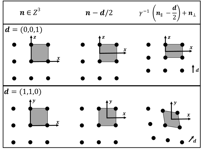
Figure 1: Meshes of the set of discrete momenta for a two-particle system with equal masses in the BF (left column) and CMF (right column). The second and third meshes in each row illustrate the shift of the origin by $\bm{d}/2$ and the deformation in the direction of $\bm{d}$ to obtain the mesh in the CMF.

In figure 1, we show a set of discrete momenta with the corresponding meshes in different frames. The first mesh in each row corresponds to the momenta in the BF. The second and third ones illustrate the steps needed to obtain the momenta in the CMF according to eq. (8), namely the shift of the origin by $\bm{d}/2$ and the deformation in the direction of $\bm{d}$. In figure 1, we take $\bm{d}=(0,0,1)$ and $\bm{d}=(1,1,0)$ as examples. The meshes show the symmetries of the system in the FV. In the infinite volume, the momenta are continuous and satisfy the rotational symmetry described by the $SO(3)$ group. Considering the conservation of space inversion, the symmetric group becomes $O(3)=SO(3)\otimes\{E,I\}$, where $E$ and $I$ are the identity and the space inversion elements, respectively. In the BF corresponding to $\bm{d}=(0,0,0)$, the symmetry group is the cubic $O_{h}=O\otimes\{E,I\}$ one, which is a subgroup of the $O(3)$ group. When the two-particle system is moving in the box, the $O_{h}$ symmetry is broken by shifting the origin and a deformation in the direction of $\bm{d}$. The symmetric point groups corresponding to different values of $\bm{d}$ are presented in table 1. In this work we are only interested in the $d^{2}=0,1,2,3,4$ cases and, therefore, consider only the $O_{h}$, $D_{4h}$, $D_{2h}$ and $D_{3d}$ groups and the corresponding subgroups $O$, $D_{4}$, $D_{2}$ and $D_{3}$ containing only proper rotations. It should be noticed that the symmetric groups considered here are only applicable to the case of two particles with equal masses. For particles with different masses ($A\neq 1$), the origin of the coordinate system in figure 1 is not in the center of its adjacent points anymore after shifting by ${1\over 2}A\bm{d}$, and the system is not invariant with respect to space inversions Leskovec:2012gb . In appendix A, we list the group elements, conjugacy classes, and character tables for the relevant point groups.

$\bm{d}$	point group	$n_{G}$	representation space
$(0,0,0)$	$O_{h}$	48	$\{n_{1},n_{2},n_{3}\}$
$(0,0,a)$	$D_{4h}$	16	$\{n_{1},n_{2};n_{3}\}$
$(a,a,0)$	$D_{2h}$	8	$\{n_{1},n_{2};n_{3}\}$
$(a,a,a)$	$D_{3d}$	12	$\{n_{1},n_{2},n_{3}\}$

Table 1: The point groups, their orders $n_{G}$, and representation spaces of the two-particle systems in finite volume as defined in eqs. (16) and (17).

In the literature, two conventions to denote irreps of $D_{4h}$, $D_{2h}$ and $D_{3d}$ are used. For example, the $D_{4h}$ group can be formed either as $D_{4h}=D_{4}\otimes\{E,I\}$ or as $D_{4h}=C_{4v}\otimes\{E,I\}$. The elements of $D_{4}$ are all proper rotations. The $C_{4v}$ group contains two improper rotations and is the symmetry group for systems with particles of unequal masses. In the first convention, the irreps of $D_{4h}$ are denoted by the irreps of the $D_{4}$ group with parity Rummukainen:1995vs ; Briceno:2013lba . In the second convention, the irreps of $D_{4h}$ are denoted by the irreps of the $C_{4v}$ group with parity Gockeler:2012yj ; Morningstar:2013bda . We list the irreps of the two conventions and their corresponding relations in table 2. In this work, we adopt the first convention.

Point group	Two conventions		irreps with even parity					irreps with odd parity
$O_{h}$		$O\otimes\{I,E\}$	$A_{1}^{+}$	$A_{2}^{+}$	$E^{+}$	$T_{1}^{+}$	$T_{2}^{+}$	$A_{1}^{-}$	$A_{2}^{-}$	$E^{-}$	$T_{1}^{-}$	$T_{2}^{-}$
$D_{4h}$	I	$D_{4}\otimes\{I,E\}$	$A_{1}^{+}$	$A_{2}^{+}$	$B_{1}^{+}$	$B_{2}^{+}$	$E^{+}$	$A_{1}^{-}$	$A_{2}^{-}$	$B_{1}^{-}$	$B_{2}^{-}$	$E^{-}$
	II	$C_{4v}\otimes\{I,E\}$	$A_{1}^{+}$	$A_{2}^{+}$	$B_{1}^{+}$	$B_{2}^{+}$	$E^{+}$	$A_{2}^{-}$	$A_{1}^{-}$	$B_{2}^{-}$	$B_{1}^{-}$	$E^{-}$
$D_{2h}$	I	$D_{2}\otimes\{I,E\}$	$A_{1}^{+}$	$B_{1}^{+}$	$B_{2}^{+}$	$B_{3}^{+}$		$A_{1}^{-}$	$B_{1}^{-}$	$B_{2}^{-}$	$B_{3}^{-}$
	II	$C_{2v}\otimes\{I,E\}$	$A_{1}^{+}$	$A_{2}^{+}$	$B_{1}^{+}$	$B_{2}^{+}$		$A_{2}^{-}$	$A_{1}^{-}$	$B_{2}^{-}$	$B_{1}^{-}$
$D_{3d}$	I	$D_{3}\otimes\{I,E\}$	$A_{1}^{+}$	$A_{2}^{+}$	$E^{+}$			$A_{1}^{-}$	$A_{2}^{-}$	$E^{-}$
	II	$C_{3v}\otimes\{I,E\}$	$A_{1}^{+}$	$A_{2}^{+}$	$E^{+}$			$A_{2}^{-}$	$A_{1}^{-}$	$E^{+}$

Table 2: Irreps of the relevant point groups using the two conventions as discussed in the text and their corresponding relations. The convention I is adopted in ref. Rummukainen:1995vs ; Briceno:2013lba and in this paper. The convention II is employed in refs. Gockeler:2012yj ; Morningstar:2013bda .

For non-relativistic systems, the above discussion can be simplified since the Lorentz factor becomes $\gamma=1$ and the Lorentz transformation reduces to the Galilean one. Thus, the second step in figure 1 is unnecessary. One consequence is that the meshes for non-relativistic systems might be more symmetric than the ones with the same $\bm{d}$ in a relativistic theory. For example, in a non-relativistic theory, the mesh for the $\bm{d}=(0,0,2)$ system is the same as that of the $\bm{d}=(0,0,0)$ system. The shift of origin by ${\bm{d}/2}=(0,0,1)$ in figure 1 makes no difference for momentum discretization. Thus, the discrete symmetry group of a non-relativistic system with $\bm{d}=(0,0,2)$ is $O_{h}$. However, the relativistic system with the same $\bm{d}$ only possesses the $D_{4h}$ symmetry. In this work, for calculational convenience, we adopt an unified approach for both non-relativistic and relativistic systems. E.g., for a given system with $\bm{d}=(0,0,2)$, we classify the energy levels according to the irreps of $D_{4h}$. Thus, for non-relativistic systems, we will end up with several degenerate states in different irreps reflecting the additional degeneracy of the more symmetric group $O_{h}$.

2.2 Interacting case

To compute FV energy spectra in the interacting case, we need to perform boost transformations for loop momenta with particles being off shell, i.e. $E_{i}^{(*)2}\neq m_{i}^{2}+\bm{p}_{i}^{(*)2}$. In the literature, different schemes have been proposed to define the quantization conditions for the cases with $\bm{P}\neq 0$. The one of ref. Doring:2012eu starts with the prescription

$$E_{1,2}^{*}=\frac{E^{*2}+m_{1,2}^{2}-m_{2,1}^{2}}{2E^{*}}\,,$$ (9)

which is the same as in the non-interacting case and ensures that $E_{1}^{*}+E_{2}^{*}=E^{*}$, and $E_{1}^{*}=E_{2}^{*}={E^{*}\over 2}$ for $m_{1}=m_{2}$. By substituting eq. (9) into eqs. (4) and  (5), one obtains the same quantization conditions as those in eqs. (6) and (8).

Recently, an alternative scheme was proposed in ref. Li:2021mob . Their relation of $\bm{p}_{1}^{*}$ with $\bm{p}_{1}$ reads

$$\bm{p}_{1}^{*}=\left[(\gamma-1)\frac{\bm{P}\cdot\bm{p}_{1}}{\bm{P}^{2}}-\frac{\omega_{1}}{\sqrt{(\omega_{1}+\omega_{2})^{2}-P^{2}}}\right]\bm{P}+\bm{p}_{1},$$ (10)

where $\omega_{i}=\sqrt{m_{1}^{2}+\bm{p}_{i}^{2}}$. The Lorentz factor $\gamma$ is defined as

$$\gamma=\frac{\omega_{1}+\omega_{2}}{\sqrt{(\omega_{1}+\omega_{2})^{2}-\bm{P}^{2}}}\,.$$ (11)

In the first scheme, the Lorentz factor $\gamma$ is defined rigorously, and it only depends on the total energies of the two-particle system in the BF and CMF. In the second scheme, the Lorentz factor is taken as an approximation using the expression for the non-interacting case. Such an approximation makes the transformation independent of the energy, which simplifies the determination of poles of the $T$-matrix. It was argued that the difference between the two schemes is exponentially suppressed Li:2021mob .

In the infinite volume, the LSE and BSE are usually written in the CMF. We need to replace the integration over the loop momentum in the LSE or BSE with a summation over the discrete momentum values. For a general case with $\bm{P}\neq 0$, the transformation reads

$$\int\frac{d^{3}\bm{q}^{*}}{(2\pi)^{3}}f(\bm{q}^{*})=\int{\cal J}\frac{d^{3}\bm{q}}{(2\pi)^{3}}f[\bm{q}^{*}(\bm{q})]\xrightarrow{FV}\frac{1}{L^{3}}\sum_{\bm{n}\in{Z}^{3}}{\cal J}f[\bm{q}^{*}(\bm{q}_{\bm{n}})]=\frac{1}{L^{3}}\sum_{\bm{n}\in P_{d}}{\cal J}f(\bm{q}_{\bm{n}}^{*}),$$ (12)

where $\cal J$ is the Jacobi determinant for the momentum transformation from the CMF to LF. The explicit expressions for $\cal J$ are different for the two schemes in eqs. (6) and (10),

$${\cal J}=\begin{cases}\gamma^{-1}&\text{scheme-I}\\ \left.\frac{\omega_{1}\omega_{2}}{\omega_{1}+\omega_{2}}\right/\frac{\omega_{1}^{*}\omega_{2}^{*}}{\omega_{1}^{*}+\omega_{2}^{*}}&\text{scheme-II}\end{cases}\,.$$ (13)

The ambiguities in choosing the transformations in the interacting case are related to the need to define the interactions in the off-shell kinematics. However, for non-relativistic systems, the two schemes reduce to the same one, and the Jacobi determinant in eq. (12) becomes $\mathcal{J}=1$.

3 Construction of irreducible representations using the plane wave basis

3.1 Representation space

The rotation operator in the Hilbert space is $\hat{D}(g(\bm{n},\theta))=e^{-i\bm{n}\cdot\hat{\bm{J}}\theta}$, where $\hat{J}$ is the angular momentum operator and $g(\bm{n},\theta)$ is the rotation around $\bm{n}$ axis with angle $\theta$. For spinless systems in the infinite volume featuring the $SO(3)$ symmetry, the space spanned by $|lm\rangle,m=-l,...,l$, forms an irrep. The matrix elements of the rotation operator in the irrep give rise to the Wigner $\cal{D}$-function defined via

$$\langle l^{\prime}m^{\prime}|\hat{D}(g)|lm\rangle\equiv{\cal D}_{m^{\prime}m}^{l}(g)\delta_{ll^{\prime}},$$ (14)

where $l$ and $m$ are the quantum numbers of angular momentum and its third component, respectively. In the finite volume, the Hilbert space with fixed $l$ also forms a representation space of $O$, $D_{4}$, $D_{2}$, and $D_{3}$ groups, but it becomes reducible. The procedure of reducing the Hilbert space with a fixed $l$ to the irrep ones of the corresponding point group is well established, see e.g. ref. Bernard:2008ax .

In the infinite volume, the Hilbert space spanned by the plane wave basis $|\bm{p}\rangle$ also forms a representation space of the $O(3)$ group,

$$\hat{D}(g)|\bm{p}\rangle=|g\bm{p}\rangle,\quad\langle\bm{p}^{\prime}|\hat{D}(g)|\bm{p}\rangle=\delta_{\bm{p}^{\prime},g\bm{p}}.$$ (15)

In the finite volume, a natural choice for the representation space of the cubic $O_{h}$ group is

$$\{n_{1},n_{2},n_{3}\}\equiv\{|n_{1},n_{2},n_{3}\rangle\text{ with permutations of }n_{1},n_{2},n_{3}\text{ and changing signs}\},$$ (16)

where $n_{i}$ is a multiple of ${2\pi\over L}$ for each component of the momentum. We use the notation $|n_{i},n_{j},n_{k}\rangle$ to denote the plane wave basis in a finite cubic box. It is obvious that $n_{i}$ are integer numbers for the $O_{h}$ group when $\bm{d}=(0,0,0)$. The dimensions of $\{n_{1},n_{2},n_{3}\}$, which we refer to as patterns throughout this paper, depend on the number of zeros in three components and the number of equality relations among them.

$\{n_{1},n_{2},n_{3}\}_{D}$	$O_{h}:\{A_{1},A_{2},E,T_{1},T_{2}\}^{+|-}$		$D_{3d}:\{A_{1},A_{2},E\}^{+|-}$
$\{0,0,0\}_{1}$	{1,0,0,0,0}	{0,0,0,0,0}	{1,0,0}	{0,0,0}
$\{0,0,a\}_{6}$	{1,0,1,0,0}	{0,0,0,1,0}	{1,0,1}	{0,1,1}
$\{0,a,a\}_{12}$	{1,0,1,0,1}	{0,0,0,1,1}	{2,0,2}	{1,1,2}
$\{0,a,b\}_{24}$	{1,1,2,1,1}	{0,0,0,2,2}	{2,2,4}	{2,2,4}
$\{a,a,a\}_{8}$	{1,0,0,0,1}	{0,1,0,1,0}	{2,0,1}	{0,2,1}
$\{a,a,b\}_{24}$	{1,0,1,1,2}	{0,1,1,2,1}	{3,1,4}	{1,3,4}
$\{a,b,c\}_{48}$	{1,1,2,3,3}	{1,1,2,3,3}	{4,4,8}	{4,4,8}

Table 3: Different patterns for the representation spaces $\{n_{1},n_{2},n_{3}\}$ and the multiplicity of irreps in such patterns for the $O_{h}$ and $D_{3d}$ groups. The subscript $D$ denotes the dimension of the representation space, while $a$, $b$ and $c$ are different non-zero numbers. The numbers in the last four columns are the multiplicities of the corresponding irreps in different representation spaces.

In table 3, we list seven different patterns and their dimensions. The group representations in the $\{n_{1},n_{2},n_{3}\}$ space are reducible. Fortunately, the reduction only depends on the patterns of this space. For the $O_{h}$ group, we only need to deal with the reduction for seven patterns as shown in table 3. Notice that the $A_{i}$ and $B_{i}$ irreps are one-dimensional ones, while the $E$ and $T_{i}$ representations are two- and three-dimensional irreps, respectively.

For moving systems in a box with $\bm{d}=(a,a,a)$, the corresponding point group is $D_{3d}$ and we can choose a similar representation space as in eq. (16). In this case, $n_{i}$ are unlikely to be integer numbers according to the quantization condition in eq. (8). In order to obtain the irreps, we need to deal with at most seven different patterns shown in figure 3. If $a$ is odd, the patterns with zero components will not appear.

For moving systems with $\bm{d}=(0,0,a)$ or $\bm{d}=(a,a,0)$, it is more convenient to employ the representation spaces

$$\{n_{1},n_{2};n_{3}\}\equiv\{|n_{1},n_{2},n_{3}\rangle\text{ with permutations of}\ n_{1}\text{and}\ n_{2}\text{ and changing signs}\}.$$ (17)

We use a semicolon to separate the third component from the first two components to signify permutations of $n_{1}$ and $n_{2}$ only. The $\{n_{1},n_{2};n_{3}\}$ representation spaces have eight different patterns as listed in table 4.

With the representation spaces in eqs. (16) and (17) we can obtain the representation matrices for each pattern using eq. (15). Next, we are going to reduce the representations into the direct sums of irreps.

$\{n_{1},n_{2};n_{3}\}_{D}$	$D_{4h}:\{A_{1},A_{2},B_{1},B_{2},E\}^{+|-}$		$D_{2h}:\{A_{1},B_{1},B_{2},B_{3}\}^{+|-}$
$\{0,0;0\}_{1}$	{1,0,0,0,0}	{0,0,0,0,0}	{1,0,0,0}	{0,0,0,0}
$\{0,0;c\}_{2}$	{1,0,0,0,0}	{0,1,0,0,0}	{1,0,0,0}	{0,0,0,1}
$\{0,a;0\}_{4}$	{1,0,1,0,0}	{0,0,0,0,1}	{1,0,0,1}	{0,1,1,0}
$\{0,a;c\}_{8}$	{1,0,1,0,1}	{0,1,0,1,1}	{1,1,1,1}	{1,1,1,1}
$\{a,a;0\}_{4}$	{1,0,0,1,0}	{0,0,0,0,1}	{2,0,0,0}	{0,1,1,0}
$\{a,a;c\}_{8}$	{1,0,0,1,1}	{0,1,1,0,1}	{2,1,1,0}	{0,1,1,2}
$\{a,b;0\}_{8}$	{1,1,1,1,0}	{0,0,0,0,2}	{2,0,0,2}	{0,2,2,0}
$\{a,b;c\}_{16}$	{1,1,1,1,2}	{1,1,1,1,2}	{2,2,2,2}	{2,2,2,2}

Table 4: Different patterns for the representation spaces $\{n_{1},n_{2};n_{3}\}$ and the multiplicity of irreps in such patterns for the $D_{4h}$ and $D_{2h}$ groups. $a$, $b$ and $c$ are non-zero numbers with $a\neq b$. The numbers in the last four columns are the multiplicities of the corresponding irreps in different representation spaces.

3.2 Reduction of the representations

The procedure of reducing the representations with the help of projection operators is well established dresselhaus2007group . It has been used to reduce representations in the partial wave basis Bernard:2008ax and in the Fourier basis Lee:2020fbo . For a related discussion see ref. Doring:2018xxx . We will employ the same technique to reduce representations in the plane wave basis. The projection operator is defined as

$$\hat{P}_{\alpha\beta}^{\Gamma_{a}}\equiv\sum_{g_{i}\in G}\frac{N(\Gamma_{a})}{n_{G}}R_{\alpha\beta}^{\Gamma_{a}}(g_{i})^{*}\hat{D}(g_{i}),~{}$$ (18)

where $\hat{D}(g_{i})$ is the (im)proper rotation operator in the Hilbert space corresponding to the group element $g_{i}$ as discussed in section 3.1, $\Gamma_{a}$ denotes the corresponding irrep, while $N(\Gamma_{a})$ and $n_{G}$ refer to the dimensionality of the irrep and the order of the group, respectively. Further, $R^{\Gamma_{a}}$ is the unitary matrix irrep of $\Gamma_{a}$. For the point groups relevant for this study, the unitary irreps can be taken from the literature Bernard:2008ax ; Gockeler:2012yj ; Morningstar:2013bda . We will specify the procedure of constructing $R^{\Gamma_{a}}$ later. Here, we list some properties of the projection operator without proof dresselhaus2007group ,

$$\hat{P}_{\alpha\alpha^{\prime}}^{\Gamma_{a}}\hat{P}_{\beta^{\prime}\beta}^{\Gamma_{b}}=\delta_{\Gamma_{a}\Gamma_{b}}\delta_{\alpha^{\prime}\beta^{\prime}}\hat{P}_{\alpha\beta}^{\Gamma_{a}},\quad\hat{P}_{\alpha\beta}^{\Gamma_{a}}|\Gamma_{b},\beta^{\prime}\rangle=\delta_{\Gamma_{a}\Gamma_{b}}\delta_{\beta\beta^{\prime}}|\Gamma_{a},\alpha\rangle.$$ (19)

When acting on a general state $|\psi\rangle$ defined as

$$|\psi\rangle\equiv\sum_{\Gamma_{b}}\sum_{\beta}a_{\beta}^{\Gamma_{b}}|\Gamma_{b},\beta\rangle,$$ (20)

the projection operator projects the state onto a single component of a fixed irrep,

$$\hat{P}_{\alpha\alpha^{\prime}}^{\Gamma_{a}}|\psi\rangle=a_{\alpha^{\prime}}^{\Gamma_{a}}|\Gamma_{a},\alpha\rangle.$$ (21)

For the case at hand, we choose $|\psi\rangle$ as the basis of the representation space $|n_{1},n_{2},n_{3}\rangle$, fix $\alpha^{\prime}$ and vary $|\alpha\rangle$ to obtain the basis states $|\Gamma_{a},\alpha\rangle$. With the transformation from $|n_{1},n_{2},n_{2}\rangle$ to $|\Gamma_{a},\alpha\rangle$, we reduce the original representation to a direct sum of irreps.

The unitary matrix irreps $R^{\Gamma_{a}}$ in eq. (18) can be constructed with the character projection operator, which is defined as

$$\hat{P}^{\Gamma_{a}}\equiv\sum_{\alpha}\hat{P}_{\alpha\alpha}^{\Gamma_{a}}=\sum_{g_{i}\in G}\frac{N(\Gamma_{a})}{n_{G}}\chi^{\Gamma_{a}}(g_{i})\hat{D}(g_{i})\,,$$ (22)

where $\chi^{\Gamma_{a}}(g_{i})=\sum_{\alpha}R_{\alpha\alpha}^{\Gamma_{a}}(g_{i})$ is the character of the irrep $\Gamma_{a}$. Acting with the character projection operator on $|\psi\rangle$, we obtain

$$\hat{P}^{\Gamma_{a}}|\psi\rangle=\sum_{\alpha}a_{\alpha}^{\Gamma_{a}}|\Gamma_{a},\alpha\rangle.$$ (23)

One can vary $|\psi\rangle$ to obtain a sufficient number of vectors, which span the irrep space after orthogonalization. In particular, in order to obtain the $R^{\Gamma_{a}}$, one can start with the faithful representation. For point groups, $|\psi\rangle$ and $\hat{D}(g_{i})$ are replaced with the vector $(x,y,z)$ and (im)proper rotation matrices in the Euclidean space, respectively. For point groups, the character table is unique but the unitary irrep matrices are not. One can choose a convention to make $R^{\Gamma_{a}}$ real symmetric matrices Bernard:2008ax ; Gockeler:2012yj .

In summary, the general procedure to reduce a representation to irreps is as follows:

1. Identify the symmetric group and its elements and character table,

2. Construct the unitary irrep matrices with character projection operation,

3. Reduce the representation to a direct sum of irreps.

4 Finite volume energy levels: determination and fitting

In general, FV energy levels can be obtained by finding the poles of the $T$-matrix in the box, calculated as described in sections 5 and 6. Using the technique described in section 3, one ends up with a determinant equation for a specific irrep $\Gamma$

$$\det[\mathbb{M}_{\Gamma}(E)]=0.~{}$$ (24)

The specific expressions for the energy-dependent matrix $\mathbb{M}$ will be presented for the non-relativistic and relativistic systems in the next two sections. In general, one can adopt the root-finding algorithm to search for the roots of eq. (24). To this end we define $\Omega$ Morningstar:2017spu

$$\Omega_{\Gamma}(E;\mu)\equiv\prod\frac{\lambda_{\Gamma,i}(E)}{\sqrt{\lambda_{\Gamma,i}(E)^{2}+\mu^{2}}},\quad\quad\det\left[\mathbb{M}_{\Gamma}(E)\right]=\prod_{i}\lambda_{\Gamma,i}(E),$$ (25)

where $\lambda_{\Gamma,i}$ denotes the eigenvalue of the matrix $\mathbb{M}_{\Gamma}$. The root of eq. (24) corresponds to at least one $\lambda_{\Gamma,i}=0$. Thus, the zeros of $\Omega_{\Gamma}(E)$ are the roots of eq. (24). The nonzero $\mu$ can be chosen to optimize the root-finding procedure. The quantity $\Omega_{\Gamma}(E;\mu)$ is bounded between $-1$ and $1$. Introducing $\Omega_{\Gamma}(E;\mu)$ thus allows one to avoid the numerical complication when finding the roots with the determinant in eq. (24) becoming very large for large-dimensional matrices.

Meanwhile, one could use eq. (24) to determine the parameters of the interaction within a given theoretical framework by matching to the FV energy levels from lattice QCD. To this end, we have two options, the spectrum method and the determinant residual method Morningstar:2017spu . In the spectrum method, one compares the FV energy levels from the calculation with the lattice QCD spectrum and minimizes the residuals. In the fitting procedure, the FV energy levels need to be obtained by the root-finding algorithm repeatedly, which is time-consuming, see also ref. Woss:2020cmp for a discussion of further challenges. Alternatively, in the determinant residual method, the determinant $\det(\mathbb{M}_{\Gamma})$ that becomes zero when the lattice QCD energy level is the solution of eq. (24), is regarded as a residual. As already pointed out above, it is more practical to employ the quantity $\Omega_{\Gamma}(E;\mu)$ defined in eq. (25) as a residual. Then, the $\chi^{2}$-function to be minimized is defined via

$$\chi^{2}=\sum_{\Gamma,i}\frac{\Omega_{\Gamma}(E_{\Gamma,i})^{2}}{\sigma[\Omega_{\Gamma}(E_{\Gamma,i})]^{2}},$$ (26)

where $E_{\Gamma,i}$ is the $i$th lattice QCD energy level in the irrep $\Gamma$ while $\sigma[\Omega_{\Gamma}(E_{\Gamma,i})]$ is the error of $\Omega_{\Gamma}$ propagated from the error of $E_{\Gamma,i}$. In this exploratory study, we neglect possible correlations among the different FV energy levels. Here and in what follows, we employ the determinant residual approach.

5 Application I: Spin-singlet two-nucleon scattering

We now consider nucleon-nucleon scattering in spin-singlet channels as an example of a non-relativistic system. This is a particularly interesting case for several reasons. First, the formalism described in sections 2 and 3 for spinless particles of equal masses is well suited for NN scattering in spin-zero channels assuming the exact isospin symmetry. Secondly, because of the appearance of the strong long-range interaction due to the OPE, the NN system is expected to feature severe FV artifacts due to partial wave mixing, which is one of the central focuses of our study. Last but not least, the quantization conditions for momenta in section 2 take a particularly simple form for non-relativistic systems with energy-independent potential and allow one to compute the FV energies by simply solving the eigenvalue problem.

In the past decades, nuclear forces have been extensively studied in the framework of chiral EFT. See refs. Epelbaum:2008ga ; Machleidt:2011zz ; Epelbaum:2019kcf for review articles. State-of-the-art NN interactions at fifth order (N⁴LO) in chiral EFT have been shown to provide an excellent description of the available neutron-proton and proton-proton scattering data up to pion production threshold Epelbaum:2014sza ; Reinert:2017usi ; Entem:2017gor . For the purpose of this proof-of-principle study, we restrict ourselves to next-to-next-to-leading order (NNLO) and employ the nonlocally regularized potentials of ref. Epelbaum:2003xx . The NNLO potential reads

$$V=V_{\text{cont}}^{(0)}+V_{1\pi}^{(0)}+V_{\text{cont}}^{(2)}+V_{2\pi}^{(2)}+V_{1\pi}^{(2)}+V_{2\pi}^{(3)},$$ (27)

where $V_{\text{cont}}^{(0)}$ and $V_{\text{cont}}^{(2)}$ are the leading-order (LO) and next-to-leading order (NLO) contact interactions, respectively. $V_{1\pi}^{(0)}$ and $V_{1\pi}^{(2)}$ denote the LO one-pion exchange interaction and its correction at NLO. The NLO correction to the OPE is included by taking a larger value of the (effective) nucleon axial vector coupling $g_{A}=1.29$ to account for the Goldberger-Treiman discrepancy Baru:2011bw ; Reinert:2020mcu . The two-pion-exchange interactions start contributing at NLO. For spin-singlet NN channels, we can replace the spin operators in the potentials in Ref. Epelbaum:2003xx ; Epelbaum:2003gr as

$$\sigma_{1}^{i}\sigma_{2}^{j}\to-\delta^{ij},\quad\sigma_{1}^{i}+\sigma_{2}^{i}\to 0.$$ (28)

For example, the OPE potential $V_{1\pi}^{(0)}$ reads

$$V_{1\pi}^{(0)}(\bm{p},\bm{p}^{\prime})=-\left(\frac{g_{A}}{2F_{\pi}}\right)^{2}\frac{(\bm{\sigma}_{1}\cdot\bm{q})(\bm{\sigma}_{2}\cdot\bm{q})}{\bm{q}^{2}+M_{\pi}^{2}}\bm{\tau}_{1}\cdot\bm{\tau}_{2},$$ (29)

where $\bm{q}=\bm{p}^{\prime}-\bm{p}$. For spin-singlet channels, it simplifies to

$$V_{1\pi}^{(0)}(\bm{p},\bm{p}^{\prime})\to\left(\frac{g_{A}}{2F_{\pi}}\right)^{2}\frac{\bm{q}^{2}}{\bm{q}^{2}+M_{\pi}^{2}}\bm{\tau}_{1}\cdot\bm{\tau}_{2}.$$ (30)

At NLO, the contact interactions read

$$V_{\text{cont}}^{(0)}(\bm{p},\bm{p}^{\prime})=C_{S},\quad V_{\text{cont}}^{(2)}(\bm{p},\bm{p}^{\prime})=C_{1}\bm{q}^{2}+C_{2}\bm{k}^{2},$$ (31)

where $\bm{k}=(\bm{p}+\bm{p}^{\prime})/2$, while $C_{S}$, $C_{1}$ and $C_{2}$ are low energy constants (LECs). Here, the general expression for the contact interactions including spin operators and consisting of $9$ independent terms has been reduced using eq. (28). The LECs $C_{S}$, $C_{1}$ and $C_{2}$ are thus linear combinations of the original LECs appearing in the chiral NN potential. We take the specific values of the LECs in Table 4 of ref. Epelbaum:2003xx and employ the same numerical values for all the other parameters. The expressions for the two-pion-exchange interactions can be found e.g. in ref. Epelbaum:2003xx . Following the standard procedure, we introduce the regulator by the replacement,

$$V(\bm{p},\bm{p}^{\prime})\to V(\bm{p},\bm{p}^{\prime})e^{-\frac{p^{6}+p^{\prime 6}}{\Lambda^{6}}},~{}$$ (32)

where the cutoff is taken as $\Lambda=0.55$ GeV.

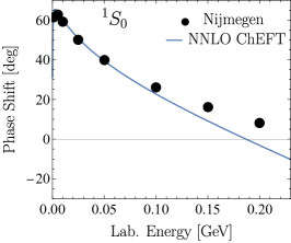
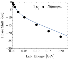
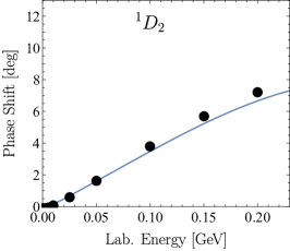
Figure 2: Spin-singlet NN phase shifts as functions of the laboratory energy. The results of Nijmegen PWA are shown by filled circles Stoks:1993tb . Solid lines correspond to the NNLO chiral EFT results Epelbaum:2003xx ; Epelbaum:2003gr .

To calculate phase shifts in the infinite volume, we solve the LSE in the CMF

$$T(\bm{p}^{\prime},\bm{p};E)=V(\bm{p}^{\prime},\bm{p};E)+\int\frac{d^{3}\bm{q}}{(2\pi)^{3}}\frac{V(\bm{p}^{\prime},\bm{q};E)\;T(\bm{q},\bm{p};E)}{E-\frac{\bm{q}^{2}}{m_{N}}+i\epsilon},$$ (33)

where $E$ is the energy of two nucleons and $m_{N}$ is the nucleon mass. Clearly, for infinite-volume calculations, it is more convenient to use the standard partial wave basis instead of solving the equation in real space. In figure 2, we compare the resulting neutron-proton phase shifts at NNLO with the ones from the Nijmegen partial wave analysis (PWA) Stoks:1993tb . This comparison clearly demonstrates that the NNLO potential already captures the most important features of the nuclear force.

Below, we will regard the chiral EFT potential introduced above as the underlying NN interaction to generate the corresponding FV energy spectra. We then compare our approach to reconstruct phase shifts from the FV energies with the single-channel Lüscher formula and explore FV effects due to partial wave mixing.

5.1 Lippmann-Schwinger equation in a finite volume

To solve the LSE in a finite volume, we employ the plane wave basis with quantized momenta instead of expanding it in partial waves. In the non-relativistic limit, eq. (8) reduces to

$$P_{d}^{\text{NR}}=\bigg{\{}\bm{n}-\frac{1}{2}\bm{d}\bigg{\}},\quad\bm{n}\in{Z}^{3}.$$ (34)

We define the matrices $\mathbb{T}$ and $\mathbb{G}$ according to

$$\mathbb{T}_{\bm{n}^{\prime},\bm{n}}=T\left(\frac{2\pi}{L}\bm{n}^{\prime},\frac{2\pi}{L}\bm{n};E\right),\quad\mathbb{G}_{\bm{n},\bm{n}^{\prime}}={\cal J}\frac{1}{L^{3}}\frac{1}{E-\frac{q_{\bm{n}}^{2}}{m_{N}}}\delta_{\bm{n}^{\prime},\bm{n}},\quad\bm{n},\bm{n}^{\prime}\in P_{d}^{\text{NR}}\,,$$ (35)

where $q_{\bm{n}}=2\pi\bm{n}/L$. Similarly, we define $\mathbb{V}_{\bm{n}^{\prime},\bm{n}}$. The integration has been replaced with the summation according to eq. (12). We introduce a truncation of the discretized momentum $q_{\bm{n}}<q_{\text{max}}$. For a non-relativistic theory, the Jacobi determinant is $\mathcal{J}=1$ and the LSE turns to a matrix equation

$$\mathbb{T=\mathbb{V}+\mathbb{V}\mathbb{G}\mathbb{T}}.$$ (36)

The poles of the $T$-matrix are obtained by solving equation

$$\det\left(\mathbb{G}^{-1}-\mathbb{V}\right)=0.~{}$$ (37)

If the potential is energy-dependent, the root-finding algorithm should be adopted. For energy-independent potentials, eq. (37) becomes an eigenvalue problem,

$$\det\left(\mathbb{H-}E\mathbb{I}\right)=0,\quad\text{with}\quad\mathbb{H}_{\bm{m},\bm{n}}=\frac{1}{L^{3}}\mathbb{V}_{\bm{m},\bm{n}}+\frac{q_{\bm{n}}^{2}}{m_{N}}\delta_{\bm{m},\bm{n}},$$ (38)

where $\mathbb{I}$ is the identity matrix. We see that the equation becomes a Hamiltonian equation. We, however, want to stress that this Hamiltonian equation is different from the one emerging in the approach of refs. Hall:2013qba ; Wu:2014vma ; Liu:2015ktc ; Li:2021mob . In that case, partial wave expansion was made prior to discretizing the magnitudes of the momenta. In our calculation, we discretize the momenta as three-vectors with no reliance on the partial wave expansion. For a related approach see ref. Mai:2019fba .

Using the projection operator technique described in section 3, we reduce the matrices in eq. (36) to block diagonal ones. Therefore, equation (38) turns into a set of matrix equations according to different irreps. The FV energy levels for a given irrep $\Gamma$ are then obtained by solving the eigenvalue problem for this irrep

$$\det\left(\mathbb{H}_{\Gamma}-E_{\Gamma}\mathbb{I}\right)=0,$$ (39)

where $\mathbb{H}_{\Gamma}$ belongs to the block of $\mathbb{H}$ corresponding to the irrep $\Gamma$.

5.2 The single-channel Lüscher method

We consider boxes of three different lengths: $L=3,5,8$ fm. In our calculations, we truncate the momentum at

$$q_{\text{max}}^{2}=100\left(2\pi\over L\right)^{2},$$ (40)

leading to $q_{\text{max}}\approx 4.1,2.5,1.5$ GeV for $L=3,5,8$ fm, respectively. These momenta are much larger than the cutoff parameter in the employed NN potential so that the solution of the LSE is well converged. We have verified that the error due to the truncation is negligibly small.

5.2.1 Benchmark calculation using contact interactions

To confirm the robustness of our approach, we first calculate the FV energy levels in pionless EFT. Specifically, we include the LO and NLO contact interactions, which contribute to the ¹S₀ and ¹P₁ channels. The coefficients in front of the contact interactions have been chosen the same as those in chiral EFT to the NNLO in ref. Epelbaum:2003xx . The regulators and cutoff parameters are introduced in eq. (32). The corresponding phase shifts, calculated by solving the LSE in the infinite volume and shown by solid lines in figure 3, feature a qualitatively similar behavior to the empirical ones in NN scattering.

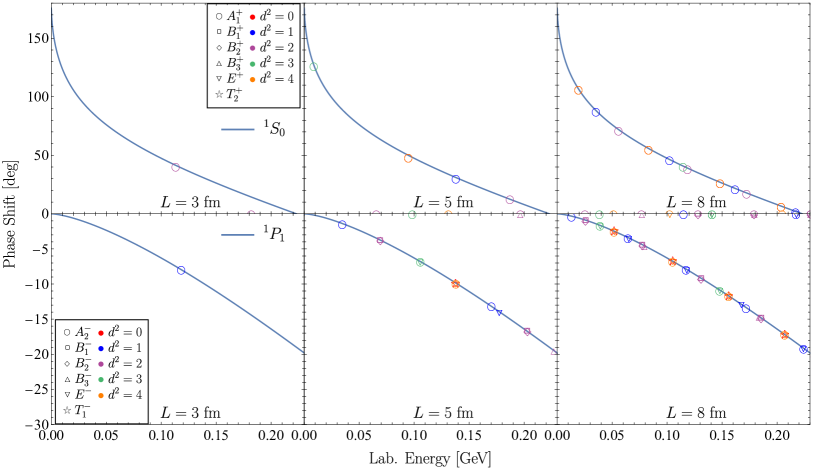
Figure 3: Upper (lower) row: Various symbols show the ¹S₀ (¹P₁) phase shifts calculated from the FV energy spectra using the single-channel Lüscher formula for the case of pionless EFT at NLO. Only those energy levels were used which belong to the irreps with the ¹S₀ or ¹P₁ components. Solid lines are the corresponding phase shifts calculated in the infinite volume. Left, middle and right graphs show the results obtained in the FV boxes with $L=3$, $5$ and $8$ fm, in order.

We then compute the FV energy levels by solving the LSE in the discretized plane wave basis as described in sections 3, 4. We regard the calculated energy spectra as synthetic data and apply the single-channel Lüscher formula to extract the phase shifts at these energies. The Lüscher quantization conditions are outlined in appendix B. The full quantization conditions are determinant equations involving all partial waves. In this study, we will refer to the approximation involving only a leading partial wave, which sets one-to-one relations between FV energy levels and phase shifts, as the single-channel Lüscher approach. In figure 3, the extracted ¹S₀ and ¹P₁ phase shifts in the boxes with $L=3,5,8$ fm are compared with the infinite-volume results. For the positive parity states, we only list the $A_{1}^{+}$ states, since the other irreps have no ¹S₀ components. With increased box sizes, the unit momentum $(2\pi/L)$ becomes smaller leading to denser energy spectra. In the infinite-volume limit, these discrete energy levels turn to the continuum spectrum. Meanwhile, one can see many energy levels corresponding to vanishing phase shifts (i.e. to the non-interacting case). In the FV, partial wave states with the same parity mix with each other due the violation of rotational symmetry. For example, the ¹S₀ states mix with the ¹D₂, ¹G₄, etc., ones. Thus, in general, energy levels with positive parity receive contributions from the interaction in the ¹S₀, ¹D₂ and even higher partial waves. Contact interactions at NLO, regularized with an angle-independent regulator, do, however, not contribute to D- and higher partial waves. Thus, the states in figure 3 with vanishing phase shifts correspond to the non-interacting ¹D₂, ¹F₃ and higher partial wave states. Apart from these points, the phase shifts calculated using the single-channel Lüscher formula are very close to the ones obtained in the infinite volume calculation. As expected, the single-channel Lüscher approach is found to work accurately for this case without partial wave mixing. Notice that since for the case at hand the range of the interaction is given by the inverse cutoff, the exponentially suppressed corrections to the Lüscher formula are negligible even for the smallest considered box size.

5.2.2 Chiral EFT at NNLO

We now turn to the realistic case and repeat the analysis outlined in the previous section for the chiral EFT NN interaction at NNLO. The results of our FV calculations are compared with those in the infinite volume in figure 4. Notice that for positive parity states, we only show the results using the $A_{1}^{+}$ irrep. We use the single-channel Lüscher formula suitable for the ¹S₀ partial wave in the case of the positive parity states and for the ¹P₁ partial wave in the case of the negative parity states. Obviously, for the realistic NN interaction at the physical pion mass, the single-channel Lüscher formula leads to significant deviations from the infinite volume calculations.

For positive-parity states shown in the upper row of figure 4, the deviation of single-channel Lüscher’s results from the exact ones is significant for the smallest considered box with $L=3$ fm. When the box size is increased to $5$ fm, the Lüscher single-channel formula performs reasonably well. Apart from the S-wave dominated states, one can identify several D-wave dominated states in figure 4 leading to smaller-in-magnitude phase shifts. Though we employ the Lüscher formula for the S-wave, its leading part $w_{00}$ is the same as that for the D-wave, see appendix B. Therefore, we obtain in figure 4 an approximation of the D-wave phase shift from D-wave-dominated states using the S-wave Lüscher formula.

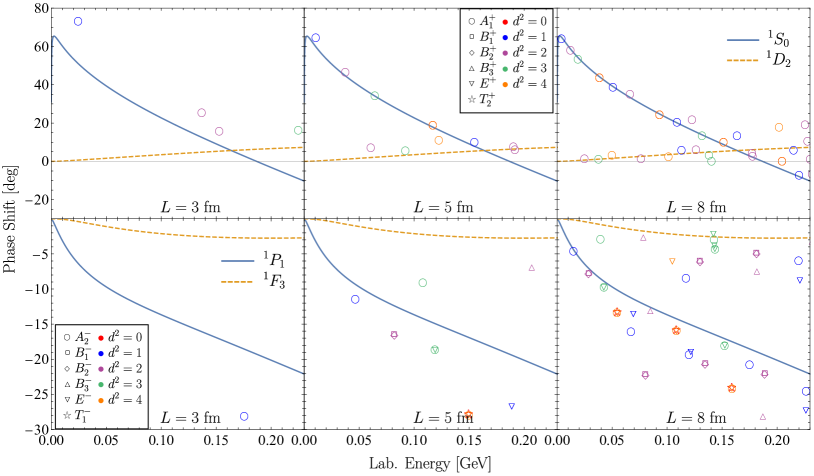
Figure 4: Upper (lower) row: Various symbols show positive-parity (negative-parity) phase shifts calculated from the FV energy spectra using the S-wave (P-wave) Lüscher formula for the chiral EFT potential at NNLO. Solid and dashed lines in the upper row (lower row) show the ¹S₀ and ¹D₂ (¹P₁ and ¹F₃) phase shifts, respectively, calculated in the infinite volume. For remaining notations see figure 3.

The states with negative parity in the lower row of  figure 4 are more interesting. Even for the largest considered box with $L=8$ fm, one observes large deviations from the infinite-volume results when using the single-channel Lüscher formula. One identifies two regions where the points are concentrated, namely well above the solid line (region-I) and below the solid line (region-II). One may expect the points in the region-I to emerge from states dominated by the F-wave (and possibly by even higher partial wave) interactions. The points in the region-II are found to gradually deviate from the exact result with increasing energies. Only in the very near-threshold region, the phase shifts for several energy levels are close to those from the infinite volume calculation. Notice that further increasing the box size is found to yield no improvement for the negative-parity phase shifts.

5.2.3 The one-pion-exchange potential

The results of the previous two sections suggest that the failure of the single-channel Lüscher formula for the NNLO chiral EFT potential is caused by partial wave mixing effects. For interactions with a finite non-zero range $R$, the near-threshold behavior of the phase shifts $\delta_{l}(p_{\rm on})$ with $E=p_{\rm on}^{2}/m_{N}$ is given by $\delta_{l}(p_{\rm on})\sim p_{\rm on}^{2l}$. This asymptotic expression, however, only applies to on-shell momenta well below the lowest $t$-channel singularity, i.e. for $p_{\rm on}<R^{-1}$. For the NN interaction, this restriction translates into $E_{\rm lab}\sim 2M_{\pi}^{2}/m_{N}\sim 10$ MeV. At such low energies, the single-channel Lüscher formula is expected to be valid since the contributions from higher partial waves are kinematically suppressed. This expectation is in line with the findings of the previous section for the largest considered box size. For $p_{\rm on}\gtrsim R^{-1}$, higher partial waves are still suppressed due to the centrifugal barrier, but the convergence of the partial wave expansion becomes slow. For example, to compute the NN differential cross section at $E_{\rm lab}=300$ MeV at the $1\%$ accuracy level, it is necessary to take into account partial waves up to the total orbital momentum of $j_{\rm max}=16$ Fachruddin:2001az . For very long-range interactions such as e.g. the magnetic moment interaction, the scattering amplitude is not converged even for $j_{\rm max}\sim 1000$ Stoks:1990us . One, therefore, may expect partial wave mixing effects in the FV calculations to be dominated by the longest-range OPE interaction. To get further insights into this issue and to validate this conjecture, we switch off all shorter-range interactions in the chiral EFT potential and consider the case of pure OPE.

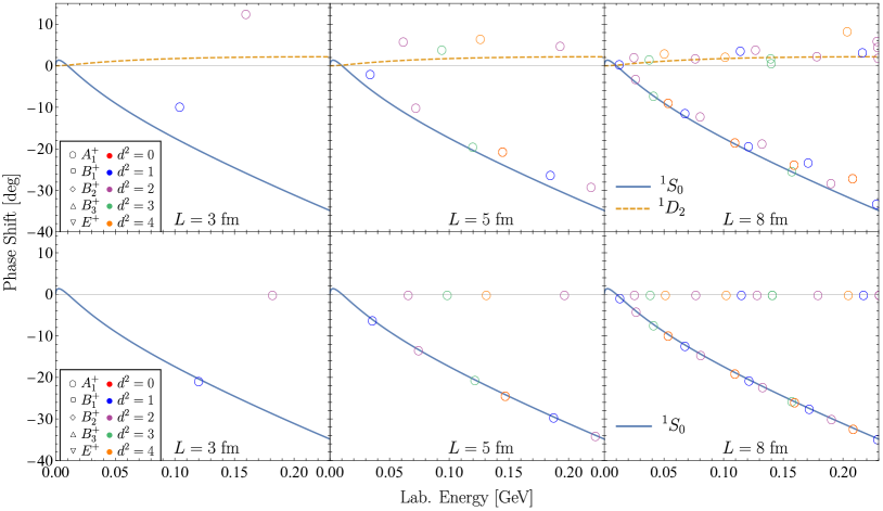
Figure 5: Phase shifts in the positive-parity channels extracted from the FV energy spectra using the S-wave Lüscher formula (various symbols) in comparison with the infinite-volume results for the OPE potential (upper row) and the S-wave projected OPE potential (lower row). Solid and dashed lines show the ¹S₀ and ¹D₂ phase shifts calculated in the infinite volume, respectively. For remaining notations see figure 3.

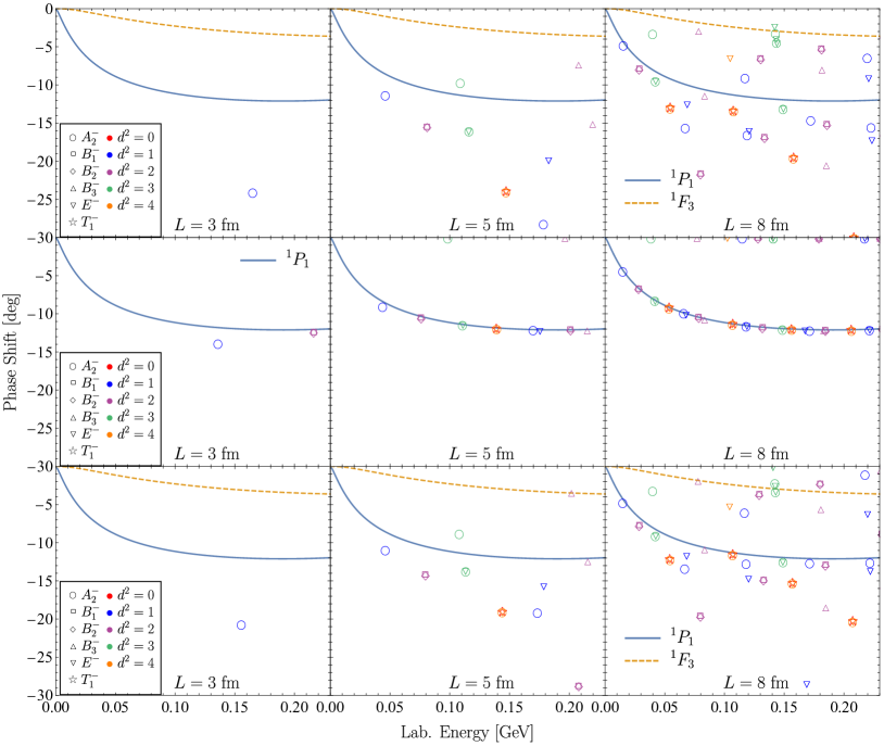
Figure 6: Phase shifts in the negative-parity channels extracted from the FV energy spectra using the P-wave Lüscher formula (various symbols) in comparison with the infinite-volume results for the OPE potential (upper row), the P-wave projected OPE potential (middle row) and the P- and F-wave projected OPE potential. Solid and dashed lines show the ¹P₁ and ¹F₃ phase shifts calculated in the infinite volume. For remaining notations see figure 3.

In the upper row of figures 5 and 6, we show the corresponding positive- and negative-parity phase shifts extracted from the FV energies using the single-channel Lüscher formula, along with the results in the infinite volume. The deviations in the obtained phase shifts are qualitatively similar to those found in the calculations based on the full NNLO chiral potential. For S-wave dominated states, the single-channel Lüscher formula gives rise to a significant deviation for the $L=3$ fm box, but it works reasonably well for $L\geq 5$ fm. This is in line with the findings of ref. Sato:2007ms . For P-wave dominated states, we again observe large deviations which persist even for the box size of $L=8$ fm. Meanwhile, the deviations are found to increase with energies.

We stress again that increasing the box size does not allow one to improve the results of the single-channel Lüscher formula at higher energies. For example, focusing on the energy levels around $0.15$ GeV in the first row of figure 6, one sees no obvious improvement of the results using the single-channel Lüscher method with increasing $L$. If one, however, considers the trajectory of a single state such as e.g.  the ground state of the $A_{2}^{-}$ irrep in the $\bm{d}^{2}=1$ system as a function of the box size, one does observe a significant improvement when it approaches the threshold region for a sufficiently large $L$.

To unambiguously identify partial wave mixing effects as the source of failure of the single-channel Lüscher formula, we consider the S-wave and P-wave projected OPE interaction. Specifically, we start with the partial wave expansion of the potential

$$V(\bm{p},\bm{p}^{\prime})=\sum_{l}\frac{2l+1}{4\pi}V_{l}(p,p^{\prime})P_{l}(z),$$ (41)

where $z=\cos\theta$ with $\theta$ being the angle between the initial and final momenta and $P_{l}(z)$ denotes the Legendre polynomial, and define the potentials $V_{\rm S-wave}(\bm{p},\bm{p}^{\prime})=(4\pi)^{-1}V_{0}(p,p^{\prime})P_{0}(z)$ and $V_{\rm P-wave}(\bm{p},\bm{p}^{\prime})=3(4\pi)^{-1}V_{1}(p,p^{\prime})P_{1}(z)$. Clearly, the resulting potentials do not generate any partial wave mixing effects when used to compute the FV energy spectra, so that the single-channel Lüscher approach is expected to become applicable. This is indeed fully consistent with our results, see the second rows in figures 5 and 6. For S-wave dominated states, the small deviation disappears after switching off the interaction in higher partial waves. For states with negative parity, the change is more pronounced. After switching off the interaction in higher partial waves, the P-wave phase shift is reproduced accurately with the single-channel Lüscher formula except for the smallest box size (presumably due to exponentially suppressed corrections).

Finally, the lower row in figure 6 shows the effect of including the F-wave interaction, i.e. we consider $V_{\rm P,F-wave}(\bm{p},\bm{p}^{\prime})=3(4\pi)^{-1}V_{1}(p,p^{\prime})P_{1}(z)+7(4\pi)^{-1}V_{3}(p,p^{\prime})P_{3}(z)$. While we have not explicitly investigated the impact of even higher partial waves, a comparison of the upper and lower rows in figure 6 suggests that their mixing effects may also be significant at higher energies.

5.3 Phase shifts from FV energies using EFT

In section 5.2, we have shown in detail that partial wave mixing effects can not be neglected when calculating FV energies of two interacting nucleons at the physical pion masses. Such large partial wave mixing effects are caused by the long-range (pion-exchange) interaction, and they are responsible for the failure of the single-channel Lüscher approach to extract phase shifts from FV energy spectra. This will pose a significant challenge for future lattice QCD calculations in the NN sector close to the physical point. In the lattice QCD community, the issue is addressed by including several partial waves in the Lüscher’s quantization conditions, see e.g. refs. Dudek:2012gj ; Cheung:2020mql . When more than one partial wave is included, there is no longer a one-to-one mapping between energy levels and phase shifts, and one has to choose a theoretical framework to parameterize the $T$-matrix. As an alternative to the Lüscher method, one can benefit from the known model-independent OPE interaction using an EFT-inspired approach. Specifically, we propose to determine the short-range part of the NN interaction, parametrized in a systematic way by means of contact interactions, via a direct matching to lattice QCD FV energy levels. The method is, to some extent, similar to the low-energy theorems used in refs. Baru:2015ira ; Baru:2016evv to restore the energy dependence of the NN scattering amplitude at unphysical pion masses.

To illustrate the method, we first define a toy model comprising the OPE and the heavy-meson-exchange potentials to generate synthetic data for the FV energies. Specifically, we consider

$$V_{\text{toy}}=V_{1\pi}+V_{1h}=-\left(\frac{g_{A}}{2F_{\pi}}\right)^{2}\frac{M_{\pi}^{2}}{\bm{q}^{2}+M_{\pi}^{2}}\bm{\tau}_{1}\cdot\bm{\tau}_{2}+\left(c_{h1}+c_{h2}\bm{\tau}_{1}\cdot\bm{\tau}_{2}\right){1\over\bm{q^{2}}+m_{h}^{2}},$$ (42)

where $V_{1\pi}$ is the OPE potential considered in the previous sections (up to an S-wave contact interaction). For the various parameters, we choose the numerical values of $M_{\pi}=139$ MeV, $F_{\pi}=92.4$ MeV and $g_{A}=1.26$. For the heavy-meson-exchange interaction, we introduce both the isospin-triplet and isospin-singlet potentials with the same meson mass $m_{h}=0.5$ GeV. Further, $c_{h1}$ and $c_{h2}$ denote the corresponding dimensionless coupling constants. In order to regularize the UV divergences, we introduce a nonlocal Gaussian cutoff

$$V_{\text{toy}}\;\to\;V_{\text{toy}}\;e^{-\frac{p^{2}+p^{\prime 2}}{\Lambda^{2}}},$$ (43)

and choose $\Lambda=0.45$ GeV. The couplings $c_{h1}$ and $c_{h2}$ are adjusted in such a way that the toy-model interaction mimics the behavior of the NN ¹S₀ and ¹P₁ phase shifts as shown in figure 7.

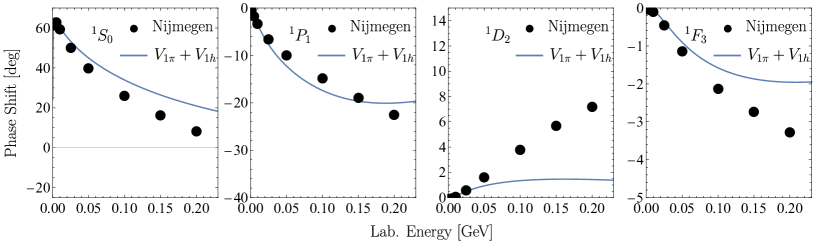
Figure 7: $S$, $P$, $D$ and F-wave phase shifts for the toy-model potential in eq. (41) in comparison with the corresponding spin-singlet NN phase shifts from the Nijmegen PWA Stoks:1993tb .

Using the toy model introduced above, we compute the corresponding FV energy levels, which are regarded as synthetic lattice data, see the right-most symbols in figures 8 and 9 for a given $\bm{d}^{2}$-value, where the results are only shown for the box with $L=5$ fm.

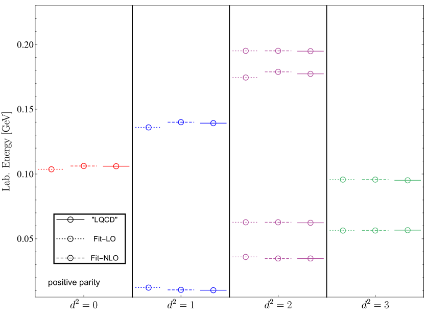
Figure 8: Comparisons of the synthetic lattice energy levels with positive parity in the box with $L=5$ fm and those from the EFT determined by fitting. The marker shapes represent the irreps, which are the same as those in figure 3.

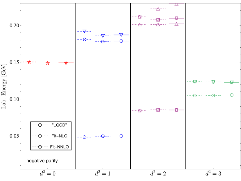
Figure 9: Comparison of the synthetic lattice energy levels with negative parity in the box with $L=5$ fm and those from the EFT determined by fitting. The marker shapes represent the irreps, which are the same as those in figure 3.

Having generated the synthetic data as described before, we are now in the position to describe our approach for extracting the corresponding phase shifts. To this aim, we exploit the knowledge of the long-range interaction in the underlying model to construct the EFT interaction

$$V_{\text{EFT}}=V_{\text{OPE}}^{(0)}+V_{\text{cont}}^{(0)}+V_{\text{cont}}^{(2)}+V_{\text{cont}}^{(4)}+...$$ (44)

We use the same regulator as in eq. (43) and employ the same value for the cutoff parameter $\Lambda=0.45$ GeV. In order to fit the FV energy levels with positive parity, we introduce the interaction at NLO,

$$V_{\text{cont}}^{(0)}=\frac{1}{4\pi}\tilde{C}_{{}^{1}S_{0}},\quad V_{\text{cont}}^{(2)}=\frac{1}{4\pi}C_{{}^{1}S_{0}}(p^{2}+p^{\prime 2})~{}.$$ (45)

where $\tilde{C}_{{}^{1}S_{0}}$ and $C_{{}^{1}S_{0}}$ refer to the corresponding LECs. For the states with negative parity, we include the contact interactions up to NNLO,

$$V_{\text{cont}}^{(2)}(p,p^{\prime},z)=\frac{3}{4\pi}C_{{}^{1}P_{1}}pp^{\prime}z,\quad V_{\text{cont}}^{(4)}(p,p^{\prime},z)=\frac{3}{4\pi}D_{{}^{1}P_{1}}pp^{\prime}(p^{2}+p^{\prime 2})z~{},$$ (46)

where $C_{{}^{1}P_{1}}$ and $D_{{}^{1}P_{1}}$ are the LECs. Since the contact interactions introduced above only contribute to the S- and P-wave channels, the FV partial wave mixing effects at the considered EFT order only arise from the OPE interaction.

To fix the LECs $\tilde{C}_{{}^{1}S_{0}}$, $C_{{}^{1}S_{0}}$, $C_{{}^{1}P_{1}}$ and $D_{{}^{1}P_{1}}$, we employ the determinant residual method. For the considered toy-model example, we neglect the uncertainties of the synthetic data. First, we perform single-parameter fits by including only the dominant contact interaction in the corresponding parity channel, i.e. at LO (NLO) for positive- (negative-) parity states. In the second step, we also take into account the corresponding subdominant contact terms and perform two-parameter fits to the FV energies. As for the synthetic data, we only include the ground state energy of each irrep as input. Meanwhile, we ignore the energy levels of the $\bm{d}=(0,0,2)$ systems because they are identical to those of the $\bm{d}=(0,0,0)$ system in the non-relativistic case. For positive-parity channels, this leaves us with three and four energy levels for the boxes with $L=3$ and $5$ fm, respectively, up to the maximal energy of 0.23 GeV. For the negative-parity case, we have one and eight energy levels for the boxes with $L=3$ and $5$ fm, respectively. Thus, for the smallest considered box size, our calculations for the negative-parity states are restricted to NLO in the EFT expansion due to the lack of input information.

In figures 8 and 9, we show the quality of the reproduction of the FV energy levels. The results from a single-parameter fit using the dominant contact interactions are shown by the dotted lines and the leftmost symbols for the considered $\bm{d}^{2}$ value, while the dashed lines with symbols in the middle correspond to two-parameter fits including the contributions of the subdominant contact terms. As expected, one observes a clear improvement in the description of the energy levels by including the subdominant short-range interactions. The largest deviations from the synthetic data are observed for higher-energy states, namely for the third $A_{1}^{+}$ state and the second $B_{3}^{-}$ state in the $\bm{d}^{2}=2$ box (which have not been used in the fits). This pattern is expected and reflects a slower convergence of the EFT at higher energies.

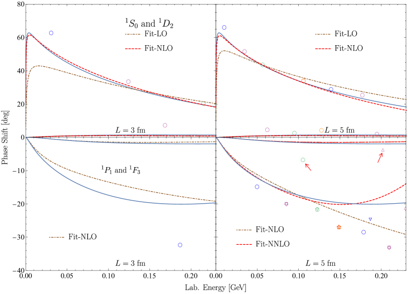
Figure 10: ¹S₀ (upper row) and ¹P₁ (lower row) phase shifts extracted by matching the EFT to the finite-volume spectra for the toy-model example in comparison with the underlying phase shifts shown by the solid blue lines. Brown dashed-dotted (red dashed) lines show the results from single-parameter (two-parameter) fits to the FV energies as visualized in figures  8 and 9. Left and right panels correspond to the boxes of the size $L=3$ fm and $L=5$ fm, respectively. Also shown by various symbols are the phase shifts extracted from the FV energies using the single-channel Lüscher formula. The lines near $\delta_{l}\sim 0$ show the phase shifts in the next-higher partial wave for a given parity quantum number (i.e. in the ¹D₂ and ¹F₃ channels in the upper and lower row, respectively). For remaining notations see figure 3.

Having determined the values of the LECs $\tilde{C}_{{}^{1}S_{0}}$, $C_{{}^{1}S_{0}}$, $C_{{}^{1}P_{1}}$ and $D_{{}^{1}P_{1}}$ from the FV spectra as discussed below, we are now in the position to compute the phase shifts. This is achieved by solving the partial wave LSE in the infinite volume using the standard methods. In figure 10, we compare the phase shifts resulting from matching the EFT in the finite volume with the ones from the underlying model. We also show in this figure the phase shifts extracted using the single-channel Lüscher formula. For the ¹S₀ channel, the one-parameter fit at LO only qualitatively captures the behavior of the underlying phase shift. This can be attributed to the strongly fine-tuned nature of the interaction in this channel as reflected by the very large absolute value of the scattering length and to the well-known important role played by the range corrections. The fit results at NLO are strongly improved, and the underlying phase shifts are correctly reproduced even using the smallest considered box size of $L=3$ fm. For the ¹P₁ channel, we only have a single data point for the smallest box at our disposal. Therefore, we can only perform a single-parameter fit for the $L=3$ fm box. Using the single channel Lüscher formula, the resulting phase shift deviates strongly from the underlying one, thus pointing towards a significant contribution of higher partial waves to this energy level. Nevertheless, in the approach we propose, the one-parameter fit to this energy level already allows one to capture the qualitative behavior of the phase shift in this channel. In the larger box with $L=5$ fm, we have more synthetic data at our disposal. The lower interacting energies as compared with the smaller box size allow for a more accurate determination of the LEC $C_{{}^{1}P_{1}}$ in the NLO fit, which results in an improved description of the phase shifts at low energies as compared with the one using the smaller box of $L=3$ fm. Including the subdominant contact interactions $\propto C_{{}^{1}S_{0}},\,D_{{}^{1}D_{2}}$, the description of both the ¹S₀ and ¹P₁ phase shifts improves considerably in a wide energy range. It should be emphasized that our input includes several energy levels dominated by higher partial wave components such as the ground state in the $A_{2}^{-}$ irrep with $\bm{d}^{2}=3$ and the ground state in the $B_{3}^{-}$ irrep with $\bm{d}^{2}=2$. Contrary to the single-channel Lüscher approach, which in these cases leads to large deviations, our method is insensitive to such FV partial wave mixing artifacts.

6 Application II: P-wave pion-pion scattering

We now turn to our second application and consider $\pi\pi$ scattering as an example of a relativistic system. In this exploratory example, we employ a simple phenomenological model for $\pi\pi$ interaction instead of using EFT. For a formulation of chiral perturbation theory with resonances see e.g. refs. Bernard:1991zc ; Bruns:2004tj .

6.1 Reduced Bethe-Salpeter equation in the finite volume

The relativistic Bethe-Salpeter equation is a four-dimensional integral equation. One has to reduce it into three-dimensional one to perform the plane wave expansion. In the literature, there are various approaches to achieve it Woloshyn:1973mce ; Kim:2005gf ; Albaladejo:2012jr . In this work, we choose the Blankenbecler-Sugar equation as discussed e.g. in ref. Woloshyn:1973mce as our starting point. One can analytically perform the integration over the $0$-th components of the relativistic two-body propagator as follows,

$${\cal G}=i\int\frac{d^{4}q}{(2\pi)^{4}}\frac{1}{(P-q)^{2}-M_{\pi}^{2}+i\epsilon}\frac{1}{q^{2}-M_{\pi}^{2}+i\epsilon}=i\int\frac{d^{3}\bm{q}}{(2\pi)^{3}}G(q;E),$$ (47)

with

$$G(q,E)=\frac{1}{2\omega_{1}(q)\omega_{2}(q)}\frac{\omega_{1}(q)+\omega_{2}(q)}{E^{2}-[\omega_{1}(q)+\omega_{2}(q)]^{2}+i\epsilon},$$ (48)

where $\omega_{i}(q)\equiv\sqrt{m_{i}^{2}+q^{2}}$ and $m_{1}=m_{2}=M_{\pi}$. The reduced BSE for the $\pi\pi$ scattering reads

$$T(\bm{p},\bm{p}^{\prime};E)=V(\bm{p},\bm{p}^{\prime};E)+i\int_{q<q_{\text{max}}}\frac{d^{3}\bm{q}}{(2\pi)^{3}}V(\bm{p},\bm{q};E)G(q;E)T(\bm{q},\bm{p}^{\prime};E).~{}$$ (49)

Notice that one can choose different reduced BSEs, but the procedure of performing the plane wave expansion is the same.

We expand the reduced BSE in the plane wave basis with discrete momenta to obtain the matrix equation

$$\mathbb{T}(E)=\mathbb{V}(E)+\mathbb{V}(E)\mathbb{G}(E)\mathbb{T}(E),$$ (50)

where the discretized propagator $\mathbb{G}$ is defined as

$$\mathbb{G}_{\bm{n},\bm{n}^{\prime}}={\cal J}\frac{1}{L^{3}}G(q_{\bm{n}},E)\delta_{\bm{n}^{\prime},\bm{n}}.$$ (51)

Further, $\mathcal{J}$ is the Jacobi determinant arising from the transformation between the BF and CMF as shown in eq. (12), which is given explicitly in eq. (13) for two different schemes. The FV energy levels are obtained by solving the determinant equation

$$\det\left[\mathbb{G}^{-1}(E)-\mathbb{V}(E)\right]=0.$$ (52)

The procedure for dealing with relativistic systems is more demanding than that for non-relativistic ones since the effective interaction $V$ in the three-dimensionally reduced eq. (49) is, in general, energy-dependent. Meanwhile, the Jacobi determinant can introduce additional energy-dependence. Such energy-dependence prevents one from reducing eq. (52) to the eigenvalue problem like in the non-relativistic case. In a special case when the interaction can be assumed to be energy-independent and the scheme-II is employed to relate the momenta in the BF and CMF as discussed in section 2.2, leading to the Jacobi determinant given in the second line of eq. (13), equation (52) reduces to the eigenvalue problem. This case is considered e.g. in refs. Hall:2013qba ; Wu:2014vma ; Liu:2015ktc ; Li:2021mob .

In this paper we do not make use of the above-mentioned simplifications and keep the energy dependence of the interaction and the Jacobi determinant. We decompose eq. (52) into decoupled matrix equations corresponding to different irreps. The FV energy levels are obtained by finding roots of the determinant equations for a given irrep $\Gamma$:

$$\det\left[\mathbb{G}^{-1}_{\Gamma}(E)-\mathbb{V}_{\Gamma}(E)\right]=0.$$ (53)

6.2 FV energy levels using a phenomenological model for P-wave $\pi\pi$ interaction

We employ a phenomenological interaction model for P-wave $\pi\pi$ scattering rather than chiral perturbation theory. Specifically, we parametrize the interaction via an energy-dependent potential

$$V(\bm{p},\bm{p}^{\prime};E)=-\frac{2\bm{p}\cdot\bm{p}^{\prime}}{f^{2}}\left(1+\frac{2G_{V}^{2}}{f^{2}}\frac{E^{2}}{M_{0}^{2}-E^{2}}\right),$$ (54)

where $f$, $M_{0}$ and $G_{V}$ are free parameters. We introduce the CDD (Castillejo, Dalitz, Dyson) pole in the interaction Castillejo:1955ed , which naturally appears in the description of the vector form factor of the $\pi\pi$ system Oller:2000ug based on the Lagrangians from refs. Gasser:1984gg ; Ecker:1988te . In this formalism, we neglect possible coupled-channel effects from the $K\bar{K}$ system. The interaction in eq. (54) corresponds to a short-range contact potential. The angular-dependent term $\bm{p}\cdot\bm{p}^{\prime}$ ensures that the interaction can only contribute to the P-wave, which switches off possible partial wave mixing effects in the finite volume. Thus, for such a short-range potential contributing to the P-wave alone, the single-channel Lüscher formula is perfectly applicable. The potential in the partial wave basis reads

$$V^{l=1}(p,p^{\prime};E)=-4\pi\frac{2pp^{\prime}}{3f^{2}}\left(1+\frac{2G_{V}^{2}}{f^{2}}\frac{E^{2}}{M_{0}^{2}-E^{2}}\right).$$ (55)

Notice that if we would make an on-shell approximation, we would obtain the interaction of ref. Chen:2012rp (up to the $4\pi$-factor), which was used to investigate finite volume effects in the same channel within the chiral unitary approach. In our normalization, the phase shift can be extracted from the partial wave $T$-matrix as

$$T^{l}(E)=\frac{-32\pi^{2}E}{p\cot\delta^{l}-ip}.$$ (56)

Recently, lattice simulations of $\pi\pi$ scattering in the $\rho$-channel at the physical value of the pion mass were performed Fischer:2020fvl . In our calculation, we choose the same box size of $L=4.3872$ fm and pion mass of $M_{\pi}=132$ MeV as used in that work. Since the root-finding algorithm is very time-consuming, we choose a smaller cutoff $q_{\text{max}}=1.5$ GeV as compared to the one employed in ref. Chen:2012rp . The three parameters $f$, $M_{0}$ and $G_{V}$ are determined by fitting the experimental $\pi\pi$ scattering phase shift Estabrooks:1974vu ; Protopopescu:1973sh leading to the values of

$$f=0.124\text{ GeV},\quad\quad G_{V}=0.059\text{ GeV},\quad\quad M_{0}=1.110\text{ GeV}.$$ (57)

In figure 11, we show that the resulting phase shifts from our model provide a very good description of the experimental ones.

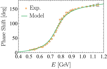
Figure 11: P-wave $\pi\pi$ phase shifts of the phenomenological model defined in eq. (54) (solid line) in comparison with the experimental data from refs. Estabrooks:1974vu ; Protopopescu:1973sh (open dots).

Using the constructed model, we compute the FV energy levels of the $\pi\pi$ system in two different schemes to discretize the momenta as discussed in subsection 2.2. We then extract the phase shifts corresponding to these FV energy levels using the single-channel Lüscher formula as shown in figure 12. As expected, for the considered short-range interaction without partial waving mixing, the single-channel Lüscher formula leads to accurate results, which holds true for both considered discretization schemes. The outlier points with phase shifts about 180 degrees correspond to the non-interacting higher partial wave components. Further, in figure 13 we compare our calculated FV energy levels with those from lattice QCD simulations Fischer:2020fvl ; data . The differences of the FV energy levels from two discretization schemes appear to be tiny. Meanwhile, one can see the clear correspondence between our calculation and lattice QCD results for the low-lying energy levels in each irrep. For states below the inelastic threshold $4M_{\pi}$, our results are close to the lattice QCD ones.

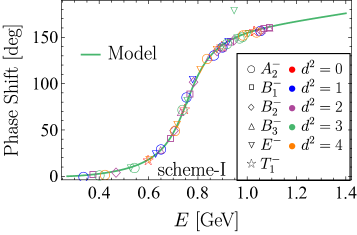
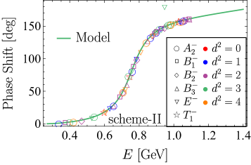
Figure 12: P-wave $\pi\pi$ phase shifts of the phenomenological model defined in eq. (54) (solid lines) in comparison with the phase shifts extracted from the FV energies using the single-channel Lüscher formula (various symbols). Left and right panels correspond to two different schemes for discretizing the momenta in the moving frames as explained in section 2.2.

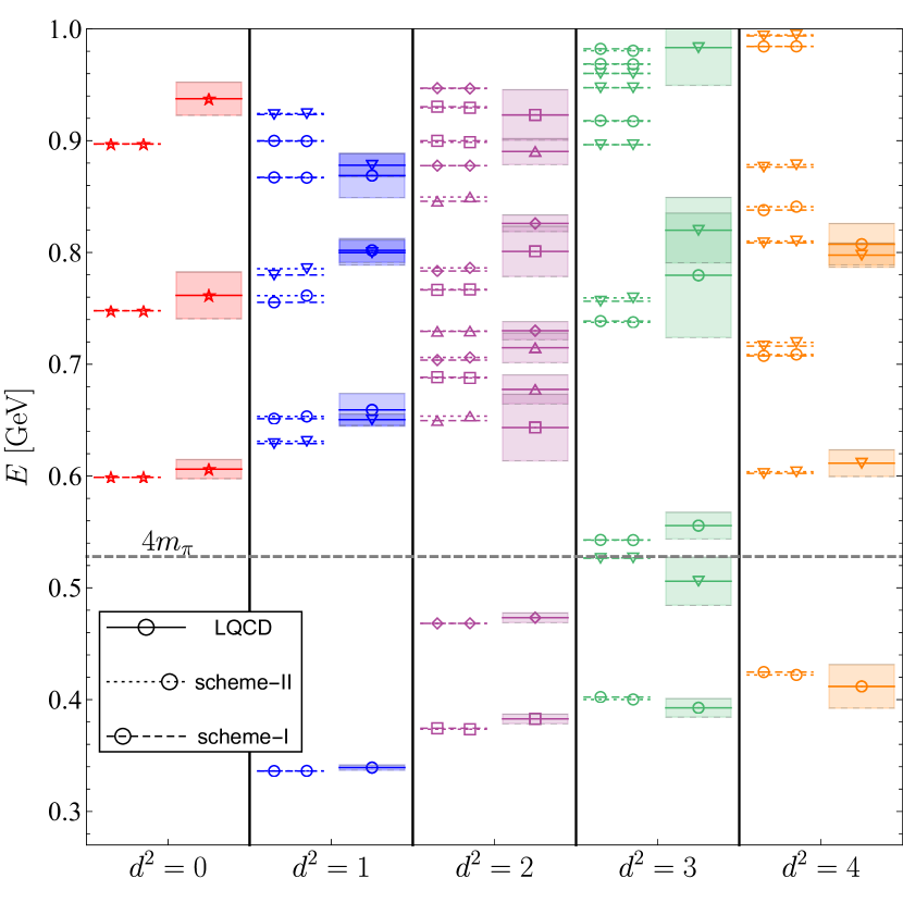
Figure 13: Comparison of the FV energy levels from lattice QCD and our calculations using the two different schemes for discretizing the momenta in the moving frames as explained in section 2.2. The notation for various symbols is the same as those in figure 12. The uncertainties of the lattice QCD data are taken from ref. data .

6.3 P-wave $\pi\pi$ scattering from lattice QCD data for FV energies

We are now in the position to apply our approach for extracting the phase shifts from the FV spectra by fixing the model parameters $f$, $G_{V}$ and $M_{0}$ directly from the lattice QCD energy levels. To this end, we adopt the determinant residual method Morningstar:2017spu and use the six energy levels below the $4M_{\pi}$ threshold from the lattice QCD simulations of ref. Fischer:2020fvl shown in figure 13.

We define the $\chi^{2}$-function as in eq. (26). To calculate the uncertainties $\sigma[\Omega_{\Gamma}(E_{\Gamma,i})]$, one should propagate the errors of the energy levels from lattice QCD to the residual function $\Omega_{\Gamma}(E_{\Gamma,i})$, which is a tedious and time-consuming task. In our exploratory calculation we neglect possible correlations among the lattice data, which will have to be taken into account for more precise determinations of the phase shifts in future studies, and make an approximation

$$\sigma[\Omega_{\Gamma}(E_{\Gamma,i})]\approx\frac{1}{2}\left|\Omega(E_{\Gamma,i}^{\text{upper}})-\Omega(E_{\Gamma,i}^{\text{lower}})\right|,$$ (58)

where $E_{\Gamma,i}^{\text{upper}}$ and $E_{\Gamma,i}^{\text{lower}}$ are the upper and lower limits of the energy levels from the lattice data. We use the discretization scheme-I to fit the lattice QCD energy levels. We minimize the $\chi^{2}$-function using the package MINUIT James:1994vla and obtain

$$f=118.6\pm 8.3\text{ MeV},\quad\quad M_{0}=1230.8\pm 94.0\text{ MeV},\quad\quad G_{V}=53.3\pm 5.4\text{ MeV}.$$ (59)

Having extracted the parameters of the model from the lattice QCD FV energy levels, we calculate the $\pi\pi$ P-wave phase shifts by solving the reduced BSE for the $T$-matrix in the infinite volume. In figure  14, the resulting phase shifts are shown, along with the uncertainty stemming from the errors in the extracted values of the model parameters in eq. (59). The pole mass and width extracted from our fitting results read,

$$M=754^{+189}_{-195}\text{ MeV},\quad\Gamma=247^{+114}_{-107}\text{ MeV}.$$ (60)

As a comparison, the mass and width obtained within the inverse amplitude method in ref. Fischer:2020fvl are 786(20) MeV and 180(6) MeV, respectively. Though the uncertainties of the extracted phase shifts, mass and widths appear to be large, owing to the employed simplistic model and the restriction of the used lattice QCD data to energies below the first inelastic channel, these results confirm that our method can also be successfully applied to relativistic systems.

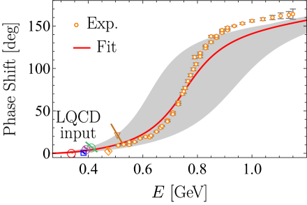
Figure 14: P-wave $\pi\pi$ phase shifts extracted by matching the phenomenological model to the FV energy levels below the first inelastic channel computed in lattice QCD Fischer:2020fvl . Experimental data are taken from refs. Estabrooks:1974vu ; Protopopescu:1973sh . The red line shows the central result of the fit with the shaded area representing the fit uncertainty. The six lattice QCD energy levels with uncertainties are shown by various open symbols using the same notation as in figure 12.

7 Summary and outlook

In this work, we propose an alternative approach to Lüscher’s method for extracting two-body scattering information from FV energy levels. We employ the plane wave basis instead of relying on the commonly used partial wave expansion. Using the projection operator technique, we reduce the discrete plane wave basis into a direct sum of irreducible representations of the corresponding discrete groups. The FV energy levels are computed by solving the LSE or BSE for nonrelativistic or relativistic systems, respectively, for a given irrep and finding the poles of the resulting amplitude. The formalism is applied to both static and moving two-particle systems in finite periodic boxes. Since we do not use the partial wave expansion, all partial wave mixing effects due to rotational symmetry breaking in a cubic box are naturally embedded.

We have used the above method to study spin-singlet NN scattering below pion production threshold as an example of a nonrelativistic system. Specifically, our goal was to study the impact of the long-range interaction due to the one-pion exchange on the severity of partial wave mixing effects when using the Lüscher formula to relate scattering phase shifts and FV energy levels. Throughout this study, we have restricted ourselves to the physical value of the pion mass. For S-wave dominated states, we found the single-channel Lüscher formula to lead to significant deviations for the smallest considered box size of $L=3$ fm. For larger boxes with $L\gtrsim 5$ fm, the ¹S₀ phase shift is, however, well reproduced for energies below $E_{\rm lab}\lesssim 150$ MeV, indicating that the contributions of the ¹D₂ and higher partial waves to the corresponding FV energy levels are negligible. On the other hand, we found severe partial wave mixing effects for P-wave dominated states, which originate from the longest-range interaction due to the OPE and make the single-channel Lüscher method inapplicable regardless of the considered box size (except for the near-threshold kinematics). While present-day lattice QCD calculations of the NN system are limited to unphysically large pion masses, this issue will pose a challenge once the lattice results will get closer to the physical point.

A natural and efficient solution to this problem can be achieved using the EFT framework, as it allows one to take into account the implications of long-range interactions in a systematic and model-independent way. To illustrate the method, we have considered a toy model of the NN interaction comprising the long-range OPE accompanied by the heavy-meson exchange potentials, which reproduces the qualitative behavior of the ¹S₀ and ¹P₁ neutron-proton phase shifts. In the absence of lattice QCD results for the NN system near the physical point, we used this model to generate synthetic data for FV energy levels. We then constructed the corresponding EFT featuring the same long-range interaction due to the OPE and involving contact terms with an increasing number of derivatives. Having determined the corresponding LECs by fitting them to the synthetic lattice QCD data, we have succeeded to reproduce the phase shifts of the underlying model using even the smallest box of $L=3$ fm. All FV calculations are carried out using the discretized plane wave basis. The accuracy of the resulting phase shifts is systematically improvable by going to higher orders in the EFT expansion, and the method is completely insensitive to partial wave mixing effects that plague the applications of the Lüscher formula. Our results suggest that a precise determination of spin-singlet NN phase shifts from lattice QCD simulations at the physical point should be possible with box sizes no larger than $L\sim 4\ldots 5$ fm. The lower bound on the box size in our approach is set by the requirement to have a sufficient number of resolved energy levels within the EFT applicability domain rather than by the interaction range as it is the case for the Lüscher approach.

As a second application, we considered P-wave $\pi\pi$ scattering. Partial wave mixing effects are not expected to be an issue for the $\pi\pi$ system in the FV, and our main motivation here was to demonstrate the applicability of our method in a relativistic setting. We employed a phenomenological model to parametrize the $\pi\pi$ interaction instead of relying on EFT. The three adjustable parameters of the model were tuned to reproduce the experimental behavior of the P-wave phase shift. We then computed the FV energy levels using the plane wave basis and compared them with those from lattice QCD simulations for the same pion mass and box size, finding a good agreement for the low-lying states in every irrep. We also applied our method to extract the phase shift by tuning the parameters of the model directly to the lattice QCD energy levels below the four-pion threshold. Though the uncertainties in the resulting determination are large, our central results agree well with the experimental $\pi\pi$ scattering phase shifts.

The considered examples provide a proof-of-principle that our approach can be successfully employed to extract the infinite-volume scattering information from FV energy levels accessible in lattice QCD. The essential ingredients of our method are (i) EFT or, possibly, phenomenological approaches to parametrize the interaction between the considered particles in a systematic way, (ii) the plane-wave basis in momentum space to avoid complications caused by partial wave mixing in the FV and (iii) matching to the FV energy spectra computable in lattice QCD. Compared with the conventional Lüscher approach, our method offers the advantage of being insensitive to partial wave mixing artifacts in the FV energy levels, and it also allows one to considerably reduce the box size by taking into account exponentially suppressed corrections to the Lüscher formula in the cases where the long-range interaction is known. Compared to alternative schemes discussed in literature such as the FV unitarized chiral perturbation theory for Goldstone boson scattering Doring:2011vk ; Doring:2012eu and the effective Hamiltonian approach of refs. Hall:2013qba ; Wu:2014vma ; Liu:2015ktc ; Li:2021mob , our method allows for a clean decomposition of two-particle states into irreps of the FV symmetry groups and does not rely on the partial wave expansion known to converge slowly in the presence of long-range interactions. We have also addressed the complication due to a possible energy dependence of the effective interactions. In that case, one has to resort to the root-finding algorithm to obtain the poles of the $T$-matrix, which is computationally time consuming. We have explored an alternative technique to speed up the calculations by using the determinant residual method when tuning the parameters of the interaction to the FV energies.

The method contains two different ingredients, the EFT as the dynamics framework and plane wave expansion as the tool for numerical solution of FV energy levels. One can choose to combine one of them with other frameworks. For example, the plane wave expansion method in this work can be used to obtain the FV energy levels in the interaction of refs. Wu:2014vma ; Liu:2015ktc . The EFT framework in this work can be used to parameterize the multi-channel Lüscher quantization conditions. At the cost of more numerical effect, one might expect similar results to those in this work if the partial wave expansion is truncated such that the expansion of the amplitudes converges below a given energy. In the partial wave expansion, one should use the infinite-volume EFT framework to calculate NN phase shifts in different partial waves and then write down the multi-channel Lüscher equation containing all these partial waves. Using plane wave expansion, one can write down the FV quantization conditions directly without considering the scattering in infinite volume, which saves considerable effort.

As already pointed out above, we expect our method to show largest benefits for lattice QCD studies of systems featuring long-range interactions such as e.g. nucleon-nucleon scattering with the pion mass near or even smaller than the physical value. In the past few years, chiral EFT for the two-nucleon system has been developed into a precision tool, see e.g. Reinert:2017usi ; Reinert:2020mcu ; Filin:2019eoe ; Filin:2020tcs for recent precision studies. In ref. Reinert:2020mcu , a full fledged partial wave analysis of the available neutron-proton and proton-proton scattering data up to the pion production threshold has, for the first time, been performed within the framework of chiral EFT, thereby achieving a statistically perfect description of the experimental data. However, away from the physical quark masses, no experimental data are available, and one will have to rely on lattice QCD simulations, see NPLQCD:2011naw ; Inoue:2011ai ; Yamazaki:2012hi ; Yamazaki:2015asa ; Orginos:2015aya ; Horz:2020zvv for examples of lattice QCD studies in the NN sector and ref. Davoudi:2020ngi for a recent review article. For heavy pion masses NPLQCD:2012mex ; Yamazaki:2012hi , lattice QCD results have already been matched to pionless EFT Barnea:2013uqa , see also ref. Drischler:2019xuo ; Davoudi:2020ngi . Our study provides a first step towards establishing an efficient and robust interface between lattice QCD and chiral EFT that will become necessary once the simulations at lower pion masses will become available. While we have restricted ourselves to spinless systems of two particles with equal masses in the present work, a generalization to nonzero spin and to particles with different masses in elongated boxes is straightforward. Work along these lines is in progress.

Appendix A Discrete groups

In this appendix, we briefly describe the elements, conjugacy classes and characters of the $O_{h}$, $D_{4h}$, $D_{2h}$ and $D_{3d}$ groups needed in our analysis. For more details see textbooks about point groups, such as e.g. ref. dresselhaus2007group . In table 5 the elements and conjugacy classes of the point group $O$ are presented. We label the $24$ rotation elements as $R_{1},...,R_{24}$. The elements of $O_{h}$ can be obtained by using $O_{h}=O\otimes\{E,I\}$. The character tables of $O_{h}$ and $O$ are presented in tables 6 and  7, respectively. The elements and characters of $D_{4}$, $D_{2}$ and $D_{3}$ groups are given in tables 8, 9 and 10, respectively. The group elements and characters of $D_{4h}$, $D_{2h}$ and $D_{3d}$ can be obtained easily.

Class	$R_{i}$	${\bm{n}}$	$\omega$	$\alpha$	$\beta$	$\gamma$	$|R_{i}\bm{p}\rangle$
$E$	$R_{1}$	any	$0$	$0$	$0$	$0$	$|p_{x},p_{y},p_{z}\rangle$
$8C_{3}$	$R_{2}$	$(1,1,1)$	$-2\pi/3$	$-\pi/2$	$-\pi/2$	$0$	$|p_{y},p_{z},p_{x}\rangle$
	$R_{3}$	$(1,1,1)$	$2\pi/3$	$0$	$\pi/2$	$\pi/2$	$|p_{z},p_{x},p_{y}\rangle$
	$R_{4}$	$(-1,1,1)$	$-2\pi/3$	$0$	$-\pi/2$	$-\pi/2$	$|-p_{z},-p_{x},p_{y}\rangle$
	$R_{5}$	$(-1,1,1)$	$2\pi/3$	$\pi/2$	$\pi/2$	$0$	$|-p_{y},p_{z},-p_{x}\rangle$
	$R_{6}$	$(-1,-1,1)$	$-2\pi/3$	$-\pi/2$	$\pi/2$	$0$	$|p_{y},-p_{z},-p_{x}\rangle$
	$R_{7}$	$(-1,-1,1)$	$2\pi/3$	$0$	$-\pi/2$	$\pi/2$	$|-p_{z},p_{x},-p_{y}\rangle$
	$R_{8}$	$(1,-1,1)$	$-2\pi/3$	$0$	$\pi/2$	$-\pi/2$	$|p_{z},-p_{x},-p_{y}\rangle$
	$R_{9}$	$(1,-1,1)$	$2\pi/3$	$\pi/2$	$-\pi/2$	$0$	$|-p_{y},-p_{z},p_{x}\rangle$
$6C_{4}$	$R_{10}$	$(1,0,0)$	$-\pi/2$	$-\pi/2$	$-\pi/2$	$\pi/2$	$|p_{x},p_{z},-p_{y}\rangle$
	$R_{11}$	$(1,0,0)$	$\pi/2$	$\pi/2$	$-\pi/2$	$-\pi/2$	$|p_{x},-p_{z},p_{y}\rangle$
	$R_{12}$	$(0,1,0)$	$-\pi/2$	$0$	$-\pi/2$	$0$	$|-p_{z},p_{y},p_{x}\rangle$
	$R_{13}$	$(0,1,0)$	$\pi/2$	$0$	$\pi/2$	$0$	$|p_{z},p_{y},-p_{x}\rangle$
	$R_{14}$	$(0,0,1)$	$-\pi/2$	$-\pi/2$	$0$	$0$	$|p_{y},-p_{x},p_{z}\rangle$
	$R_{15}$	$(0,0,1)$	$\pi/2$	$\pi/2$	$0$	$0$	$|-p_{y},p_{x},p_{z}\rangle$
$6C^{\prime}_{2}$	$R_{16}$	$(0,1,1)$	$-\pi$	$-\pi/2$	$-\pi/2$	$-\pi/2$	$|-p_{x},p_{z},p_{y}\rangle$
	$R_{17}$	$(0,-1,1)$	$-\pi$	$-\pi/2$	$\pi/2$	$-\pi/2$	$|-p_{x},-p_{z},-p_{y}\rangle$
	$R_{18}$	$(1,1,0)$	$-\pi$	$-\pi/2$	$-\pi$	$0$	$|p_{y},p_{x},-p_{z}\rangle$
	$R_{19}$	$(1,-1,0)$	$-\pi$	$0$	$\pi$	$-\pi/2$	$|-p_{y},-p_{x},-p_{z}\rangle$
	$R_{20}$	$(1,0,1)$	$-\pi$	$0$	$\pi/2$	$-\pi$	$|p_{z},-p_{y},p_{x}\rangle$
	$R_{21}$	$(-1,0,1)$	$-\pi$	$0$	$-\pi/2$	$-\pi$	$|-p_{z},-p_{y},-p_{x}\rangle$
$3C_{2}=3C_{4}^{2}$	$R_{22}$	$(1,0,0)$	$-\pi$	$\pi$	$\pi$	$0$	$|p_{x},-p_{y},-p_{z}\rangle$
	$R_{23}$	$(0,1,0)$	$-\pi$	$0$	$-\pi$	$0$	$|-p_{x},p_{y},-p_{z}\rangle$
	$R_{24}$	$(0,0,1)$	$-\pi$	$0$	$0$	$-\pi$	$|-p_{x},-p_{y},p_{z}\rangle$

Table 5: Elements and conjugacy classes of the O group. The rotations are parametrized by the rotation axis $\bm{n}$ and angle $\omega$ or by the Euler angles $\alpha,\beta,\gamma$.

	$E$	$8C_{3}$	$6C_{4}$	$6C^{\prime}_{2}$	$3C_{2}=3C_{4}^{2}$
$A_{1}$	1	1	1	1	1
$A_{2}$	1	1	-1	-1	1
$E$	2	-1	0	0	2
$T_{1}$	3	0	1	-1	-1
$T_{2}$	3	0	-1	1	-1

Table 6: Character table for the $O$ group.

	$E$	$\cdots$	$3C_{2}$	$I$	$\cdots$	$3IC_{2}$
$A_{1}^{+}$
$\vdots$		$\chi(O)$			$\mathbb{\chi}(O)$
$T_{2}^{+}$
$A_{1}^{-}$
$\vdots$		$\mathbb{\chi}(O)$			$-\mathbb{\chi}(O)$
$T_{2}^{-}$

Table 7: Character table for the $O_{h}$ group. $\chi(O)$ stands for the character table of the $O$ group given in table 6.

$D_{4}$ group	$R_{1}$	$R_{24}$	$R_{14},R_{15}$	$R_{22},R_{23}$	$R_{18},R_{19}$
	$E$	$C_{2}=C_{4}^{2}$	$2C_{4}$	$2C_{2}^{\prime}$	$2C_{2}^{\prime\prime}$
$A_{1}$	1	1	1	1	1
$A_{2}$	1	1	1	-1	-1
$B_{1}$	1	1	-1	1	-1
$B_{2}$	1	1	-1	-1	1
$E$	2	-2	0	0	0

Table 8: Character table for the $D_{4}$ group. The group elements $R_{i}$ are listed in table 5.

$D_{2}$ group	$R_{1}$	$R_{18}$	$R_{19}$	$R_{24}$
	$E$	$C_{2}(e_{x}+e_{y})$	$C_{2}(e_{x}-e_{y})$	$C_{2}(e_{z})$
$A_{1}$	1	1	1	1
$B_{1}$	1	1	-1	-1
$B_{2}$	1	-1	1	-1
$B_{3}$	1	-1	-1	1

Table 9: Character table for the $D_{2}$ group. The group elements $R_{i}$ are listed in table 5.

$D_{3}$ group	$R_{1}$	$R_{2},R_{3}$	$R_{17},R_{19},R_{21}$
	$E$	$2C_{3}$	$3C_{2}^{\prime}$
$A_{1}$	1	1	1
$A_{2}$	1	1	-1
$E$	2	-1	0

Table 10: Character table for the $D_{3}$ group. The group elements $R_{i}$ are listed in table 5.

Appendix B Lüscher quantization conditions

For the spinless systems, the Lüscher quantization conditions read Gockeler:2012yj ,

$$\det\left[M_{ln,l^{\prime}n^{\prime}}^{(\Gamma,\bm{P})}-\delta_{ll^{\prime}}\delta_{nn^{\prime}}\cot\delta_{l}\right]=0,$$ (61)

where, $l$ and $l^{\prime}$ are the angular momentum quantum numbers, $n$ and $n^{\prime}$ are used to label the multiple occurrences of $\Gamma$ in the representation spaces with the angular momentum $l$ and $l^{\prime}$, while $M_{ln,l^{\prime}n^{\prime}}^{(\Gamma,\bm{P})}$ is the interaction-independent matrix. For two-body systems of particles with equal masses, we list the matrix elements $M_{ln,l^{\prime}n^{\prime}}^{(\Gamma,\bm{P})}$ with positive and negative parities in tables 11 and 12, respectively. In principle, $M_{ln,l^{\prime}n^{\prime}}^{(\Gamma,\bm{P})}$ is an infinite-dimensional matrix. We truncate the angular momenta to $l\leq 2$. To make the expression concise, we adopt the short-hand notation,

$$w_{lm}=\frac{1}{\pi^{3/2}\sqrt{2l+1}}\gamma^{-1}q^{-l-1}{\cal Z}_{lm}^{\bm{P}}(1,q^{2}),$$ (62)

where ${\cal Z}_{lm}^{\bm{P}}(1,q^{2})$ are the conventional Lüscher zeta functions, which can be evaluated numerically Leskovec:2012gb .

$\bm{d}$	$\Gamma$-I	$\Gamma$-II	$M^{(\Gamma_{i},\bm{P})}$	Partial wave
$(0,0,0)$	$A_{1}^{+}$	$A_{1}^{+}$	$\left[w_{00}\right]$	$\{S\}$
	$E^{+}$	$E^{+}$	$\left[w_{00}+\frac{18}{7}w_{40}\right]$	$\{D\}$
	$T_{2}^{+}$	$T_{2}^{+}$	$\left[w_{00}-\frac{12}{7}w_{40}\right]$	$\{D\}$
$(0,0,a)$	$A_{1}^{+}$	$A_{1}^{+}$	$\left[\begin{array}[]{cc}w_{00}&-\sqrt{5}w_{20}\\ -\sqrt{5}w_{20}&w_{00}+\frac{10}{7}w_{20}+\frac{18}{7}w_{40}\end{array}\right]$	$\{S,D\}$
	$B_{1}^{+}$	$B_{1}^{+}$	$\left[w_{00}-\frac{10}{7}w_{20}+\frac{3}{7}w_{40}+\frac{3\sqrt{70}}{7}w_{44}\right]$	$\{D\}$
	$B_{2}^{+}$	$B_{2}^{+}$	$\left[w_{00}-\frac{10}{7}w_{20}+\frac{3}{7}w_{40}-\frac{3\sqrt{70}}{7}w_{44}\right]$	$\{D\}$
	$E^{+}$	$E^{+}$	$\left[w_{00}+\frac{5}{7}w_{20}-\frac{12}{7}w_{40}\right]$	$\{D\}$
$(a,a,0)$	$A_{1}^{+}$	$A_{1}^{+}$	$\left[\begin{array}[]{ccc}w_{00}&\sqrt{10}w_{22}&-\sqrt{5}w_{20}\\ -\sqrt{10}w_{22}&A_{22}&A_{23}\\ -\sqrt{5}w_{20}&-A_{23}&A_{33}\end{array}\right]$	$\{S,D_{a},D_{b}\}$
			$\begin{array}[]{cl}A_{22}&=w_{00}-\frac{10}{7}w_{20}+\frac{3}{7}w_{40}-\frac{3\sqrt{70}}{7}w_{44}\\ A_{33}&=w_{00}+\frac{10}{7}w_{20}+\frac{18}{7}w_{40}\\ A_{23}&=-\frac{10\sqrt{2}}{7}w_{22}+\frac{3\sqrt{30}}{7}w_{42}\end{array}$
	$B_{1}^{+}$	$A_{2}^{+}$	$\left[w_{00}+\frac{5}{7}w_{20}-\frac{12}{7}w_{40}+i\frac{5\sqrt{6}}{7}w_{22}+i\frac{6\sqrt{10}}{7}w_{42}\right]$	$\{D\}$
	$B_{2}^{+}$	$B_{1}^{+}$	$\left[w_{00}+\frac{5}{7}w_{20}-\frac{12}{7}w_{40}-i\frac{5\sqrt{6}}{7}w_{22}-i\frac{6\sqrt{10}}{7}w_{42}\right]$	$\{D\}$
	$B_{3}^{+}$	$B_{2}^{+}$	$\left[w_{00}-\frac{10}{7}w_{20}+\frac{3}{7}w_{40}+\frac{3\sqrt{70}}{4}w_{44}\right]$	$\{D\}$
($a,a,a)$	$A_{1}^{+}$	$A_{1}^{+}$	$\left[\begin{array}[]{cc}w_{00}&\sqrt{30}w_{22}\\ -\sqrt{30}w_{22}&A_{22}\end{array}\right]$	$\{S,D\}$
			$A_{22}=w_{00}-\frac{12}{7}w_{40}-i\frac{10\sqrt{6}}{7}w_{22}-i\frac{12\sqrt{10}}{7}w_{42}$
	$E^{+}$	$E^{+}$	$\left[\begin{array}[]{cc}w_{00}+\frac{18}{7}w_{40}&A_{12}^{-}\\ -A_{12}^{+}&A_{22}\end{array}\right]$	$\{D_{a},D_{b}\}$
			$\begin{array}[]{cl}A_{12}^{\pm}&=\frac{5\sqrt{6}}{7}(1\pm i)w_{22}-\frac{9\sqrt{10}}{14}(1\pm i)w_{42}\\ A_{22}&=w_{00}-\frac{12}{7}w_{40}+i\frac{5\sqrt{6}}{7}w_{22}+i\frac{6\sqrt{10}}{7}w_{42}\end{array}$

Table 11: Lüscher’s quantization conditions for systems with even parity Gockeler:2012yj . We label the multiple occurrences of D-wave in some irreps with $D_{a}$ and $D_{b}$.

$\bm{d}$	$\Gamma$-I	$\Gamma$-II	$M^{(\Gamma_{i},\bm{P})}$	Partial wave
$(0,0,0)$	$T_{1}^{-}$	$T_{1}^{-}$	$w_{0,0}$	$\{P\}$
$(0,0,a)$	$A_{2}^{-}$	$A_{1}^{-}$	$w_{00}+2w_{20}$	$\{P\}$
	$E^{-}$	$E^{-}$	$w_{00}-w_{20}$	$\{P\}$
$(a,a,0)$	$B_{1}^{-}$	$A_{1}^{-}$	$w_{00}-w_{20}-i\sqrt{6}w_{22}$	$\{P\}$
	$B_{2}^{-}$	$B_{2}^{-}$	$w_{00}-w_{20}+i\sqrt{6}w_{22}$	$\{P\}$
	$B_{3}^{-}$	$B_{1}^{-}$	$w_{00}+2w_{20}$	$\{P\}$
$(a,a,a)$	$A_{2}^{-}$	$A_{1}^{-}$	$w_{00}-i2\sqrt{6}w_{22}$	$\{P\}$
	$E^{-}$	$E^{-}$	$w_{00}+i\sqrt{6}w_{22}$	$\{P\}$

Table 12: Lüscher’s quantization conditions for systems with odd parity Gockeler:2012yj .

- (1) M. Lüscher, Volume dependence of the energy spectrum in massive quantum field theories. 1. stable particle states, Commun. Math. Phys. 104 (1986) 177.
- (2) M. Lüscher, Volume dependence of the energy spectrum in massive quantum field theories. 2. scattering states, Commun. Math. Phys. 105 (1986) 153.
- (3) M. Lüscher, Two particle states on a torus and their relation to the scattering matrix, Nucl. Phys. B 354 (1991) 531.
- (4) K. Rummukainen and S. A. Gottlieb, Resonance scattering phase shifts on a nonrest frame lattice, Nucl. Phys. B 450 (1995) 397 [hep-lat/9503028].
- (5) C. H. Kim, C. T. Sachrajda and S. R. Sharpe, Finite-volume effects for two-hadron states in moving frames, Nucl. Phys. B 727 (2005) 218 [hep-lat/0507006].
- (6) M. Göckeler, R. Horsley, M. Lage, U.-G. Meißner, P. E. L. Rakow, A. Rusetsky et al., Scattering phases for meson and baryon resonances on general moving-frame lattices, Phys. Rev. D 86 (2012) 094513 [1206.4141].
- (7) T. Luu and M. J. Savage, Extracting scattering phase-shifts in higher partial-waves from lattice QCD calculations, Phys. Rev. D 83 (2011) 114508 [1101.3347].
- (8) Z. Fu, Rummukainen-Gottlieb’s formula on two-particle system with different mass, Phys. Rev. D 85 (2012) 014506 [1110.0319].
- (9) L. Leskovec and S. Prelovsek, Scattering phase shifts for two particles of different mass and non-zero total momentum in lattice QCD, Phys. Rev. D 85 (2012) 114507 [1202.2145].
- (10) R. A. Briceno, Two-particle multichannel systems in a finite volume with arbitrary spin, Phys. Rev. D 89 (2014) 074507 [1401.3312].
- (11) M. Lage, U.-G. Meißner and A. Rusetsky, A Method to measure the antikaon-nucleon scattering length in lattice QCD, Phys. Lett. B 681 (2009) 439 [0905.0069].
- (12) S. He, X. Feng and C. Liu, Two particle states and the S-matrix elements in multi-channel scattering, JHEP 07 (2005) 011 [hep-lat/0504019].
- (13) M. T. Hansen and S. R. Sharpe, Multiple-channel generalization of Lellouch-Lüscher formula, Phys. Rev. D 86 (2012) 016007 [1204.0826].
- (14) M. Döring, U.-G. Meißner, E. Oset and A. Rusetsky, Scalar mesons moving in a finite volume and the role of partial wave mixing, Eur. Phys. J. A 48 (2012) 114 [1205.4838].
- (15) X. Feng, X. Li and C. Liu, Two particle states in an asymmetric box and the elastic scattering phases, Phys. Rev. D 70 (2004) 014505 [hep-lat/0404001].
- (16) R. A. Briceno, J. J. Dudek and R. D. Young, Scattering processes and resonances from lattice QCD, Rev. Mod. Phys. 90 (2018) 025001 [1706.06223].
- (17) M. Mai, M. Döring and A. Rusetsky, Multi-particle systems on the lattice and chiral extrapolations: a brief review, Eur. Phys. J. ST 230 (2021) 1623 [2103.00577].
- (18) H.-X. Chen, W. Chen, X. Liu and S.-L. Zhu, The hidden-charm pentaquark and tetraquark states, Phys. Rept. 639 (2016) 1 [1601.02092].
- (19) F.-K. Guo, C. Hanhart, U.-G. Meißner, Q. Wang, Q. Zhao and B.-S. Zou, Hadronic molecules, Rev. Mod. Phys. 90 (2018) 015004 [1705.00141].
- (20) N. Brambilla, S. Eidelman, C. Hanhart, A. Nefediev, C.-P. Shen, C. E. Thomas et al., The states: experimental and theoretical status and perspectives, Phys. Rept. 873 (2020) 1 [1907.07583].
- (21) P. F. Bedaque, I. Sato and A. Walker-Loud, Finite volume corrections to pi-pi scattering, Phys. Rev. D 73 (2006) 074501 [hep-lat/0601033].
- (22) I. Sato and P. F. Bedaque, Fitting two nucleons inside a box: Exponentially suppressed corrections to the Lüscher’s formula, Phys. Rev. D 76 (2007) 034502 [hep-lat/0702021].
- (23) M. Jansen, H. W. Hammer and Y. Jia, Finite volume corrections to the binding energy of the X(3872), Phys. Rev. D 92 (2015) 114031 [1505.04099].
- (24) M. Döring, U.-G. Meißner, E. Oset and A. Rusetsky, Unitarized Chiral Perturbation Theory in a finite volume: Scalar meson sector, Eur. Phys. J. A 47 (2011) 139 [1107.3988].
- (25) Z.-H. Guo, L. Liu, U.-G. Meißner, J. A. Oller and A. Rusetsky, Chiral study of the resonance and scattering phase shifts in light of a recent lattice simulation, Phys. Rev. D 95 (2017) 054004 [1609.08096].
- (26) Z.-H. Guo, L. Liu, U.-G. Meißner, J. A. Oller and A. Rusetsky, Towards a precise determination of the scattering amplitudes of the charmed and light-flavor pseudoscalar mesons, Eur. Phys. J. C 79 (2019) 13 [1811.05585].
- (27) M. Albaladejo, J. A. Oller, E. Oset, G. Rios and L. Roca, Finite volume treatment of scattering and limits to phase shifts extraction from lattice QCD, JHEP 08 (2012) 071 [1205.3582].
- (28) H.-X. Chen and E. Oset, interaction in the channel in finite volume, Phys. Rev. D 87 (2013) 016014 [1202.2787].
- (29) J. M. M. Hall, A. C. P. Hsu, D. B. Leinweber, A. W. Thomas and R. D. Young, Finite-volume matrix Hamiltonian model for a system, Phys. Rev. D 87 (2013) 094510 [1303.4157].
- (30) J.-J. Wu, T. S. H. Lee, A. W. Thomas and R. D. Young, Finite-volume Hamiltonian method for coupled-channels interactions in lattice QCD, Phys. Rev. C 90 (2014) 055206 [1402.4868].
- (31) Z.-W. Liu, W. Kamleh, D. B. Leinweber, F. M. Stokes, A. W. Thomas and J.-J. Wu, Hamiltonian effective field theory study of the resonance in lattice QCD, Phys. Rev. Lett. 116 (2016) 082004 [1512.00140].
- (32) Y. Li, J.-j. Wu, D. B. Leinweber and A. W. Thomas, Hamiltonian effective field theory in elongated or moving finite volume, Phys. Rev. D 103 (2021) 094518 [2103.12260].
- (33) C. Morningstar, J. Bulava, B. Singha, R. Brett, J. Fallica, A. Hanlon et al., Estimating the two-particle -matrix for multiple partial waves and decay channels from finite-volume energies, Nucl. Phys. B 924 (2017) 477 [1707.05817].
- (34) Y. Li, J.-J. Wu, C. D. Abell, D. B. Leinweber and A. W. Thomas, Partial Wave Mixing in Hamiltonian Effective Field Theory, Phys. Rev. D 101 (2020) 114501 [1910.04973].
- (35) F. X. Lee, A. Alexandru and R. Brett, Validation of the finite-volume quantization condition for two spinless particles, 2107.04430.
- (36) F. X. Lee, C. Morningstar and A. Alexandru, Energy spectrum of two-particle scattering in a periodic box, Int. J. Mod. Phys. C 31 (2020) 2050131.
- (37) R. A. Briceno, Z. Davoudi and T. C. Luu, Two-Nucleon Systems in a Finite Volume: (I) Quantization Conditions, Phys. Rev. D 88 (2013) 034502 [1305.4903].
- (38) C. Morningstar, J. Bulava, B. Fahy, J. Foley, Y. C. Jhang, K. J. Juge et al., Extended hadron and two-hadron operators of definite momentum for spectrum calculations in lattice QCD, Phys. Rev. D 88 (2013) 014511 [1303.6816].
- (39) V. Bernard, M. Lage, U.-G. Meißner and A. Rusetsky, Resonance properties from the finite-volume energy spectrum, JHEP 08 (2008) 024 [0806.4495].
- (40) M. Dresselhaus, G. Dresselhaus and A. Jorio, Group Theory: Application to the Physics of Condensed Matter, SpringerLink: Springer e-Books. Springer Berlin Heidelberg, 2007.
- (41) M. Döring, H. W. Hammer, M. Mai, J. Y. Pang, t. A. Rusetsky and J. Wu, Three-body spectrum in a finite volume: the role of cubic symmetry, Phys. Rev. D 97 (2018) 114508 [1802.03362].
- (42) Hadron Spectrum collaboration, Efficient solution of the multichannel Lüscher determinant condition through eigenvalue decomposition, Phys. Rev. D 101 (2020) 114505 [2001.08474].
- (43) E. Epelbaum, H.-W. Hammer and U.-G. Meißner, Modern Theory of Nuclear Forces, Rev. Mod. Phys. 81 (2009) 1773 [0811.1338].
- (44) R. Machleidt and D. R. Entem, Chiral effective field theory and nuclear forces, Phys. Rept. 503 (2011) 1 [1105.2919].
- (45) E. Epelbaum, H. Krebs and P. Reinert, High-precision nuclear forces from chiral EFT: State-of-the-art, challenges and outlook, Front. in Phys. 8 (2020) 98 [1911.11875].
- (46) E. Epelbaum, H. Krebs and U.-G. Meißner, Precision nucleon-nucleon potential at fifth order in the chiral expansion, Phys. Rev. Lett. 115 (2015) 122301 [1412.4623].
- (47) P. Reinert, H. Krebs and E. Epelbaum, Semilocal momentum-space regularized chiral two-nucleon potentials up to fifth order, Eur. Phys. J. A 54 (2018) 86 [1711.08821].
- (48) D. R. Entem, R. Machleidt and Y. Nosyk, High-quality two-nucleon potentials up to fifth order of the chiral expansion, Phys. Rev. C 96 (2017) 024004 [1703.05454].
- (49) E. Epelbaum, W. Glöckle and U.-G. Meißner, Improving the convergence of the chiral expansion for nuclear forces. 2. Low phases and the deuteron, Eur. Phys. J. A 19 (2004) 401 [nucl-th/0308010].
- (50) V. Baru, C. Hanhart, M. Hoferichter, B. Kubis, A. Nogga and D. R. Phillips, Precision calculation of threshold scattering, N scattering lengths, and the GMO sum rule, Nucl. Phys. A 872 (2011) 69 [1107.5509].
- (51) P. Reinert, H. Krebs and E. Epelbaum, Precision determination of pion-nucleon coupling constants using effective field theory, Phys. Rev. Lett. 126 (2021) 092501 [2006.15360].
- (52) E. Epelbaum, W. Glöckle and U.-G. Meißner, Improving the convergence of the chiral expansion for nuclear forces. 1. Peripheral phases, Eur. Phys. J. A 19 (2004) 125 [nucl-th/0304037].
- (53) V. G. J. Stoks, R. A. M. Klomp, M. C. M. Rentmeester and J. J. de Swart, Partial wave analaysis of all nucleon-nucleon scattering data below 350-MeV, Phys. Rev. C 48 (1993) 792.
- (54) M. Mai, M. Döring, C. Culver and A. Alexandru, Three-body unitarity versus finite-volume spectrum from lattice QCD, Phys. Rev. D 101 (2020) 054510 [1909.05749].
- (55) I. Fachruddin, C. Elster and W. Glöckle, Nucleon-nucleon scattering in a three-dimensional approach, Nucl. Phys. A 689 (2001) 507 [nucl-th/0104027].
- (56) V. G. J. Stoks and J. J. De Swart, The Magnetic moment interaction in nucleon-nucleon phase shift analyses, Phys. Rev. C 42 (1990) 1235.
- (57) J. J. Dudek, R. G. Edwards and C. E. Thomas, S and D-wave phase shifts in isospin-2 pi pi scattering from lattice QCD, Phys. Rev. D 86 (2012) 034031 [1203.6041].
- (58) Hadron Spectrum collaboration, DK I = 0,I = 0, 1 scattering and the (2317) from lattice QCD, JHEP 02 (2021) 100 [2008.06432].
- (59) V. Baru, E. Epelbaum, A. A. Filin and J. Gegelia, Low-energy theorems for nucleon-nucleon scattering at unphysical pion masses, Phys. Rev. C 92 (2015) 014001 [1504.07852].
- (60) V. Baru, E. Epelbaum and A. A. Filin, Low-energy theorems for nucleon-nucleon scattering at MeV, Phys. Rev. C 94 (2016) 014001 [1604.02551].
- (61) V. Bernard, N. Kaiser and U.-G. Meißner, Chiral perturbation theory in the presence of resonances: Application to pi pi and pi K scattering, Nucl. Phys. B 364 (1991) 283.
- (62) P. C. Bruns and U.-G. Meißner, Infrared regularization for spin-1 fields, Eur. Phys. J. C 40 (2005) 97 [hep-ph/0411223].
- (63) R. M. Woloshyn and A. D. Jackson, Comparison of three-dimensional relativistic scattering equations, Nucl. Phys. B 64 (1973) 269.
- (64) L. Castillejo, R. H. Dalitz and F. J. Dyson, Low’s scattering equation for the charged and neutral scalar theories, Phys. Rev. 101 (1956) 453.
- (65) J. A. Oller, E. Oset and J. E. Palomar, Pion and kaon vector form-factors, Phys. Rev. D 63 (2001) 114009 [hep-ph/0011096].
- (66) J. Gasser and H. Leutwyler, Chiral Perturbation Theory: Expansions in the Mass of the Strange Quark, Nucl. Phys. B 250 (1985) 465.
- (67) G. Ecker, J. Gasser, A. Pich and E. de Rafael, The Role of Resonances in Chiral Perturbation Theory, Nucl. Phys. B 321 (1989) 311.
- (68) Extended Twisted Mass, ETM collaboration, The -resonance from = 2 lattice QCD including the physical pion mass, Phys. Lett. B 819 (2021) 136449 [2006.13805].
- (69) P. Estabrooks and A. D. Martin, pi pi Phase Shift Analysis Below the K anti-K Threshold, Nucl. Phys. B 79 (1974) 301.
- (70) S. D. Protopopescu, M. Alston-Garnjost, A. Barbaro-Galtieri, S. M. Flatte, J. H. Friedman, T. A. Lasinski et al., Pi pi Partial Wave Analysis from Reactions pi+ p — pi+ pi- Delta++ and pi+ p — K+ K- Delta++ at 7.1-GeV/c, Phys. Rev. D 7 (1973) 1279.
- (71) ETM collaboration, Data repository, https://github.com/urbach/datarhonf2, .
- (72) F. James, MINUIT function minimization and error analysis: referencemanual version 94.1, .
- (73) A. A. Filin, V. Baru, E. Epelbaum, H. Krebs, D. Möller and P. Reinert, Extraction of the neutron charge radius from a precision calculation of the deuteron structure radius, Phys. Rev. Lett. 124 (2020) 082501 [1911.04877].
- (74) A. A. Filin, D. Möller, V. Baru, E. Epelbaum, H. Krebs and P. Reinert, High-accuracy calculation of the deuteron charge and quadrupole form factors in chiral effective field theory, Phys. Rev. C 103 (2021) 024313 [2009.08911].
- (75) NPLQCD collaboration, The Deuteron and Exotic Two-Body Bound States from Lattice QCD, Phys. Rev. D 85 (2012) 054511 [1109.2889].
- (76) HAL QCD collaboration, Two-Baryon Potentials and H-Dibaryon from 3-flavor Lattice QCD Simulations, Nucl. Phys. A 881 (2012) 28 [1112.5926].
- (77) T. Yamazaki, K.-i. Ishikawa, Y. Kuramashi and A. Ukawa, Helium nuclei, deuteron and dineutron in 2+1 flavor lattice QCD, Phys. Rev. D 86 (2012) 074514 [1207.4277].
- (78) T. Yamazaki, K.-i. Ishikawa, Y. Kuramashi and A. Ukawa, Study of quark mass dependence of binding energy for light nuclei in 2+1 flavor lattice QCD, Phys. Rev. D 92 (2015) 014501 [1502.04182].
- (79) K. Orginos, A. Parreno, M. J. Savage, S. R. Beane, E. Chang and W. Detmold, Two nucleon systems at from lattice QCD, Phys. Rev. D 92 (2015) 114512 [1508.07583].
- (80) B. Hörz et al., Two-nucleon S-wave interactions at the flavor-symmetric point with : A first lattice QCD calculation with the stochastic Laplacian Heaviside method, Phys. Rev. C 103 (2021) 014003 [2009.11825].
- (81) Z. Davoudi, W. Detmold, K. Orginos, A. Parreño, M. J. Savage, P. Shanahan et al., Nuclear matrix elements from lattice QCD for electroweak and beyond-Standard-Model processes, Phys. Rept. 900 (2021) 1 [2008.11160].
- (82) NPLQCD collaboration, Light Nuclei and Hypernuclei from Quantum Chromodynamics in the Limit of SU(3) Flavor Symmetry, Phys. Rev. D 87 (2013) 034506 [1206.5219].
- (83) N. Barnea, L. Contessi, D. Gazit, F. Pederiva and U. van Kolck, Effective Field Theory for Lattice Nuclei, Phys. Rev. Lett. 114 (2015) 052501 [1311.4966].
- (84) C. Drischler, W. Haxton, K. McElvain, E. Mereghetti, A. Nicholson, P. Vranas et al., Towards grounding nuclear physics in QCD, Prog. Part. Nucl. Phys. in press (2021) [1910.07961].