QMUL-PH-21-28

The spectral curve of segmented strings

David Vegh

Centre for Research in String Theory, School of Physics and Astronomy
Queen Mary University of London, 327 Mile End Road, London E1 4NS, UK

email: d.vegh@qmul.ac.uk

I show how to compute the spectral curve of piecewise linear Nambu-Goto strings in three-dimensional anti-de Sitter spacetime in terms of ‘celestial’ embedding variables.

1 Introduction

This paper is concerned with the classical bosonic string in three-dimensional anti-de Sitter (AdS) spacetime. The Nambu-Goto action is simply the area of the worldsheet and thus solutions to the equation of motion are extremal surfaces in spacetime. There are several reasons to study this system. String theory in asymptotically AdS spacetimes is dual to strongly coupled gauge theories [1, 2, 3]. On both sides of AdS/CFT the theories are in a certain sense integrable which allows for non-trivial tests of the correspondence (see [4, 5] and the review [6] and references therein). The equation of motion of a long string in AdS₃ is equivalent to the generalized sinh-Gordon model. Simple solutions correspond to rotating folded strings [7]. Excited states with (singular) sinh-Gordon solitons correspond to cusps (spikes) on the string [7, 8, 9, 10, 11, 12, 13, 14, 15].

Another motivation to study the system comes from the realization that the worldsheet theory on a long string behaves like a two-dimensional toy model for gravity. Although the worldsheet theory has neither black holes nor the usual graviton excitations, it shares some features with theories of quantum gravity [16]. At finite temperature one can see the saturation of the ‘chaos bound’ [17] and the emergence of chaos on the string [18]. For near-AdS₂ embeddings the Schwarzian action [19, 20, 21, 22, 23] can be derived [24, 25]. Finally, we note that the system also provides a controlled laboratory for studying non-linear phenomena such as wave-turbulence and energy cascades [26, 27]. This is made possible by the existence of exact methods which allows one to perform numerical calculations without accumulating errors.

In this paper, instead of studying the smooth string (possibly with a finite number of cusps present), we investigate the discretized version of the equation of motion. The discretization is exact, i.e. it preserves integrability and solutions do extremize the Nambu-Goto action. The discrete equation of motion is arguably simpler than the partial differential equation (which is supplemented with constraints). The corresponding embeddings are piecewise linear (a.k.a. segmented) strings. The goal of the paper is to compute a basic invariant: the spectral curve for segmented strings. This can be defined by computing the monodromy of the Lax connection which will be the topic of the next section. Section 3 gives an introduction to segmented strings. Section 4 solves the forward scattering problem on segmented strings, then section 5 computes the Lax matrix in terms of celestial variables. Section 6 discusses the properties of the spectral curve for closed strings. A simple example with four segments is presented in detail in Section 7. The paper ends with a summary of the results and with a discussion of possible future research directions.

2 Strings in AdS₃

In this section we collect the basic equations and quantities that describe the Nambu-Goto string in AdS₃. A unit size AdS₃ can be immersed into an ${\mathbb{{R}}}^{2,2}$ ambient space via

$$Y\cdot Y\equiv-Y_{-1}^{2}-Y_{0}^{2}+Y_{1}^{2}+Y_{2}^{2}=-1\ ,\qquad Y\in{\mathbb{{R}}}^{2,2}.$$

The boundary of AdS is the set of points that satisfy $Y^{2}=0$ with the identification $Y\cong aY$ (with $a\in{\mathbb{{R}}}^{+}$). Classically, the Nambu-Goto action is equivalent to the sigma model action

$$S=-{T\over 2}\int d\tau d\sigma(\partial_{\sigma}Y^{\mu}\partial_{\sigma}Y_{\mu}-\partial_{\tau}Y^{\mu}\partial_{\tau}Y_{\mu}+\lambda(Y^{2}+1)),$$

where $T$ is the string tension and $Y(\tau,\sigma)\in{\mathbb{{R}}}^{2,2}$ is the embedding function. The string is mapped into ${\mathbb{{R}}}^{2,2}$ and the Lagrange multiplier $\lambda$ forces the string to lie on the hyperboloid. In lightcone coordinates

$$z={\frac{1}{2}}(\tau-\sigma)\ ,\quad\bar{z}={\frac{1}{2}}(\tau+\sigma)\ ,\quad\partial\equiv\partial_{z}=\partial_{\tau}-\partial_{\sigma}\ ,\quad\bar{}\partial\equiv\partial_{\bar{z}}=\partial_{\tau}+\partial_{\sigma}$$

the equation of motion is given by

$$\partial\bar{}\partial Y-(\partial Y\cdot\bar{}\partial Y)Y=0\,.$$

Due to the gauge choice, the equations are supplemented by the Virasoro constraints

$$\partial Y\cdot\partial Y=\bar{}\partial Y\cdot\bar{}\partial Y=0\,.$$ (1)

2.1 The generalized sinh-Gordon model

Let us start by defining the sinh-Gordon field which can be computed from the embedding via

$$e^{2\alpha(z,\bar{z})}={\frac{1}{2}}\partial Y\cdot\bar{}\partial Y\,.$$

A normal vector to the worldsheet is given by

$$N_{a}={\frac{1}{2}}e^{-2\alpha}\epsilon_{abcd}Y^{b}\partial Y^{c}\bar{}\partial Y^{d}$$

which satisfies $N\cdot Y=N\cdot\partial Y=N\cdot\bar{}\partial Y=0$ and $N^{2}=1$. Finally, let us define the following auxiliary fields

$$2u = \partial N\cdot\partial Y=-N\cdot\partial\partial Y=-Y\cdot\partial\partial N\,$$

$$2v = -\bar{}\partial N\cdot\bar{}\partial Y=N\cdot\bar{}\partial\bar{}\partial Y=Y\cdot\bar{}\partial\bar{}\partial N\ .$$ (2)

The string equations of motion imply that $u=u(z)$ and $v=v(\bar{z})$ and that the quantities satisfy the generalized sinh-Gordon equation [28, 29]

$$\partial\bar{}\partial\alpha-e^{2\alpha}+uve^{-2\alpha}=0\ .$$ (3)

2.2 Lax connection

Let us consider the following matrix built from the embedding vector, the normal vector, and the sinh-Gordon field [30]

$$W={\frac{1}{2}}\begin{pmatrix}Y+N&{e^{{-\alpha}}\bar{}\partial Y}\cr{e^{-{\alpha}}}\partial Y&Y-N\end{pmatrix}\,.$$ (4)

Using the equivalence of $SO(2,2)$ and $SL(2)\times SL(2)$, spacetime indices can be decomposed into spinor indices, e.g.

$$Y^{\mu}\to Y_{a\dot{a}}=\begin{pmatrix}Y_{-1}+Y_{2}&Y_{1}-Y_{0}\cr Y_{1}+Y_{0}&Y_{-1}-Y_{2}\end{pmatrix}_{a\dot{a}}\,.$$ (5)

Elements of the matrix will be denoted by $W_{\alpha\dot{\alpha},a\dot{a}}$ where $\alpha\in\{0,1\}$ and $\dot{\alpha}\in\{\dot{0},\dot{1}\}$ denote the rows and columns of (4) while $a\in\{0,1\}$ and $\dot{a}\in\{\dot{0},\dot{1}\}$ denote spacetime indices. The string equations of motion can be written as

$$\partial W_{\alpha\dot{\alpha},a\dot{a}}+(B_{z}^{L})_{\alpha}^{~{}\beta}W_{\beta\dot{\alpha},a\dot{a}}+(B_{z}^{R})_{\dot{\alpha}}^{~{}\dot{\beta}}W_{\alpha\dot{\beta},a\dot{a}}=0$$

$$\bar{}\partial W_{\alpha\dot{\alpha},a\dot{a}}+(B_{\bar{z}}^{L})_{\alpha}^{~{}\beta}W_{\beta\dot{\alpha},a\dot{a}}+(B_{\bar{z}}^{R})_{\dot{\alpha}}^{~{}\dot{\beta}}W_{\alpha\dot{\beta},a\dot{a}}=0$$

with left (L) and right (R) $SL(2)$ Lax connections given by

$$B_{z}^{L}=\begin{pmatrix}{1\over 2}\partial\alpha&{-e^{{\alpha}}}\cr-{u(z)}{e^{-{\alpha}}}&-{1\over 2}\partial\alpha\end{pmatrix}\,, B_{\bar{z}}^{L}=\begin{pmatrix}-{1\over 2}\bar{}\partial\alpha&-{v(\bar{z})}{e^{-{\alpha}}}\cr-e^{{\alpha}}&{1\over 2}\bar{}\partial\alpha\end{pmatrix}\,,$$

$$B_{z}^{R}=\begin{pmatrix}-{1\over 2}\partial\alpha&{{u(z)}e^{-{\alpha}}}\cr-{e^{{\alpha}}}&{1\over 2}\partial\alpha\end{pmatrix}\,, B_{\bar{z}}^{R}=\begin{pmatrix}{1\over 2}\bar{}\partial\alpha&-{e^{{\alpha}}}\cr{v(\bar{z})}{e^{-{\alpha}}}&-{1\over 2}\bar{}\partial\alpha\end{pmatrix}\,.$$

It is easy to check that consistency of the above equations imply the flatness conditions

$$\partial B_{\bar{z}}^{L}-\bar{\partial}B_{z}^{L}+[B_{z}^{L},B_{\bar{z}}^{L}]=0\,,\quad\partial B_{\bar{z}}^{R}-\bar{\partial}B_{z}^{R}+[B_{z}^{R},B_{\bar{z}}^{R}]=0$$ (6)

which in turn are equivalent to the sinh-Gordon equation (3).

Given a solution of the generalized sinh-Gordon equation, one would like to compute the corresponding string embedding. In order to do this one has to solve the following auxilliary scattering problem. Let us consider the linear systems

$$\partial\psi^{L}_{\alpha}+(B_{z}^{L})_{\alpha}^{~{}\beta}\psi^{L}_{\beta}=0\,, \bar{}\partial\psi^{L}_{\alpha}+(B_{\bar{z}}^{L})_{\alpha}^{~{}\beta}\psi^{L}_{\beta}=0\,,$$

$$\partial\psi^{R}_{\dot{\alpha}}+(B_{z}^{R})_{\dot{\alpha}}^{~{}\dot{\beta}}\psi^{R}_{\dot{\beta}}=0\,, \bar{}\partial\psi^{R}_{\dot{\alpha}}+(B_{\bar{z}}^{R})_{\dot{\alpha}}^{~{}\dot{\beta}}\psi^{R}_{\dot{\beta}}=0\,,\quad$$ (7)

where $\psi^{L}_{\alpha}$ and $\psi^{R}_{\dot{\alpha}}$ are two-component spinors ($\alpha,\dot{\alpha}\in\{0,1\}$). Each of these systems have two linearly independent solutions, denoted by $\psi^{L}_{\alpha a}$ and $\psi^{R}_{\dot{\alpha}\dot{a}}$. Here $a,\dot{a}\in\{0,1\}$ label the independent solutions which are normalized so that

$$\epsilon^{\alpha\beta}\psi^{L}_{\alpha a}\psi^{L}_{\beta b}=\epsilon_{ab},~{}~{}~{}~{}~{}\epsilon^{\dot{\alpha}\dot{\beta}}\psi^{R}_{\dot{\alpha}\dot{a}}\psi^{R}_{\dot{\beta}\dot{b}}=\epsilon_{\dot{a}\dot{b}}$$ (8)

where $\epsilon$ is the $2\times 2$ Levi-Civita tensor. The tensor $W$ can be written as

$$W_{\alpha\dot{\alpha},a\dot{a}}=\psi^{L}_{\alpha a}\psi^{R}_{\dot{\alpha}\dot{a}}\,.$$

Finally, the trace of (4) is equal to $Y$ and thus the string embedding is given by the expression

$$Y_{a\dot{a}}=\psi^{L}_{\alpha a}M_{1}^{\alpha\dot{\beta}}\psi^{R}_{\dot{\beta}\dot{a}}\,,\qquad M_{1}^{\alpha\dot{\beta}}=\begin{pmatrix}1&0\cr 0&1\end{pmatrix}\,.$$ (9)

2.3 Spectral parameter

In order to define the spectral curve, let us introduce a spectral parameter $\zeta\in{\mathbb{{C}}}$ via

$$B_{z}=\begin{pmatrix}{1\over 2}\partial\alpha&{-{1\over\zeta}e^{{\alpha}}}\cr-{u\over\zeta}{e^{-{\alpha}}}&-{1\over 2}\partial\alpha\end{pmatrix}\,,\quad B_{\bar{z}}=\begin{pmatrix}-{1\over 2}\bar{}\partial\alpha&-{\zeta v}{e^{-{\alpha}}}\cr-\zeta e^{{\alpha}}&{1\over 2}\bar{}\partial\alpha\end{pmatrix}\,.$$

The flatness conditions (6) are still satisfied for any value of $\zeta$. Note that the left and right connections can be obtained at special values of the spectral parameter [30],

$$B_{z}^{L}=B_{z}(\zeta=1)\,,\quad B_{z}^{R}=UB_{z}(\zeta=i)U^{-1}\,,\quad U=\begin{pmatrix}0&e^{i\pi/4}\cr e^{i3\pi/4}&0\end{pmatrix}\,.$$ (10)

Solutions to the linear problem

$$\partial\psi_{\alpha}+(B_{z})_{\alpha}^{~{}\beta}\psi^{L}_{\beta}=0\,,\quad\bar{}\partial\psi_{\alpha}+(B_{\bar{z}})_{\alpha}^{~{}\beta}\psi_{\beta}=0$$ (11)

suffer an $SL(2)$ monodromy around the loop of a closed string. Our goal is to compute this monodromy for so-called segmented strings which will be defined in the next section.

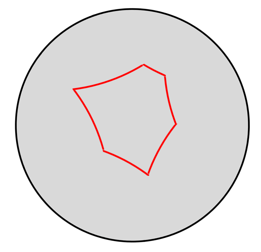
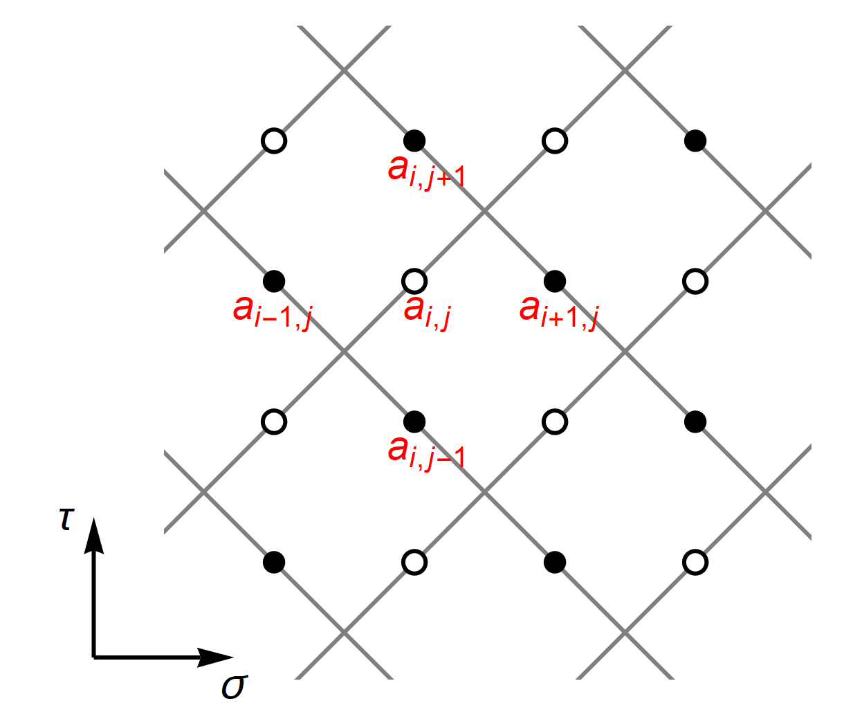
Figure 1: Left: Segmented string on a timeslice of global AdS₃. The individual segments are linear AdS₂ subspaces in ${\mathbb{{R}}}^{2,2}$. In the example there are six kinks moving with the speed of light. Right: The worldsheet of segmented strings. Kink worldlines form a rectangular lattice on the worldsheet. Their motion is characterized by constant null tangent vectors $X\in{\mathbb{{R}}}^{2,2}$ which only change when they collide with other kinks. The ‘celestial’ field $a={X_{-1}+X_{2}\over X_{0}+X_{1}}$ lives on the edges (indicated by black and white dots depending on edge orientation).

3 Segmented strings

The aim of this paper is to compute the spectral curve of strings in AdS₃. Instead of considering generic strings, we will restrict our attention to segmented strings which form a dense set in the space of all string solutions. Segmented strings are appropriate generalizations of piecewise linear strings in Minkowski spacetime: individual string segments are linear subspaces in ${\mathbb{{R}}}^{2,2}$ [31, 32]. For a closed string example on a timeslice of global AdS₃, see Figure 1 (left). The string in the example (red line) consists of six segments connected by kinks. Each of the segments have a constant normal vector. Kinks must move with the speed of light which implies that the scalar product of normal vectors of adjacent patches must be equal to one. Due to the Virasoro constraints (1), kinks also move on null lines on the worldsheet. Hence their worldlines form a rectangular lattice as seen in Figure 1 (right). Each diamond in the figure is a patch of AdS₂ with a constant normal vector. Whenever two kinks collide, a string segment vanishes. The collision results in a new segment with a different normal vector which can be computed by a reflection formula. Time evolution can also be obtained by an alternative reflection formula which computes the fourth kink collision spacetime point from the other three on any AdS₂ diamond on the woldsheet [31, 32, 33, 34, 35].

3.1 Celestial variables

In [33] I showed that segmented strings can be described by a discrete-time affine Toda model. Kink worldlines have constant null tangent vectors which can be decomposed into products of spinor pairs. The area of the worldsheet can be expressed in terms of these spinors which results in the equation of motion

$$\hskip-4.26773pt{1\over a_{ij}-a_{i,j+1}}+{1\over a_{ij}-a_{i,j-1}}={1\over a_{ij}-a_{i+1,j}}+{1\over a_{ij}-a_{i-1,j}}\,.$$ (12)

Here $i$ and $j$ are integer indices labeling kink worldlines as shown in Figure 1 (right). Black and white dots indicate the orientation of the edges. The field $a_{ij}\in{\mathbb{{R}}}$ is the celestial variable which can be computed by the formula

$${a}={X_{-1}+X_{2}\over X_{0}+X_{1}}\,,$$ (13)

where $X$ is the null tangent vector of the kink. Hence, this field lives on the edges on the kink lattice. Null vectors can be rescaled by a constant factor but this ambiguity drops out of the expression. The equation (12) is non-linear and produces interesting chaotic phenomena [27]. The Cauchy data can be given by specifying two rows of celestial variables, e.g. $a_{i,0}$ and $a_{i,1}$ for all $i$. The variables have to satisfy certain inequality constraints to make sure that the patch areas are non-negative. The string embedding can be obtained from the celestial variables up to a global $SL(2)$ isometry transformation [33].

In the continuum limit the discrete $a$ field becomes two separate real scalar fields: $b(z,\bar{z})$ and $w(z,\bar{z})$ named after the color of the dots. These fields are ${\mathbb{{R}}}^{2,2}$ analogs of coordinates on the celestial sphere which is the sphere at null infinity in Minkowski spacetime (see [36] and also [37] for the scattering problem in $(2,2)$ signature).

The celestial fields satisfy the equation of motion [25]

$$\partial\bar{}\partial b={2\partial b\bar{}\partial b\over b-w}\,,\qquad\partial\bar{}\partial w={2\partial w\bar{}\partial w\over w-b}\,,$$ (14)

which can be derived from either of the following actions

$$S_{1}=2\int{\bar{}\partial b\partial w\over(b-w)^{2}}dzd\bar{z}\,,\qquad S_{2}=2\int{\bar{}\partial w\partial b\over(b-w)^{2}}dzd\bar{z}\,.$$ (15)

Henceforth we will use $b$ and $w$ instead of $a$ to denote the celestial field even in the discrete case. The null tangent vector satisfies either $X\propto\partial Y$ or $X\propto\bar{}\partial Y$ depending on which way the kink moves. From (5) one can see that the celestial field can be computed by taking the ratio of the two elements in the first column. Therefore the $b$ and $w$ fields can be computed from the $W$ tensor (4) by [25]

$$b(z,\bar{z})={(\partial Y)_{-1}+(\partial Y)_{2}\over(\partial Y)_{0}+(\partial Y)_{1}}={\psi^{L}_{10}\psi^{R}_{\dot{0}\dot{0}}\over\psi^{L}_{11}\psi^{R}_{\dot{0}\dot{0}}}={\psi^{L}_{10}\over\psi^{L}_{11}}\,,$$ (16)

where the first (second) spinor index is the internal (spacetime) index. Similarly we have

$$w(z,\bar{z})={(\bar{}\partial Y)_{-1}+(\bar{}\partial Y)_{2}\over(\bar{}\partial Y)_{0}+(\bar{}\partial Y)_{1}}={\psi^{L}_{00}\over\psi^{L}_{01}}$$ (17)

Note that the formulas only depend on the spinors of the left system.

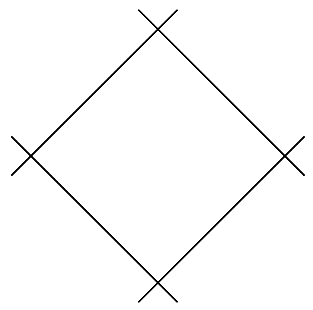
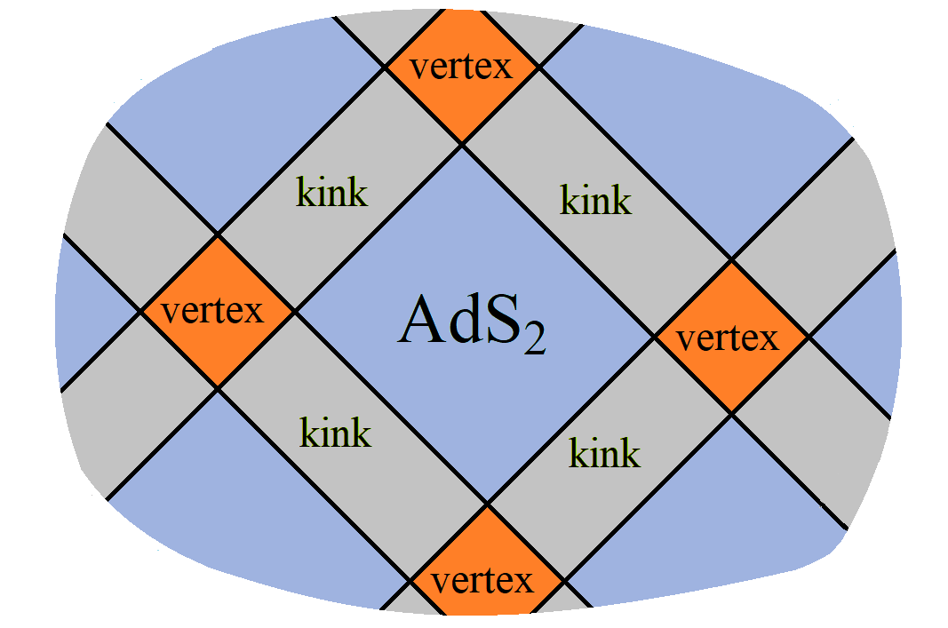
Figure 2: Left: The vicinity of an AdS₂ patch on the worldsheet. The patch is bounded by the worldlines of four kinks. Right: The same worldsheet patch with rescaled coordinates which blow up the vertex (orange) and kink (gray) regions. In the AdS₂ regions (blue), the normal vector is constant and the position vector changes. In the vertex regions, the position vector is constant and the normal vector changes continuously.

4 The scattering problem

In order to compute the Lax monodromy, we need to find solutions to the linear problem in eqn. (11). For segmented strings this will be facilitated by the fact that on different patches the equations simplify and explicit solutions can be found.

Figure 2 (left) shows the vicinity of an AdS₂ patch on the worldsheet. Black lines indicate kink worldlines. Inside the diamond the area density is equal to $2e^{2\alpha(z,\bar{z})}$ which is a finite quantity. On the other hand, $u$ and $v$ are vanishingly small and thus $\alpha$ satisfies the Liouville equation. At the kink collision vertices, $u$ and $v$ blow up. By a conformal transformation this divergence can be eliminated. The new coordinate system is shown in Figure 2 (right). The vertex regions are blown up into orange diamonds. In these regions the area density vanishes while the dual area density $\beta$ remains finite. It can be defined by

$$e^{2\beta(z,\bar{z})}={\frac{1}{2}}\partial N\cdot\bar{}\partial N\,,$$

where $N$ is the normal vector.

In the following, we will compute the spinor solutions in the vertex and AdS₂ regions and then we will match them in the overlap region.

4.1 AdS₂ patches

In AdS₂ regions we have $u=v=0$ and thus the Lax connection simplifies to

$$B_{z}=\begin{pmatrix}{1\over 2}\partial\alpha&{-{1\over\zeta}e^{{\alpha}}}\cr 0&-{1\over 2}\partial\alpha\end{pmatrix}\,,\quad B_{\bar{z}}=\begin{pmatrix}-{1\over 2}\bar{}\partial\alpha&0\cr-\zeta e^{{\alpha}}&{1\over 2}\bar{}\partial\alpha\end{pmatrix}\,,$$

and the generalized sinh-Gordon field solves the Liouville equation $\partial\bar{}\partial\alpha=e^{2\alpha}$. The solution can be expressed in terms of two arbitrary functions $f(z)$ and $g(\bar{z})$

$$e^{2\alpha}=-{f^{\prime}(z)g^{\prime}(\bar{z})\over[f(z)-g(\bar{z})]^{2}}\,.$$ (18)

Positivity of the area density requires $f^{\prime}(z)g^{\prime}(\bar{z})<0$. We further assume $f(z)<g(\bar{z})$. The solutions of the scattering problem in (11) can be written as

$$\psi_{\alpha a}=\left[g(\bar{z})-f(z)\right]^{-{1\over 2}}\begin{pmatrix}\quad\left[c^{1}_{a}+c^{0}_{a}f(z)\right]\zeta^{-{1\over 2}}\left(-{g^{\prime}(\bar{z})\over f^{\prime}(z)}\right)^{1\over 4}\cr-\left[c^{1}_{a}+c^{0}_{a}g(\bar{z})\right]\zeta^{{1\over 2}}\left(-{f^{\prime}(z)\over g^{\prime}(\bar{z})}\right)^{1\over 4}\end{pmatrix}\,.$$ (19)

where $a\in\{0,1\}$ labels the two linearly independent solutions, $\alpha\in\{0,1\}$ denotes the spinor index and $c^{i}_{a}$ are four arbitrary real constants. The solution is valid in the vicinity of an AdS₂ patch. In Figure 3 (right) the boundary of this region is indicated by a dashed line.

4.2 Kink collision vertices

There is a symmetry between AdS₂ and vertex regions with the area and dual area densities exchanged. Note that in a coordinate system where $u=v=\textrm{const.}$, a new solution to eq. (11) can be obtained by the transformation that simultaneously exchanges the following quantities:

$$\alpha\leftrightarrow\beta\,,\qquad z\leftrightarrow\bar{z}\,,\qquad\zeta\leftrightarrow\zeta^{-1}\,.$$

Hence, similarly to (18), we can write the dual area density as

$$e^{2\beta}=-{\tilde{f}^{\prime}(z)\tilde{g}^{\prime}(\bar{z})\over[\tilde{f}(z)-\tilde{g}(\bar{z})]^{2}}\,.$$ (20)

Let us parametrize the spinors solution in the vertex regions as

$$\tilde{\psi}_{\alpha a}=[\tilde{f}(z)-\tilde{g}(\bar{z})]^{-{1\over 2}}\begin{pmatrix}\left[\tilde{c}^{1}_{a}+\tilde{c}^{0}_{a}\tilde{g}(\bar{z})\right]\zeta^{1\over 2}\left(-{\tilde{f}^{\prime}(z)\over\tilde{g}^{\prime}(\bar{z})}\right)^{1\over 4}\cr-[\tilde{c}^{1}_{a}+\tilde{c}^{0}_{a}\tilde{f}(z)]\zeta^{-{1\over 2}}\left(-{\tilde{g}^{\prime}(\bar{z})\over\tilde{f}^{\prime}(z)}\right)^{1\over 4}\end{pmatrix}\,,$$ (21)

where tildes have been added to the various quantities to distinguish them from those appearing in (19). The solution is valid in the vicinity of a vertex patch. In Figure 3 (right) the boundary of this region is indicated by a dotted line.

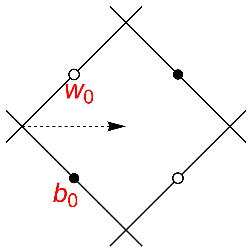
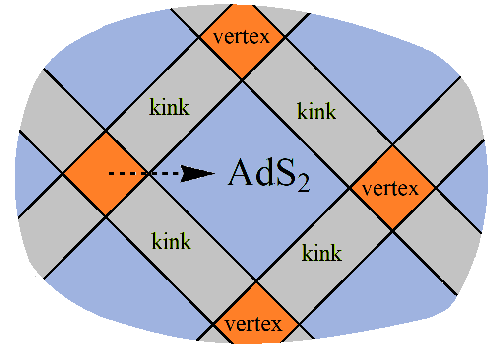
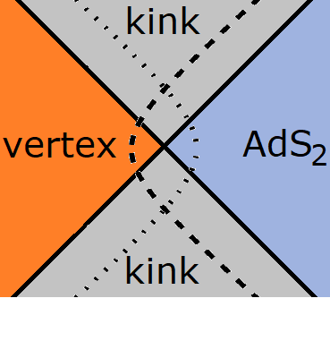
Figure 3: Left: The arrow indicates the path for which the connection matrix can be computed in terms of the $b_{0}$ and $w_{0}$ celestial fields. Middle: The same worldsheet patch after a conformal transformation. Right: The $\psi_{\alpha a}$ and $\tilde{\psi}_{\alpha a}$ solutions of the AdS₂ and vertex regions are valid to the right of the dashed line and to the left of the dotted line, respectively.

4.3 Local frame

In the following, we will specify the $f,\tilde{f},g,\tilde{g}$ functions, which amounts to choosing a local frame for the spinors. The global solution will then be determined by the $c^{i}_{a}$ and $\tilde{c}^{j}_{b}$ variables which can be thought of as piecewise constant functions on the union of AdS₂ and vertex patches, respectively. Note that the kink regions (gray areas in Figure 3 (middle)) play no role in the construction.

The spin frame will be defined using the $\zeta=1$ spinors solutions (see Appendix A in [30]). These are physical in the sense that they determine the string embedding via (9). Equations (16) and (17) define the physical celestial variables which can be used to fix $f,\tilde{f},g,\tilde{g}$. Generically $b=b(z,\bar{z})$ and $w=w(z,\bar{z})$. This is simplified in the vertex and AdS₂ regions of a segmented string: the celestial variables only depend on either $z$ or $\bar{z}$ [25]. Thus, we can set

$$f(z)=w(z)\,,\quad g(\bar{z})=b(\bar{z})\,,\quad c_{a}^{i}=\delta_{a}^{i}$$ (22)

on AdS₂ patches and

$$\tilde{f}(z)=b(z)\,,\quad\tilde{g}(\bar{z})=w(\bar{z})\,,\quad\tilde{c}_{a}^{i}=\delta_{a}^{i}$$ (23)

on vertex patches. Note that with this choice, the solutions are properly normalized according to (8). By plugging these functions into (18) and (20) one can see that they indeed give the correct area and dual area densities [25]

$$e^{2\alpha}=-{\bar{}\partial b\partial w\over(b-w)^{2}}\,,\qquad e^{2\beta}=-{\partial b\bar{}\partial w\over(b-w)^{2}}\,.$$

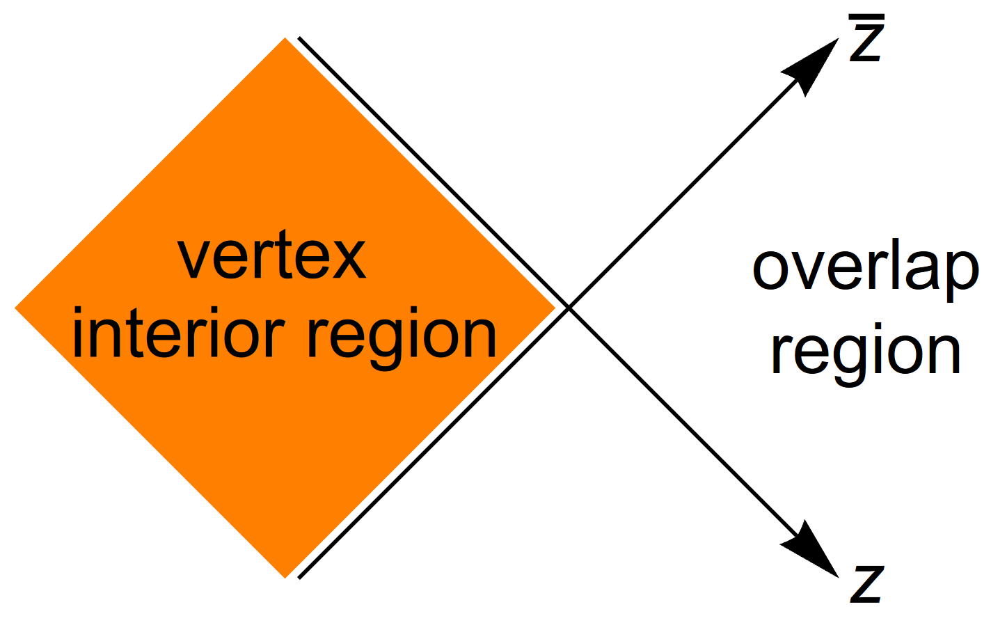
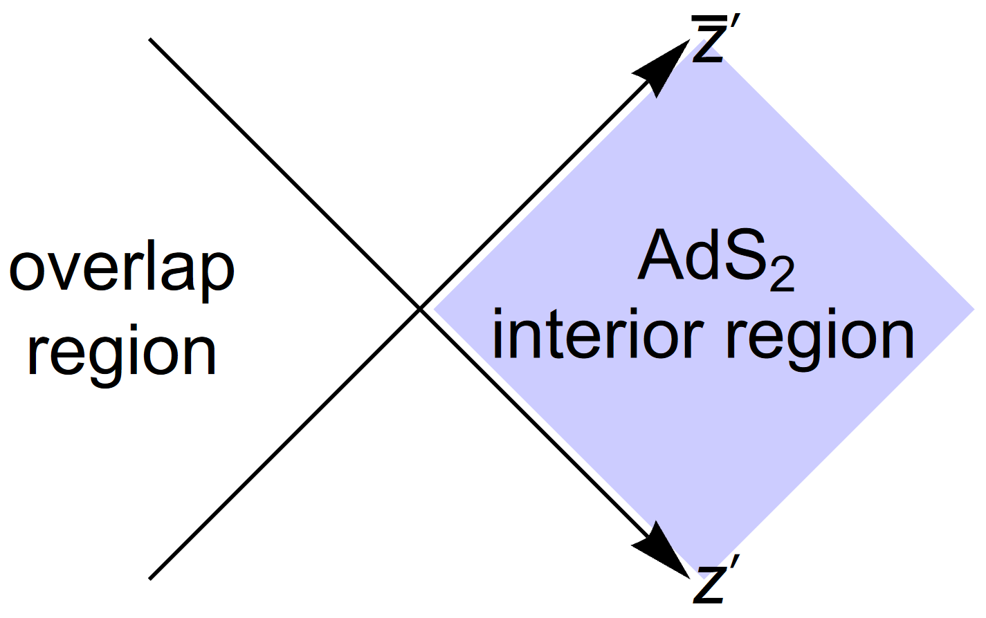
Figure 4: Coordinate systems for the matched asymptotic expansion.

4.4 Matching the solutions

The spinor solutions (19) and (21) are only valid strictly inside AdS₂ and vertex patches, respectively. In order to match them, we need to define them in slightly larger regions as seen in Figure 3 (right). This is still possible within the framework of the Liouville equation. Let us consider, for instance, a vertex patch. This patch, along with a small surrounding area on the worldsheet (to the left of the dotted line in the Figure) is mapped into the vicinity of a spacetime point. After zooming in, the target space curvature is scaled out and what is left is a piecewise linear string in Minkowski space satisfying the Liouville equation (see section 2 in [12]). Similarly, the Liouville equation is capable of describing AdS₂ patches with their infinitesimally small neighborhoods (everything to the right of the dashed line in Figure 3 (right)). In the intersection of the two regions, both non-linear terms in the sinh-Gordon equation vanish and thus we have $\partial\bar{}\partial\alpha=0$ (and similarly $\partial\bar{}\partial\beta=0$).

We would like to make sure that the solutions are correctly glued and that the spin frame is globally well-defined. This requires that in the overlap region

$$\psi_{\alpha,0}({\zeta=1})=\tilde{\psi}_{\alpha,0}({\zeta=1})\,\quad\textrm{and}\quad\psi_{\alpha,1}({\zeta=1})=\tilde{\psi}_{\alpha,1}({\zeta=1})\,.$$

Let us consider two separate coordinate systems $(z,\bar{z})$ and $(z^{\prime},\bar{z}^{\prime})$ for the vertex and AdS₂ patches, respectively. In the coordinate system for the vertex and AdS₂ patches the overlapping regions are assumed to lie in the quadrants $z,\bar{z}>0$ and $z^{\prime},\bar{z}^{\prime}<0$, respectively; see Figure 4. The opposite quadrants ($z,\bar{z}<0$ and $z^{\prime},\bar{z}^{\prime}>0$) are the interior regions of the patches: these are the orange and blue regions in Figure 3 (right). We choose the coordinates so that in the interior regions $b$ and $w$ are fractional linear functions (of the appropriate single variable), and the $f,\tilde{f},g,\tilde{g}$ functions are set equal to them according to (22) and (23).

In the overlapping regions, $f,\tilde{f},g,\tilde{g}$ should asymptote to constants

$$\lim_{z^{\prime}\to-\infty}f(z^{\prime})=\lim_{\bar{z}\to+\infty}\tilde{g}(\bar{z})=w_{0}\,,\qquad\lim_{z\to+\infty}\tilde{f}(z)=\lim_{\bar{z}^{\prime}\to-\infty}g(\bar{z}^{\prime})=b_{0}\,.$$

As a simple example let us consider the functions

$$f(z^{\prime})=w_{0}-\varepsilon\log(1+e^{z^{\prime}/\varepsilon})\,\qquad\textrm{and}\qquad g(\bar{z}^{\prime})=b_{0}+\varepsilon\log(1+e^{\bar{z}^{\prime}/\varepsilon})$$

which interpolate between $w_{0}$ and $w_{0}-z^{\prime}$ and between $b_{0}$ and $b_{0}+\bar{z}^{\prime}$, respectively. Here $\varepsilon$ is a small parameter. Similarly, consider

$$\tilde{f}(z)=b_{0}+\varepsilon\log(1+e^{-z/\varepsilon})\,\qquad\textrm{and}\qquad\tilde{g}(\bar{z})=w_{0}-\varepsilon\log(1+e^{-\bar{z}/\varepsilon})\,,$$

which interpolate between $b_{0}-z$ and $b_{0}$ and between $w_{0}+\bar{z}$ and $w_{0}$, respectively. The corresponding spinors (with $\zeta=1$) in the overlapping region are

$$\psi_{\alpha,0}\approx(b_{0}-w_{0})^{-{1\over 2}}\begin{pmatrix}w_{0}\,e^{{(\bar{z}^{\prime}-z^{\prime})/(4\varepsilon)}}\cr-b_{0}\,e^{{(z^{\prime}-\bar{z}^{\prime})/(4\varepsilon)}}\end{pmatrix}\,,\qquad\psi_{\alpha,1}\approx(b_{0}-w_{0})^{-{1\over 2}}\begin{pmatrix}e^{{(\bar{z}^{\prime}-z^{\prime})/(4\varepsilon)}}\cr-e^{{(z^{\prime}-\bar{z}^{\prime})/(4\varepsilon)}}\end{pmatrix}\,,$$

$$\tilde{\psi}_{\alpha,0}\approx(b_{0}-w_{0})^{-{1\over 2}}\begin{pmatrix}w_{0}\,e^{{(\bar{z}-z)/(4\varepsilon)}}\cr-b_{0}\,e^{{(z-\bar{z})/(4\varepsilon)}}\end{pmatrix}\,,\qquad\tilde{\psi}_{\alpha,1}\approx(b_{0}-w_{0})^{-{1\over 2}}\begin{pmatrix}e^{{(\bar{z}-z)/(4\varepsilon)}}\cr-e^{{(z-\bar{z})/(4\varepsilon)}}\end{pmatrix}\,.$$

Identifying $z-\bar{z}=z^{\prime}-\bar{z}^{\prime}$ we see that $\psi_{\alpha,0}=\tilde{\psi}_{\alpha,0}$ and $\psi_{\alpha,1}=\tilde{\psi}_{\alpha,1}$. Note that they are not constants, but their dependence on the coordinates are the same. The example can easily be generalized to interpolating functions connecting fractional linear functions to $b_{0}$ and $w_{0}$.

For $\zeta\neq 1$ the Lax connection matrix will generally be non-trivial. We can compute it by equating $\psi$ and $\tilde{\psi}$ in the overlapping region which defines the discrete Lax matrix $\Omega$

$$\psi_{\alpha a}=\Omega_{ab}(b_{0},w_{0},\zeta)\tilde{\psi}_{\alpha b}\,,\qquad\textrm{or}\qquad\psi=\tilde{\psi}\Omega^{T}\,,$$ (24)

where the spinors can be written as

$$\psi=(b_{0}-w_{0})^{-{\frac{1}{2}}}\begin{pmatrix}\left(-{g^{\prime}(\bar{z}^{\prime})\over f^{\prime}(z^{\prime})}\right)^{1\over 4}&0\cr 0&\left(-{f^{\prime}(z^{\prime})\over g^{\prime}(\bar{z}^{\prime})}\right)^{1\over 4}\end{pmatrix}\begin{pmatrix}\zeta^{-{\frac{1}{2}}}&0\cr 0&\zeta^{{\frac{1}{2}}}\end{pmatrix}\begin{pmatrix}w_{0}&1\cr-b_{0}&-1\end{pmatrix}\,,$$

$$\tilde{\psi}=(b_{0}-w_{0})^{-{\frac{1}{2}}}\begin{pmatrix}\left(-{\tilde{f}^{\prime}(z)\over\tilde{g}^{\prime}(\bar{z})}\right)^{1\over 4}&0\cr 0&\left(-{\tilde{g}^{\prime}(\bar{z})\over\tilde{f}^{\prime}(z)}\right)^{1\over 4}\end{pmatrix}\begin{pmatrix}\zeta^{{\frac{1}{2}}}&0\cr 0&\zeta^{-{\frac{1}{2}}}\end{pmatrix}\begin{pmatrix}w_{0}&1\cr-b_{0}&-1\end{pmatrix}\,.$$

As we have seen, in the overlap regions we have ${g^{\prime}(\bar{z}^{\prime})\over f^{\prime}(z^{\prime})}={\tilde{f}^{\prime}(z)\over\tilde{g}^{\prime}(\bar{z})}$. Thus, (24) simplifies to

$$\begin{pmatrix}\zeta^{-{\frac{1}{2}}}&0\cr 0&\zeta^{{\frac{1}{2}}}\end{pmatrix}\begin{pmatrix}w_{0}&1\cr-b_{0}&-1\end{pmatrix}=\begin{pmatrix}\zeta^{{\frac{1}{2}}}&0\cr 0&\zeta^{-{\frac{1}{2}}}\end{pmatrix}\begin{pmatrix}w_{0}&1\cr-b_{0}&-1\end{pmatrix}\Omega^{T}\,.$$

This is solved by

$$\Omega_{b_{0},w_{0}}={1\over(b_{0}-w_{0})\zeta}\begin{pmatrix}{b_{0}\zeta^{2}-w_{0}}&{b_{0}w_{0}(1-\zeta^{2})}\cr{\zeta^{2}-1}&{b_{0}-w_{0}\zeta^{2}}\end{pmatrix}\,,$$

where we have adopted the notation that the celestial fields are written as a subscript (not to be confused with the spacetime spinor indices in (24)).

5 The discrete Lax matrix

In the previous section we have computed the connection matrix for a path that started on an AdS₂ patch and ended on an adjacent vertex (see dashed line in Figure 3 (left)). The result depends on the two nearest celestial variables

$$\Omega_{b,w}(\zeta)={1\over(b-w)\zeta}\begin{pmatrix}{b\zeta^{2}-w}&{bw(1-\zeta^{2})}\cr{\zeta^{2}-1}&{b-w\zeta^{2}}\end{pmatrix}$$ (25)

The Lax matrix is in $SL(2,{\mathbb{{R}}})$

$$\det\Omega_{b,w}=1\,,$$

and without the spectral parameter it is equal to the $2\times 2$ identity matrix by construction

$$\Omega_{b,w}(\zeta=1)=\mathbb{1}\,.$$

Although in the example in Figure 3 the path goes ‘east’, (25) gives the connection matrix for the other three directions as well. Note that the path is always pointing from the vertex to the inside of the AdS₂ patch. The Lax matrix of the reverse path is given by

$$\Omega_{b,w}^{-1}(\zeta)=\Omega_{w,b}(\zeta)=\Omega_{b,w}(\zeta^{-1})\,.$$

Simultaneous Möbius transformations of the celestial variables

$$b\to b^{\prime}={a_{00}b+a_{01}\over a_{10}b+a_{11}}\,,\qquad w\to w^{\prime}={a_{00}w+a_{01}\over a_{10}w+a_{11}}$$

are isometry transformations of AdS₃. The connection matrix transforms covariantly

$$\Omega_{b,w}\to U\Omega_{b^{\prime},w^{\prime}}U^{-1}\,\qquad\textrm{with}\qquad U=\begin{pmatrix}a_{00}&a_{01}\cr a_{10}&a_{11}\end{pmatrix}\,.$$

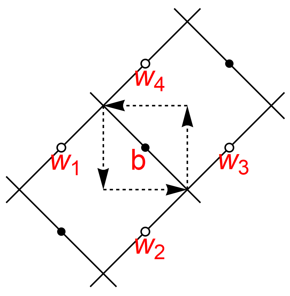
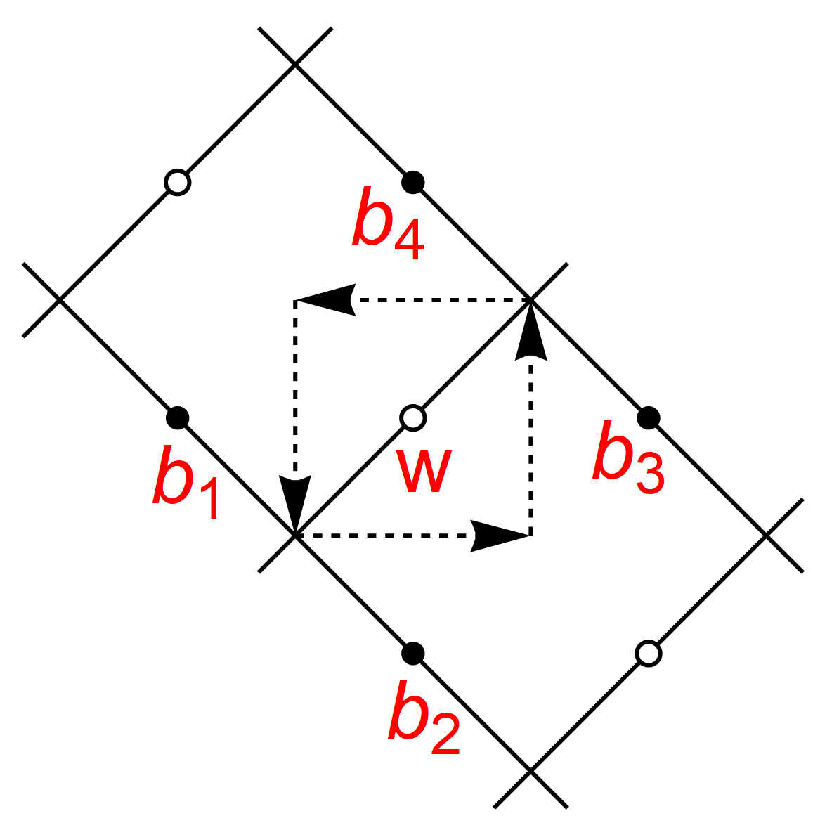
Figure 5: Monodromy around trivial loops. The (12) equation of motion relates $b$ and the four $w_{i}$ variables (and similarly $w$ and the four $b_{i}$) ensuring the flatness of the connection.

5.1 Flatness

The connection is flat and thus it is trivial around contractible loops. We will first show this for the smallest loops which consist of four elementary paths as in Figure 5. Assuming the $b$, $w_{1},w_{2},w_{3},w_{4}$ celestial variables satisfy the equation of motion in (12), i.e.

$${1\over b-w_{2}}+{1\over b-w_{4}}={1\over b-w_{1}}+{1\over b-w_{3}}\,,$$

we get

$$\Omega_{b,w_{4}}^{-1}\Omega_{b,w_{3}}\Omega_{b,w_{2}}^{-1}\Omega_{b,w_{1}}=\mathbb{1}\,$$

for any $\zeta$. The monodromy around a white dot also gives a similar trivial result,

$$\Omega_{b_{4},w}\Omega_{b_{3},w}^{-1}\Omega_{b_{2},w}\Omega_{b_{1},w}^{-1}=\mathbb{1}\,,$$

if the equation of motion is used again. Larger contractible loops can be built from the two small loops. Hence the monodromy for all of these will be trivial.

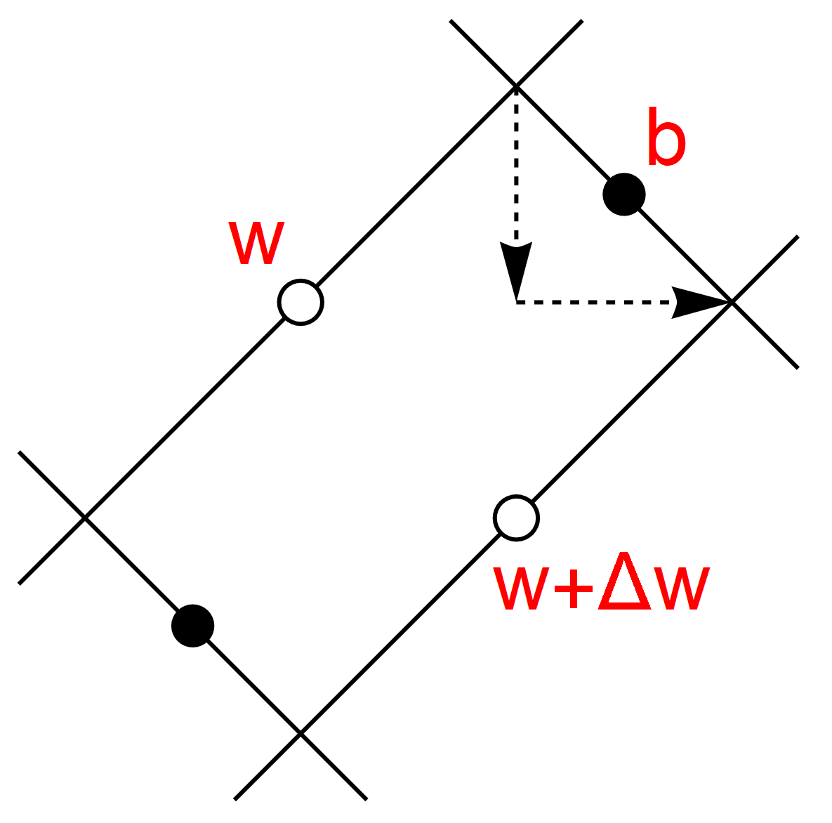
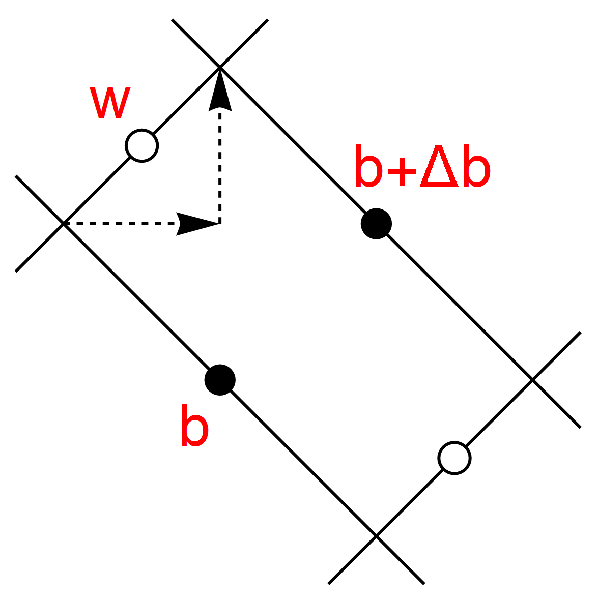
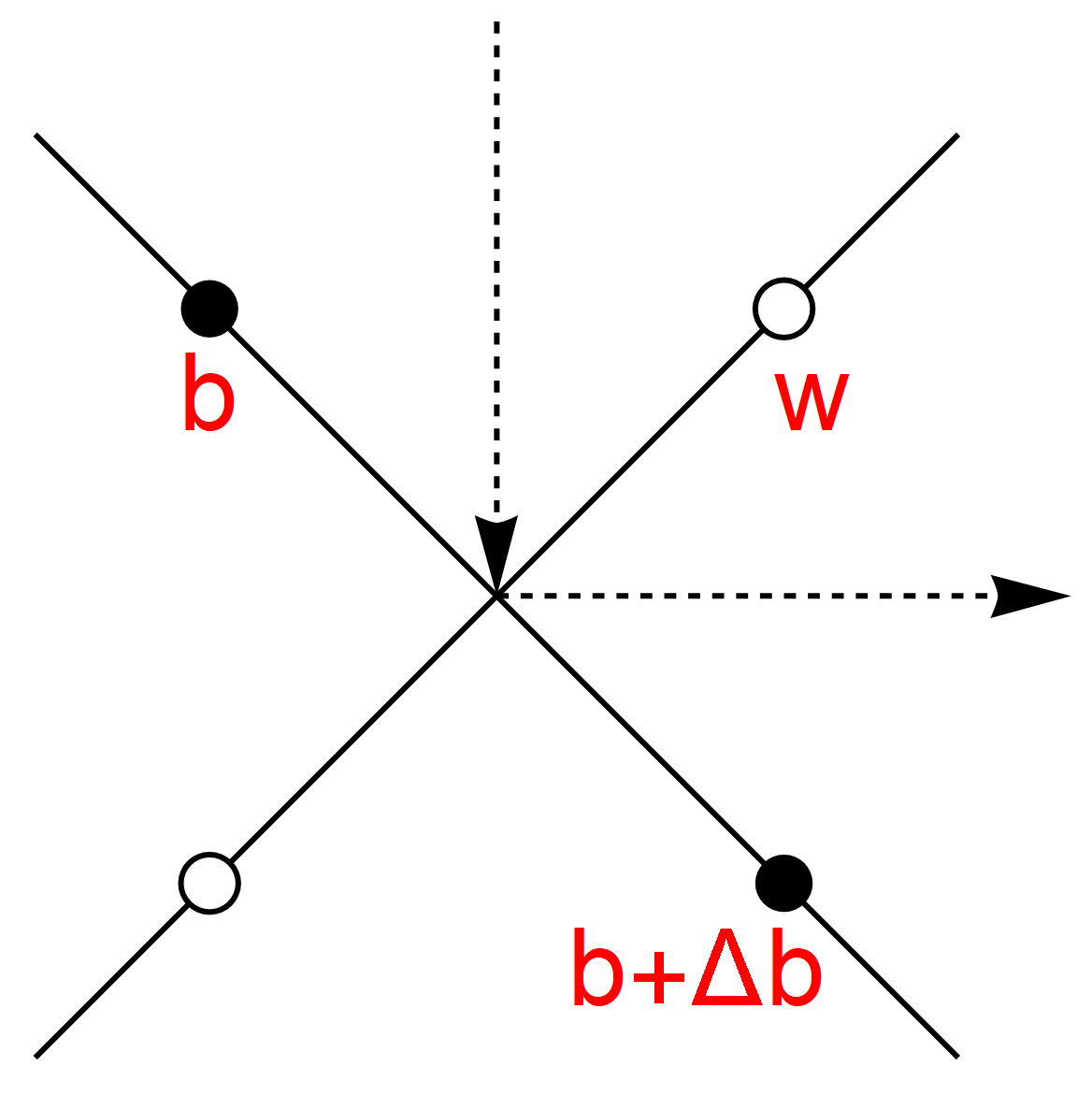
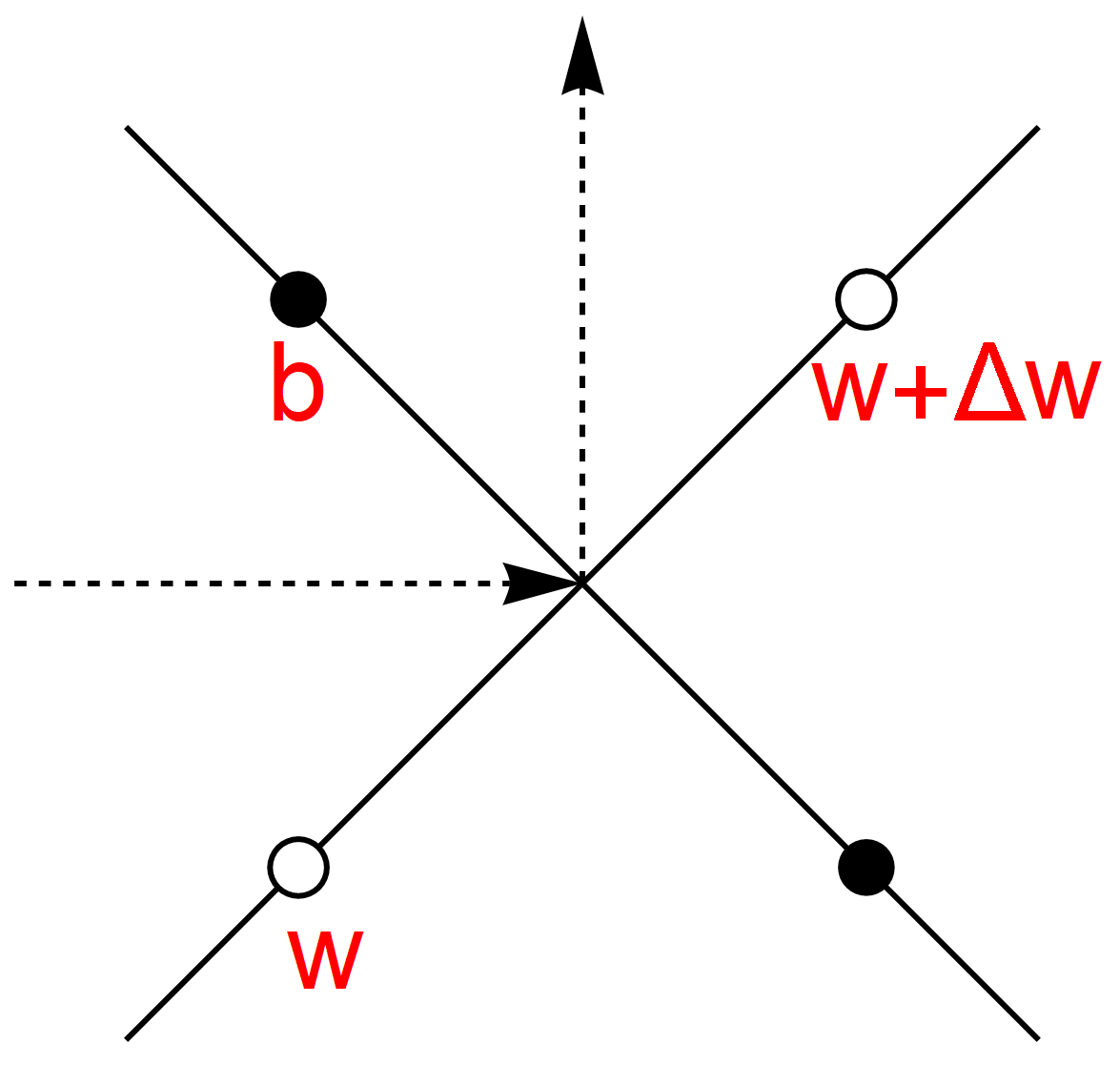
Figure 6: Taking the continuum limit of the discrete Lax matrix.

5.2 Continuum limit

Taking the continuum limit of $\Omega_{b,w}$ is not immediately possible, because the matrix depends on two variables $b$ and $w$ that are only equal when the string touches the AdS boundary. One can, however, take the product of two Lax matrices as shown in the first two diagrams in Figure 6. For small $\Delta w\approx\partial w\,\Delta z$ we have

$$\Omega^{-1}_{b,w+\Delta w}\Omega_{b,w}\approx\mathbb{1}+{j_{z}\over 1-x}\Delta z\,,\qquad j_{z}={2\over(b-w)^{2}}\begin{pmatrix}-b\partial w&b^{2}\partial w\cr-\partial w&b\partial w\end{pmatrix}\,,$$ (26)

and similarly in the $\bar{z}$ direction (with $\Delta b\approx\bar{}\partial b\,\Delta\bar{z}$)

$$\Omega^{-1}_{b+\Delta b,w}\Omega_{b,w}\approx\mathbb{1}+{j_{\bar{z}}\over 1+x}\Delta\bar{z}\,,\qquad j_{\bar{z}}={2\over(b-w)^{2}}\begin{pmatrix}-w\bar{}\partial b&w^{2}\bar{}\partial b\cr-\bar{}\partial b&w\bar{}\partial b\end{pmatrix}\,.$$ (27)

Here we have introduced a new spectral parameter $x$, which usually appears in the definition of the Lax connection of the principal chiral model. It is related to $\zeta$ by

$$\zeta=\sqrt{x-1\over x+1}\,.$$ (28)

Another pair of matrices can be obtained from the paths that start and end on adjacent AdS₂ patches; see the diagrams on the RHS of Figure 6. From these paths we get

$$\Omega_{b+\Delta b,w}\Omega^{-1}_{b,w}\approx\mathbb{1}+{\tilde{\jmath}_{z}\over 1-x}\Delta z\,,\qquad\tilde{\jmath}_{z}={2\over(b-w)^{2}}\begin{pmatrix}-w\partial b&w^{2}\partial b\cr-\partial b&w\partial b\end{pmatrix}\,,$$

$$\Omega_{b,w+\Delta w}\Omega^{-1}_{b,w}\approx\mathbb{1}+{\tilde{\jmath}_{\bar{z}}\over 1+x}\Delta\bar{z}\,,\qquad\tilde{\jmath}_{\bar{z}}={2\over(b-w)^{2}}\begin{pmatrix}-b\bar{}\partial w&b^{2}\bar{}\partial w\cr-\bar{}\partial w&b\bar{}\partial w\end{pmatrix}\,.$$

which are the same as (26), (27) with $b$ and $w$ exchanged.

Spacetime isometries act as Möbius transformations on the celestial variables. The two classically equivalent actions in (15) are invariant under such transformations and $j$ and $\tilde{\jmath}$ are the associated $SL(2)$ currents. They satisfy the conservation laws and flatness conditions

$$\partial j_{\bar{z}}+\bar{\partial}j_{z}=0\,,\qquad\partial\tilde{\jmath}_{\bar{z}}+\bar{\partial}\tilde{\jmath}_{z}=0\,,$$

$$\partial j_{\bar{z}}-\bar{\partial}j_{z}-[j_{z},j_{\bar{z}}]=0\,,\qquad\partial\tilde{\jmath}_{\bar{z}}-\bar{\partial}\tilde{\jmath}_{z}-[\tilde{\jmath}_{z},\tilde{\jmath}_{\bar{z}}]=0\,.$$

The currents can be written in the usual form $j=-dYY^{-1}$ where $Y_{a\dot{a}}$ is the embedding matrix in (5). For convenience, we repeat the discussion from Appendix A in [30]. If we define the matrices

$$M_{1}^{\alpha\dot{\beta}}=\begin{pmatrix}1&0\cr 0&1\end{pmatrix}\,,\qquad M_{2}^{\alpha\dot{\beta}}=\begin{pmatrix}0&1\cr 0&0\end{pmatrix}\,,\qquad M_{3}^{\alpha\dot{\beta}}=\begin{pmatrix}0&0\cr 1&0\end{pmatrix}\,,\qquad$$

then we have from (4)

$$Y_{a\dot{a}} = \psi^{L}_{\alpha a}M_{1}^{\alpha\dot{\beta}}\psi^{R}_{\dot{\beta}\dot{a}}=\left[(\psi^{L})^{t}M_{1}\psi^{R}\right]_{a\dot{a}}\,,$$

$$Y^{-1} = (\psi^{R})^{-1}M_{1}^{-1}\left[(\psi^{L})^{t}\right]^{-1}\,,$$

$$\partial Y = 2e^{\alpha}(\psi^{L})^{t}M_{3}\psi^{R}\,,$$

$$\bar{}\partial Y = 2e^{\alpha}(\psi^{L})^{t}M_{2}\psi^{R}\,.$$

Using these expressions, the left current can be written as

$${(j_{z})_{a}}^{b}=-\partial YY^{-1}=-2e^{\alpha}(\psi^{L})^{t}M_{3}M_{1}^{-1}\left[(\psi^{L})^{t}\right]^{-1}\,.$$

If we now plug in

$$\psi^{L}=(b-w)^{-{\frac{1}{2}}}\begin{pmatrix}w\left(-{\bar{}\partial b\over\partial w}\right)^{{1\over 4}}&\left(-{\bar{}\partial b\over\partial w}\right)^{{1\over 4}}\cr-b\left(-{\partial w\over\bar{}\partial b}\right)^{{1\over 4}}&-\left(-{\partial w\over\bar{}\partial b}\right)^{{1\over 4}}\end{pmatrix}\,,\qquad e^{\alpha}={\sqrt{-\bar{}\partial b\partial w}\over b-w}\,,$$

then we obtain precisely (26). Similarly we have

$${(j_{\bar{z}})_{a}}^{b}=-\bar{}\partial YY^{-1}=-2e^{\alpha}(\psi^{L})^{t}M_{2}M_{1}^{-1}\left[(\psi^{L})^{t}\right]^{-1}\,,$$

which gives the matrix in (27).

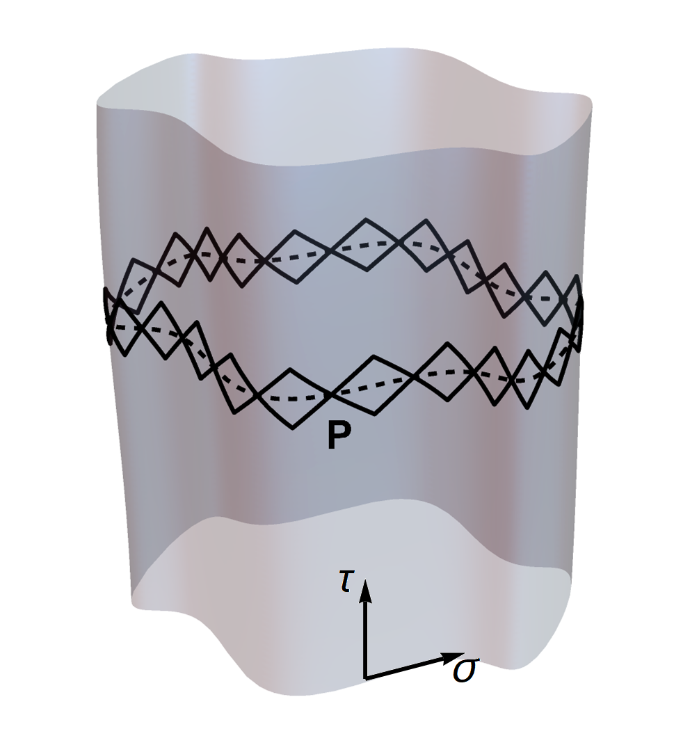
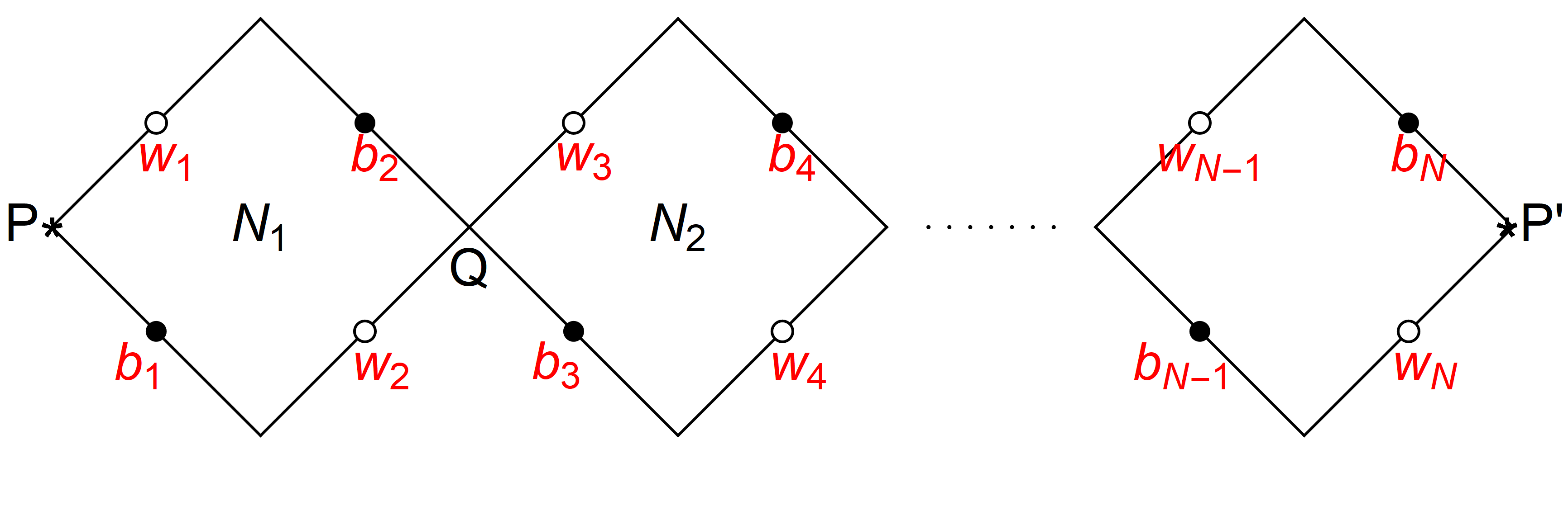
Figure 7: Left: Schematic drawing of the worldsheet of a closed string with $N$ segments. Kink worldlines are indicated near a timeslice (dashed loop). Right: Computing the monodromy around a closed loop. $P,Q,P^{\prime}\in{\mathbb{{R}}}^{2,2}$ denote kink collision vertices (we assume $P=P^{\prime}$). $N_{1}$ and $N_{2}$ are the normal vectors of the first two AdS₂ patches.

6 The monodromy

The spectral curve is obtained by computing the monodromy of the Lax connection around the non-trivial loop on the string worldsheet. This path and nearby kink worldlines are shown in Figure 7. Let us assume that on a generic time-slice there are an even number of string segments with ${N/2}$ left-moving and ${N/2}$ right-moving kinks. Then, the monodromy is a product of Lax matrices from $P$ to $P^{\prime}$ given by

$$\Omega(\zeta)=\Omega_{b_{N},w_{N}}^{-1}\Omega_{b_{N-1},w_{N-1}}\cdots\Omega_{b_{2},w_{2}}^{-1}\Omega_{b_{1},w_{1}}\,.$$ (29)

This formula gives an explicit expression for the monodromy in terms of the celestial variables associated with the kink velocities. Note that the monodromy depends on the starting point $P$ on the worldsheet. If this point is changed to $\tilde{P}$, then $\Omega$ changes by conjugation,

$$\Omega_{P}\to\Omega_{\tilde{P}}=U\Omega_{P}U^{-1}$$

where $U$ is the Lax matrix connecting $P$ and $\tilde{P}$.

6.1 Closing the string

For generic values of the $b_{1},w_{1},\ldots,b_{N},w_{N}$ celestial variables the string does not close. In the following we will compute $P^{\prime}$ from $P$ (both are considered to be points in ${\mathbb{{R}}}^{2,2}$) by a series of transformations and constrain the celestial variables by requiring $P=P^{\prime}$. First we compute the nearest normal vector

$$N_{1}=\mathcal{R}_{b_{1},w_{1}}P$$

where the ‘reflection matrix’ is given by [25]

$$\mathcal{R}_{b,w}={1\over b-w}\begin{pmatrix}0&bw+1&bw-1&-b-w\cr-1-bw&0&b+w&bw-1\cr-1+bw&b+w&0&-1-bw\cr-b-w&bw-1&bw+1&0\end{pmatrix}\,.$$ (30)

From $N_{1}$ we can compute the next vertex $Q$ via

$$Q=\mathcal{R}_{b_{2},w_{2}}N_{1}\,.$$

From $Q$ we compute $N_{2}$ and so on until we get to $P^{\prime}$. The final result contains the product of matrices

$$\mathcal{R}=\mathcal{R}_{b_{N},w_{N}}\cdots\mathcal{R}_{b_{2},w_{2}}\mathcal{R}_{b_{1},w_{1}}\,.$$ (31)

If $\mathcal{R}=\textrm{Id}_{4\times 4}$ then we have $P=P^{\prime}$. It turns out that this product can be repackaged into a product of $\Omega_{b,w}$ matrices as follows. Let us consider the $n^{\textrm{th}}$ matrix in the product. It can be decomposed as

$$\mathcal{R}_{b_{n},w_{n}}=c^{\mu}_{n}\Sigma_{\mu}\,,$$

where summation over $\mu\in\{0,1,2,3\}$ is understood. The constants are given by

$$c^{0}_{n}=0\,,\quad c^{1}_{n}={1-b_{n}w_{n}\over b_{n}-w_{n}}\,,\quad c^{2}_{n}=i{1+b_{n}w_{n}\over w_{n}-b_{n}}\,,\quad c^{3}_{n}={b_{n}+w_{n}\over w_{n}-b_{n}}\,,$$

and the $\Sigma_{\mu}$ are defined by

$$\Sigma_{0}=\mathbb{1}_{4\times 4}\,,\quad\Sigma_{1}=\begin{pmatrix}0&0&\hskip-5.69046pt-1&0\cr 0&0&0&\hskip-5.69046pt\hskip 0.0pt-1\cr-1&0&0&0\cr 0&\hskip-5.69046pt-1&0&0\end{pmatrix}\,,\quad\Sigma_{2}=\begin{pmatrix}0&i&0&0\cr-i&0&0&0\cr 0&0&0&-i\cr 0&0&i&0\end{pmatrix}\,,\quad\Sigma_{3}=\begin{pmatrix}0&0&0&1\cr 0&0&\hskip-5.69046pt-1&0\cr 0&\hskip-5.69046pt-1&0&0\cr 1&0&0&0\end{pmatrix}\,.$$

Since the matrices satisfy

$$\Sigma_{i}\Sigma_{j}=\delta_{ij}\Sigma_{0}+i\varepsilon_{ijk}\Sigma_{k}\,,$$

they generate an algebra isomorphic to the one generated by $\sigma_{0}=\mathbb{1}$ and the three $\sigma_{i}$ Pauli matrices. We can thus replace the $\Sigma$ matrices in $\mathcal{R}$ with their $2\times 2$ counterparts and define

$$\mathcal{R}^{\prime}=\prod_{n=N}^{1}c^{\mu}_{n}\sigma_{\mu}\,.$$

We have $\mathcal{R}^{\prime}=\mathbb{1}$ precisely when $\mathcal{R}=\Sigma_{0}$. As it happens, $\mathcal{R}^{\prime}$ can be rewritten in terms of the Lax matrices. For odd $n$ we have

$$c^{\mu}_{n}\sigma_{\mu}=i\sigma_{3}\Omega_{b_{n},w_{n}}(\zeta=i)\sigma_{3}\,,$$

and for even $n$ we write instead the equivalent expression

$$c^{\mu}_{n}\sigma_{\mu}=-i\sigma_{3}\Omega^{-1}_{b_{n},w_{n}}(\zeta=i)\sigma_{3}\,.$$

The $\sigma_{3}$ matrices and the constant $\pm i$ factors cancel in $\mathcal{R}^{\prime}$, which then gives the Lax monodromy from $P$ to $P^{\prime}$ (sandwiched between two $\sigma_{3}$ matrices). Thus, the string closes precisely when the monodromy at $\zeta=i$ (or $x=0$) is trivial, i.e.

$$\Omega(x=0)=\mathbb{1}\,.$$

Notice that the Lax matrix can be written as

$$\Omega_{b_{2},w_{2}}^{-1}(x=0)\Omega_{b_{1},w_{1}}(x=0)=QP^{-1}$$

and similarly for the other patches. Thus the monodromy can be written as

$$\Omega(x=0)=Y(2\pi)\,Y^{-1}(0)$$

where $Y(\sigma)\in SL(2,{\mathbb{{R}}})$ is the embedding function on a timeslice; see (5). If it is periodic, then $\Omega(x=0)$ is trivial. This criterion generally gives three real constraint equations for the celestial variables.

Recall that for $x=\infty$ or $0$ ($\zeta=1$ or $i$) the Lax connection yields the left and right connections, respectively, as seen in (10). In the first case we trivially have

$$\Omega(x=\infty)=\mathbb{1}\,,$$

since $\Omega_{b,w}(x=\infty)=\mathbb{1}$ for any values of $b$ and $w$.

6.2 The spectral curve

The quasimomentum $p(\zeta)$ is defined by

$$\cos p(\zeta)={\frac{1}{2}}\mathop{\rm tr}\Omega(\zeta)$$ (32)

Since the connection is flat, the result will only depend on $\zeta$ and the homotopy class of the loop. Since the celestial variables are real, for $\zeta\in{\mathbb{{R}}}$ we have $\cos p\in{\mathbb{{R}}}$ with forbidden zones located in the intervals where $|\cos p|>1$. Finally, the spectral curve is defined by the equation

$$\det(\lambda I-\Omega(\zeta))=0$$

in the space parametrized by $\{\lambda,\zeta\}\in{\mathbb{{C}}}^{2}$. It is more convenient to consider the algebraic curve associated to $p^{\prime}(x)$ which we write as

$$p^{\prime}(x)=-{{d\over dx}\cos p(x)\over\sqrt{1-\cos^{2}p(x)}}\,.$$

Taking the derivative gets rid of the $2\pi n$ phase shift ambiguity in $p$ and the resulting function can be made single-valued on two Riemann sheets. Properties of this curve can be inferred from the quasimomentum which is known explicitly in terms of the celestial variables via (32).

Let us consider a closed string of $N$ segments as in Figure 7. By inspecting the Lax matrices (25) written in terms of $x$

$$\Omega_{b,w}(x)={x\mathbb{1}+\Omega^{(0)}_{b,w}\over\sqrt{x^{2}-1}}\,\qquad\textrm{where}\qquad\Omega^{(0)}_{b,w}=\begin{pmatrix}-{b+w\over b-w}&{2bw\over b-w}\cr-{2\over b-w}&{b+w\over b-w}\end{pmatrix}\,,$$

it is easy to see that the quasimomentum takes the form

$$\cos p(x)={Q_{N}(x)\over(x^{2}-1)^{N\over 2}}\,,$$

where $Q_{N}$ is a degree $N$ polynomial in $x$ and is a function of the celestial variables $b_{i},w_{j}$ with $i,j=1,\ldots,N$. The coefficients of the polynomial are conserved charges. Using

$$\lim_{x\to\infty}\cos p(x)=1\,,$$

and $\mathop{\rm tr}\Omega^{(0)}_{b,w}=0$, it can also be shown that

$${d\over dx}\cos p(x)={P_{N-1}(x)\over(x^{2}-1)^{{N\over 2}+1}}\,,$$

and

$$1-\cos^{2}p(x)={Q_{2N-2}(x)\over(x^{2}-1)^{N}}\,,$$

where $P_{N-1}$ and $Q_{2N-2}$ are degree $N-1$ and $2N-2$ polynomials, respectively. The spectral curve can then be written as an algebraic curve,

$$p^{\prime}(x)=\pm{P_{N-1}(x)\over(x^{2}-1)\sqrt{Q_{2N-2}(x)}}$$

The function can be made single-valued on the hyperelliptic curve defined by $y^{2}=Q_{2N-2}(x)$. If there is a common factor in $P^{2}$ and $Q$, then the genus of the curve will be smaller than the naive expectation $g=N-2$. Since the Riemann surface has a finite genus, segmented strings are finite-gap solutions.

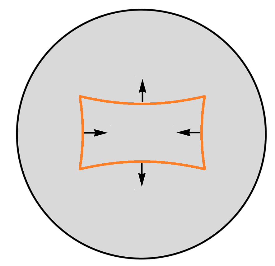
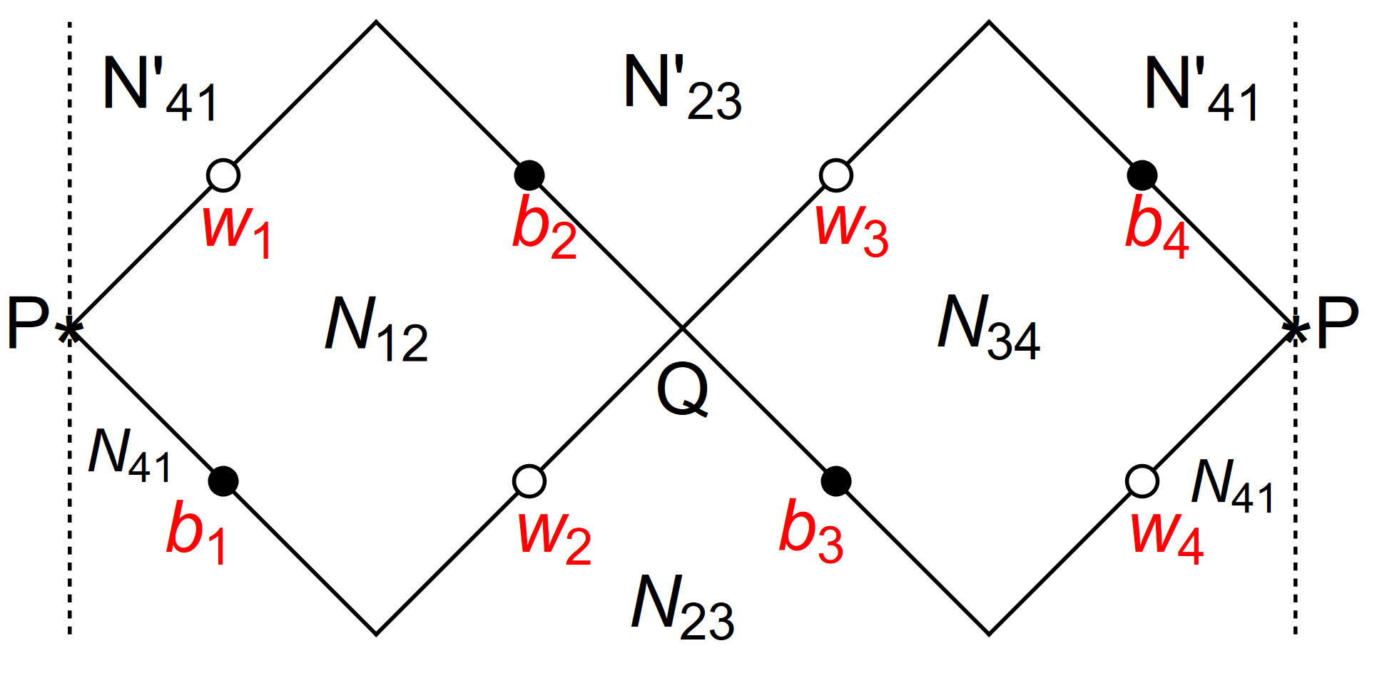
Figure 8: Left: Segmented string with four kinks on a timeslice of global AdS₃. In the applied coordinate system the segments are circular arcs. Arrows indicate the direction of motion of the segments. See [39] for an animation made by the authors of [32]. Right: A part of the worldsheet which should be glued along the dashed lines. $N_{12},N_{23},N^{\prime}_{23},N_{34},N_{41},N^{\prime}_{41}$ label the normal vectors of the corresponding AdS₂ patches. $b_{i}$ and $w_{j}$ are celestial variables. $P$ and $Q$ are spacetime points.

7 An example with four segments

In this section, as an example, we compute the spectral curve of a closed string with four segments. The motion of the string has been described in [32] (see [39] for an animation made by the authors). The string is seen in Figure 8 (left). It is a highest-weight (or primary) state which means that in our global AdS₃ coordinate system the ‘center-of-mass’ does not oscillate. After a while neighboring kinks collide and the segments start to move in the opposite direction. The worldsheet with the null kink worldlines are depicted in Figure 8 (right).

Initial conditions for the kinks were given in [32]. Let us label them by $i=1,\ldots,4$. Their initial position is given by

$$h_{i}=\left(\sqrt{1+r^{2}},\,0,\,r\cos\left((i-1){\pi\over 2}+\phi\right),\,r\sin\left((i-1){\pi\over 2}+\phi\right)\right)\in{\mathbb{{R}}}^{2,2}\,,$$

and their velocities are

$$v_{i}=\left(0,\,1,\,(-1)^{i+1}\sin\left((i-1){\pi\over 2}+\phi\right),\,(-1)^{i}\sin\left((i-1){\pi\over 2}+\phi\right)\right)\in{\mathbb{{R}}}^{2,2}\,.$$

Here $r$ determines the size of the oscillating string and $\phi$ is an offset angle corresponding to rotations in AdS₃. Note that $h_{i}^{2}=-1$ and $v_{i}^{2}=h_{i}v_{i}=0$ for $i=1,\ldots,4$.

In order to compute the spectral curve, one needs to obtain the celestial variables $b_{i}$ and $w_{j}$ corresponding to the kink velocities. $v_{i}$ correspond to the variables $b_{1},w_{2},b_{3},w_{4}$ which are given by (13),

$$b_{1}=-{\cos\phi\over 1+\sin\phi}\,,\quad w_{2}=-\cot{\phi\over 2}\,,\quad b_{3}={\cos\phi\over 1-\sin\phi}\,,\quad w_{4}=\tan{\phi\over 2}\,.$$

The easiest way to calculate the remaining celestial variables is to first compute the normal vectors. These are unit vectors perpendicular to both the positions of adjacent kinks and their velocities. For instance, we have

$$N_{12}^{2}=1,\,\quad N_{12}\cdot h_{1}=0,\,\quad N_{12}\cdot h_{2}=0,\,\quad N_{12}\cdot v_{1}=0,\,$$

which determines the four components of $N_{12}$ up to an overall sign. We obtain the expressions

$$N_{12} = \left(r,\,-\sqrt{1+r^{2}},\,\sqrt{1+r^{2}}(\cos\phi-\sin\phi),\,\sqrt{1+r^{2}}(\cos\phi+\sin\phi)\right)\,,$$

$$N_{23} = \left(r,\,\sqrt{1+r^{2}},\,-\sqrt{1+r^{2}}(\cos\phi+\sin\phi),\,\sqrt{1+r^{2}}(\cos\phi-\sin\phi)\right)\,,$$

$$N_{34} = \left(r,\,-\sqrt{1+r^{2}},\,\sqrt{1+r^{2}}(\sin\phi-\cos\phi),\,-\sqrt{1+r^{2}}(\cos\phi+\sin\phi)\right)\,,$$

$$N_{41} = \left(r,\,\sqrt{1+r^{2}},\,\sqrt{1+r^{2}}(\cos\phi+\sin\phi),\,\sqrt{1+r^{2}}(\sin\phi-\cos\phi)\right)\,.$$

Here we have fixed the signs of the normal vectors by demanding that the scalar product of adjacent vectors gives plus one. (There is still an overall sign ambiguity, which does not change the results.) Then, $N^{\prime}_{23}$ and $N^{\prime}_{41}$ can be computed from the reflection formula [31],

$$\hskip-22.76228ptN^{\prime}_{23}=-N_{23}+2{N_{12}+N_{34}\over 1+N_{12}\cdot N_{34}}=\sqrt{1+r^{2}}\left(-{r(3+2r^{2})\over(1+2r^{2})\sqrt{1+r^{2}}},\,{(1-2r^{2})\over 1+2r^{2}},\,\sin\phi+\cos\phi,\,\sin\phi-\cos\phi\right)\,,$$

$$\hskip-22.76228ptN_{41}=-N_{41}+2{N_{12}+N_{34}\over 1+N_{12}\cdot N_{34}}=\sqrt{1+r^{2}}\left(-{r(3+2r^{2})\over(1+2r^{2})\sqrt{1+r^{2}}},\,{(1-2r^{2})\over 1+2r^{2}},\,-\sin\phi-\cos\phi,\,\cos\phi-\sin\phi\right)\,.$$

Now the points $P$ and $Q$ can be determined using the reflection matrix (30),

$$P = \mathcal{R}_{b_{1},w_{4}}N_{41}=\left(\sqrt{1+r^{2}},\,r,\,r(\cos\phi+\sin\phi),\,r(\sin\phi-\cos\phi)\right)\,,$$

$$Q = \mathcal{R}_{b_{3},w_{2}}N_{23}=\left(\sqrt{1+r^{2}},\,r,\,-r(\cos\phi+\sin\phi),\,r(\cos\phi-\sin\phi)\right)\,.$$

The missing celestial variables $w_{1},b_{2},w_{3},b_{4}$ can be computed by solving the equations

$$\mathcal{R}_{b_{1},w_{1}}P=N_{12}\,,\qquad\mathcal{R}_{b_{2},w_{2}}Q=N_{12}\,,\qquad\mathcal{R}_{b_{3},w_{3}}Q=N_{34}\,,\qquad\mathcal{R}_{b_{4},w_{4}}P=N_{34}\,,$$

which gives

$$w_{1}={\sqrt{1+r^{2}}(1+\cos\phi)+r\sin\phi\over r(1+\cos\phi)-\sqrt{1+r^{2}}\sin\phi}\,,\quad b_{2}=-{2r\sqrt{1+r^{2}}+(1+2r^{2})\cos\phi\over 1+(1+2r^{2})\sin\phi}\,,$$

$$w_{3}={-2r\sqrt{1+r^{2}}+(1+2r^{2})\sin\phi\over 1+(1+2r^{2})\cos\phi}\,,\quad b_{4}={(1+2r^{2})\cos\phi-2r\sqrt{1+r^{2}}\over 1-(1+2r^{2})\sin\phi}\,.$$

The monodromy can be computed by

$$\Omega=\Omega_{b_{4},w_{4}}^{-1}\Omega_{b_{3},w_{3}}\Omega_{b_{2},w_{2}}^{-1}\Omega_{b_{1},w_{1}}\,.$$

The explicit expression is too large to be presented here. However, the quasimomentum has a simple form,

$$\cos p(x)={\frac{1}{2}}\mathop{\rm tr}\Omega(x)={1-\left[2+32r^{2}(1+r^{2})\right]x^{2}+x^{4}\over(1-x^{2})^{2}}\,,$$

from which we get

$$p^{\prime}=\pm{1+x^{2}\over 1-x^{2}}{8r\sqrt{1+r^{2}}\over\sqrt{1-[2+16r^{2}(1+r^{2})]x^{2}+x^{4}}}\,.$$

Finally, we note that conserved quantities such as energy $\Delta$ or angular momentum $S$ in global AdS₃ can be obtained by expanding $\Omega$ (or the quasimomentum) near $x=0,\infty$. In the present case $S=0$ therefore we expect to obtain the energy in both cases.

Indeed, near $x=\infty$ one obtains the following simple expression

$$\Omega(x)=\mathbb{1}-{\Delta\over x}i\sigma_{2}+\mathcal{O}(x^{-2})\,,\qquad\textrm{with}\qquad\Delta=8r\sqrt{1+r^{2}}\,,$$

where the value of $\Delta$ precisely matches the expression in [32] (with $2\pi\alpha^{\prime}=1$).

Near $x=0$ one obtains

$$P^{-1}\Omega(x)P=\mathbb{1}+xi\sigma_{2}\Delta+\mathcal{O}(x^{2})\,,$$

where using (5) we defined the $SL(2)$ matrix $P$

$$P_{a\dot{a}}=\begin{pmatrix}\sqrt{1+r^{2}}+r(\sin\phi-\cos\phi)&r(\sin\phi+\cos\phi-1)\cr r(\sin\phi+\cos\phi+1)&\sqrt{1+r^{2}}+r(\cos\phi-\sin\phi)\end{pmatrix}\,,$$

corresponding to the spacetime point of the same name; see Figure 8 (right).

8 Discussion

Segmented strings provide an exact integrable discretization of the string equation of motion. In this paper we have computed the monodromy of the Lax connection (29) on closed segmented strings in AdS₃ spacetime. The resulting monodromy matrix is a product of explicit matrices (25) which correspond to the individual string segments. The matrices contain the spectral parameter and the celestial variables which characterize the (null) direction of kinks moving on the string.

Section 8.10 of [40] contains Lax matrices for a model which is a one-parameter deformation of the Nambu-Goto string that we have discussed in this paper. The equation of motion is given in $(8.10.14)$ which we repeat here,

$${h\over a_{ij}-a_{i,j+1}}+{h\over a_{ij}-a_{i,j-1}}={\alpha\over a_{ij}-a_{i+1,j}}+{\alpha\over a_{ij}-a_{i-1,j}}+{h-\alpha\over a_{ij}-a_{i+1,j-1}}+{h-\alpha\over a_{ij}-a_{i-1,j+1}}\,.$$

If the $\alpha$ deformation parameter is set equal to the $h$ lattice spacing then we recover the string equation of motion (12). The Lax matrix (25) is identical to the $V_{k}$ matrix presented in $(8.10.17)$ on page 407 in [40] if we identify $x_{k+1}=b$ and $x_{k}=w$ and set $\lambda={\zeta^{2}\over\zeta^{2}-1}$ and $h=\alpha=1$. Note that $\alpha=0$ or $\alpha\to\infty$ also result in the same (12) equation of motion if a modular transformation is applied on the lattice.

In this paper we used celestial variables appropriate for the Poincaré patch. One can switch to global AdS coordinates by replacing $b\to\tan b$ and $w\to\tan w$ [33, 25]. Note that the string celestial variables need to satisfy extra constraints and therefore the discrete model in the current paper is a reduction of that in [40]. These constraints ensure that the patch areas are non-negative and that the string closes in AdS₃. In the case of the Wess-Zumino-Witten model, a further reduction is necessary, which sets certain celestial variables equal; see Figure 3 in [35].

Note that segmented strings form a dense set in the space of string solutions [41] and therefore they are completely generic in AdS₃. It would be interesting to see if they can be embedded into top-down constructions of AdS₃/CFT₂ (see [42, 43] and references therein) and study the dual operators in the field theory. It would also be interesting to see if there is any relationship to the discretized ‘fishchain’ string model of [44].

Finally note that in the vertex and AdS₂ regions the celestial variables depend on only one lightcone coordinate: $b(z),w(\bar{z})$ or $b(\bar{z}),w(z)$, respectively. The $b$ and $w$ ‘coordinates’ are therefore twisted at points where AdS₂ patches meet the vertex patches. This parametrization is somewhat similar to the so-called antimap which performs an untwisting of brane tilings [45]; see also [46]. In this analogy the black and white vertices of the brane tiling (a.k.a. dimer model) correspond to the vertex and AdS₂ regions on the segmented string. Exploring a possible correspondence between brane tilings and segmented strings is left for future work.

Acknowledgments

I thank Andrea Cavaglià and Alessandro Torrielli for valuable comments on the manuscript. The author is supported by the STFC Ernest Rutherford grant ST/P004334/1.

References

- [1] J. M. Maldacena, The large N limit of superconformal field theories and supergravity, Adv. Theor. Math. Phys. 2 (1998) 231–252.
- [2] S. S. Gubser, I. R. Klebanov and A. M. Polyakov, Gauge theory correlators from non-critical string theory, Phys. Lett. B428 (1998) 105–114 [hep-th/9802109].
- [3] E. Witten, Anti-de Sitter space and holography, Adv. Theor. Math. Phys. 2 (1998) 253–291.
- [4] I. Bena, J. Polchinski and R. Roiban, Hidden symmetries of the AdS(5) x S**5 superstring, Phys. Rev. D69 (2004) 046002 [hep-th/0305116].
- [5] J. A. Minahan and K. Zarembo, The Bethe ansatz for N=4 superYang-Mills, JHEP 03 (2003) 013 [hep-th/0212208].
- [6] N. Beisert et. al., Review of AdS/CFT Integrability: An Overview, Lett. Math. Phys. 99 (2012) 3–32 [1012.3982].
- [7] S. S. Gubser, I. R. Klebanov and A. M. Polyakov, A Semiclassical limit of the gauge / string correspondence, Nucl. Phys. B636 (2002) 99–114 [hep-th/0204051].
- [8] M. Kruczenski, Spiky strings and single trace operators in gauge theories, JHEP 08 (2005) 014 [hep-th/0410226].
- [9] A. Jevicki, K. Jin, C. Kalousios and A. Volovich, Generating AdS String Solutions, JHEP 0803 (2008) 032 [0712.1193].
- [10] A. Jevicki and K. Jin, Solitons and AdS String Solutions, Int. J. Mod. Phys. A23 (2008) 2289–2298 [0804.0412].
- [11] N. Dorey and M. Losi, Spiky Strings and Spin Chains, 0812.1704.
- [12] A. Jevicki and K. Jin, Moduli Dynamics of AdS(3) Strings, JHEP 06 (2009) 064 [0903.3389].
- [13] N. Dorey and M. Losi, Giant Holes, J. Phys. A43 (2010) 285402 [1001.4750].
- [14] N. Dorey and M. Losi, Spiky Strings and Giant Holes, JHEP 12 (2010) 014 [1008.5096].
- [15] A. Irrgang and M. Kruczenski, Rotating Wilson loops and open strings in AdS3, J.Phys. A46 (2013) 075401 [1210.2298].
- [16] S. Dubovsky, R. Flauger and V. Gorbenko, Solving the Simplest Theory of Quantum Gravity, JHEP 09 (2012) 133 [1205.6805].
- [17] J. Maldacena, S. H. Shenker and D. Stanford, A bound on chaos, JHEP 08 (2016) 106 [1503.01409].
- [18] J. de Boer, E. Llabres, J. F. Pedraza and D. Vegh, Chaotic strings in AdS/CFT, Phys. Rev. Lett. 120 (2018), no. 20 201604 [1709.01052].
- [19] A. Kitaev, A Simple Model of Quantum Holography, Talks at KITP, April 7, 2015 and May 27, 2015, http://online.kitp.ucsb.edu/online/entangled15/kitaev , .
- [20] J. Maldacena and D. Stanford, Remarks on the Sachdev-Ye-Kitaev model, Phys. Rev. D94 (2016), no. 10 106002 [1604.07818].
- [21] K. Jensen, Chaos in AdS2 Holography, Phys. Rev. Lett. 117 (2016), no. 11 111601 [1605.06098].
- [22] J. Maldacena, D. Stanford and Z. Yang, Conformal symmetry and its breaking in two dimensional Nearly Anti-de-Sitter space, PTEP 2016 (2016), no. 12 12C104 [1606.01857].
- [23] J. Engelsoy, T. G. Mertens and H. Verlinde, An investigation of AdS2 backreaction and holography, JHEP 07 (2016) 139 [1606.03438].
- [24] A. Banerjee, A. Kundu and R. R. Poojary, Strings, Branes, Schwarzian Action and Maximal Chaos, 1809.02090.
- [25] D. Vegh, Celestial fields on the string and the Schwarzian action, 1910.03610.
- [26] T. Ishii and K. Murata, Turbulent strings in AdS/CFT, JHEP 06 (2015) 086 [1504.02190].
- [27] D. Vegh, Pair-production of cusps on a string in AdS3, JHEP 03 (2021) 218 [1802.04306].
- [28] K. Pohlmeyer, Integrable Hamiltonian Systems and Interactions Through Quadratic Constraints, Commun. Math. Phys. 46 (1976) 207–221.
- [29] H. J. De Vega and N. G. Sanchez, Exact integrability of strings in D-Dimensional De Sitter space-time, Phys. Rev. D47 (1993) 3394–3405.
- [30] L. F. Alday and J. Maldacena, Null polygonal Wilson loops and minimal surfaces in Anti-de-Sitter space, JHEP 0911 (2009) 082 [0904.0663].
- [31] D. Vegh, The broken string in anti-de Sitter space, JHEP 02 (2018) 045 [1508.06637].
- [32] N. Callebaut, S. S. Gubser, A. Samberg and C. Toldo, Segmented strings in AdS3, JHEP 11 (2015) 110 [1508.07311].
- [33] D. Vegh, Segmented strings from a different angle, 1601.07571.
- [34] S. S. Gubser, Evolution of segmented strings, Phys. Rev. D94 (2016), no. 10 106007 [1601.08209].
- [35] D. Vegh, Segmented strings coupled to a B-field, JHEP 04 (2018) 088 [1603.04504].
- [36] S. Pasterski, S.-H. Shao and A. Strominger, Flat Space Amplitudes and Conformal Symmetry of the Celestial Sphere, Phys. Rev. D 96 (2017), no. 6 065026 [1701.00049].
- [37] A. Atanasov, A. Ball, W. Melton, A.-M. Raclariu and A. Strominger, Scattering and the Celestial Torus, 2101.09591.
- [38] B. R. Greene, A. D. Shapere, C. Vafa and S.-T. Yau, Stringy cosmic strings and noncompact Calabi-Yau manifolds, Nucl. Phys. B337 (1990) 1.
- [39] https://www.thphys.uni-heidelberg.de/~holography/segmented-strings/assets/videos/reg_square/video.html, 2015.
- [40] Y. B. Suris, The Problem of Integrable Discretization: Hamiltonian Approach. Birkhäuser Verlag, Basel, 2003.
- [41] D. Vegh, On compressing sinh-Gordon solutions, 2106.12597.
- [42] A. Babichenko, B. Stefanski, Jr. and K. Zarembo, Integrability and the AdS(3)/CFT(2) correspondence, JHEP 03 (2010) 058 [0912.1723].
- [43] A. Sfondrini, Towards integrability for , J. Phys. A 48 (2015), no. 2 023001 [1406.2971].
- [44] N. Gromov and A. Sever, Derivation of the Holographic Dual of a Planar Conformal Field Theory in 4D, Phys. Rev. Lett. 123 (2019), no. 8 081602 [1903.10508].
- [45] B. Feng, Y.-H. He, K. D. Kennaway and C. Vafa, Dimer models from mirror symmetry and quivering amoebae, Adv. Theor. Math. Phys. 12 (2008), no. 3 489–545 [hep-th/0511287].
- [46] A. Hanany and D. Vegh, Quivers, tilings, branes and rhombi, JHEP 10 (2007) 029 [hep-th/0511063].