Reducing Unintended Bias of ML Models on Tabular and Textual Data

Abstract

Unintended biases in machine learning (ML) models are among the major concerns that must be addressed to maintain public trust in ML. In this paper, we address process fairness of ML models that consists in reducing the dependence of models’ on sensitive features, without compromising their performance. We revisit the framework FixOut that is inspired in the approach “fairness through unawareness” to build fairer models. We introduce several improvements such as automating the choice of FixOut’s parameters. Also, FixOut was originally proposed to improve fairness of ML models on tabular data. We also demonstrate the feasibility of FixOut’s workflow for models on textual data. We present several experimental results that illustrate the fact that FixOut improves process fairness on different classification settings.

I Introduction

The pervasiveness of machine learning (ML) models in daily life has raised several issues. One is the need for public trust in algorithmic outcomes. In 2016, the European Union (EU) enforced the General Data Protection Regulation (GDPR) that gives users the right to understand the inner workings of ML models and to obtain explanations of their outcomes, which can increase public trust in ML outcomes.

These explanations can also reveal biases of algorithmic decisions. ML models are designed to have some bias that guide them in their target tasks. For instance, a model for credit card default prediction is intended to be biased so that users who have a good credit payment history get a higher score than those who have not. Similarly, a model for hate speech detection is intended to be biased such that messages that contain offensive terms get higher scores than those which have not. However, the model’s outcomes should not rely on salient nor discriminatory features that carry prejudice towards unprivileged groups [1]. For instance, the model that predicts credit card defaults should not give lower scores to users because they belong to a particular ethnicity compared to those who do not. In the same way, the model to detect hate speech should not give higher scores to messages that are written in a particular language variant compared to those messages that are not. These are known as unintended biases [2].

Unintended bias leads to various consequences. If it negatively impacts society, in particular against minorities, then it characterizes an unfairness issue [2, 3]. Researchers found unintended bias and fairness issues in a wide range of domains and data types. For instance, it was found racial bias in the system that predicts criminal recidivism, COMPAS. Gender and ethnic discriminations were also detected in online platforms for job applications [4]. Bias based on language variants was found on approaches that detect abusive language, in which messages written in African-American English got higher toxicity scores than messages in Standard-American English [5].

In order to address algorithmic fairness, various notions of fairness have been defined based on models’ outcomes [6]. One relies on the fairness metrics based on standard classification metrics computed on different sub-populations. Another notion is process fairness which, instead of focusing on the final outcomes, is centred on the process that leads to the outcomes (classifications) [1]. One way to achieve the latter is to seek fairness through unawareness, i.e., to avoid the use of any sensitive features when classifying instances [7]. However, dropping out sensitive features may compromise classification performance [8].

Recently, two frameworks have been proposed to address algorithmic unfairness of ML models on tabular data without compromising its classification performance. LimeOut [9] and FixOut [10] render pre-trained models fairer by decreasing their dependence on sensitive features. For that, users must input their pre-trained models together with the features they consider sensitive. LimeOut and FixOut then use explanation methods to assess fairness of the pre-trained models. In the case a pre-trained model is deemed unfair, FixOut applies a feature dropout followed by an ensemble approach to build a model that is fairer compared to the pre-trained model. Both LimeOut and FixOut use model-agnostic explanation methods to assess fairness. However, LimeOut only relies on LIME explanations [11] where as FixOut is able to apply any explanation method based on feature importance. In addition, they require beforehand users to define the sampling size of instances and the number of features used to assess fairness of pre-trained models, which raises the need for automation or, at least, fine-tuning.

These frameworks were initially proposed to address algorithmic unfairness on tabular data. The empirical studies have shown that both frameworks improve process fairness without compromising accuracy. However, fairness issues have also been found in textual data. For instance, Papakyriakopoulos et al. [12] trained word embeddings on texts from Wikipedia articles and from political social media (tweets and Facebook comments) that are written in gendered languages. They then investigated the diffusion of bias when these embeddings are used in ML models. In addition, they proposed approaches to reduce bias in embeddings based on gender, ethnicity and sexual orientation. In spite of eliminating bias in word embeddings, the authors state that it might include other types of bias.

In this paper, we take advantage of the existing approaches that address algorithmic unfairness through unawareness, and extend them to other settings, namely classification scenarios dealing with textual data. Our main hypothesis is that FixOut is able to improve process fairness not only in tabular data but also in textual data. It is addressed by investigating two research questions:

• How to reduce human intervention in FixOut usage on tabular data?

• Does FixOut reduce model’s dependence on sensitive words on textual data?

The main contributions of the work described herein can be summarized as follows: (1) an approach that automatically selects the number of features used by FixOut to assess fairness, and (2) an instantiation of FixOut that is able to improve process fairness on textual data.

This paper is organized as follows. We first recall related work about fairness and explanations in Section II. We then describe FixOut, our automation of FixOut on tabular data and the instantiation of FixOut to textual data in Sections III,  IV, and V, respectively. The experimental setup and results are driven by questions Q1 and Q2 and discussed in Section VI. We conclude this paper in Section VII together with the future works.

II Related Work

In this section, we introduce the main concepts underlying this work. We start by recalling the basics of fairness notions in Section II-A. We then briefly present the fundamentals of some explanation methods in Section II-B.

II-A Assessing Fairness in ML Models

Several approaches have been proposed to assess fairness in ML models; most of them focused on the algorithmic outcomes [3]. They can be divided into two main families of fairness notions [6], as we briefly outline next.

• Group fairness considers that groups differing by sensitive features (and ignoring all non-sensitive features) must be treated equally [6]. For instance, demographic parity [3], disparate mistreatment [13], and predictive equality [6] are metrics that belong to this family of fairness notions.

• Individual fairness states that similar individuals (non-sensitive features included) should obtain similar probabilities of getting similar outcomes[14]. For instance, counterfactual fairness metrics [15] belong to this family of fairness notions.

In this work, we focus on another type of approach to assess fairness, which is called process fairness [1, 9]. Process fairness is centered on the process itself rather that focusing on the final outcome. The idea is to monitor input features used by ML models for ensuring that these ML models do not use sensitive features while making classifications.

II-B Explanation Methods

Explanation methods can be divided into two main groups: (1) those that provide local explanations and (2) those that compute global explanations [16]. Local explanation methods generate explanations for individual predictions, while global explanations give an understanding of the global behaviour of the model.

The first group can be divided w.r.t. the type of explanations: methods based on feature importance [11, 17], saliency maps [18], and counterfactual methods [15]. In the same way, global explanation methods can be divided into methods based on a collection of local explanations [11], and representation based explanations [19]. In this work, we are interested in model agnostic explanation methods and thus we focus on LIME and SHAP.

LIME and SHAP provide explanations that are obtained after approximating feature values and predictions. Moreover, LIME and SHAP are model-agnostic, which means that both can explain any prediction model (classifier).

Let $f$ be the prediction model, $x$ be a target data instance, and $f(x)$ be the prediction we want to explain. In order to explain $f(x)$, LIME and SHAP need to have access to a neighbourhood of $x$. Then they generate data instances around $x$ by applying perturbations. While generating neighbors of $x$, these methods try to ensure interpretability by using interpretable versions of $x$ (denoted as $x^{\prime}$) and of its neighbourhood. A mapping function $h_{x}(x^{\prime})$ is responsible for converting $x^{\prime}$ from the interpretable space to the feature space. For instance, different data types require distinct mapping functions $h_{x}$. For tabular data, $h_{x}$ treats discretized versions of numerical features, while for textual data, it deals with the presence/absence of words. One example of this mapping is depicted in Figure 1.

Now, let $\xi$ be the explanation for $f(x)$. Explanations take the form of surrogate models that are linear models (transparent by design) for LIME and SHAP. They learn a linear function $g$, i.e., $g(z^{\prime})=w_{g}\cdot z^{\prime}$, where $w_{g}$ are the weights of the models which correspond to the importance of features. The function $g$ should optimize the following objective function:

$$\xi=\arg\min_{g\in\mathcal{G}}\left\{L(f,g,\pi_{x})+\Omega(g)\right\},$$ (1)

$\Omega$ measures the complexity in order to insure interpretability of the linear model given by the explainer. $L$ is the loss function defined by:

$$L(f,g,\pi_{x})=\sum_{z,z^{\prime}\in Z}[f(z)-g(z^{\prime})]^{2}\pi_{x}(z),$$ (2)

where $z$ is the interpretable representation of $x$, and $\pi_{x}(z)$ defines the neighborhood of $x$ that is considered to explain $f(x)$.

In spite of sharing some commonalities, LIME and SHAP differs in the definition of the kernel $\pi_{x}$ and also in the complexity function $\Omega$ used to produce explanations. In the following we recall each method and highlight their differences.

II-B1 LIME

Local Interpretable Model Agostic Explanations is a model-agnostic explanation method providing local explanations [11, 20]. Explanations obtained from LIME take the form of surrogate linear models. LIME learns a linear model by approximating the prediction and feature values in order to mimic the behavior of ML model. To do so, LIME uses the following RBF kernel $\pi_{x}$ to define the neighborhood of $x$ and considered to explain $f(x)$:

$$\pi_{x}(z)=exp(-\delta(x,z)^{2}/\sigma^{2}),$$

where $\delta$ is a distance function between $x$ and $z$, and $\sigma$ is the kernel-width. LIME tries to minimize $\Omega(g)$ for reducing the number of non-zero coefficients in the linear model. and $K$ is the hyper parameter that limit the desired complexity of explanations.

II-B2 SHAP

SHapley Additive exPlanations is also an explanation method that provides local explanations. SHAP is based on coalitional game theory. It uses the notion of coalition of features to estimate the contribution of each feature to the prediction $f(x)$. Coalition of features defines the representation space for SHAP and it indicates which features are present in $x$ (see Figure 1). Lundenber et al. [17] proposed a model-agnostic version of SHAP called KernelSHAP. Like LIME, KernelSHAP also minimizes the loss function described in Eq. 2, but it uses a different kernel and, unlike LIME, KernelSHAP sets $\Omega(g)=0$ for the complexity of explanations.

Let $|z|$ be the number of present features in the coalition $z$, $M$ be the maximum coalition size, and $m$ be the number of coalitions. The kernel function $\pi_{x}(z)$ used by KernelSHAP is the following:

$$\pi_{x}(z)=\frac{M-1}{{M\choose|z|}|z|(M-|z|)}.$$

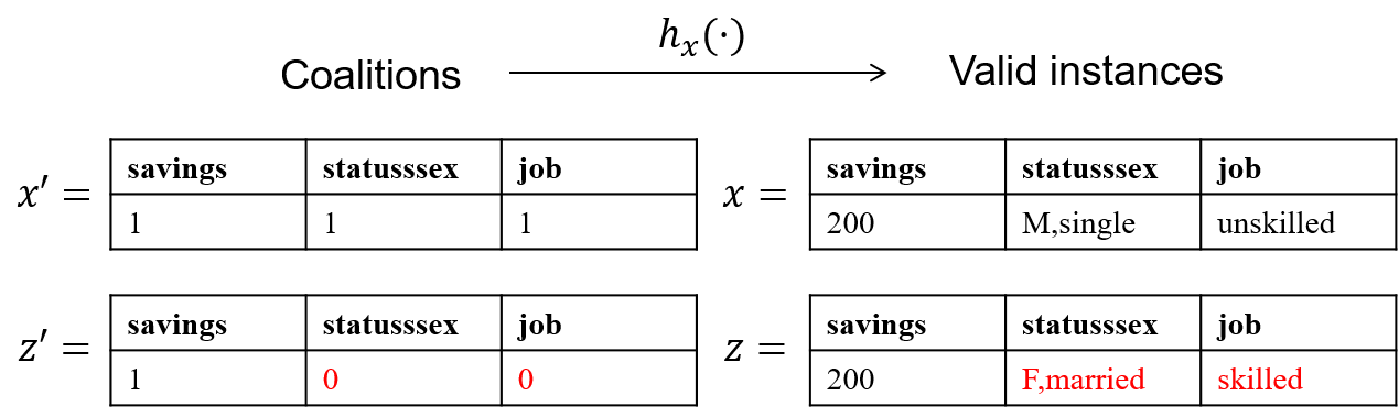
Figure 1: An example of a mapping function $h_{x}$ that converts coalitions to valid instances (i.e., instances in the feature space).

Both LIME and SHAP only provide explanations for individual (local) predictions. However, in order to detect unintended bias, a global understanding of the inner workings of the ML model is needed. In the following subsection we recall a simple strategy to obtain global explanations from individual explanations.

II-B3 From Local to Global Explanations

Local explanation methods have been used to explain individual predictions. However, they only provide local explanations which alone cannot provide a global understanding of ML models. To overcome this issue, Ribeiro et al. [11] proposed the so-called Submodular-pick (SP) for selecting a subset of local explanations that helps in interpreting the global behavior of any ML model. SP was originally proposed to work along with LIME explanations and it is called SP-LIME. The main idea on which relies SP-LIME is to sample a set of instances whose explanations are not redundant and that has a “high covering” in the following sense.

Denote by $B$ the desired number of explanations used to explain $f$ globally, and let $V$ be a set of selected instances, $I$ an array of feature importance, and $W$ an explanation matrix –columns represent features and rows represent instances– that contains the importance (contribution) of $d^{\prime}$ features to each instance. SP-LIME picks instances that are explaining thanks to:

$$Pick(W,I)=\arg\max_{V,|V|<B}\sum_{j=1}^{d^{\prime}}\mathrm{1}_{[i\in V:\mathcal{W}_{ij}>0]}I_{j}.$$

III FixOut

In this section, we revisit the human-centered framework FixOut that tackles process fairness [10]. FixOut is model-agnostic and explainer-agnostic such that it can be applied on top of any ML model, and in addition it is also able to use any explanation method based on feature importance.

FixOut takes as input a quadruple $(M,D,S,E)$ of a pre-trained model $M$, a dataset $D$ used to train $M$, a set of sensitive features $S$, and an explanation method $E$. It is based on two main components which are made precise below.

The first component is in charge of assessing fairness of $M$. More precisely, explainer $E$ builds the list $L$ of features that contribute the most to the classifications of $M$ (function GlobalExplanations in the Algorithm 1). Here, users must indicate a value for the parameter $k$ that limits the size of this list. FixOut then applies the following rule: if at least one sensitive feature returned by $E$ appears in $L$, $M$ is deemed unfair. Otherwise, $M$ is deemed fair and no action is taken.

The second component is applied only if $M$ is deemed unfair. The goal of this component is to use feature dropout together with an ensemble approach to build an ensemble classifier $M_{final}$ which is less dependent on sensitive features –or fairer– than $M$ (see Algorithm 1).

Let $S^{\prime}\subseteq S$ be the subset of sensitive features appearing in $L$. FixOut uses feature dropout to train $|S^{\prime}|+1$ classifiers in the following way: $|S^{\prime}|$ classifiers are defined by removing each of the sensitive features in $S^{\prime}$, and an additional classifier is defined by removing all sensitive features in $S^{\prime}$.

Now, let $x$ be an instance, $C$ a class value, and $M_{t}$ the $t$-th classifier in the pool of classifiers. FixOut uses models that make classifications in the form of probabilities $P(x\in C)$. Once all classifiers are trained, they are then combined thanks to an aggregation function. LimeOut uses only a simple average while FixOut is able to employ either a simple or weighted average function.

The aggregation function is responsible for producing the final classification. The final probability of $x$ to belong to the class $C$ is based on the probabilities $P(x\in C)$ obtained from the pool of classifiers and it is defined as the simple average:

$$P_{M_{final}}(x\in C)=\frac{1}{|S^{\prime}|+1}\sum_{t=1}^{|S^{\prime}|+1}P_{M_{t}}(x\in C),$$ (3)

where $P_{M_{t}}(x\in C)$ is the probability predicted by model $M_{t}$.

Data: $M$: pre-trained model; $D$: dataset; $S$: sensitive features; $E$: explainer; $k$: number of features considered.

Result: $M_{final}$ an ensemble model.

1

2$L\leftarrow\textsc{GlobalExplanations}(E,M,D,k)$

3 $S^{\prime}\leftarrow\{s_{t}\mid s_{t}\in S\wedge s_{t}\in L\}$

4 if $|S^{\prime}|>0$ then

5       $M_{final}\leftarrow\{\textsc{Train}(M_{t},D-\{s_{t}\})\mid s_{t}\in S^{\prime}\}$

6       $M_{final}\leftarrow M_{final}\cup\textsc{Train}(M_{t+1},D-S^{\prime})$

7       return $M_{final}$

8      

9

Algorithm 1 FixOut

TABLE I: An example of global explanations for Random Forest on the German dataset.

Original (SHAP)
Feature	Contrib.
statussex	-10.758909
property	10.676458
credithistory	10.264842
residencesince	8.108638
employmentsince	6.818476
existingchecking	6.308758
housing	-5.649528
installmentrate	5.125154
duration	4.838629
telephone	3.981387

FixOut using SHAP
Feature	Contrib.
credithistory	13.246923
employmentsince	9.550589
property	8.958718
residencesince	7.264848
installmentrate	5.893469
housing	-3.829469
statussex	-3.313667
duration	2.678797
existingcredits	2.412488
telephone	2.269493

IV Automating the choice of $k$

In order to assess fairness of ML models, FixOut only takes into account the first $k$ most important features. Thus, FixOut practitioners must know beforehand a suitable value for $k$ so that FixOut builds $L$ with the $k$ most important features. The system then looks at whether sensitive features are in $L$. An inappropriate value for $k$ prevents FixOut of correctly detecting unfairness issues as all sensitive features may not appear in $L$.

In this section, we propose an algorithm that automates the choice of $k$, based on the statistical measure kurtosis. Indeed kurtosis indicates the flatness of a distribution. Let $X=(x_{i})_{i\in\mathbb{N}}$ be a random variable, the kurtosis $\gamma$ of $X$ is defined as follows:

$$\gamma(X)=\frac{1}{n}\sum_{x_{i}}\left(\frac{x_{i}-\mu}{\sigma}\right)^{4},$$

where $\sigma$ is the standard deviation, $\mu$ is the mean, $x_{i}$ is a sample of $X$. For instance, $\gamma(X)<3$ indicates that $X$ is platykurtic (flattened), while $\gamma(X)=3$ defines a mesokurtic distribution (which is the case of normal distribution), and $\gamma(X)>3$ indicates that the distribution is leptokurtic (pointed) [21, 22].

Accordingly we propose the iterative algorithm called Find-K (see Algorithm 2), that selects a sub-sample of features of $L$ based on the kurtosis measure. Find-K removes features from $L$ by analyzing the kurtosis $\gamma(L)$ of $L$ before and after the deletion of a subset of features. For that, it iteratively removes features from the less important to the most important. The idea on which relies this algorithm is that once a feature is removed, the kurtosis of $L$ changes. The algorithm stops when $|\gamma(L)-\gamma(L^{\prime})|>\alpha$, where $L$ is the original list, $L^{\prime}$ is the list obtained after removing features, and $\alpha>0$ is a parameter.

Data: $L$: sorted list of contributions of all features (descending order); $\alpha$: a threshold.

Result: $L^{\prime}$ a new list of contributions of subset of features.

1

2$L^{\prime}\leftarrow L$

3 for $i\leftarrow|L|$ to $2$ do

4       $L^{\prime}\leftarrow L^{\prime}-L^{\prime}[i]$

5       if $|\gamma(L)-\gamma(L^{\prime})|>\alpha$ then

6             break

7      

8 end for

Algorithm 2 Find-K

V FixOut on Textual Data

In this section we demonstrate the adaptability of the FixOut framework to another data type, namely textual data. In this setting, a data instance corresponds to a text and features to words, i.e., the number of features is equal to the vocabulary size. To drop a feature, we remove each occurrence of the corresponding word in the text. Here words that are semantically equivalent are not taken into account.

Let $M$ be a classifier for which we want to reduce the impact of words from a given set $S$, in the classifier’s outcomes:

$$S=\{s_{i}\mid 1\leqslant i\leqslant n\}.$$

As in tabular data, FixOut decreases the contribution of the words in $S$ to the classifiers outcomes by applying feature dropout and by building an ensemble of the $n+1$ classifiers:

• one classifier $M_{i}$, for $1\leqslant i\leqslant n$, trained by ignoring the word $s_{i}$, and

• a classifier $M_{[n+1]}$ trained by ignoring all words in $S$.

However, when $n$ is large, this method becomes inefficient, for two reasons. The first one is that if we consider a sensitive word $s_{i}\in S$, only two classifiers are ignoring it: $M_{i}$ and $M_{[n+1]}$, i.e., $n-1$ out of the $n+1$ classifiers are taking the feature $s_{i}$ into account. Hence, the dropout of $s_{i}$ may then become less significant when $n$ is large. The second reason is a complexity concern: the more models there are, the more memory and computation time the ensemble takes.

Table II shows satisfactory results for a random forest model, which classifies a text as hate speech or not (from the hatespeech database, which is described later). We select $n=$ 3 words for which we want to reduce the contribution. The list of words used here was inspired by the analysis performed in [5]. We train a new model and globally explain it 50 times (with Random Sampling), in order to retrieve an average contribution. We can check that the rank of importance and contribution of each dropped feature decreases thanks to the FixOut ensemble. We evaluate the gain by calculating the difference between the rank obtained and the starting rank, normalised by the smaller of the two. Gaining a few ranks on the highest features in the ranking allows us to have significant scores, whereas they will be close to 0 for ranks that are very far away. However, when $n$ increases and more than 3 words are added, the method seems to become less effective, as shown in Table III (without grouping), which describes the rank and contribution of each one of the selected words whose importance should be reduced.

Let us turn our attention to the interest of grouping words. Instead of ignoring a single word or feature, the classifier can drop many words at the same time, then reducing the size of the ensemble. We proceeded in this way and the performance of FixOut was improved as it can be observed in Table III.

TABLE II: Process fairness assessment on a hate speech classifier (random forest), global explanation with SHAP RS, selecting 3 words

	Original model		FixOut Ensemble		Diff
Word	Rank	Contrib.	Rank	Contrib.	Rank
niggah	14	0.176	30	0.043	1.14
nigger	12	0.213	29	0.045	1.41
nig	7	0.276	55	0.021	6.85

TABLE III: Process fairness assessment on a hate speech classifier (random forest), global explanation with SHAP RS, selecting 7 words

	Without grouping		With grouping		Diff
Word	Rank	Contrib.	Rank	Contrib.	Rank
niggah	18	0.149	23	0.03	0.27
nigger	15	0.164	21	0.031	0.40
nigguh	22	0.13	83	0.008	2.77
nig	12	0.202	65	0.011	4.41
nicca	22	0.107	39	0.018	0.77
nigga	20	0.125	12	0.067	-0.66
white	25	0.087	36	0.018	0.44

VI Experimental Results and Discussion

The main goal of the experiments is to demonstrate the adaptability of FixOut on different data types. This section is thus divided in two main parts, the first one focusing on tabular data and the second one on textual data. We start by describing the tabular datasets (§ V). We then discuss the empirical results related to the selection of instances for assessing fairness (§ VI-B), and the automation of the choice of $k$ (§ VI-C). We end up this section by describing the textual dataset (§ VI-D) and by discussing the results obtained from the experiments performed on this data type (§ VI-E).

VI-A Tabular Datasets

The experiments on tabular data were performed on 3 real-world datasets, which contain sensitive features and are briefly outlined below.

German. This dataset contains 1000 instances and it is available in the UCI repository. For this dataset, the goal is to predict if the credit risk of a person is good or bad. Each applicant is described by 20 features in total out of which 3 features, namely “statussex”, “telephone”, “foreign worker”, are considered as sensitive.

Adult. This dataset is also available in the UCI repository. The task is to predict whether the salary of a American citizen exceeds 50 thousand dollars per year based on census data. It contains more than 32000 instances. Each data instance is described by 14 features out of which 3 features are considered as sensitive, namely “MaritalStatus”, “Race”, “Sex”.

LSAC. This dataset contains information about 26551 law students. The task is to classify whether law students pass the bar exam based on information from the study of the Law School Admission Council that was collected between 1991 and 1997. Each student is characterized by 11 features out of which 3 features, namely “race”, “sex”, “family_income”, are considered as sensitive.

We split each dataset into 70% for the training set and 30% for testing. We then applied the Synthetic Minority Oversampling Technique (SMOTE) over training data as class labels are highly imbalanced. In particular, SMOTE generates samples to balance the class label distribution in order to overcome the imbalanced distribution problem.

VI-B Tabular data: Selection of instances to assess fairness

We experimented different relative sizes for sampling instances. The idea is to verify whether at least one sensitive feature appears in the list of the top-10 most important features. For that, we used the following the relative sizes: 0.1%, 0.5%, 1%, 5%, and 10%. The results obtained throughout the performance of the same experiment 50 times are shown in Table IV.

For the German dataset, we did not evaluate models using 0.1% of the instances, as it takes only one instance. On the other hand, for the Adult dataset, the amount of data instances from sampling 10% of instances is large and unfeasible to produce many explanations (more than 3K) in time. We thus add an hyphen in Table IV to indicate these particular cases.

TABLE IV: Number of times pre-trained models are deemed unfair. Experiments were performed by varying the number of instances selected to obtain global explanations, the sampling strategy, and the explanation method.

Dataset	Selection	Sample size
		0.1%	0.5%	1%	5%	10%
German	LIME+RS	-	38	38	47	50
	LIME+SP	-	47	47	50	50
	SHAP+RS	-	50	50	50	50
	SHAP+SP	-	50	50	50	50
Adult	LIME+RS	46	48	49	45	-
	LIME+SP	49	49	49	49	-
	SHAP+RS	49	47	46	47	-
	SHAP+SP	47	50	49	49	-
LSAC	LIME+RS	50	50	50	50	50
	LIME+SP	50	50	50	50	50
	SHAP+RS	50	50	50	50	50
	SHAP+SP	50	50	50	50	50

To illustrate the impact of the sample size and the sampling method in the assessment of fairness, we observed the rank of sensitive features in the list of 10 most important features obtained by each of the explainers. These results are presented in Tables V, VI, and VII for the datasets German, Adult, and LSAC, respectively.

TABLE V: Rank of sensitive features in $L$ (and their average contribution): Effects of the variation of the sample size on the German dataset.

	Sensitive	Selection	Sample size
	feature		0.1%		0.5%		1%		5%		10%
German	sex	LIME+RS	-	(-)	5	(-0.015)	4	(-0.117)	2	(-1.630)	9	(-2.568)
		LIME+SP	-	(-)	6	(-0.147)	3	(-0.397)	6	(-1.610)	4	(-3.063)
		SHAP+RS	-	(-)	1	(-0.345)	1	(-0.345)	0	(-3.135)	0	(-6.836)
		SHAP+SP	-	(-)	0	(0.360)	0	(0.617)	0	(3.123)	0	(6.853)
	telephone	LIME+RS	-	(-)	3	(0.003)	8	(0.095)	6	(1.509)	9	(2.891)
		LIME+SP	-	(-)	3	(0.023)	5	(0.256)	6	(1.431)	7	(2.261)
		SHAP+RS	-	(-)	7	(0.121)	7	(0.121)	5	(1.245)	5	(2.753)
		SHAP+SP	-	(-)	2	(-0.156)	4	(-0.328)	5	(-1.180)	4	(-2.428)
	foreign	LIME+RS	-	(-)	2	(0.041)	9	(0.076)	8	(1.078)	6	(3.294)
		LIME+SP	-	(-)	1	(0.376)	0	(0.721)	0	(3.289)	0	(7.103)
		SHAP+RS	-	(-)	9	(0.122)	9	(0.122)	9	(0.490)	*	*
		SHAP+SP	-	(-)	7	(-0.100)	9	(-0.114)	9	(-0.444)	9	(-1.011)

TABLE VI: Rank of sensitive features in $L$ (and their average contribution): Effects of the variation of the sample size on the Adult dataset.

	Sensitive	Selection	Sample size
	feature		0.1%		0.5%		1%		5%		10%
Adult	marital	LIME+RS	9	(-0.122)	9	(-0.012)	8	(0.138)	9	(2.146)	-	(-)
		LIME+SP	6	(0.042)	9	(0.367)	8	(0.244)	8	(2.746)	-	(-)
		SHAP+RS	7	(-0.003)	9	(-0.239)	8	(-0.246)	7	(-0.678)	-	(-)
		SHAP+SP	8	(0.030)	9	(0.093)	7	(0.296)	9	(1.731)	-	(-)
	race	LIME+RS	9	(0.012)	6	(-0.088)	6	(-0.253)	7	(-0.093)	-	(-)
		LIME+SP	9	(-0.009)	8	(-0.018)	7	(0.002)	7	(-0.002)	-	(-)
		SHAP+RS	9	(0.000)	6	(0.000)	8	(0.000)	6	(0.000)	-	(-)
		SHAP+SP	5	(0.000)	7	(0.000)	7	(0.001)	7	(0.000)	-	(-)
	sex	LIME+RS	4	(-0.022)	7	(0.305)	8	(0.617)	8	(4.902)	-	(-)
		LIME+SP	6	(0.153)	7	(0.823)	7	(0.484)	6	(6.925)	-	(-)
		SHAP+RS	7	(0.050)	6	(0.513)	6	(1.138)	6	(2.787)	-	(-)
		SHAP+SP	7	(-0.113)	6	(-0.203)	6	(-0.819)	6	(-3.387)	-	(-)

TABLE VII: Rank of sensitive features in $L$ (and their average contribution): Effects of the variation of the sample size on the LSAC dataset.

	Sensitive	Selection	Sample size
	feature		0.1%		0.5%		1%		5%		10%
LSAC		LIME+RS	9	(0.045)	9	(-0.962)	9	(-1.808)	9	(-6.754)	9	(-15.629)
		LIME+SP	9	(-0.143)	9	(-0.948)	9	(-2.004)	9	(-7.074)	9	(-15.194)
		SHAP+RS	3	(-0.445)	2	(-1.986)	1	(-4.071)	1	(-18.311)	1	(-31.343)
	sex	SHAP+SP	2	(0.477)	1	(1.827)	1	(4.943)	1	(14.738)	1	(46.189)
		LIME+RS	6	(0.735)	3	(6.309)	3	(13.561)	6	(67.047)	6	(129.130)
		LIME+SP	5	(1.222)	3	(6.827)	6	(12.202)	3	(65.198)	6	(132.644)
		SHAP+RS	4	(0.346)	3	(1.633)	2	(2.886)	3	(14.858)	3	(29.474)
	race	SHAP+SP	7	(-0.275)	2	(-1.385)	3	(-2.724)	3	(-15.227)	3	(-27.966)
		LIME+RS	8	(-0.289)	9	(-1.901)	9	(-2.342)	9	(-16.258)	7	(-45.129)
		LIME+SP	9	(-0.454)	9	(-2.250)	7	(-4.351)	7	(-25.473)	7	(-44.837)
		SHAP+RS	8	(0.119)	8	(0.487)	9	(0.812)	4	(3.913)	3	(11.642)
	f_income	SHAP+SP	8	(-0.029)	6	(-0.568)	7	(-0.989)	6	(-4.576)	6	(-6.047)

We considered the following classifiers, namely Logistic Regression (LR), Bagging (BAG), AdaBoost (ADA), and Random Forest (RF), to perform the experiments. We used the implementation available on Scikit-learn [23] with the default parameters. Based on these results we thus set the size as 5% for the German dataset (50 instances), 0.5% for the Adult dataset (162 instances), and 0.1% for the LSAC dataset (93 instances). These results seem to indicate that LIME is more stable than SHAP independently of the sampling method and sample size.

VI-C Tabular data: Automating the choice of $k$

We evaluate the algorithm Find-K that was conceived to automatically selects the list of features which is taken into account by FixOut for assessing fairness. Find-K requires a positive value for the parameter $\alpha$. Here, we performed experiments by varying the value of $\alpha$ from 0.5 to 3. In these experiments we analyze the impact of this parameter on the output of Find-K. In particular, we are interested in the effects of different values of $\alpha$ w.r.t. the size of $L$ (i.e., the number of features kept by Find-K) and record the number of times a model is deemed unfair. We discarded values of $\alpha<0.5$ otherwise Find-K considers all features as important.

TABLE VIII: Average value of $k$ for LR and BAG classifiers (number of times models are deemed unfair): Effects of the variation of $\alpha$ over the number of features kept by Find-K.

Data.	Selection	LR												BAG
		$\alpha$												$\alpha$
		0.5		1		1.5		2		2.5		3		0.5		1		1.5		2		2.5		3
German	LIME+RS	9.9	(47)	8.7	(42)	6.8	(31)	5.5	(23)	3.5	(13)	2.6	(8)	10.0	(33)	9.58	(31)	8.18	(24)	6.38	(18)	4.26	(8)	2.82	(2)
	LIME+SP	9.7	(50)	8.2	(49)	6.1	(43)	4.5	(39)	2.1	(29)	1.3	(24)	10.0	(41)	10.0	(41)	9.74	(41)	9.08	(40)	7.04	(30)	4.86	(21)
	SHAP+RS	10.0	(50)	9.9	(50)	9.5	(50)	7.4	(47)	5.7	(45)	3.8	(43)	9.92	(37)	9.80	(37)	8.78	(33)	7.16	(26)	5.86	(22)	4.86	(19)
	SHAP+SP	10.0	(50)	9.8	(50)	8.9	(50)	7.0	(49)	5.4	(45)	4.0	(43)	10.0	(45)	9.78	(45)	9.12	(43)	7.72	(36)	6.58	(31)	5.50	(26)
Adult	LIME+RS	10.0	(46)	10.0	(46)	10.0	(46)	9.9	(46)	9.9	(44)	9.8	(44)	10.0	(49)	10.0	(49)	10.0	(49)	9.58	(49)	8.32	(45)	6.82	(40)
	LIME+SP	10.0	(49)	10.0	(49)	10.0	(49)	10.0	(49)	9.9	(49)	9.8	(49)	10.0	(50)	10.0	(50)	10.0	(50)	9.64	(50)	8.52	(50)	7.32	(50)
	SHAP+RS	10.0	(48)	10.0	(48)	10.0	(48)	10.0	(48)	9.8	(48)	9.7	(45)	10.0	(49)	10.0	(49)	10.0	(49)	9.62	(49)	8.30	(45)	7.08	(40)
	SHAP+SP	10.0	(50)	9.9	(50)	9.8	(50)	9.7	(50)	9.6	(49)	9.3	(49)	10.0	(50)	10.0	(50)	8.84	(50)	5.84	(39)	2.32	(11)	1.32	(2)
LSAC	LIME+RS	8.6	(47)	6.4	(28)	4.0	(10)	2.5	(6)	1.8	(1)	1.3	(0)	7.74	(50)	5.64	(49)	4.04	(43)	2.68	(32)	1.98	(24)	1.56	(21)
	LIME+SP	7.7	(35)	5.1	(22)	3.1	(14)	1.7	(4)	1.1	(0)	1.0	(0)	9.72	(50)	8.76	(50)	7.86	(50)	7.00	(50)	5.96	(49)	4.84	(44)
	SHAP+RS	8.5	(48)	6.6	(42)	4.5	(30)	3.2	(22)	2.5	(18)	2.0	(12)	8.34	(50)	5.98	(32)	4.46	(24)	3.04	(17)	2.56	(14)	2.08	(11)
	SHAP+SP	8.3	(50)	6.1	(45)	4.4	(36)	3.2	(26)	2.3	(19)	1.7	(14)	8.70	(49)	6.88	(44)	5.10	(33)	3.76	(26)	2.82	(14)	2.22	(11)

TABLE IX: Average value of $k$ for RF and ADA classifiers (number of times models are deemed unfair): Effects of the variation of $\alpha$ over the number of features kept by Find-K.

Data.	Selection	RF												ADA
		$\alpha$												$\alpha$
		0.5		1		1.5		2		2.5		3		0.5		1		1.5		2		2.5		3
German	LIME+RS	9.90	(49)	8.30	(43)	5.18	(25)	2.72	(8)	1.54	(2)	1.18	(2)	10	(48)	10	(48)	9.76	(48)	9.4	(46)	9.2	(45)	9.04	(44)
	LIME+SP	10.0	(50)	9.98	(50)	9.74	(50)	8.54	(50)	6.96	(47)	5.46	(46)	10.0	(50)	10.0	(50)	10.0	(50)	10.0	(50)	10.0	(50)	10.0	(50)
	SHAP+RS	9.92	(50)	8.98	(48)	6.46	(39)	4.52	(29)	2.74	(23)	2.04	(18)	10.0	(48)	8.78	(43)	6.44	(31)	4.28	(23)	3.24	(15)	2.90	(13)
	SHAP+SP	9.86	(50)	8.70	(47)	5.64	(33)	3.68	(27)	2.28	(22)	1.42	(17)	9.98	(47)	8.68	(42)	6.78	(34)	5.82	(30)	4.92	(24)	4.04	(20)
Adult	LIME+RS	9.76	(50)	8.38	(50)	7.00	(48)	5.48	(38)	4.44	(18)	3.64	(6)	10.0	(50)	10.0	(50)	8.22	(49)	5.54	(35)	3.40	(13)	2.20	(2)
	LIME+SP	9.30	(50)	7.80	(50)	6.76	(50)	5.80	(48)	5.00	(40)	4.32	(27)	10.0	(50)	9.90	(50)	7.98	(49)	5.74	(43)	3.84	(19)	2.48	(4)
	SHAP+RS	10.0	(50)	9.96	(50)	9.30	(50)	8.12	(50)	6.48	(46)	5.14	(41)	10.0	(50)	9.02	(50)	6.62	(49)	4.76	(48)	3.28	(47)	2.38	(47)
	SHAP+SP	10.0	(50)	9.98	(50)	9.38	(50)	8.02	(48)	6.26	(47)	4.94	(38)	10.0	(50)	9.16	(49)	7.22	(49)	5.36	(49)	4.06	(47)	2.82	(47)
LSAC	LIME+RS	6.46	(49)	4.04	(38)	2.02	(16)	1.46	(10)	1.10	(6)	1.02	(6)	6.98	(44)	4.52	(32)	3.02	(20)	1.92	(11)	1.28	(5)	1.12	(4)
	LIME+SP	8.92	(50)	7.30	(49)	5.38	(48)	3.66	(48)	2.66	(48)	1.96	(48)	7.08	(46)	5.06	(34)	3.44	(22)	2.22	(11)	1.78	(9)	1.28	(4)
	SHAP+RS	7.80	(47)	5.80	(40)	3.88	(21)	2.48	(13)	1.76	(7)	1.40	(3)	8.68	(50)	6.52	(42)	4.78	(30)	3.34	(21)	2.08	(8)	1.52	(6)
	SHAP+SP	8.18	(49)	5.78	(37)	4.04	(23)	2.86	(13)	2.10	(8)	1.70	(4)	8.84	(50)	7.08	(47)	5.42	(39)	3.84	(26)	2.68	(12)	1.90	(7)

High values of $\alpha$ lead to a smaller size of $L$, i.e., too many features are removed by Find-K. It is harder to find one sensitive feature in a very short list of important features than in a longer list. As a consequence, high values of $\alpha$ also lead to a low number of times in which a model is deemed unfair. We can observe this behavior on Tables VIII and IX. These tables contain the number of times that the models were deemed unfair throughout 50 repetitions of the same experiment.

A similar behavior can be observed w.r.t. the average value of $k$. High values of $\alpha$ lead to low values of $k$ (on average). We notice this behavior in Tables VIII and IX. These tables contain the average value of $k$ found by Find-K. We highlighted the experiments where the average number of sensitive features found in the list obtained by FixOut was greater than or equal to 1. Again, FixOut looks for at least one sensitive feature in the list of the most important features. Then, an average smaller than 1 indicates that in most experiments the models were deemed fair. We also notice that the highlighted values are those in which the average value of $k$ are high (see Tables VIII and IX).

We can observe that Find-K discovers on average the same value of $k$ for each dataset. For instance, for the German dataset, an average $k$ around 10 was found by Find-K with $\alpha=0.5$, and incidentally the same value was used in previous empirical studies [9, 10]. For the LSAC dataset, an average $k$ around 8 was found using Find-K with $\alpha=0.5$, while an average $k$ around 6 was returned by Find-K using $\alpha=1$.

To sum up the analysis of Find-K, we can also observe that low values of $\alpha$ provide suitable configurations for users that do not have any clue of the useful values of $k$. More precisely, using $0.5\leq\alpha\leq 1$ allows Find-K to automatically find a suitable value of $k$. In addition, since LIME and SHAP have stability issues [24] that lead to different lists of feature importance (for a single type of classifier trained on the same dataset), it may be interesting to considering the threshold $\alpha$ to learn the parameter $k$. Indeed, one single value of $\alpha$ allows Find-K to find a suitable value of $k$ from distinct lists of feature importance. This provides an answer to question Q1 introduced at the beginning of this paper.

VI-D Textual datasets

We also experimented FixOut with simple textual classifiers. In particular, we implemented a model used in an experiment carried out by Davidson et al. [5], whose goal is to classify tweets as hate speech or not. We focus on the hate speech dataset [25], which more precisely labels a tweet as offensive, hate speech, or neither. To stay within a two-classes problem, we merge offensive language and hate speech classes, to finally deal with two classes, namely non-offensive or offensive.

However, the resulting dataset appears to be quite unbalanced, including 4163 non-offensive instances and 20620 offensive ones. Thus we randomly select only 4163 instances from the offensive group. Moreover, we follow the same representation and pre-processing steps as in [5]. We stem each word in order to reduce and to gather similar words, e.g., “vehicle” and “vehicles” are both transformed into “vehicl”. The classifier is based on a TF-IDF vectorizer followed by a logistic regression. In addition, we ran experiments with a bagging ensemble, a random forest, and AdaBoost, instead of the logistic regression.

Then we apply the first step of FixOut to build a global explanation. This is performed with the textual adaptation of LIME and SHAP. We compare both random sampling (RS) and submodular pick (SP), for these two explainers. Unlike the previous tabular classifiers, the model deals with more than 2000 features, i.e., as many as the vocabulary size. For example, Table X shows the first 10 most important words obtained after 50 experiments run with a logistic regression and LIME explanations, respectively with random sampling and submodular pick.

TABLE X: Mean contribution of a logistic regression, LIME as explainer, after 50 experiments

Random sampling
rank	word	contrib.
1	faggot	0.632
2	fag	0.625
3	bitch	0.622
4	niggah	0.620
5	cunt	0.613
6	pussi	0.608
7	nigger	0.597
8	hoe	0.580
9	nigguh	0.522
10	dyke	0.473

Submodular pick
rank	word	contrib.
1	niggah	0.596
2	cunt	0.579
3	bitch	0.574
4	fag	0.573
5	faggot	0.573
6	nigger	0.572
7	pussi	0.547
8	hoe	0.524
9	nigguh	0.505
10	retard	0.414

At first glance, we can observe that important words for hate speech classification are insults and swear words, which makes sense. However, it should be noticed that such a classification may also be related to a particular context. For example, the use of words such as “n*gger” in a conversation may also be related to a familiar interaction between two very close friends, and thus not at all indicate an offensive discussion.

This shows that the definition of a sensitive word is not straightforward in such a case, and that we must find words that are responsible for a bias. Then, in order to complete this experiment, we manually select sensitive features. Accordingly, the objective of the next subsection is to demonstrate that FixOut is able to decrease the contribution of pre-selected words thanks to a FixOut ensemble and by grouping words. For example, considering the groups of words presented in Figure 2, the goal of this ensemble is to reduce the contribution of these groups of words.

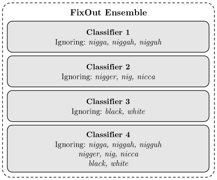
Figure 2: Illustration of textual classifiers used in the ensemble.

VI-E Textual data: Process fairness assessment

For each experiment, we train 4 models, namely logistic regression, random forest, adaboost, and bagging, plus 4 models corresponding to the related FixOut ensembles, which should be less dependent to sensitive words as defined above. Next, we use LIME and SHAP explanations, with both random sampling and submodular pick. For each explanation, we assess the contribution of all the features. We then sort all the features w.r.t. their average contribution, select the 500 most important words, and then check their rank. Words which are not in this list are therefore ranked beyond 500 and their contribution is marked as “ - ” to indicate that it is not significant.

Table XI shows the results obtained with random sampling, including ranking difference. LIME explanations systematically show a decrease in the contribution and the importance rank of selected words. We even observe that the contribution is often nearly divided by 2, although the contribution of the whole vocabulary tends to decrease a bit in the ensemble explanation. By contrast, SHAP explanations show an increase in the ranking of the word nigga, although its contribution decreases. The contribution of all other selected words is decreasing in general, even if this tendency seems to be more instable than in the case of LIME. Table XI also presents the results obtained with submodular pick, and shows results similar to random sampling with better results with logistic regression (+1.22 in average with LIME and +1.90 with SHAP). These latter results seem to indicate that FixOut with LIME explanations is more stable and consistently improves process fairness, i.e., always decrease the contribution of sensitive features. However, FixOut with SHAP seems to provide greater improvements; see, e.g., “nigguh” and “nig” in the case of LR (diff. rank 22.81 and 54.56 with submodular pick and 21.73 and 40.67 with random sampling, resp.). It is noteworthy that for SHAP “nigga” always worsens.

TABLE XI: Process fairness assessment on textual data, global explanations with submodular pick and random sampling, respectively.

		Original model		FixOut Ensemble		Diff
	Word	Rank	Contrib.	Rank	Contrib.	Rank
LR, LIME+SP	niggah	1	0.596	12	0.275	11
	nigger	6	0.572	13	0.274	1.16
	nigguh	9	0.505	14	0.269	0.55
	nig	13	0.315	20	0.138	0.54
	nicca	15	0.289	23	0.12	0.53
	nigga	18	0.24	24	0.119	0.33
	white	23	0.178	45	0.096	0.96
	black	145	0.047	323	0.028	1.23
RF, LIME+SP	niggah	7	0.517	12	0.257	0.71
	nigger	9	0.476	15	0.23	0.67
	nigguh	13	0.339	17	0.194	0.31
	nig	10	0.445	16	0.204	0.60
	nicca	16	0.265	20	0.121	0.25
	nigga	17	0.235	23	0.112	0.35
	white	23	0.127	34	0.07	0.48
	black	$>$500	$\sim 0$	$>$500	$\sim 0$	0.00
ADA, LIME+SP	niggah	2	0.167	4	0.083	1.00
	nigger	7	0.052	10	0.026	0.43
	nigguh	5	0.144	6	0.073	0.20
	nig	18	0.014	24	0.006	0.33
	nicca	17	0.015	23	0.007	0.35
	nigga	4	0.166	5	0.083	0.25
	white	23	0.011	26	0.005	0.13
	black	113	0.0	196	0.0	0.73
BAG, LIME+SP	niggah	5	0.645	15	0.293	2.00
	nigger	11	0.58	16	0.29	0.45
	nigguh	13	0.497	18	0.233	0.38
	nig	1	0.659	10	0.336	9.00
	nicca	15	0.387	19	0.195	0.27
	nigga	19	0.285	21	0.139	0.11
	white	21	0.183	24	0.083	0.14
	black	420	0.004	$>$500	$\sim 0$	0.19

		Original model		FixOut Ensemble		Diff
	Word	Rank	Contrib.	Rank	Contrib.	Rank
LR, SHAP+SP	niggah	16	0.179	75	0.015	3.69
	nigger	11	0.239	23	0.034	1.09
	nigguh	21	0.123	$>$500	$\sim 0$	22.81
	nig	9	0.249	$>$500	$\sim 0$	54.56
	nicca	22	0.12	46	0.02	1,09
	nigga	19	0.159	14	0.053	-0.36
	white	20	0.14	50	0.019	1,50
	black	$>$500	$\sim 0$	$>$500	$\sim 0$	0.00
RF, SHAP+SP	niggah	14	0.176	23	0.03	0.64
	nigger	12	0.213	21	0.031	0.75
	nigguh	22	0.13	83	0.008	2.77
	nig	7	0.276	65	0.011	8.29
	nicca	21	0.138	39	0.018	0.86
	nigga	18	0.155	12	0.067	-0.50
	white	26	0.085	36	0.018	0.38
	black	$>$500	$\sim 0$	$>$500	$\sim 0$	0.00
ADA, SHAP+SP	niggah	5	0.05	11	0.007	1.20
	nigger	9	0.018	13	0.005	0.44
	nigguh	6	0.039	25	0.002	3.17
	nig	18	0.009	86	0.001	3.78
	nicca	34	0.006	40	0.001	0.18
	nigga	4	0.07	3	0.031	-0.33
	white	32	0.007	30	0.002	-0.07
	black	$>$500	$\sim 0$	$>$500	$\sim 0$	0.00
BAG, SHAP+SP	niggah	15	0.202	24	0.021	0.60
	nigger	12	0.28	17	0.038	0.42
	nigguh	19	0.166	44	0.012	1.32
	nig	2	0.508	14	0.044	6.00
	nicca	14	0.209	21	0.025	0.50
	nigga	17	0.195	11	0.078	-0.55
	white	25	0.074	72	0.008	1.88
	black	$>$500	$\sim 0$	$>$500	$\sim 0$	0.00

		Original model		FixOut Ensemble		Diff
	Word	Rank	Contrib.	Rank	Contrib.	Rank
LR, LIME+RS	niggah	4	0.62	12	0.277	2.00
	nigger	7	0.597	10	0.29	0.43
	nigguh	9	0.522	14	0.264	0.56
	nig	13	0.328	20	0.15	0.54
	nicca	14	0.316	22	0.134	0.57
	nigga	18	0.237	27	0.113	0.50
	white	23	0.172	35	0.104	0.52
	black	131	0.05	316	0.028	1.41
RF, LIME+RS	niggah	7	0.593	10	0.289	0.43
	nigger	9	0.497	14	0.236	0.56
	nigguh	13	0.358	17	0.198	0.31
	nig	10	0.46	16	0.222	0.60
	nicca	14	0.286	20	0.132	0.43
	nigga	18	0.23	23	0.112	0.28
	white	23	0.119	33	0.066	0.43
	black	$>$500	$\sim 0$	$>$500	$\sim 0$	0.00
ADA, LIME+RS	niggah	3	0.166	5	0.082	0.67
	nigger	7	0.052	11	0.026	0.57
	nigguh	5	0.144	6	0.074	0.20
	nig	18	0.014	24	0.006	0.33
	nicca	17	0.015	23	0.007	0.35
	nigga	4	0.166	4	0.083	0.00
	white	22	0.011	26	0.005	0.18
	black	115	0.0	192	0.0	0.67
BAG, LIME+RS	niggah	6	0.687	13	0.32	1.17
	nigger	10	0.629	15	0.306	0.50
	nigguh	13	0.535	17	0.248	0.31
	nig	2	0.7	10	0.353	4.00
	nicca	15	0.395	19	0.2	0.27
	nigga	19	0.284	21	0.139	0.11
	white	22	0.158	25	0.074	0.14
	black	$>$500	$\sim 0$	$>$500	$\sim 0$	0,00

		Original model		FixOut Ensemble		Diff
	Word	Rank	Contrib.	Rank	Contrib.	Rank
LR, SHAP+RS	niggah	16	0.194	68	0.016	3.25
	nigger	7	0.273	18	0.042	1.57
	nigguh	22	0.126	$>$500	$\sim 0$	21.73
	nig	12	0.223	$>$500	$\sim 0$	40.67
	nicca	21	0.138	37	0.024	0.76
	nigga	19	0.179	13	0.061	-0.46
	white	20	0.177	53	0.019	1.65
	black	$>$500	$\sim 0$	$>$500	$\sim 0$	0.00
RF, SHAP+RS	niggah	14	0.188	22	0.03	0.57
	nigger	12	0.219	21	0.031	0.75
	nigguh	23	0.132	84	0.008	2.65
	nig	10	0.272	68	0.011	5.80
	nicca	21	0.154	36	0.021	0.71
	nigga	17	0.17	12	0.075	-0.42
	white	25	0.11	38	0.019	0.52
	black	$>$500	$\sim 0$	$>$500	$\sim 0$	0.00
ADA, SHAP+RS	niggah	5	0.048	11	0.007	1.20
	nigger	9	0.019	13	0.005	0.44
	nigguh	6	0.039	24	0.002	3.00
	nig	20	0.008	80	0.001	3.00
	nicca	26	0.006	37	0.001	0.42
	nigga	4	0.072	3	0.031	-0.33
	white	22	0.008	28	0.002	0.27
	black	$>$500	$\sim 0$	$>$500	$\sim 0$	0.00
BAG, SHAP+RS	niggah	17	0.203	26	0.02	0.53
	nigger	13	0.257	16	0.039	0.23
	nigguh	19	0.165	46	0.012	1.42
	nig	2	0.442	14	0.044	6.00
	nicca	14	0.217	21	0.026	0.50
	nigga	16	0.206	11	0.082	-0.45
	white	24	0.091	53	0.009	1.21
	black	$>$500	$\sim 0$	$>$500	$\sim 0$	0.00

VII Conclusion

In this paper, we revisited the framework FixOut that was proposed to render fairer classification models when applied to tabular data. We extended FixOut in several ways. We integrated an approach to automate the choice of the list of the most important features to be taken into account during the fairness analysis. We also evaluated different sampling strategies for selecting instances when assessing fairness.

We also explored the adaptability of FixOut’s framework to classification models on textual data. For that, we adapted the notion of feature dropout to bag of words, followed by the ensemble strategy. Our empirical results showed the feasibility of this idea when rendering models fairer. Furthermore, the comparison of FixOut’s workflow with LIME and SHAP explanations indicated that, even though SHAP provides drastic improvements in some cases, FixOut with LIME explanations is more stable, and consistently results in fairer models; this is not the case when using SHAP explanations. Submodular pick gives better average results than random sampling and the best gain is obtained for Logistic regression for both LIME and SHAP (and for both SP and RS).

This contribution opens several avenues for future work. For instance, in the case of textual data it remains to automate the choice of the words that FixOut should take into account in the dropout approach based on bags of words. Furthermore, we are currently experimenting with more complex data types, such as graphs and other structured data. However, to guarantee competitive results, model specific explanations, namely, for deep neural approaches, need to be considered. This constitutes a topic of ongoing research.

References

- [1] N. Grgic-Hlaca et al., “The case for process fairness in learning: Feature selection for fair decision making,” in NIPS Symposium on Machine Learning and the Law, 2016, p. 2.
- [2] L. Dixon et al., “Measuring and mitigating unintended bias in text classification,” in AAAI/ACM AIES, 2018, pp. 67–73.
- [3] M. Hardt et al., “Equality of opportunity in supervised learning,” in NIPS, 2016, pp. 3323–3331.
- [4] D. Hangartner et al., “Monitoring hiring discrimination through online recruitment platforms,” Nature, vol. 589, no. 7843, pp. 572–576, 2021.
- [5] T. Davidson et al., “Racial bias in hate speech and abusive language detection datasets,” in Proceedings of the Third Workshop on Abusive Language Online, 2019, pp. 25–35.
- [6] K. Makhlouf et al., “On the applicability of machine learning fairness notions,” ACM SIGKDD Explorations, vol. 23, no. 1, pp. 14–23, 2021.
- [7] M. J. Kusner et al., “Counterfactual fairness,” in NeurIPS, 2017, pp. 4066–4076.
- [8] M. B. Zafar et al., “Fairness constraints: Mechanisms for fair classification,” in Artificial Intelligence and Statistics, 2017, pp. 962–970.
- [9] V. Bhargava et al., “LimeOut: An Ensemble Approach To Improve Process Fairness,” in ECML PKDD Int. Workshop XKDD, 2020, pp. 475–491.
- [10] G. Alves et al., “FixOut: an ensemble approach to fairer models,” HAL preprint hal:03033181, 2020.
- [11] M. T. Ribeiro et al., ““Why Should I Trust You?”: Explaining the predictions of any classifier,” in ACM SIGKDD, 2016, pp. 1135–1144.
- [12] O. Papakyriakopoulos et al., “Bias in word embeddings,” in FAccT, 2020, pp. 446–457.
- [13] M. B. Zafar et al., “Fairness beyond disparate treatment & disparate impact: Learning classification without disparate mistreatment,” in WWW, 2017, p. 1171–1180.
- [14] T. Speicher et al., “A unified approach to quantifying algorithmic unfairness: Measuring individual & group unfairness via inequality indices,” in ACM SIGKDD, 2018, pp. 2239–2248.
- [15] S. Wachter et al., “Counterfactual explanations without opening the black box: Automated decisions and the gdpr,” Harvard Journal of Law & Technology, vol. 31, no. 2, 2018.
- [16] R. Guidotti et al., “A survey of methods for explaining black box models,” ACM CSUR, vol. 51, no. 5, pp. 1–42, 2018.
- [17] S. M. Lundberg and S. Lee, “A unified approach to interpreting model predictions,” in NIPS, 2017, pp. 4765–4774.
- [18] J. Adebayo et al., “Sanity checks for saliency maps,” in NeurIPS, 2018, pp. 9525–9536.
- [19] B. Kim et al., “Interpretability beyond feature attribution: Quantitative testing with concept activation vectors (TCAV),” in ICML, 2018, pp. 2668–2677.
- [20] D. Garreau and U. von Luxburg, “Explaining the explainer: A first theoretical analysis of lime,” in AISTATS, 2020, pp. 1287–1296.
- [21] J. J. A. Moors, “The meaning of kurtosis: Darlington reexamined,” The American Statistician, vol. 40, no. 4, pp. 283–284, 1986.
- [22] G. Saporta, Probabilités, analyse des données et statistique. Editions Technip, 2006.
- [23] F. Pedregosa et al., “Scikit-learn: Machine learning in Python,” vol. 12, pp. 2825–2830, 2011.
- [24] D. Slack et al., “Fooling lime and shap: Adversarial attacks on post hoc explanation methods,” in AAAI/ACM AIES, 2020, pp. 180–186.
- [25] T. Davidson et al., “Automated hate speech detection and the problem of offensive language,” in ICWSM, 2017, pp. 512–515.