Next-Gen Gas Network Simulation

Abstract

To overcome many-query optimization, control, or uncertainty quantification work loads in reliable gas and energy network operations, model order reduction is the mathematical technology of choice. To this end, we enhance the model, solver and reductor components of the morgen platform, introduced in Himpe et al [J. Math. Ind. 11:13, 2021], and conclude with a mathematically, numerically and computationally favorable model-solver-reductor ensemble.

1 Model Order Reduction for Gas and Energy Networks

Computer-based simulation of gas transport in pipeline networks has been an industrial as well as academic field of interest since the earliest scientific computing systems [5]. Especially, the transient simulation of gas flow and the dynamic gas network behavior are the pinnacle discipline in this regard. The MATLAB-based morgen – Model Order Reduction for Gas and Energy Networks – platformcontinues this research by providing a modular open-source software simulation stack for the comparison and benchmarking of models (discretizations), solvers (time steppers), and reductors (model reduction algorithms) [3]. Beyond, selecting apposite simulator components or ranking model reduction methods, an overall goal is the acceleration of forward simulations, so that many-query tasks relying thereon, such as optimization, control or uncertainty quantification, benefit in terms of performance. In this work, we summarize and enhance the foundational work of [3] with additional details, and accompany version 1.1 of morgen.

1.1 Modules Overview

The morgen platform is organized into modules: models, solvers, reductors, networks and tests. The networks module holds topology and scenario data, and the tests module defines the simulation and model reduction experiments, thus, we summarize the currently available core modules: models, solvers, and reductors. The models module assembles a semi-discrete input-output system from a network topology. Currently, two spatially discrete ODE models are included (Table 1).

Name	Identifier	port-Hamiltonian?	Reference
Midpoint discretization	ode_mid	No	[3, Sec. 2.4.1]
Endpoint discretization	ode_end	Yes	[3, Sec. 2.4.2]

Table 1: Available models in morgen in version 1.1.

The solvers module computes a time-discrete output trajectory from a model and a scenario. Six ODE solvers are provided in the current version (Table 2).

Name	Identifier	Comment	Reference
Adaptive 2nd Order Rosenbrock	generic	uses ode23s	[3, Sec. 5.3.1]
1st Order Implicit-Explicit	imex1	non-Runge-Kutta	[3, Sec. 5.3.3]
2nd Order Implicit-Explicit	imex2	Runge-Kutta	[3, Sec. 5.3.4]
Explicit 4th Order Runge-Kutta	rk4		[3, Sec. 5.3.2]
Explicit 2nd Order Runge-Kutta	rk2hyp	increased stability	[9]
Explicit 4th Order Runge-Kutta	rh4hyp	increased stability	[6]

Table 2: Available solvers in morgen in version 1.1.

The reductors module compresses a model given a solver and (generic training) scenario. All in all, $23$ reductors organized in four classes are available (Table 3).

Name	Identifier	Linear Variant	Reference
Proper Orthogonal Decomposition	pod_r	–	[3, Sec. 4.2]
Empirical Dominant Subspaces	eds_ro	eds_ro_l	[3, Sec. 4.3]
Empirical Dominant Subspaces	eds_wx	eds_wx_l	[3, Sec. 4.3]
Empirical Dominant Subspaces	eds_wz	eds_wz_l	[3, Sec. 4.3]
Balanced POD	bpod_ro	bpod_ro_l	[3, Sec. 4.4.3]
Balanced Truncation	ebt_ro	ebt_ro_l	[3, Sec. 4.4]
Balanced Truncation	ebt_wx	ebt_wx_l	[3, Sec. 4.4]
Balanced Truncation	ebt_wz	ebt_wz_l	[3, Sec. 4.4]
Goal-Oriented POD	gopod_r	–	[3, Sec. 4.5.1]
Balanced Gains	ebg_ro	ebg_ro_l	[3, Sec. 4.5]
Balanced Gains	ebg_wx	ebg_wx_l	[3, Sec. 4.5]
Balanced Gains	ebg_wz	ebg_wz_l	[3, Sec. 4.5]
DMD Galerkin	dmd_r	–	[3, Sec. 4.6]

Table 3: Available reductors in morgen in version 1.1.

2 Enhanced Functionality

In this section we discuss some properties of the morgen platform. Specifically, one aspect of each of the core modules (model, solver, reductor) is addressed. Additionally, further network/scenario data-sets were added in version 1.1, too.

2.1 Gravity Term

One component of the gas pipeline model, particularly of the retarding forces in the mass-flux equation, is the gravity term, which accounts for increase or decrease in momentum due to an incline in a pipeline section. In [2] this gravity term is modeled in great detail, as it does not only consider a height difference between the pipe’s end points, as morgen does, but also the height profile for the full run of the pipe (see [2, Fig. 11]). Both approaches are justified, depending on the aimed accuracy of the model, as discussed in [1]. Such pipeline height profiles can be included into morgen by supplying a pipe as sequence of virtual pipes, each connecting two subsequent local height extrema. Also in morgen 1.1, the gravity term is configurable so it is computable based on the dynamic pressure, static pressure or not at all.

2.2 Explicit Solvers

In [3], the classic explicit 4th order Runge-Kutta method rk4 was tested, as it was employed in earlier works. Yet, we found it to be not suitable for gas network simulations. In [4] an explicit Runge-Kutta method from [9] was suggested for this application, while in [6] a Runge-Kutta method was optimized in terms of its hyperbolic stability limit. The Butcher tableaus for these explicit 5-stage, 2nd order and 6-stage, 4th order methods with increased stability are given by:

$0$
$\frac{1}{4}$	$\frac{1}{4}$
$\frac{1}{6}$	$0$	$\frac{1}{6}$
$\frac{3}{8}$	$0$	$0$	$\frac{3}{8}$
$\frac{1}{2}$	$0$	$0$	$0$	$\frac{1}{2}$
	$0$	$0$	$0$	$0$	$1$

$0$
$c_{2}$	$a_{2}$
$c_{3}$	$0$	$a_{3}$
$c_{4}$	$0$	$0$	$a_{4}$
$c_{5}$	$0$	$0$	$0$	$a_{5}$
$c_{6}$	$0$	$0$	$0$	$0$	$a_{6}$
	$b_{1}$	$b_{2}$	$b_{3}$	$b_{4}$	$0$	$b_{6}$

These additional solvers rk2hyp, rk4hyp (see Table 4 for coefficients) were added to morgen 1.1 and tested against various test problems, and both increased-stability solvers allow larger time-steps then rk4, specifically in conjunction with the ode_end model, but compared to the implicit-explicit solvers imex1 and imex2, they are still not fully competitive. However, these explicit methods could be interesting for new implicit-explicit or predictor-corrector methods.

$c_{2}=a_{2}=\phantom{-}0.16791846623918$	$b_{1}=-0.15108370762927$
$c_{3}=a_{3}=\phantom{-}0.48298439719700$	$b_{2}=\phantom{-}0.75384683913851$
$c_{4}=a_{4}=\phantom{-}0.70546072965982$	$b_{3}=-0.36016595357907$
$c_{5}=a_{5}=\phantom{-}0.09295870406537$	$b_{4}=\phantom{-}0.52696773139913$
$c_{6}=a_{6}=\phantom{-}0.76210081248836$	$b_{6}=\phantom{-}0.23043509067071$

Table 4: Butcher tableau coefficients for the rk4hyp method; values taken from [6, Sec. 4.2].

2.3 Gain Matching

An important quality for certain applications of model reduction, such as electrical circuits, is the preservation of the steady-state gain (also known as DC gain), which is the output for zero frequency input. First, we clarify that we are not discussing the actual steady-state gain of the reduced order model, due to the centering around the steady-state and hence, the steady-state gain match [3, Sec. 3]. Yet, there can still be an output error for a constant input on top of the steady-state input, which is relevant due to the assumed low-frequency boundary values. Since there is an interpretation of gas networks as circuits [8], we consider this reduced model property, which induces two questions: How to compute the steady-state gain, and how to correct a gain mismatch? The former is answered by [10], stating that for a linear port-Hamiltonian model, with components as in [3, Sec. 2.9], the gain is computable by:

$$S=CQ^{-1}B.$$

Since the models are nonlinear and do not have to be port-Hamiltonian, but comprise the same model components, the above formula can still be applied albeit yielding only an approximation. The per-port gain mismatch is then computed by the difference of full and reduced order model gain:

$$D:=(CQ^{-1}B)-(C_{r}Q_{r}^{-1}B_{r}),$$

which can then be used to correct the reduced order model gain by adding it as a feedthrough matrix to the output function, as described in the gain matching procedure in [7]. We added this approximate gain matching test to morgen 1.1.

The gain correction was tested with all reductors (Table 3). For all reductors the correction was about the level of $10^{-5}$, except for the bpod_ro method, for which the gain correction fully deteriorates the reduced order model. Thus, the improvement of reduced order models is small at best. This is not unexpected, considering the gas network model is hyperbolic: A single pipeline, or more generally an input-output system based on a first order hyperbolic partial differential equation, has the transport property which expresses as a delay in observable outputs of controllable inputs. Hence, an immediate transformation of inputs to outputs (circumventing the system dynamics), as a feedthrough term does, is typically not needed.

3 Numerical Experiments

We extend the numerical experiments in [3], by reimplementing the results from [5], specifically we test the hypothetical network [5, Part 2], and the actual network [5, Part 3] on their associated scenarios. Both are tree networks, and the empirical-Gramian-based Galerkin reductors pod_r, gopod_r, dmd_r, eds_ro_l, eds_wx_l, eds_wz_l are tested on the port-Hamiltonian endpoint model ode_end and the first order implicit-explicit solver imex1. The results are presented in Figure 1. In line with other experiments, the eds_ro_l reductor yields the most accurate results.

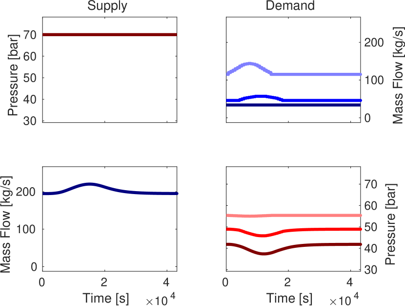
(a) Hypothetical network’s test scenario.

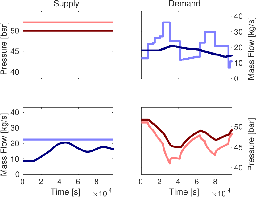
(b) Actual network’s test scenario.

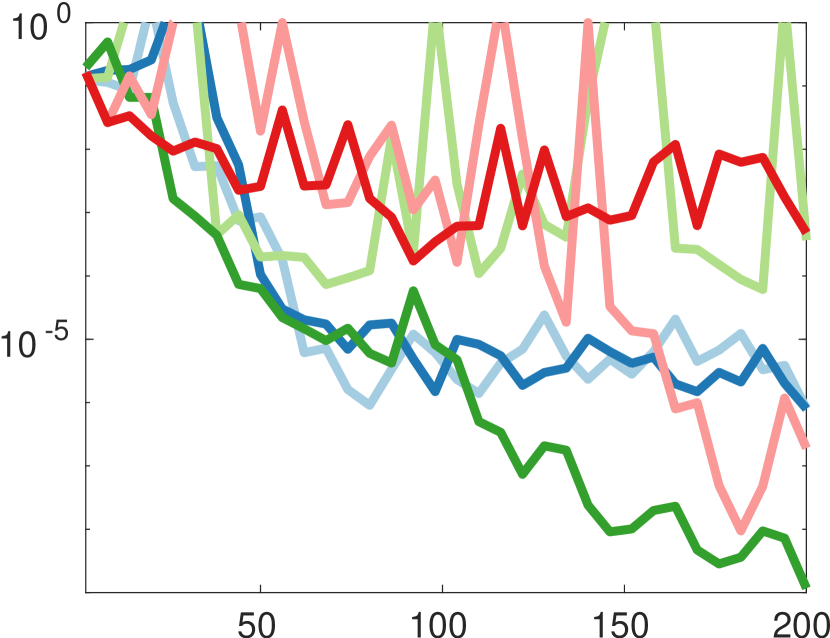
(c) Relative $L_{2}\otimes L_{2}$ error between ROM and FOM for the ode_end model, imex1 solver, and linear reductors versus reduced order for the hypothetical network.

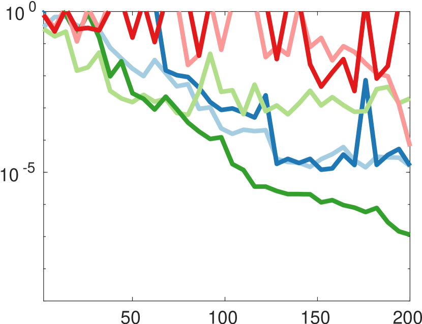
(d) Relative $L_{2}\,\otimes\,L_{2}$ error between ROM and FOM for the ode_end model, imex1 solver, and linear reductors versus reduced order for the actual network.

(e) Common legend for the model reduction error plots.

Reductor	MORscore	Avg. Gain Error
pod_r	$0.27$	$6\cdot 10^{-6}$
gopod_r	$0.26$	$6\cdot 10^{-6}$
dmd_r	$0.18$	$8\cdot 10^{-6}$
eds_ro_l	$0.30$	$8\cdot 10^{-6}$
eds_wx_l	$0.18$	$8\cdot 10^{-6}$
eds_wz_l	$0.15$	$8\cdot 10^{-6}$

(f) MORscores $\mu(200,\epsilon_{\operatorname{mach}(16)})$ in the $L_{2}\otimes L_{2}$ error norm, and mean steady-state gain error for the hypothetical network.

Reductor	MORscore	Avg. Gain Error
pod_r	$0.19$	$2\cdot 10^{-5}$
gopod_r	$0.15$	$1\cdot 10^{-5}$
dmd_r	$0.15$	$2\cdot 10^{-5}$
eds_ro_l	$0.24$	$2\cdot 10^{-5}$
eds_wx_l	$0.04$	$2\cdot 10^{-5}$
eds_wz_l	$0.03$	$2\cdot 10^{-5}$

(g) MORscores $\mu(200,\epsilon_{\operatorname{mach}(16)})$ in the $L_{2}\otimes L_{2}$ error norm, and mean steady-state gain error for the actual network.

Figure 1: Visualization of the test scenario, model reduction errors, MORscores, and gain errors of the tested ROMs for the hypothetical network [5, Part 2] (left side) and actual network [5, Part 3] (right side). Computed with MATLAB 2021a.

4 Next-Gen Gas Network Simulation

Based on the heuristic comparison in [3] and this work’s numerical results, we recommend a port-Hamiltonian model, an implicit-explicit solver, and a Galerkin reductor, particularly, the endpoint discretization, the first order IMEX time stepper, and the structured empirical dominant subspaces method as the model-solver-reductor ensemble, for the next generation of transient gas network simulators.

References

- [1] G. Bachman and M. Goodreau. Less is more accuracy versus precision in modeling. In PSIG Annual Meeting 2000, pages PSIG–0009, 2000. URL: https://onepetro.org/PSIGAM/proceedings-abstract/PSIG00/All-PSIG00/PSIG-0009/2043.
- [2] M. Behbahani-Nejad, A. Bermúdez, and M. Shabani. Finite element solution of a new formulation for gas flow in a pipe with source terms. Journal of Natural Gas Science and Engineering, 61:237–250, 2019. doi:10.1016/j.jngse.2018.11.019.
- [3] C. Himpe, S. Grundel, and P. Benner. Model order reduction for gas and energy networks. Journal of Mathematics in Industry, 11:13, 2021. doi:10.1186/s13362-021-00109-4.
- [4] A. Lewandowski. New numerical methods for transient modeling of gas pipeline networks. In PSIG Annual Meeting, pages PSIG–9510, 1995. URL: https://onepetro.org/PSIGAM/proceedings-abstract/PSIG95/All-PSIG95/PSIG-9510/2571.
- [5] L. A. Lotito and P. W. Halbert. Computer simulation of gas flow dynamics. Pipeline Engineer, 39:31–33, 29–31, 45–47, 1967.
- [6] J. L. Mead and R. A. Renaut. Optimal Runge-Kutta methods for first order pseudospectral operators. Journal of Computational Physics, 152(1):404–419, 1999. doi:10.1006/jcph.1999.6260.
- [7] R. Samar, I. Postlewaite, and D. W. Gu. Model reduction with balanced realizations. Internat. J. Control, 62(1):33–64, 1995. doi:10.1080/00207179508921533.
- [8] W. Q. Tao and H. C. Ti. Transient analysis of gas pipeline network. Chemical Engineering Journal, 69(1):47–52, 1998. doi:10.1016/S1385-8947(97)00109-5.
- [9] P. J. van der Houwen. Explicit Runge-Kutta formulas with increased stability boundaries. Numerische Mathematik, 20:149–164, 1972. doi:10.1007/BF01404404.
- [10] A. van der Schaft. Interconnections of input-output Hamiltonian systems with dissipation. In Proceedings of the 55th IEEE Conference on Decision and Control, pages 4886–4691, 2016. doi:10.1109/CDC.2016.7798983.