Online Hashing with Similarity Learning

Abstract

Online hashing methods usually learn the hash functions online, aiming to efficiently adapt to the data variations in the streaming environment. However, when the hash functions are updated, the binary codes for the whole database have to be updated to be consistent with the hash functions, resulting in the inefficiency in the online image retrieval process. In this paper, we propose a novel online hashing framework without updating binary codes. In the proposed framework, the hash functions are fixed and a parametric similarity function for the binary codes is learnt online to adapt to the streaming data. Specifically, a parametric similarity function that has a bilinear form is adopted and a metric learning algorithm is proposed to learn the similarity function online based on the characteristics of the hashing methods. The experiments on two multi-label image datasets show that our method is competitive or outperforms the state-of-the-art online hashing methods in terms of both accuracy and efficiency for multi-label image retrieval.

Introduction

The large amount of visual data (e.g. images and videos) that is produced everyday leads to the development of efficient index and retrieval methods. Among these methods, hashing methods that perform approximate nearest neighbor search by mapping high-dimensional data to binary codes have attracted increasing attention (Wang et al. 2016, 2018).

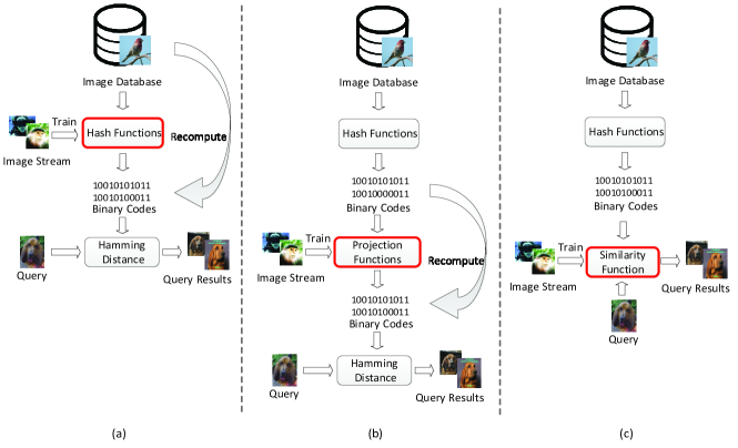
Figure 1: Comparison of online hashing frameworks. (a) The framework updates the hash functions and recomputes the binary codes. (b) The framework updates the projections functions and projects the binary codes. (c) The framework updates the similarity function without updating binary codes.

Locality Sensitive Hashing (LSH) (Andoni and Indyk 2006) is a representative of the hashing methods. By generating as hash functions random projection vectors sampled from a multidimensional Gaussian distribution with zero mean and identity covariance matrix, LSH can hash similar data into similar binary codes in a high probability. However, LSH is a data-independent hashing method and usually needs long binary codes to achieve a good precision. To obtain compact binary codes for the data, data-dependent hashing methods (Weiss, Torralba, and Fergus 2009; Weiss, Fergus, and Torralba 2012; He, Wang, and Cheng 2019; Weng and Zhu 2020a) employ machine learning techniques to learn the hash functions according to the data. For example, some hashing methods (Ge, He, and Sun 2014; Liu et al. 2014; Li, Hu, and Nie 2017) build graphs to describe the relationship between the data and learn the hash functions from the graphs. Some hashing methods (Gong et al. 2013; He, Wen, and Sun 2013) adopt dimensionality reduction techniques to project the data into a low-dimensional space and quantize each dimension into a bit. Due to the development of deep learning methods, deep hashing methods (Shen et al. 2018; Do, Doan, and Cheung 2016; Cao et al. 2018; Wu et al. 2019) learn the neural networks as the hash functions. Since the memory space is limited, deep hashing methods learn the hash functions by using minibatch-based stochastic optimization which requires multiple passes over a given database. Although these methods can achieve good search performance, they are designed for the static database and have poor scalability for the ever-growing database. When new data arrives, the hash functions have to be re-learnt by accumulating all the training data, which is time-consuming.

To address this challenge, online hashing methods (Lin et al. 2019; Cakir et al. 2017; Lin et al. 2020b, 2018a; Weng et al. 2019) employ online learning techniques to learn the hash functions online from the streaming data. For example, Online Sketching Hashing (OSH) (Leng et al. 2015) maintains a small-size data sketch from the streaming data and learns hash functions from the data sketch. Online Kernel Hashing (OKH) (Huang, Yang, and Zheng 2018) constructs a loss function by using the label information and updates the hash functions according to the loss function. Balanced Similarity for Online Discrete Hashing (BSODH) (Lin et al. 2019) uses an asymmetric graph regularization to preserve the similarity between the streaming data and the existing dataset and update the hash function according to the graph. Online Supervised Hashing (OSupH) (Cakir, Bargal, and Sclaroff 2017) and Hadamard Matrix Guided Online Hashing (HMOH) (Lin et al. 2020a) explore how to generate the target codes according to the label information and update the hash functions according to the target codes. Although the current online hashing methods can achieve good search performance and are efficient in learning the hash functions online, they have to recompute the binary codes for the database when the hash functions are updated. It is inefficient since recomputing the binary codes needs to accumulate the whole database as shown in Fig. 1(a). Mutual Information Hashing (MIH) (Cakir et al. 2017) has noticed this problem and introduces a trigger update module to reduce the frequency of recomputing the binary codes, but the calculation in the trigger update module is time-consuming (Weng and Zhu 2020d). Online Hashing with Efficient Updating (OHWEU) (Weng and Zhu 2020d) tries to solve this problem from another perspective. It designs an online hashing framework that fixes the hash functions and learns the projection functions online to project the binary codes into another binary space. Hence, OHWEU can update the binary codes efficiently without accumulating the whole database, which is shown in Fig. 1(b). However, for OHWEU, the cost of updating the binary codes is increasing as data is growing.

In this paper, we propose a new online hashing framework without updating binary codes. In this framework, we fix the hash functions and introduce a similarity function to measure the similarity between the query and the binary codes. And the similarity function is learnt online from the streaming data to adapt to the data variations. Fig. 1 shows the difference between our framework (Fig. 1(c)) and other online hashing frameworks. Compared with the other two online hashing framework, our framework omits the process of updating the binary codes, which is efficient for the ever-growing data. Our contribution in this paper is three fold:

• A novel online hashing framework without updating binary codes is proposed by introducing a parametric similarity function that is learnt online from the streaming data.

• A new online metric learning algorithm is proposed to learn the similarity function that has a bilinear form, which can treat the query and the binary codes asymmetrically.

• The experiments on two multi-label datesets show that our method not only achieves competitive or higher search accuracy than other online hashing methods but also is more efficient in the online process.

Related Work

Hashing methods with similarity functions

Since Hamming distance has a limited distance range and easily causes the ambiguity problem, some emerging studies (Ji et al. 2014; Zhang et al. 2013; Duan et al. 2015; Zhang and Peng 2018) explore using other similarity functions to measure the similarity between binary codes rather than Hamming distance. For example, Manhattan Hashing (Kong, Li, and Guo 2012) uses Manhattan distance to replace Hamming distance as Manhattan distance can preserve more information about the neighborhood structure in the original feature than Hamming distance. And some studies (Duan et al. 2015; Zhang and Peng 2018; Weng et al. 2016) adopt weighted Hamming distance to replace Hamming distance and allocate the weights to each bit.

Although Manhattan distance and weighted Hamming distance can provide superior accuracy than Hamming distance, the computation of Manhattan distance and weighted Hamming distance is slower than that of Hamming distance as the search with Hamming distance can be accelerated in a non-exhaustive search way which can provide a sub-linear search time. To solve this problem, recently, Multi-Index Weighted Querying (MIWQ) (Weng and Zhu 2020b) develops a non-exhaustive search method to accelerate the search with weighted Hamming distance, propelling the development of the hashing methods with weighted Hamming distance.

In this paper, our method uses a bilinear similarity function to replace Hamming distance since the similarity function can be learnt in an online way to adapt to the data variations in the streaming environment. Meanwhile, the computation of the bilinear similarity between the binary codes can be represented in a form of weighted Hamming distance, so that it can be accelerated by MIWQ.

Metric learning methods

Metric learning methods (Kulis et al. 2012; Wang and Sun 2015) aim to learn a similarity function tuned to a particular task and are widely used in different applications that rely on distances or similarities. In terms of learning methodology, metric learning methods can be categorized as batch-based learning methods (Wang et al. 2017; Cakir et al. 2019) and online learning methods (Gao et al. 2017; Chechik et al. 2010).

Our method follows the online-learning methodology. Our method is related to LogDet Exact Gradient Online (LEGO) (Jain et al. 2009) which applies online metric learning technique on updating the hash functions generated by LSH. However, in LEGO, the binary codes need to be recomputed when the hash functions are updated, which is the main difference between LEGO and our method.

Online Hashing with Similarity Learning

Similarity function

Hashing methods learn the hash functions to map a $D$-dimensional feature vector ${\bf{x}}\in{{\mathbb{R}}^{D}}$ to a $b$-bit binary hash code ${\bf{\tilde{x}}}\in{\{-1,1\}^{b}}$. Given a query ${\bf{q}}\in{{\mathbb{R}}^{D}}$, the query $\mathbb{q}$ is hashed into a binary hash code $\mathbb{\tilde{q}}\in{\{-1,1\}^{b}}$ and Hamming distance between the binary query $\mathbb{\tilde{q}}$ and the binary code ${\bf{\tilde{x}}}$ is calculated as

$${S_{H}}({\bf{\tilde{q}}},{\bf{\tilde{x}}})=\sum\limits_{i=1}^{b}{{{\tilde{q}}_{i}}\otimes{{\tilde{x}}_{i}}},$$ (1)

where $\otimes$ is an xor operation.

We consider a parametric similarity function that has a bilinear form to replace Hamming distance, which is,

$${S_{{\bf{\tilde{M}}}}}({\bf{\tilde{q}}},{\bf{\tilde{x}}})={{\bf{\tilde{q}}}^{T}}{\bf{\tilde{M}\tilde{x}}},$$ (2)

where ${\bf{\tilde{M}}}\in{\mathbb{R}}^{b\times b}$.

There are two advantages to use the bilinear similarity: (a) It can avoid imposing positivity or square constraints that result in computationally intensive solutions. (b) It can be combined with MIWQ (Weng and Zhu 2020b) to accelerate the search process. These two advantages are elaborated in the following.

In (Neyshabur et al. 2013; Weng and Zhu 2020d), it shows that treating the queries and the database points asymmetrically can improve the search accuracy. In detail, although the database points are hashed into binary codes, the query does not need to be hashed into a binary code so that more information of the query can be preserved. Hence, we treat the query points and the database points in an asymmetric way by modifying Eqn. (2) as

$${S_{\bf{M}}}({\bf{q}},{\bf{\tilde{x}}})={{\bf{q}}^{T}}{\bf{M\tilde{x}}},$$ (3)

where ${\bf{M}}\in{\mathbb{R}}^{D\times b}$, $\bf q$ is the original feature vector and is not mapped to a binary code.

Since the query is fixed in each comparison between the query and the binary codes in the process of searching for the nearest neighbors of the query, the multiplication between q and M can be pre-computed and stored. Hence, Eqn. (3) is rewritten as

$${S_{\bf{M}}}({\bf{q}},{\bf{\tilde{x}}})={{\bf{\hat{m}}}^{T}}{\bf{\tilde{x}}},$$ (4)

where ${\bf{\hat{m}}}={({{\bf{q}}^{T}}{\bf{M}})^{T}}$.

Further, Eqn. (4) can be rewritten as a form of weighted Hamming distance

$${S_{\bf{M}}}({\bf{q}},{\bf{\tilde{x}}})=\sum\limits_{i=1}^{b}{{w_{i}}({{\tilde{x}}_{i}})},$$ (5)

where ${\tilde{x}}_{i}$ is the $i^{th}$ bit of $\bf{\tilde{x}}$, ${w_{i}}:\{-1,1\}\to{\mathbb{R}}$ is a function to store the pre-computed value for the $i^{th}$ bit and is defined as

$$\left\{\begin{array}[]{l}{w_{i}}(-1)=-{{\hat{m}}_{i}}\\ {w_{i}}(1)={{\hat{m}}_{i}}.\end{array}\right.$$ (6)

and ${{\hat{m}}_{i}}$ is the $i^{th}$ element of ${\bf{\hat{m}}}$.

Since the computation of the similarity function in Eqn. (3) can be rewritten as a form of weighted Hamming distance Eqn. (5), it can be combined with MIWQ (Weng and Zhu 2020b) to perform the non-exhaustive search with the learnt similarity when given a query. In (Weng and Zhu 2020b), it shows that the non-exhaustive search with weighted Hamming distance is competitive to the search with Hamming distance for the compact binary codes in terms of search efficiency. More details of MIWQ can be seen in (Weng and Zhu 2020b).

In our framework, the hash functions are learnt in advance and fixed. Following other online hashing methods, the linear projection-based hash functions are adopted, which are

$${\bf{\tilde{x}}}={\mathop{\rm sgn}}({{\bf{W}}^{T}}{\bf{x}}+{\bf{b}}),$$ (7)

where $\mathbb{W}\in{\mathbb{R}}^{D\times b}$ is a projection matrix and $\mathbb{b}\in{\mathbb{R}}^{b}$ is a threshold vector.

As (Huang, Yang, and Zheng 2018; Weng and Zhu 2020d) do, by assuming there is a small amount of training data in the initial stage, we can use the training data to learn the hash functions that can preserve the data similarity in the initial stage. Here, we learn the hash functions by using Iterative Quantization (PCA-ITQ) (Gong et al. 2013) which is an unsupervised hashing method to preserve the similarity between data effectively for both the seen and the unseen data. It is justified in (Li, Liu, and Huang 2018) that the hash functions can be learnt by PCA-ITQ just with a small amount of training data.

Online learning

Although Online Algorithm for Scalable Image Similarity learning (OASIS) (Chechik et al. 2009, 2010) provides a solution for learning the similarity matrix $\mathbb{M}$ in Eqn. (3), the similarity matrix $\mathbb{M}$ in OASIS is a square matrix while it can be a rectangular matrix in our method. Hence, we propose a new online metric learning algorithm to learn the similarity matrix.

The similarity matrix $\bf{M}$ in Eqn. (3) can be decomposed as

$$\mathbb{M}=\mathbb{U}^{T}\mathbb{V}$$ (8)

where $\mathbb{U}\in{\mathbb{R}}^{l\times D}$ and $\mathbb{V}\in{\mathbb{R}}^{l\times b}$ are linear transformation.

Therefore, Eqn. (3) can be rewritten as

$${S_{\bf{M}}}({\bf{q}},{\bf{\tilde{x}}})={{\bf{q}}^{T}}{\bf{M\tilde{x}}}={{\bf{q}}^{T}}{{\bf{U}}^{T}}{\bf{V\tilde{x}}}={({\bf{Uq}})^{T}}{\bf{V\tilde{x}}}.$$ (9)

The similarity between $\bf{q}$ and $\mathbb{\tilde{x}}$ can be treated as the inner product of two vectors ${\bf{Uq}}$ and ${\bf{V\tilde{x}}}$ . If two data points are similar, the inner product of their corresponding vectors after linear transformation should be larger than that of dissimilar ones. To learn the similarity function using the point-wise label information, inspired by HMOH (Lin et al. 2020a), we can generate $l$-bit binary target code ${\bf{g}}\in{\{-1,1\}^{l}}$ according to the label information so that each column $\mathbb{u}\in{\mathbb{R}}^{D}$ in $\mathbb{U}$ is a projection vector and corresponds to one bit of the binary target code. So is each column $\mathbb{v}\in{\mathbb{R}}^{b}$ in $\mathbb{V}$. This idea is shown in Fig. 2.

It should be noted that the length $l$ of the binary target code ${\bf{g}}$ will affect the performance of our method. When $l$ increases, the search accuracy of our method usually improves in the case of low bits. Considering about the constraint of the rank of $\bf M$ and the learning efficiency, we take $l=3b$ ($i.e.$, the binary target code is three times the length of the generated binary hash codes) which will be demonstrated in the experiments.

Generating the $l$-bit binary target codes that can preserve the label information has been explored in some online hashing methods (Cakir, Bargal, and Sclaroff 2017; Weng and Zhu 2020c; Lin et al. 2020a, 2018b). Here, we adopt HMOH (Lin et al. 2020a) to introduce the Hadamard matrix and regard each column of Hadamard matrix as the binary target code ${\bf{g}}\in{\{-1,1\}^{l}}$ for each class label, which by nature satisfies several desired properties of binary hash codes.

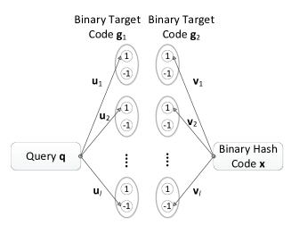
Figure 2: An example of learning projection vectors.

As shown in Fig. 2, after obtaining the binary target codes according to the label information, each projection vector $\bf u$ in $\bf U$ can be learnt online as an online binary classification problem. We adopt the Passive-Aggressive algorithm (Crammer et al. 2006) to learn the projection vector as it can converge to a high quality projection vector after learning from a small amount of training data.

When a data point $\bf x$ with its binary target code $\bf g$ arrives, for each projection vector $\bf u$ and its corresponding bit $g$ in the binary target code $\bf g$, the hinge-loss function is defined as

$$\ell({\bf{u}};({\bf{x}},g))=\left\{\begin{array}[]{l}0\quad\quad\quad\quad\quad\quad\;g({{\bf{u}}^{T}}{\bf{x}})\geq 1\\ 1-g({{\bf{u}}^{T}}{\bf{x}})\;\;\,\quad otherwise.\end{array}\right.$$ (10)

For brevity, we use $\ell_{i}$ to represent $\ell({\bf{u}};({{\bf{x}}_{i}},{g_{i}}))$ where $\mathbb{x}_{i}$ is the data point and $g_{i}$ is the corresponding bit of the binary target code $\mathbb{g}_{i}$ in the $i^{th}$ round. At first, $\bf u$ is initialized to a zero-valued vector. Then, for each round $i$, we solve the following convex problem with soft margin:

$$\begin{array}[]{l}{{\bf{u}}_{i}}=\mathop{\arg\;\min}\limits_{\bf{u}}\;{\textstyle{1\over 2}}||{\bf{u}}-{{\bf{u}}_{i-1}}|{|^{2}}+C\xi\\ s.t.\quad{\ell_{i}}\leq\xi\;and\;\xi\geq 0\end{array}$$ (11)

where $||\cdot||$ is the Euclidean norm and $C$ controls the trade-off between making $\bf u$ stay close to the previous parameter $\mathbb{u}_{i-1}$ and minimizing the loss on the current loss $\ell_{i}$.

When $\ell_{i}$ = 0, $\mathbb{u}_{i}=\mathbb{u}_{i-1}$ satisfies Eqn.(11) directly. Otherwise, we define the Lagrangian as:

$$L(\bf{p},\tau,\lambda,\xi)={\textstyle{1\over 2}}||{\bf{p}}-{{\bf{p}}_{i-1}}||^{2}+C\xi+\tau(1-\xi-{g_{i}^{*}}({{\bf{p}}^{T}}{{\bf{h}}_{i}}))-\lambda\xi,$$ (12)

with $\tau\geq 0$ and $\lambda\geq 0$ are Lagrange multipliers.

Let $\frac{{\partial L({\bf{u}},\tau,\lambda,\xi)}}{{\partial{\bf{u}}}}={\bf{u}}-{{\bf{u}}_{i-1}}-\tau{g_{i}}{{\bf{x}}_{i}}=0$, we obtain

$${\bf{u}}={{\bf{u}}_{i-1}}+\tau{g_{i}}{{\bf{x}}_{i}}.$$ (13)

Let $\frac{{\partial L({\bf{u}},\tau,\lambda,\xi)}}{{\partial\xi}}=C-\tau-\lambda=0$, we obtain

$$C=\tau+\lambda,$$ (14)

where $\tau\leq C$ as $\lambda\geq 0$

Plugging Eqn. (14) and (15) back into Eqn. (12), we obtain $L(\tau)=-{\textstyle{1\over 2}}{\tau^{2}}||{{\bf{x}}_{i}}|{|^{2}}+\tau(1-{g_{i}}({\bf{u}}_{i-1}^{T}{{\bf{x}}_{i}}))$. Let $\frac{{\partial L(\tau)}}{{\partial\tau}}=-\tau||{{\bf{x}}_{i}}|{|^{2}}+(1-{g_{i}}({\bf{u}}_{i-1}^{T}{{\bf{x}}_{i}}))=0$, we obtain

$$\tau=\frac{{1-{g_{i}}({\bf{u}}_{i-1}^{T}{{\bf{x}}_{i}})}}{{||{{\bf{x}}_{i}}||}}.$$ (15)

Therefore, the solution to Eqn. (11) is

$${{\bf{u}}_{i}}={{\bf{u}}_{i-1}}+\tau{g_{i}}{{\bf{x}}_{i}},$$ (16)

where

$$\tau=\min\{C,\frac{{1-{g_{i}}({\bf{u}}_{i-1}^{T}{{\bf{x}}_{i}})}}{{||{{\bf{x}}_{i}}||}}\}.$$ (17)

Similarly, for each projection vector $\mathbb{v}$, the data point $\bf x$ is hashed into a binary hash code $\bf\tilde{x}$ by hash functions in Eqn. (7), and the hinge-loss function is defined as

$$\tilde{\ell}({\bf{v}};({\bf{\tilde{x}}},g))=\left\{\begin{array}[]{l}0\quad\quad\quad\quad\quad\quad\;g({{\bf{v}}^{T}}{\bf{\tilde{x}}})\geq 1\\ 1-g({{\bf{v}}^{T}}{\bf{\tilde{x}}})\quad\;\;\,otherwise.\end{array}\right.$$ (18)

For brevity, we use $\tilde{\ell}_{i}$ to represent $\tilde{\ell}({\bf{v}};({\bf{\tilde{x}_{i}}},g_{i}))$. At first, $\bf v$ is initialized to a zero-valued vector. Then, for each round $i$, we solve the following convex problem with soft margin:

$$\begin{array}[]{l}{{\bf{v}}_{i}}=\mathop{\arg\;\min}\limits_{\bf{v}}\;{\textstyle{1\over 2}}||{\bf{v}}-{{\bf{v}}_{i-1}}|{|^{2}}+C\xi\\ s.t.\quad{\tilde{\ell}_{i}}\leq\xi\;and\;\xi\geq 0.\end{array}$$ (19)

Following the above derivation, the solution to Eqn. (19) is

$${{\bf{v}}_{i}}={{\bf{v}}_{i-1}}+\tau{g_{i}}{{\bf{\tilde{x}}}_{i}},$$ (20)

where

$$\tau=\min\{C,\frac{{1-{g_{i}}({\bf{v}}_{i-1}^{T}{{\bf{\tilde{x}}}_{i}})}}{{||{{\bf{\tilde{x}}}_{i}}||}}\}.$$ (21)

The pseudo-code of our method, Online Hashing with Similarity Learning (OHSL), is summarized in Algorithm 1.

Algorithm 1 OHSL

0:  streaming data $(\mathbb{x}_{i},\mathbb{y}_{i})$, parameters $C$ and $l$

0:  $\mathbb{M}$

1:  Initialize $\mathbb{U}=[0,...,0]$ and $\mathbb{V}=[0,...,0]$

2:  for $i=1,2,...$ do

3:     Obtain the binary target code $\mathbb{g}_{i}$ following HMOH

4:     for each $\bf u$ in $\bf U$ do

5:        Update $\bf u$ by Eqn. (16)

6:     end for

7:     Obtain the binary representation $\mathbb{\tilde{x}}_{i}$ by Eqn.(7)

8:     for each $\bf v$ in $\bf V$ do

9:        Update $\bf v$ by Eqn. (20)

10:     end for

11:     $\mathbb{M}=\mathbb{U}^{T}\mathbb{V}$

12:  end for

Experiments

Datasets

The following experiments are performed on two commonly-used multi-label image datasets, MS-COCO and NUS-WIDE.

(a).MS-COCO dataset (Lin et al. 2014). The MS-COCO dataset is a multi-label dataset including training images and validation images. Each image is labeled by some of the 80 concepts. After filtering out the images that do not contain any concept label, there are 122,218 images left. Each images is represented by a 4096-D feature extracted from the fc7 layer of a VGG-16 network (Simonyan and Zisserman 2014) pretrained on ImageNet (Deng et al. 2009). For each category, we randomly take 50 images as the query images and the rest as the database images.

(b). NUS-WIDE dataset (Chua et al. 2009). The NUS-WIDE dataset is a multi-label dataset including 269,648 web images associated with tags. Following (Kang, Li, and Zhou 2016), the images that belong to the 21 most frequent concepts are selected and there are 195,834 images left. Each images is represented by a 4096-D feature extracted from the fc7 layer of a VGG-16 network (Simonyan and Zisserman 2014) pretrained on ImageNet. For each category, we randomly take 50 images as the query images and the rest as the database images.

Table 1: The mAP results on MS-COCO. The best result is labeled with boldface and the second best has an underline.

	mAP
	16 bits	32 bits	64 bits	96 bits
$\mathbb{OHSL}$	$\mathbb{0.524}$	$\mathbb{0.536}$	$\mathbb{0.574}$	$\mathbb{0.578}$
OHWEU	0.444	0.506	0.539	0.567
HMOH	0.460	0.501	0.534	0.550
MIH	0.442	0.435	0.438	0.488
OSupH	0.463	0.495	0.512	0.514
OKH	0.412	0.436	0.470	0.484
BSODH	0.458	0.437	0.434	0.431
OSH	0.457	0.483	0.499	0.504

Table 2: The mAP results on NUS-WIDE. The best result is labeled with boldface and the second best has an underline.

	mAP
	16 bits	32 bits	64 bits	96 bits
$\mathbb{OHSL}$	0.667	0.673	0.700	0.701
OHWEU	0.552	0.637	0.653	0.670
HMOH	$\mathbb{0.668}$	$\mathbb{0.716}$	$\mathbb{0.725}$	$\mathbb{0.728}$
MIH	0.571	0.635	0.649	0.647
OSupH	0.611	0.612	0.631	0.640
OKH	0.506	0.550	0.555	0.598
BSODH	0.614	0.611	0.613	0.620
OSH	0.466	0.489	0.514	0.522

Accuracy comparison

Following (Cakir et al. 2017; Lin et al. 2019), mean Average Precision (mAP) is used to measure the search accuracy of the online hashing methods. If the images and the query share at least one common label, they are defined as a groundtruth neighbor. The results are averaged by repeating the experiments 10 times.

We compare our method, OHSL, with OHWEU (Weng and Zhu 2020d), HMOH (Lin et al. 2020a), BSODH (Lin et al. 2019), MIH (Cakir et al. 2017), OSupH (Cakir, Bargal, and Sclaroff 2017), OKH (Huang, Yang, and Zheng 2018) and OSH (Leng et al. 2015). The key parameters in each compared method are set as the ones recommended in the corresponding papers except a small amount of parameters are adjusted to be suitable for the datasets. In MIH, the reservoir size is set to 200 to make a good tradeoff between the accuracy and the training cost. Following the operation in OKH and OHWEU, we take 300 data points to train the hash functions in the initial stage.

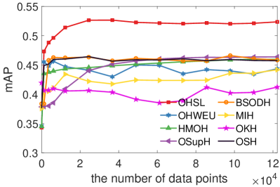
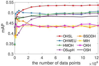
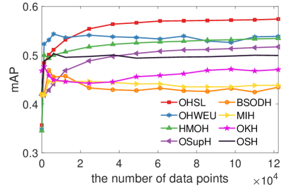
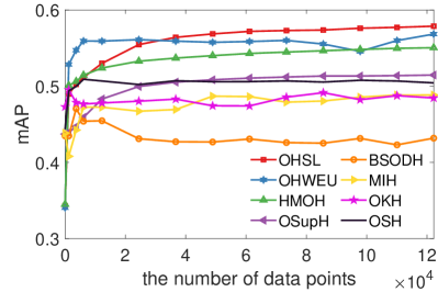
(a) 16 bits	(b) 32 bits	(c) 64 bits	(d) 96 bits

Figure 3: The mAP results of different online hashing methods with training data increasing on MS-COCO.

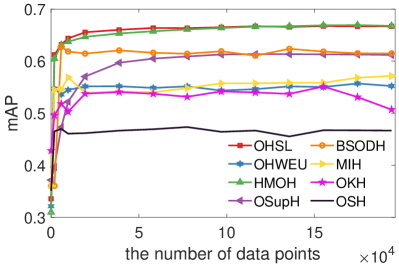
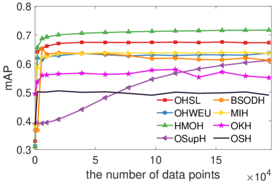
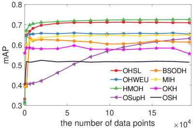
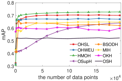
(a) 16 bits	(b) 32 bits	(c) 64 bits	(d) 96 bits

Figure 4: The mAP results of different online hashing methods with training data increasing on NUS-WIDE.

Table 1 and Table 2 show the mAP results of different online hashing methods on MS-COCO and NUS-WIDE, respectively. The best results are bolded and the second results are underlined. On MS-COCO, OHSL can achieve the best results among the online hashing methods and OHWEU achieves the second best results in most of the cases. On NUS-WIDE, HMOH achieves the best results among the online hashing methods and OHSL achieves the second best results.

Fig. 3 shows the mAP results of different online hashing methods with the training data increasing from 16 bits to 96 bits on MS-COCO. From 16 bits to 64 bits, OHSL can achieve the better mAP results than other online hashing methods after taking only a few training data for training. For 96 bits, OHWEU can achieve the better mAP results than other online hashing methods after taking only a few training data for training at first. With the data increasing, OHSL is better than OHWEU.

Fig. 4 shows the mAP results of different online hashing methods with the training data increasing from 16 bits to 96 bits on NUS-WIDE. From 16 bits to 96 bits, OHSL and HMOH can achieve the better mAP results than other online hashing methods after taking only a few training data for training. And HMOH is better than OHSL.

Efficiency comparison

To compare the efficiency of different online hashing methods, we calculate the time cost by running the experiments on a PC with Intel i7 3.4 GHz CPU, 24 GB memory. Assume the data comes in chunks (Leng et al. 2015) and each chunk is composed of 1000 data points. The online hashing methods update the functions when receiving one chunk of data.

Fig. 5 shows the accumulated time cost of different online hashing methods with the data samples increasing on NUS-WIDE for 32 bits. ’IO’ denotes the time cost of accumulating all the received data for computing the binary codes by exchanging the data between the hard disk and RAM. The exchanging operation is implemented by C++ code. It takes 3.97s to transfer 1000 4096-D data points from the hard disk to RAM averagely. For IO, the accumulated time cost rises as a quadratic function of the number of data. For HMOH, OSupH and OSH, the accumulated time cost also rises as a quadratic function of the number of data since they need to take into account the time cost of IO which takes a majority in the total time cost. For MIH, the time cost is approximately linear to the data size since it adopts the trigger update module to reduce the frequency of recomputing the binary codes. However, its time cost is still high due to the time-consuming computations in the trigger update module. Compared with IO, OHSL and OHWEU are much faster, which implicitly denotes that the time cost of exchanging the data is much larger than the time cost of updating the binary codes and learning the functions online. By zooming in the comparison among OHSL and OHWEU, we can see that the accumulated time cost of OHWEU also rises as a quadratic function of the number of data while the accumulated time cost of OHSL is linear to the data size. OHWEU need to update the binary codes once the projection functions are updated and the time cost of each updating operation is linear to the data size. The accumulated time cost of OHWEU rises as a quadratic function of the data size as the accumulated time cost adds up the time cost of each updating operation.

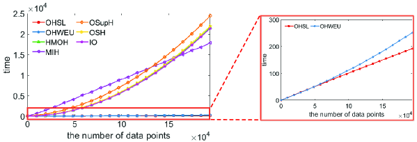
Figure 5: The accumulated time cost of different online hashing methods with data increasing on NUS-WIDE.

Parameter analysis

There are two key parameters $C$ and $l$ in our method and we investigate the influence of these parameters.

By setting the length of the binary target code is equal to the bit number, $i.e.,$ $l=b$, we investigate the influence of the parameter $C$. Fig. 6 shows the comparison of OHSL by using different parameter values of $C$. As denoted in Eqn. (11) and (19), $C$ controls the trade-off between making the projection vector stay close to the previous vector and minimizing the current loss. Both $C$ in Eqn. (11) and (19) choose the same value. According to the results, the best parameter choice on MS-COCO and NUS-WIDE is $C=0.01$.

By setting $C=0.01$, we investigate the influence of the parameter $l$. Fig. 7 shows the comparison of OHSL by using different parameter values of $l$, where 1x denotes $l=b$ ($i.e.,$ the length of the binary target code is equal to the bit number), 2x denotes $l=2b$, 3x denotes $l=3b$ and 4x denotes $l=4b$. With the increase of the length of the binary target code $l$, our method can achieve better accuracy. Although the accuracy is improved as the length of the binary target code increases, its time cost also rises. As the accuracy and the time cost are both important, to achieve a good balance between the accuracy and the time cost, we take $l=3b$.

Fig. 8 shows the comparison by using different ways to learn the bilinear similarity function. OHSL-sym denotes our method process the query and the binary codes symmetrically as shown in Eqn. (2). OASIS (Chechik et al. 2010) and LEGO (Jain et al. 2009) are the classical online metric learning methods to learn the square bilinear similarity by taking the binary codes as the input. By comparing OHSL to OHSL-sym, it shows that process the query and the binary codes asymmetrically can boost the search accuracy. And our method can achieve better accuracy than OASIS and LEGO.

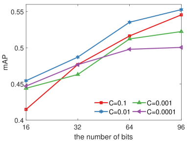
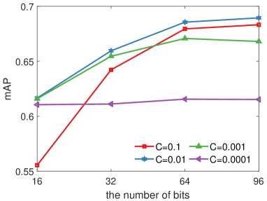
(a) MS-COCO	(b) NUS-WIDE

Figure 6: The mAP results of different $C$.

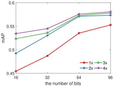
(a) MS-COCO	(b) NUS-WIDE

Figure 7: The mAP results of different $l$.

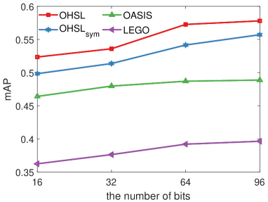
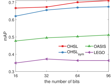
(a) MS-COCO	(b) NUS-WIDE

Figure 8: The mAP results of different online learning ways.

Conclusions

In this paper, we propose a new online hashing framework without updating binary codes. By introducing the bilinear similarity function, the process of updating binary codes is omitted and the similarity function is learnt online to adapt to the streaming data. A metric learning algorithm is proposed to learn the similarity function that can treat the query and the binary codes asymmetrically. The experiments on two multi-label datasets show that compared with the online hashing methods that need to update the hash functions, our method can achieve competitive or better search accuracy with much smaller time cost. Compared with the online hashing method that fixes the hash functions and learns the projection functions, our method outperforms it in terms of efficiency and accuracy.

References

- Andoni and Indyk [2006] Andoni, A.; and Indyk, P. 2006. Near-optimal hashing algorithms for approximate nearest neighbor in high dimensions. In 47th Annual IEEE Symposium on Foundations of Computer Science, 459–468.
- Cakir, Bargal, and Sclaroff [2017] Cakir, F.; Bargal, S. A.; and Sclaroff, S. 2017. Online supervised hashing. Computer Vision and Image Understanding 156: 162–173.
- Cakir et al. [2017] Cakir, F.; He, K.; Bargal, S. A.; and Sclaroff, S. 2017. MIHash: Online Hashing with Mutual Information. In Proceedings of the IEEE International Conference on Computer Vision, 437–445.
- Cakir et al. [2019] Cakir, F.; He, K.; Xia, X.; Kulis, B.; and Sclaroff, S. 2019. Deep metric learning to rank. In Proceedings of the IEEE Conference on Computer Vision and Pattern Recognition, 1861–1870.
- Cao et al. [2018] Cao, Y.; Long, M.; Liu, B.; Wang, J.; and KLiss, M. 2018. Deep Cauchy Hashing for Hamming Space Retrieval. In Proceedings of the IEEE Conference on Computer Vision and Pattern Recognition, 1229–1237.
- Chechik et al. [2009] Chechik, G.; Shalit, U.; Sharma, V.; and Bengio, S. 2009. An online algorithm for large scale image similarity learning. In Advances in Neural Information Processing Systems, 306–314.
- Chechik et al. [2010] Chechik, G.; Sharma, V.; Shalit, U.; and Bengio, S. 2010. Large Scale Online Learning of Image Similarity Through Ranking. Journal of Machine Learning Research 11: 1109–1135.
- Chua et al. [2009] Chua, T.-S.; Tang, J.; Hong, R.; Li, H.; Luo, Z.; and Zheng, Y. 2009. NUS-WIDE: A Real-world Web Image Database from National University of Singapore. In Proceedings of the ACM International Conference on Image and Video Retrieval, 48:1–48:9.
- Crammer et al. [2006] Crammer, K.; Dekel, O.; Keshet, J.; Shalev-Shwartz, S.; and Singer, Y. 2006. Online passive-aggressive algorithms. Journal of Machine Learning Research 7(Mar): 551–585.
- Deng et al. [2009] Deng, J.; Dong, W.; Socher, R.; Li, L.-J.; Li, K.; and Fei-Fei, L. 2009. ImageNet: A Large-Scale Hierarchical Image Database. In Proceedings of the IEEE Conference on Computer Vision and Pattern Recognition, 1–8.
- Do, Doan, and Cheung [2016] Do, T.-T.; Doan, A.-D.; and Cheung, N.-M. 2016. Learning to hash with binary deep neural network. In European Conference on Computer Vision, 219–234.
- Duan et al. [2015] Duan, L. Y.; Lin, J.; Wang, Z.; Huang, T.; and Gao, W. 2015. Weighted Component Hashing of Binary Aggregated Descriptors for Fast Visual Search. IEEE Trans. on Multimedia 17(6): 828–842.
- Gao et al. [2017] Gao, X.; Hoi, S. C.; Zhang, Y.; Zhou, J.; Wan, J.; Chen, Z.; Li, J.; and Zhu, J. 2017. Sparse online learning of image similarity. ACM Transactions on Intelligent Systems and Technology (TIST) 8(5): 1–22.
- Ge, He, and Sun [2014] Ge, T.; He, K.; and Sun, J. 2014. Graph cuts for supervised binary coding. In Proceedings of the European Conference on Computer Vision, 250–264.
- Gong et al. [2013] Gong, Y.; Lazebnik, S.; Gordo, A.; and Perronnin, F. 2013. Iterative quantization: A procrustean approach to learning binary codes for large-scale image retrieval. IEEE Trans. on Pattern Anal. and Mach. Intell. 35(12): 2916–2929.
- He, Wen, and Sun [2013] He, K.; Wen, F.; and Sun, J. 2013. K-means hashing: An affinity-preserving quantization method for learning binary compact codes. In Proceedings of the IEEE Conference on Computer Vision and Pattern Recognition, 2938–2945.
- He, Wang, and Cheng [2019] He, X.; Wang, P.; and Cheng, J. 2019. K-Nearest Neighbors Hashing. In Proceedings of the IEEE Conference on Computer Vision and Pattern Recognition, 2839–2848.
- Huang, Yang, and Zheng [2018] Huang, L.; Yang, Q.; and Zheng, W. 2018. Online Hashing. IEEE Trans. on Neural Networks and Learning Systems 29(6): 2309–2322.
- Jain et al. [2009] Jain, P.; Kulis, B.; Dhillon, I. S.; and Grauman, K. 2009. Online metric learning and fast similarity search. In Advances in neural information processing systems, 761–768.
- Ji et al. [2014] Ji, T.; Liu, X.; Deng, C.; Huang, L.; and Lang, B. 2014. Query-Adaptive Hash Code Ranking for Fast Nearest Neighbor Search. In Proceedings of the International ACM Conference on Multimedia, 1005–1008.
- Kang, Li, and Zhou [2016] Kang, W.-C.; Li, W.-J.; and Zhou, Z.-H. 2016. Column Sampling Based Discrete Supervised Hashing. In Association for the Advancement of Artificial Intelligence, 1230–1236.
- Kong, Li, and Guo [2012] Kong, W.; Li, W.-J.; and Guo, M. 2012. Manhattan hashing for large-scale image retrieval. In Proceedings of the 35th International ACM SIGIR Conference on Research and Development in Information Retrieval, 45–54.
- Kulis et al. [2012] Kulis, B.; et al. 2012. Metric learning: A survey. Foundations and trends in machine learning 5(4): 287–364.
- Leng et al. [2015] Leng, C.; Wu, J.; Cheng, J.; Bai, X.; and Lu, H. 2015. Online sketching hashing. In Proceedings of the IEEE Conference on Computer Vision and Pattern Recognition, 2503–2511.
- Li, Hu, and Nie [2017] Li, X.; Hu, D.; and Nie, F. 2017. Large Graph Hashing with Spectral Rotation. In Association for the Advancement of Artificial Intelligence.
- Li, Liu, and Huang [2018] Li, Y.; Liu, W.; and Huang, J. 2018. Sub-Selective Quantization for Learning Binary Codes in Large-Scale Image Search. IEEE Trans. on Pattern Anal. and Mach. Intell. 40(6): 1526–1532.
- Lin et al. [2020a] Lin, M.; Ji, R.; Liu, H.; Sun, X.; Chen, S.; and Tian, Q. 2020a. Hadamard Matrix Guided Online Hashing. International Journal of Computer Vision DOI: 10.1007/s11263–020–01332–z.
- Lin et al. [2019] Lin, M.; Ji, R.; Liu, H.; Sun, X.; Wu, Y.; and Wu, Y. 2019. Towards Optimal Discrete Online Hashing with Balanced Similarity. In Association for the Advancement of Artificial Intelligence, 8722–8729.
- Lin et al. [2018a] Lin, M.; Ji, R.; Liu, H.; and Wu, Y. 2018a. Supervised online hashing via hadamard codebook learning. In Proceedings of the 26th ACM international conference on Multimedia, 1635–1643.
- Lin et al. [2018b] Lin, M.; Ji, R.; Liu, H.; and Wu, Y. 2018b. Supervised Online Hashing via Hadamard Codebook Learning. In Proceedings of the ACM International Conference on Multimedia, 1635–1643. ISBN 978-1-4503-5665-7.
- Lin et al. [2020b] Lin, M.; Ji, R.; Sun, X.; Zhang, B.; Huang, F.; Tian, Y.; and Tao, D. 2020b. Fast Class-wise Updating for Online Hashing. IEEE Transactions on Pattern Analysis and Machine Intelligence .
- Lin et al. [2014] Lin, T.-Y.; Maire, M.; Belongie, S.; Hays, J.; Perona, P.; Ramanan, D.; Dollár, P.; and Zitnick, C. L. 2014. Microsoft COCO: Common Objects in Context. In Fleet, D.; Pajdla, T.; Schiele, B.; and Tuytelaars, T., eds., Proceedings of the European Conference on Computer Vision, 740–755.
- Liu et al. [2014] Liu, W.; Mu, C.; Kumar, S.; and Chang, S.-F. 2014. Discrete graph hashing. In Advances in Neural Information Processing Systems, 3419–3427.
- Neyshabur et al. [2013] Neyshabur, B.; Srebro, N.; Salakhutdinov, R. R.; Makarychev, Y.; and Yadollahpour, P. 2013. The Power of Asymmetry in Binary Hashing. In Burges, C. J. C.; Bottou, L.; Welling, M.; Ghahramani, Z.; and Weinberger, K. Q., eds., Advances in Neural Information Processing Systems, 2823–2831.
- Shen et al. [2018] Shen, F.; Xu, Y.; Liu, L.; Yang, Y.; Huang, Z.; and Shen, H. T. 2018. Unsupervised deep hashing with similarity-adaptive and discrete optimization. IEEE Trans. on Pattern Anal. and Mach. Intell. 40(12): 3034–3044.
- Simonyan and Zisserman [2014] Simonyan, K.; and Zisserman, A. 2014. Very Deep Convolutional Networks for Large-Scale Image Recognition. CoRR abs/1409.1556.
- Wang and Sun [2015] Wang, F.; and Sun, J. 2015. Survey on distance metric learning and dimensionality reduction in data mining. Data mining and knowledge discovery 29(2): 534–564.
- Wang et al. [2016] Wang, J.; Liu, W.; Kumar, S.; and Chang, S. 2016. Learning to Hash for Indexing Big Data A Survey. Proceedings of the IEEE 104(1): 34–57.
- Wang et al. [2018] Wang, J.; Zhang, T.; Song, J.; Sebe, N.; and Shen, H. T. 2018. A Survey on Learning to Hash. IEEE Trans. on Pattern Anal. and Mach. Intell. 40(4): 769–790.
- Wang et al. [2017] Wang, J.; Zhou, F.; Wen, S.; Liu, X.; and Lin, Y. 2017. Deep metric learning with angular loss. In Proceedings of the IEEE International Conference on Computer Vision, 2593–2601.
- Weiss, Fergus, and Torralba [2012] Weiss, Y.; Fergus, R.; and Torralba, A. 2012. Multidimensional spectral hashing. In Proceedings of the European Conference on Computer Vision, 340–353.
- Weiss, Torralba, and Fergus [2009] Weiss, Y.; Torralba, A.; and Fergus, R. 2009. Spectral hashing. In Advances in Neural Information Processing Systems, 1753–1760.
- Weng et al. [2016] Weng, Z.; Yao, W.; Sun, Z.; and Zhu, Y. 2016. Asymmetric distance for spherical hashing. In Proceedings of the IEEE International Conference on Image Processing, 206–210.
- Weng and Zhu [2020a] Weng, Z.; and Zhu, Y. 2020a. Concatenation hashing: A relative position preserving method for learning binary codes. Pattern Recognition 100: 107151.
- Weng and Zhu [2020b] Weng, Z.; and Zhu, Y. 2020b. Efficient Querying from Weighted Binary Codes. In Association for the Advancement of Artificial Intelligence, 12346–12353.
- Weng and Zhu [2020c] Weng, Z.; and Zhu, Y. 2020c. Online Hashing with Bit Selection for Image Retrieval. IEEE Transactions on Multimedia DOI: 10.1109/TMM.2020.3004962.
- Weng and Zhu [2020d] Weng, Z.; and Zhu, Y. 2020d. Online Hashing with Efficient Updating of Binary Codes. In Association for the Advancement of Artificial Intelligence, 12354–12361.
- Weng et al. [2019] Weng, Z.; Zhu, Y.; Lan, Y.; and Huang, L.-K. 2019. A fast online spherical hashing method based on data sampling for large scale image retrieval. Neurocomputing 364: 209–218.
- Wu et al. [2019] Wu, D.; Dai, Q.; Liu, J.; Li, B.; and Wang, W. 2019. Deep incremental hashing network for efficient image retrieval. In Proceedings of the IEEE Conference on Computer Vision and Pattern Recognition, 9069–9077.
- Zhang and Peng [2018] Zhang, J.; and Peng, Y. 2018. Query-Adaptive Image Retrieval by Deep-Weighted Hashing. IEEE Trans. on Multimedia 20(9): 2400–2414.
- Zhang et al. [2013] Zhang, L.; Zhang, Y.; Tang, J.; Lu, K.; and Tian, Q. 2013. Binary code ranking with weighted hamming distance. In Proceedings of the IEEE Conference on Computer Vision and Pattern Recognition, 1586–1593.