Yu-Shiba-Rusinov multiplets and clusters of multiorbital adatoms in superconducting substrates: Subgap Green’s function approach

Abstract

We discuss all the characteristics of Yu-Shiba-Rusinov states for clusters of impurities with classical magnetic moments in a superconducting substrate with $s$-wave symmetry. We consider the effect of the multiorbital structure of the impurities and the effect of the crystal field splitting. We solve the problem exactly and calculate the subgap Green’s function, which has poles at the energies of the Shiba states and defines the local density of states associated to their wave functions. For the case of impurities sufficiently separated, we derive an effective Hamiltonian to describe the hybridization mediated by the substrate. We analyze the main features of the spectrum and the spectral density of the subgap excitations for impurities in dimer configurations with different relative orientations of the magnetic moments. We also illustrate how the same formalism applies for the solution of a trimer with frustration in the orientation of the magnetic moments.

I Introduction

The study of magnetic impurities in superconducting hosts is receiving a significant attention for some years now in the context of conventional and non-conventional materials. balatsky A single classical impurity coupled through a magnetic exchange interaction $J$ to a superconductor leads to the formation of Yu-Shiba-Rusinov states (YSR), which are spatially localized around the impurity and have energies in the superconducting gap of the bulk, $\Delta$. ysr1 ; ysr2 ; ysr3 For a singlet-type superconductor, they inherit the symmetries of the environment, appearing in pairs of quasiparticles with oposite energies. They are spin-polarized parallel or antiparallel to the classical magnetic moment ${\bf S}$. As the exchange interaction $J$ increases, the energies of the YSR states evolve from $\pm\Delta$ to zero until the exchange interaction overcomes a critical value $J^{c}$, where the two states cross at zero energy. This defines a quantum phase transition, where the parity of the ground state changes, as has been discussed in many places in the literature. balatsky ; hein .

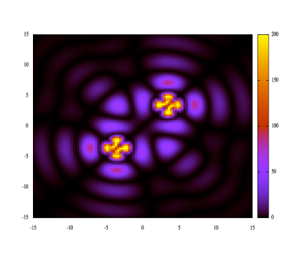
Figure 1: Spectral density of the YSR state with bonding struture of a dimer with parallel classical magnetic moments. The orbital channel is $d_{x^{2}-y^{2}}$.

The quantum phase transition of the classical magnetic impurity bears a resemblance to the Kondo effect of quantum magnetic impurities in superconducting hosts. For impurities with spin $S=1/2$, a Kondo temperature $T_{K}$ is defined such that for $k_{B}T_{K}\ll\Delta$ the impurity behaves as a free spin embedded in a superconductor, while for $k_{B}T_{K}\gg\Delta$ the impurity forms a singlet with bound quasiparticle states. In the former case, singlet combinations of the impurity with quasiparticle states form subgap excitations. In the latter case, there are also subgap excitations, resulting from the broken Kondo singlet. These features are observed in calculations with numerical renormalization group of the Anderson impurity model in a superconducting substrate, zitko1 ; zitko2 as well as experimentally in quantum dots, which behave like magnetic impurities. deacon ; agua

Nadj-Perge and coworkers proposed the construction of artificial structures of magnetic adatoms to realize topological superconductivity, nadj1 which motivated a pletora of recent studies. nadj2 ; pletorap1 ; pletora1 ; pletora2 ; PGvO ; nico ; alf1 ; felix Magnetic adatoms usually have $d$ or $f$ external orbitals. Hence, the impurity may have a more complex structure than a classical magnetic moment coupled to the superconducting substrate. In Ref. moca, the Shiba spectrum of a Mn impurity with 3d active electrons in a two-band superconductor was studied taking into account the atomic orbital degrees of freedom, in addition to the spin. More recently, features related to the orbital structure have been observed with scanning tunneling microscope (STM) experiments. yang ; dj In these systems, the net magnetic moment of the adatoms is originated in a dominant internal Hund rule, while the coupling of the orbital degrees of freedom define multiple channels in the Kondo problem. In normal metal (non-superconducting) substrates, these effects have been studied in the context of the two-orbital Anderson impurity model, corresponding to $S=1$ quantum impurities theoretically, mk1 ; mk2 ; mk3 as well as experimentally.mk4 ; mk5 The additional ingredient that the multi-orbital structure brings about is the possibility of underscreening, in addition to the full screening mechanism taking place in the single-orbital case.

The search for topological phases in structures of YSR states demands the construction of complex arrays containing several adatoms. The simplest of these arrays is a dimer containing two adatoms. Results for a dimer of classical impurities in a s-wave superconductor have been presented in Refs. flatte, ; meng1, ; meng2, and the phase diagram of a dimer of quantum ${\bf S}=1/2$ impurities was studied in Ref. dimer, , while trimers of ${\bf S}=1/2$ impurities have been studied in normal metal artri and superconductingkoerber substrates. All these works focus on adatoms with a single active orbital. The YSR states localized at the impurities in clusters of multiorbital adatoms hybridize through the substrate and many scenarios and phase transitions may take place. In a recent work the transport properties of two impurities realized in a double quantum-dot structure embbeded in a superconducting Josephson junction were analized. alf Experimental research with STM spectroscopy on dimers of Cr and Mn atoms on superconducting substrates has been recently reported in Refs. nacho, ; katha, . Even more recently, dimers and trimers of Gd atoms in superconductors have been also studied with STM techniques in Ref. ding, . Maps like the one shown in Fig. 1 are recorded in these experiments, which reveal details on the multiorbital structure of the adatoms and the hybridization between the impurities mediated by the substrate.

The aim of this work is to present a systematic theoretical framework to analyze the different scenarios expected to take place when clusters of adatoms with several active orbitals are placed in superconducting substrates, considering the net spin of the atoms as classical magnetic moments. We base this description on the definition of an effective Green’s function to describe the bound subgap states, which can be exactly evaluated. In addition, we derive an effective Hamiltonian to calculate the subgap excitations for the case where the impurities are sufficiently diluted. In both cases, not only the spectrum but also the density of states of the YSR states can be calculated and analyzed, taking into account the relative orientation of the magnetic moments, as well as the multiorbital structure of the adatoms and the effect of the crystal field generated by the environment. We illustrate the formalism mainly focusing on dimers with d orbitals and a substrate with a constant density of states, but we also revisit the single multiorbital impurity and a trimer configuration. The general formalism applies to any type of orbitals and can be extended to describe other type of substrates.

The paper is organized as follows. In section II we present details of the derivation of the model describing the hybridization of the multiple orbitals of the impurity with the substrate and we briefly review the derivation of the low energy Hamiltonian for the impurity originally presented in Ref. blandin, . We also discuss with intuitive arguments how the picture of the quantum phase transition taking place as a function of $J$ generalizes when the impurity has several active orbitals and when instead of a single impurity, there are two impurities forming a dimer. This model can be exactly solved with the methods presented in sections III, where we present the derivation of an effective Hamiltonian for the case of diluted impurities. Results are presented in section IV and section V is devoted to summary and conclusions. The appendices contain some technical details.

II Theoretical description

II.1 Model

Typically, magnetic adatoms have up to $2l+1$ active orbitals of angular momentum $l$ that hybridize with the substrate, and a strong intra-atomic Hund rule generating a magnetic moment with total spin $S=(2l+1)/2$. The low-energy model for such an impurity in metallic substrates was originally derived in a seminal paper by Noziéres and Blandin, blandin who considered the most general Anderson impurity model in real metals. Taking into account the orbital structure of the electrons of the impurity that hybridize to the substrate, and the crystal field splitting, they derived the low-energy Hamiltonian where the impurity is represented by a quantum spin in a conducting environment. The latter defines the model to investigate the Kondo effect in realistic scenarios. In what follows, we adapt such derivation to the case of a superconducting substrate. In a second step, we treat the net spin of the impurity as a classical magnetic moment. For simplicity, we will mainly focus on a BCS model for the superconducting host expressed in a basis of plane waves, assuming a pairing interaction with s-wave symmetry. The same steps of our reasoning can be adapted to the case of a substrate of Bloch electrons and to other symmetries of the superconducting order parameter.

It is instructive to derive the Hamiltonian for the multiorbital impurity in the superconducting host following the steps of Ref. tsvelic, . The starting point is the definition of a convenient basis to adequately represent the delocalized degrees of freedom of the substrate and the localized ones at the impurity. The natural basis for the substrate is that of plane waves. In 3D, plane waves can be expanded in spherical waves as follows,

$$\psi_{l,m}({\bf k},{\bf r})=\frac{4\pi(i)^{l}}{\sqrt{\cal V}}j_{l}(kr)Y^{m}_{l}(\hat{n}_{k})Y_{l}^{m}(\hat{n}_{r}),$$ (1)

where ${\cal V}$ is the volume of the system and $j_{l}(kr)$ is the spherical Bessel function of order $l$. On the other hand, for the impurity it is natural to consider a basis constructed with atomic wave functions with well defined angular momentum $l$, $\phi^{imp}_{l,m}({\bf r})=Y_{l,m}(\hat{n}_{r})\phi(r)$, being $Y_{l,m}(\hat{n}_{r})$ the spherical harmonics with $m=-l,\ldots,l$.

The field operator for an electron with spin $\sigma$ can be expanded as follows,

$$\Psi_{\sigma}({\bf r})={\sum_{{\bf k},l,m}}^{\prime}\psi_{l,m}({\bf k},{\bf r}){\bf c}_{\bf k,\sigma}+\sum_{l,m}\phi^{imp}_{l,m}({\bf r}){\bf d}_{l,m,\sigma}.$$ (2)

The $\sum^{\prime}_{\bf k}$ denotes summation over ${\bf k}$-vectors with $k<r_{B}^{-1}$, being $r_{B}$ the Bohr radius, which prevents problems related to the fact that the two basis used in the expansion above are not orthogonal. tsvelic

The Hamiltonian for the impurity in the superconducting host expressed in terms of these field operators reads

$$H = \int d^{3}r\left\{\sum_{\sigma}\Psi_{\sigma}^{\dagger}({\bf r})\left[{\cal H}^{0}_{\sigma,{\rm sup}}+{\cal H}^{0}_{\sigma,{\rm imp}}\right]\Psi_{\sigma}({\bf r})\right.$$ (3)

$$\left.\;\;\;\;\;\;+\Delta\Psi_{\uparrow}^{\dagger}({\bf r})\Psi_{\downarrow}^{\dagger}({\bf r})+H.c.\right\}+H^{\rm Coul}_{\rm imp},$$

where $H^{0}_{\rm sup}$ corresponds to the kinetic term of the Hamiltonian for the superconducting substrate and $H^{0}_{imp}$ is the non-interacting Hamiltonian of the impurity, the first term of the second line is the local usual s-wave BCS-pairing Hamiltonian and $H^{\rm Coul}_{\rm imp}$ is the Coulomb interaction for the electrons in the impurity.

Substituting the expansion of Eq. (2) in the latter Hamiltonian we get an expression in terms of the creation and annihilation operators, which reads

$$H = \sum_{{\bf k}}\left[\sum_{\sigma}\xi_{\bf k}c^{\dagger}_{{\bf k},\sigma}c_{{\bf k},\sigma}+\Delta c^{\dagger}_{{\bf k},\uparrow}c^{\dagger}_{-{\bf k},\downarrow}+H.c.\right]+H_{\rm hyb}$$ (4)

$$+H_{\rm imp}\left[d^{\dagger}_{l,m,\sigma},d_{l,m,\sigma}\right].$$

Here $H_{\rm imp}$ collects all the terms depending on the operators $d^{\dagger}_{l,m,\sigma},\;d_{l,m,\sigma}$ describing the orbital and spin degrees of freedom of the impurity. The term $H_{\rm hyb}$ describes the hybridization terms between the degrees of freedom of the substrate and the ones in the impurity. The corresponding matrix elements are obtained by computing

$$\int drr^{2}d\Omega_{r}\;\psi^{*}_{l^{\prime},m^{\prime}}({\bf k},{\bf r})\left[{\cal H}^{0}_{\rm sup}+{\cal H}^{0}_{\rm imp}\right]\phi^{imp}_{l,m}({\bf r})$$

$$\simeq W_{k,l,m}Y^{m}_{l}(\hat{n}_{k})\delta_{l,l^{\prime}}\delta_{m,m^{\prime}}.$$ (5)

We have used the normalization of the spherical harmonics and we have introduced the parameter

$$W_{k,l,m}=\frac{4\pi(i)^{l}}{\sqrt{\cal V}}\int drr^{2}j_{l}(kr)\left[{\cal H}^{0}_{\rm sup}+{\cal H}^{0}_{\rm imp}\right]\phi_{l,m}(r),$$ (6)

which defines the hybridization amplitude between the atomic orbital with angular momentum $l$ and the substrate. Thus, the hybridization Hamiltonian reads

$$H_{\rm hyb}=\sum_{{\bf k},l,m,\sigma}W_{k,l,m}Y^{m}_{l}(\hat{n}_{k})c^{\dagger}_{{\bf k},\sigma}d_{l,m,\sigma}+H.c.$$ (7)

The latter expression is the starting point of Ref. blandin, , where it is argued that that the hybridization parameter is approximately the same for all $k$, i.e., $W_{k,l,m}\sim W_{l,m}$.

When the impurity is embedded in a lattice, rotational symmetry is broken. Hence, the degenerate levels $m$, are split by the electric potential of the neighboring atoms and $m$ is no longer a good quantum number. This is, precisely, the effect of the crystal field splitting. In this context, the internal atomic levels are more appropriately described by a label which depends on the irreducible representation of the point group of symmetry at the impurity. We will focus on the case of impurities with $d$ electrons ($l=2$), in which case, it is usual to introduce the labeling of the cubic harmonics, $\mu=d_{x^{2}-y^{2}},d_{z^{2}},d_{xy},d_{xz},d_{yz}$, instead of $m$. In a system with crystal field splitting, the hybridization parameter is not expected to be the same for all the atomic channels and it depends on the representation label characterizing the different channels, $W_{\mu}$. Hereafter, we assume that the crystal field is relevant, hence we label with the index $\mu$.

Following again Ref. blandin, , it is possible to eliminate the high-energy states of the impurity by recourse to a Schrieffer-Wolff transformation. Such a procedure consists in integrating out the (high-energy) states associated to the charge fluctuations in the impurity. In the case where all the relevant orbitals labeled by $\mu$ are filled, half-filled or empty, this leads to a Kondo Hamiltonian, where the many-body states of the impurity are projected only on those describing its total spin. If there is a strong Hund rule in the impurity, its total spin is large and it is usual to simplify the low-energy Hamiltonian by representing the spin impurity ${\bf S}$ by a classical magnetic moment. Typically Mn⁺², V⁺² or Ni⁺² in cubic symmetry satisfy these conditions. All these considerations lead to the low-energy Hamiltonian $H_{\rm low}=H_{\rm sup}+H_{\rm int}$ which replaces $H$ of Eq. (4). At this point it is also convenient to introduce Nambu notation for the fermionic operators of the substrate ${\bf c}_{\bf k}=\left(c_{\bf k,\uparrow},c_{\bf k,\downarrow},c^{\dagger}_{-{\bf k},\downarrow},-c^{\dagger}_{-{\bf k},\uparrow}\right)^{T}$. The different terms of $H_{\rm low}$ read

$$H_{\rm sup} = \sum_{\bf k}{\bf c}^{\dagger}_{\bf k}\left[\xi_{\bf k}\tau_{z}+\Delta\tau_{x}\right]\;{\bf c}_{\bf k},$$

$$H_{\rm int} = \sum_{{\bf k},{\bf k}^{\prime}}{\bf c}^{\dagger}_{\bf k}\;V({\bf k},{\bf k}^{\prime})\;{\bf c}_{{\bf k}^{\prime}}.$$ (8)

with

$$V({\bf k},{\bf k}^{\prime}) = \sum_{\mu}f^{*}_{\mu}({\bf k})V_{\mu}f_{\mu}({\bf k}^{\prime})$$

$$V_{\mu} = \left[\;U_{\mu}\tau_{z}+J_{\mu}\;\;\bm{\sigma}\cdot{\bf S}\;\right].$$ (9)

Here $\tau_{x,y,z}$ are Pauli matrices acting in he particle-hole degrees of freedom of the Nambu spinor, while $\bm{\sigma}=\left(\sigma_{x},\sigma_{y},\sigma_{z}\right)$ are Pauli matrices acting on the spin degrees of freedom. The first term of $H_{\rm int}$ is the potential scattering and the second one is the exchange interaction between the total spin of the impurity, ${\bf S}$ (described by a classical vector), and the spin of the electrons in the substrate. The parameters entering the interaction depend on the nature of the substrate and the energy for the impurity charge fluctuations $\Delta E$ as follows

$$J_{\mu},U_{\mu}=\frac{W_{\mu}^{2}}{\Delta E}.$$ (10)

The coefficients $f_{\mu}$ in Eq. (II.1) are in general combinations of the spherical harmonic functions. For the case of $d$ orbitals and a plane-wave substrate, they are the cubic harmonics

$$f_{z^{2}}=Y_{2}^{0},\;\;\;f_{x^{2}-y^{2}}=\frac{1}{\sqrt{2}}\left(Y_{2}^{-2}+Y_{2}^{2}\right),\;\;\;f_{xy}=-\frac{i}{\sqrt{2}}\left(Y_{2}^{-2}-Y_{2}^{2}\right),$$

$$f_{xz}=\frac{1}{\sqrt{2}}\left(Y_{2}^{-1}-Y_{2}^{1}\right),\;\;\;f_{yz}=-\frac{i}{\sqrt{2}}\left(Y_{2}^{-1}+Y_{2}^{1}\right).$$ (11)

We now extend the previous reasoning to the case of $N_{I}$ impurities at positions ${\bf r}_{j},\;j=1,\ldots,N_{I}$, which we assume to be sufficiently separated so that we can neglect any direct hybridization between them. The basis – equivalent to Eq. (2) – to express the Hamiltonian in terms of creation and annihilation operators is now

$$\Psi_{\sigma}({\bf r})=\sum^{\prime}_{{\bf k},\sigma}\psi_{\mu}({\bf k},{\bf r})c_{{\bf k},\sigma}+\sum_{j=1}^{N_{I}}\sum_{l,m}\phi^{\rm imp}_{j,l,m}({\bf r})d_{j,l,m,\sigma},$$ (12)

The basis of functions localized at the impurities are $\phi^{\rm imp}_{j,l,m}({\bf r})=Y_{l,m}(\hat{n}_{{\bf r}-{\bf r}_{j}})\;\phi(|{\bf r}-{\bf r}_{j}|)$, where $\hat{n}_{{\bf r}-{\bf r}_{j}}$ are the angular coordinates of the vector ${\bf r}-{\bf r}_{j}$ and $Y_{l,m}(\hat{\mu}_{{\bf r}-{\bf r}_{j}})$ is a spherical harmonic. For a system with a strong crystal field splitting, it is a combination of spherical harmonics corresponding to the relevant irreducible representation of the point symmetry group. $\phi(|{\bf r}-{\bf r}_{j}|)$ is a function strongly localized at the impurity.

After following the same steps as before, we derive the low-energy Hamiltonian analogous to Eq. (II.1). The corresponding interaction matrix reads

$$V({\bf k},{\bf k}^{\prime}) = \sum_{j=1}^{N_{I}}\sum_{\mu}{f^{j}_{\mu}}({\bf k})^{*}V^{j}_{\mu}f^{j}_{\mu}({\bf k}^{\prime})$$

$$V^{j}_{\mu} = \left[\;U^{j}_{\mu}\tau_{z}+J^{j}_{\mu}\;\;\bm{\sigma}\cdot{\bf S}_{j}\;\right].$$ (13)

being ${\bf S}_{j}$ the classical vector representing the magnetic moment of the $j$-th impurity while

$$U^{j}_{\mu},J^{j}_{\mu}=W_{j}^{2}/\Delta E,\;\;\;\;\;\;\;\;\;\;\;\;f^{j}_{\mu}({\bf k})\equiv e^{-i{\bf k}\cdot{\bf r}_{j}}Y_{\mu}(\hat{n}_{k}),$$ (14)

with all the parameters having the same meaning as in the case of the simple impurity. Notice that, as before, we have substituted the indices $l,m$ by the representation index $\mu$, assuming the effect of the crystal field splitting.

III Formalism

III.1 Green’s function and T-Matrix

We introduce the Nambu notation for the field operators of the electrons in the substrate, $\Psi({\bf r})=\left(\Psi_{\uparrow}({\bf r}),\Psi_{\downarrow}({\bf r}),\Psi^{\dagger}_{\downarrow}({\bf r}),-\Psi^{\dagger}_{\uparrow}({\bf r})\right)$. The corresponding retarded Green’s function in terms of the T-matrix can be expressed as follows

$$G({\bf r},{\bf r},\omega) = G^{0}(0,\omega)+$$

$$\sum_{\mu,\mu^{\prime}}\sum_{j,j^{\prime}}\gamma_{\mu}({\bf r}-{\bf r}_{j},\omega)^{*}\;T^{j,j^{\prime}}_{\mu,\mu^{\prime}}(\omega)\;\gamma_{\mu^{\prime}}({\bf r}_{j^{\prime}}-{\bf r},\omega),$$

where $G^{0}(0,\omega)$ is the local Green’s function of the substrate without impurities. The matrices $\gamma_{\mu}({\bf r},\omega)$ are

$$\gamma_{\mu}({\bf r},\omega)=\sum_{\bf k}e^{i{\bf k\cdot r}}G^{0}({\bf k},\omega)f_{\mu}({\bf k})^{*},$$ (16)

and the $T$-matrix is determined from the equation

$$T^{j,j^{\prime}}_{\mu,\mu^{\prime}}(\omega)=\delta_{j,j^{\prime}}\delta_{\mu,\mu^{\prime}}V_{\mu}^{j}+\sum_{j^{\prime\prime},\mu^{\prime\prime}}T_{\mu,\mu^{\prime\prime}}^{j,j^{\prime\prime}}(\omega)F_{\mu^{\prime\prime},\mu^{\prime}}^{j^{\prime\prime},j^{\prime}}(\omega)V_{\mu^{\prime}}^{j^{\prime}},$$ (17)

with

$$F_{\mu,\mu^{\prime}}^{j,j^{\prime}}(\omega)=\sum_{\bf k}f^{j}_{\mu}({\bf k})^{*}G^{0}({\bf k},\omega)f^{j^{\prime}}_{\mu^{\prime}}({\bf k}).$$ (18)

The eigenenergies of the Shiba states are determined from the energies of the poles of the $T$-matrix within the gap. It is interesting to notice that the $T$-matrix of Eq. (17) couples different impurities and different channels, in spite of the fact that the bare interaction $V$ is diagonal in these indices. This represents an effective interaction mediated by the substrate that is not present in the original model and plays a key role in the nature of the hybridization of the Shiba states. In the case of a single impurity, due to the orthogonality of the functions $f^{j}_{\mu}({\bf k})$, the function $F$ reduces to

$$F(\omega)=\sum_{\bf k}G^{0}({\bf k},\omega)$$ (19)

while the $T$-matrix is diagonal in the orbital index and reads

$$T_{\mu}(\omega)=V_{\mu}\left[1-F(\omega)V_{\mu}\right]^{-1}.$$ (20)

III.2 Subgap Green’s function and Shiba states

The aim of the present section is to define an effective Green’s function $\hat{\cal G}(\omega)$ to represent the Shiba states. We define it as follows,

$$\hat{T}(\omega)=\hat{V}\;\hat{\cal G}(\omega)\;\hat{V}\;\;\;\;\;\;\;\;\;|\omega|<\Delta,$$ (21)

where we $\hat{T}(\omega)$ and $\hat{V}$ are matrices in the impurity, orbital and Nambu indices. In this way, this Green’s function has poles at the Shiba energies and the corresponding quasiparticle weight defines the contribution of the Shiba states to the local density of states.

III.2.1 Single impurity

We consider the $T$-matrix defined in Eq. (20). The eigenenergies of the Shiba states correspond to the poles of this matrix within the range $|\omega|<\Delta$, and are determined from the condition $\mbox{Det}[1-F_{\mu}(\omega)V_{\mu}]=0$.

We are now interested in constructing an effective Green’s function ${\cal G}_{\mu}(\omega)$, such that its poles in the range of energies with $|\omega|<\Delta$ coincide with those of the $T$-matrix. We define an auxiliary matrix such that its zeroes coincide with the zeroes of ${\cal G}^{-1}_{\mu}(\omega)$, hence with the poles of ${\cal G}_{\mu}(\omega)$,

$$\Lambda_{\mu}(\omega)=V_{\mu}-V_{\mu}F_{\mu}(\omega)V_{\mu}.$$ (22)

In order to find the zeroes of this matrix, it is convenient to diagonalize it for each $\omega$ and express it in terms of the corresponding eigenvalues $\epsilon_{m}$ and eigenstates $|\Phi_{m}\rangle$ as follows,

$$\Lambda_{\mu}(\omega)=\sum_{m}\epsilon_{m}(\omega)|\Phi_{m}(\omega)\rangle\langle\Phi_{m}(\omega)|.$$ (23)

The Shiba state $|{\mu,\rm s}\rangle$ with energy $E_{\mu,\rm s}$ corresponds to the condition that one of these eigenstates has vanishing eigenvalue $\epsilon_{m}(E_{\mu,\rm s})=0$. Due to the Nambu structure, they have opposite energies, $E_{\mu,+}=-E_{\mu,-}$, since the two states are related by a charge-conjugation and time reversal (${\rm CT}$) transformation. The latter reads $|\mu,-\rangle={\rm CT}|\mu,+\rangle$ with ${\rm C}=-i\tau_{y}$ and ${\rm T}=i\sigma_{y}K$, being $K$ is the complex conjugation operation.

Since we are looking for a Green’s function with poles at the energies $E_{\mu,\rm s}$, its inverse must satisfy

$${\cal G}^{-1}_{\mu}(E_{\mu,\rm s})|{\mu,\rm s}\rangle = \left[V_{\mu}-V_{\mu}F_{\mu}(E_{\mu,\rm s})V_{\mu}\right]|{\mu,\rm s}\rangle=0.$$ (24)

In order to get an expression for ${\cal G}^{-1}_{\mu}(\omega)$ in a neighborhood of the Shiba energy, $\omega\simeq E_{\mu,\rm s}$, we perform the following expansion

$$\left[{\cal G}^{-1}_{\mu}(\omega)\right]_{\rm s}\simeq\left[{\cal G}^{-1}_{\mu}(E_{\mu,\rm s})\right]_{\rm s}+Z_{\mu,\rm s}^{-1}(\omega-E_{\mu,\rm s}),$$ (25)

where we have introduced the notation $\left[{\cal G}^{-1}_{\mu}(\omega)\right]_{\rm s}=\langle{\mu,\rm s}|{\cal G}^{-1}_{\mu}(\omega)|{\mu,\rm s}\rangle$, hence, $\left[{\cal G}^{-1}_{\mu}(E_{\mu,\rm s})\right]_{\rm s}=0$ and the quasiparticle weight $Z_{\mu,\rm s}$ such that

$$Z_{\mu,\rm s}^{-1}=\left[\frac{\partial{\cal G}_{\mu}^{-1}(\omega)}{\partial\omega}\right]_{\rm s,E_{\mu,\rm s}}.$$ (26)

In this way, the explicit expression for the subgap Green’s function in the basis of Shiba states reads,

$${\cal G}_{\mu}(\omega)=\sum_{\rm s}\;|{\mu,\rm s}\rangle\frac{Z_{\mu,\rm s}}{\omega-E_{\mu,\rm s}+i\eta}\langle{\mu,\rm s}|,$$ (27)

where we have introduced an infinitesimal $\eta>0$ to regularize the denominator. For a single impurity, we typically have two Shiba states per orbital channel.

With these definitions, we can write the spin-resolved spectral density for the particle and hole components of a given Shiba state with energy $E_{\mu,\rm s}$ as

$$\rho_{\sigma}^{e,h}({\bf r},E_{\mu,\rm s})=\mbox{Tr}\Big{[}\Pi^{e,h}_{\sigma}\gamma_{\mu}({\bf r},E_{\mu,\rm s})\;\rho_{\mu,\rm s}\;\gamma_{\mu}({\bf r},E_{\mu,\rm s})\Big{]},$$ (28)

where $\rho_{\mu,\rm s}=\pi Z_{\mu,\rm s}|\mu,\rm s\rangle\langle\mu,\rm s|$, while $\Pi^{e,h}_{\sigma}$ projects on the subspace of electrons ($e$), holes ($h$) and spin $\sigma$.

In the case of a single impurity embedded in a substrate with a constant density of states $\nu$ we can get some simple expressions for the energies of the Shiba states. Also, for vanishing scattering potential, the structure of the Shiba states simplifies and we can also get simple analytical expressions for the quasiparticle weights.

Using the expression of the matrix $F$, defined in Eq. (19), and calculated in Appendix A for a constant density of states,

$$F(\omega)=-\frac{\pi\nu}{\sqrt{\Delta^{2}-\omega^{2}}}\sigma_{0}\left[\omega\tau_{0}+\Delta\tau_{x}\right],\;\;\;\;|\omega|<\Delta,$$ (29)

we can analytically calculate the energies of the Shiba states from the zeroes of the auxiliary matrix defined in Eq. (22). This leads to

$$\mbox{Det}\left[1-F(\omega)V_{\mu}\right]=\mbox{Det}\left\{\tau_{0}\sigma_{0}+\frac{\pi\nu}{\sqrt{\Delta^{2}-\omega^{2}}}\left[\omega\left(U_{\mu}\tau_{z}\sigma_{0}\right.\right.\right.$$

$$\left.\left.\left.\;\;\;\;\;\;\;\;\;\;\;\;\;+J_{\mu}S\sigma_{z}\tau_{0}\right)+\Delta\left(iU_{\mu}\tau_{y}\sigma_{0}+J_{\mu}S\tau_{x}\sigma_{z}\right)\right]\right\}=0.$$ (30)

After simple algebra, we get the energies for the Shiba subgap states,yang

$$E_{\mu}^{\pm}=\pm\Delta\frac{\left(1+\beta_{\mu}^{2}-\alpha_{\mu}^{2}\right)}{\sqrt{4\alpha_{\mu}^{2}+\left(1-\alpha_{\mu}^{2}+\beta_{\mu}^{2}\right)^{2}}},$$ (31)

being $|\mu,\pm\rangle$ the corresponding states, with

$$\alpha_{\mu}=\frac{J_{\mu}}{J_{0}},\;\;\;\;\;\;\;J_{0}=\frac{1}{\pi\nu S},\;\;\;\;\;\;\;\beta_{\mu}=U_{\mu}\pi\nu.$$ (32)

If we assume $U_{\mu}>0$, the crossing of the two Shiba states, corresponding to $E_{\mu}^{\pm}=0$, takes place when $J_{\mu}$ achieves the critical value

$$J_{\mu}^{c}=J_{0}\sqrt{1+\beta_{\mu}^{2}}.$$ (33)

The corresponding Shiba states $|\mu,\pm\rangle$ have a very simple form in the case of vanishing potential scattering $U_{\mu}=0$. They read

$$|\mu,+\rangle = (0,1,0,-1)^{T},\;\;\;\;\;\;\;\;|\mu,-\rangle=(1,0,1,0)^{T},$$ (34)

for $J<J_{\mu}^{c}$, with $\pm$ corresponding to the labeling of Eq. (31). The roles of $\pm$ are interchanged in Eq. (34) for $J>J_{\mu}^{c}$.

The quasiparticle weights defined in Eq. (26) can be calculated from

$$Z_{\mu,{\rm s}}^{-1} = -\langle\mu,{\rm s}|V_{\mu}\left[\frac{\partial F_{\mu}(\omega)}{\partial\omega}\right]_{E_{\mu,{\rm s}}}V_{\mu}|\mu,{\rm s}\rangle$$

$$= \frac{\nu\pi}{\sqrt{\Delta^{2}-E_{\mu,{\rm s}}^{2}}}\langle\mu,{\rm s}|V_{\mu}\left[\tau_{0}+\frac{\Delta E_{\mu,{\rm s}}}{\Delta^{2}-E_{\mu,{\rm s}}^{2}}\tau_{x}\right]V_{\mu}|\mu,{\rm s}\rangle.$$

This expression significantly simplifies for deep Shiba states which correspond to $|E_{\mu,{\rm s}}|\ll\Delta$,

$$Z_{\mu,{\rm s}}^{-1}\simeq\frac{\nu\pi}{\Delta}\langle\mu,{\rm s}|V^{2}_{\mu}|\mu,{\rm s}\rangle.$$

For vanishing scattering potential, $U_{\mu}\sim 0$, they simplify further and read $Z_{\mu,{\rm s}}^{-1}\simeq\nu\pi(SJ_{\mu})^{2}/\Delta$.

III.2.2 Several impurities

We can easily generalize the procedure explained before to calculate the energies of the Shiba states in the case of many impurities. As before, we start by defining the matrix

$$\hat{\Lambda}(\omega)=\hat{V}-\hat{V}\hat{F}(\omega)\hat{V}$$ (36)

and diagonalize it for every $\omega$. Here, the matrices $\hat{V}$ and $\hat{F}$ enclose all the matrix elements of $V^{j}_{\mu}$ and $F^{j,j^{\prime}}_{\mu,\mu^{\prime}}(\omega)$. We denote the corresponding basis of Nambu spinors as $|j,\mu\rangle$. Then, for each $\omega$, we have an expression identical to Eq. (23), with the Shiba energy defined from the condition that some eigenvalue vanishes. There are $2N_{s}$ of such states, being $N_{s}$ the number of impurities times the number of orbitals. We name the corresponding Shiba energies $E_{\ell,\rm s},\;\ell=1,\ldots,N_{s}$, ${\rm s}=\pm$ and the corresponding eigenvectors are $|\ell,\pm\rangle$, with $E_{\ell,+}=-E_{\ell,-}$ and $|\ell,-\rangle={\rm CT}\;|\ell,+\rangle$.

The generalization of Eq. (27) for the case of many impurities reads

$$\hat{\cal G}_{\ell}(\omega)=\sum_{\rm s=\pm}\;|\ell,{\rm s}\rangle\frac{Z_{\ell,\rm s}}{\omega-E_{\ell,\rm s}+i\eta}\langle\ell,{\rm s}|,$$ (37)

and the spin-resolved spectral density for the particle and hole components of the Shiba states is evaluated in a similar way to the case of a single impurity. For a given state with eigenenergy $E_{\ell,\rm s}$ it reads

$$\rho_{\sigma}^{e,h}({\bf r},E_{\ell,\rm s})=\sum_{\mu,\mu^{\prime}j,j^{\prime}}\mbox{Tr}\left[\Pi^{e,h}_{\sigma}\gamma_{\mu}({\bf r}-{\bf r}_{j},E_{\ell,\rm s})\;\hat{\rho}_{\ell,\rm s}\;\gamma_{\mu^{\prime}}({\bf r}_{j^{\prime}}-{\bf r},E_{\ell,\rm s})\right],$$ (38)

with $\hat{\rho}_{\ell,\rm s}=\pi Z_{\ell,\rm s}|\ell,\rm s\rangle\langle\ell,\rm s|$. Here we recall that the Shiba states $|\ell,\rm s\rangle$ are expanded by the Nambu spinors $|j,\mu\rangle$.

III.3 Effective tight-binding - BCS model for dilute impurities

The matrix elements $F^{j,j^{\prime}}_{\mu,\mu^{\prime}}(\omega)=F^{j^{\prime},j}_{\mu^{\prime},\mu}(\omega)$ define an effective interaction between electrons in subgap states localized at the impurities. The strength of this interaction depends on the separation between the impurities $r_{j,j^{\prime}}$ relative to the coherence length of the superconductor $\xi_{0}$ and to the wavelength $k_{F}^{-1}$. Typically, $r_{j,j^{\prime}}\leq\xi_{0}$. We focus on a situation where the impurities are sufficiently diluted to justify a perturbative treatment of the off-diagonal elements $F^{j,j^{\prime}}_{\mu,\mu^{\prime}}$, with $j\neq j^{\prime}$. This corresponds to distances satisfying $k_{F}r_{j,j^{\prime}}\gg 1$. Under these conditions we can solve the equation for the Shiba states starting from the solution of the isolated impurities and derive an effective Hamiltonian. Our strategy is to get a convenient expression for the inverse of the subgap Green’s function defined in Eq. (36) in this limit and then to identify the effective Hamiltonian $\hat{H}_{\rm eff}$ from the relation

$$\hat{\cal G}^{-1}(\omega)=\left(\omega\hat{1}-\hat{H}_{\rm eff}\right).$$ (39)

where $\hat{1}$ is the identity matrix. We start by writing $\hat{\cal G}^{-1}(\omega)$ for the $N$-impurity case as follows,

$$\hat{\cal G}^{-1}(\omega)=\sum_{j,\mu}\left[{\cal G}^{-1}(\omega)\right]_{\mu}^{j}+\sum_{j,j^{\prime},\mu,\mu^{\prime}}\left[{\cal G}^{-1}(\omega)\right]^{j,j^{\prime}}_{\mu,\mu^{\prime}},$$ (40)

with

$$\left[{\cal G}^{-1}(\omega)\right]_{\mu}^{j} = V_{\mu}^{j}-V_{\mu}^{j}F_{\mu}^{j,j}(\omega)V_{\mu}^{j},$$

$$\left[{\cal G}^{-1}(\omega)\right]^{j,j^{\prime}}_{\mu,\mu^{\prime}} = V_{\mu}^{j}F_{\mu,\mu^{\prime}}^{j,j^{\prime}}(\omega)V_{\mu}^{j^{\prime}},\;\;\;\;\;j\neq j^{\prime}.$$ (41)

For energies close to the Shiba energies for the single impurities, $E_{j,\mu\rm s}$, we expand $\hat{\cal G}^{-1}(\omega)$ with respect to this value. Projecting on the states $|j,\mu,{\rm s}\rangle=1/\sqrt{Z_{j,\mu,\rm s}}|\mu,{\rm s}\rangle^{j}$, where $|\mu,{\rm s}\rangle^{j}$ are the Shiba states of the isolated impurity $j$, and considering the inter-impurity terms as perturbations, we have

$$\left[{\cal G}^{-1}(\omega)\right]_{\mu}^{j} \simeq \sum_{\rm s}|j,{\mu,\rm s}\rangle\left(\omega-E_{j,\mu,\rm s}\right)\langle j,\mu,{\rm s}|,$$ (42)

$$\left[{\cal G}^{-1}(\omega)\right]^{j,j^{\prime}}_{\mu,\mu^{\prime}} \simeq \sum_{{\rm s},{\rm s}^{\prime}}|j,{\mu,\rm s}\rangle\;h_{\mu s,\mu^{\prime}s^{\prime}}^{j,j^{\prime}}(\omega)\;\langle j^{\prime},\mu^{\prime},{\rm s}^{\prime}|,$$

being

$$h_{\mu s,\mu^{\prime}s^{\prime}}^{j,j^{\prime}}(\omega)=\sqrt{Z_{j,\mu,\rm s}Z_{j^{\prime},\mu^{\prime},{\rm s}^{\prime}}}\langle j,\mu,{\rm s}|V_{\mu}^{j}F_{\mu,\mu^{\prime}}^{j,j^{\prime}}(\omega)V_{\mu^{\prime}}^{j^{\prime}}|j^{\prime},\mu^{\prime},{\rm s}^{\prime}\rangle.$$ (43)

If we assume that the Shiba states are deep in energy, $E_{\mu,\rm s}\sim 0$, we can approximate $h_{\mu s,\mu^{\prime}s^{\prime}}^{j,j^{\prime}}(\omega)\sim h_{\mu s,\mu^{\prime}s^{\prime}}^{j,j^{\prime}}(0)$. We have verified in the explicit calculations that this approximation also works for high-energy Shiba states with $E_{\mu,\rm s}\sim\Delta$, since this function depends mildly on $\omega$ for sufficiently distant impurities.

Thus, the effective Hamiltonian in the basis of Shiba states of the isolated impurities reads

$$\left[\hat{H}_{\rm eff}\right]_{j,j} = \sum_{\mu,s}|j,{\mu,s}\rangle\;E_{j,\mu,s}\;\langle j,\mu,s|,$$ (44)

$$\left[\hat{H}_{\rm eff}\right]_{j,j^{\prime}} = \sum_{s,s^{\prime},\mu,\mu^{\prime}}|j,\mu,{\rm s}\rangle\;h_{\mu s,\mu^{\prime}s^{\prime}}^{j,j^{\prime}}(0)\;\langle j^{\prime},\mu^{\prime},{\rm s}^{\prime}|,\;\;j\neq j^{\prime},$$

where the effective inter-impurity interaction is given by the second line of Eq. (44).

In order to get analytical expressions for the matrix elements, we introduce some simplifying assumptions. In particular, we focus on the case where the scattering potentials $U_{\mu}$ can be neglected, in which case, the Shiba states can be simply expressed as in Eq. (34). Notice, however, that the latter are expressed in the quantization axis for the spin oriented along the magnetic moment of the impurity. In general, the impurities have different orientations $\hat{\bf S}_{j}={\bf S}_{j}/S=\left(\sin\theta_{j}\cos\phi_{j},\sin\theta_{j}\sin\phi_{j},\cos\theta_{j}\right)$. Hence, the Shiba states localized at the impurity $j$ read

$$|j,\mu,+\rangle = \left(|j+\rangle,|\overline{j+}\rangle\right)^{T},$$

$$|j,\mu,-\rangle = \left(|j-\rangle,|\overline{j-}\rangle\right)^{T},$$ (45)

with $|\overline{j\pm}\rangle={\rm T}|j\pm\rangle$ and

$$|j-\rangle = \left(\cos(\theta_{j}/2),\;\sin(\theta_{j}/2)e^{i\phi_{j}}\right)^{T},$$

$$|j+\rangle = \left(-\sin(\theta_{j}/2)e^{-i\phi_{j}},\;\cos(\theta_{j}/2)\right)^{T}.$$ (46)

This leads to the following structure for the effective Hamiltonian

$${\cal H}_{\rm eff}=\left(\begin{array}[]{cc}{\cal H}_{\mu,\mu^{\prime}}^{jj^{\prime}}&\Delta_{\mu,\mu^{\prime}}^{jj^{\prime}}\\ (\Delta_{\mu,\mu^{\prime}}^{jj^{\prime}})^{\dagger}&-({\cal H}_{\mu,\mu^{\prime}}^{jj^{\prime}})^{*}\end{array}\right).$$ (47)

The diagonal matrix elements are $h^{jj}_{\mu,\mu}=E^{j}_{\mu,+}$, while the other matrix elements have the form

$${\cal H}_{\mu,\mu^{\prime}}^{jj^{\prime}}=\eta_{\mu,\mu^{\prime}}^{jj^{\prime}}\langle j+|j^{\prime}+\rangle,\;\;\;\;\;\;\;\;\;\;\Delta_{\mu,\mu^{\prime}}^{jj^{\prime}}=\delta_{\mu,\mu^{\prime}}^{jj^{\prime}}\langle j+|j^{\prime}-\rangle,\;\;\;j\neq j^{\prime}.$$ (48)

Explicit expressions for the $\eta_{\mu,\mu^{\prime}}^{jj^{\prime}}$ and $\delta_{\mu,\mu^{\prime}}^{jj^{\prime}}$ for the case of a substrate modeled by plane waves will be presented in the next Section.

The spectrum of Shiba states in this regime is given by the eigenenergies of ${\hat{H}}_{\rm eff}$, which we name them $\tilde{E}_{\ell,\rm s}$ and $|\ell,\rm s\rangle_{\rm eff}$ are the corresponding eigenstates. These states can be used to calculate the spectral density in the dilute regime. The corresponding expression reads

$$\rho_{\rm eff,\sigma}^{e,h}({\bf r},\tilde{E}_{\ell,\rm s})=\sum_{\mu,\mu^{\prime}j,j^{\prime}}\mbox{Tr}\left[\Pi^{e,h}_{\sigma}\gamma_{\mu}({\bf r}-{\bf r}_{j},\tilde{E}_{\ell,\rm s})\;\hat{\rho}^{\rm eff}_{\ell,\rm s}\gamma_{\mu^{\prime}}({\bf r}_{j^{\prime}}-{\bf r},\tilde{E}_{\ell,\rm s})\right],$$ (49)

where $\hat{\rho}^{\rm eff}_{\ell,\rm s}$ is the density operator associated to the eigenstates of the effective Hamiltonian expanded in the basis of the Nambu spinors $|j,\mu\rangle$.

IV Results

IV.1 Heuristic description of the YSR states in single impurities and dimers

As an introduction to the formal analysis based on the numerical solution of the subgap Green’s function and the effective Hamiltonian presented before, we find it convenient to start by providing some qualitative arguments. We review the quantum phase transition in a single-orbital classical impurity and infer on the basis of simple arguments, how this picture generalizes in the mutiorbital case. We also extend our analysis to the case of a dimer.

Fig. 2 shows sketches of the expected scenarios for a single-orbital impurity. Assuming antiferromagnetic coupling between the impurity and the superconductor, for $J<J^{c}$ the electronic ground state is formed of Cooper pairs, $|\psi_{0}\rangle=|BCS\rangle$ and the subgap excitation with positive energy corresponds to creating a quasiparticle with spin antiparallel to the impurity on the ground state $|\psi_{1}\rangle=\gamma^{\dagger}_{\downarrow}|\psi_{0}\rangle$. Instead, for $J>J^{c}$, the quasiparticle gets bound to the impurity and the roles of the states $|\psi_{0}\rangle$ and $|\psi_{1}\rangle$ are interchanged, $|\psi_{1}\rangle$ becoming the ground state. The excited state corresponds to annihilating the bound quasiparticle. Each of these states have weights on particle and hole states of the free-electron basis. For a finite scattering potential interaction $U>0$, these weights are different.

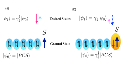
Figure 2: Sketch of the expected scenarios for the ground state and excited states with positive energy of a single-orbital impurity with spin $S$ antiferromagnetically coupled to a BCS substrate. (a) $J<J^{c}$. The ground state is a free impurity in the BCS condensate of the substrate. Subgap excited states correspond to quasiparticles with electron and hole components with the electron component oriented antiparallel to the impurity. (b) $J>J^{c}$. The ground state changes parity and consists of a BCS condensate plus a quasiparticle bounded to the impurity. The excited state corresponds to annihilating the bounded quasiparticle of the ground state. Particle and hole components of the excitations are, respectively, represented by solid and dashed arrows. The dominant component for positive scattering potential is represented in dark color and larger size of the arrow.

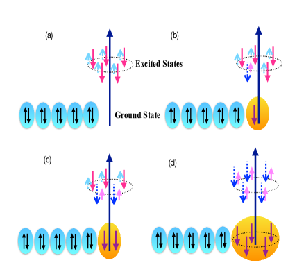
Figure 3: Sketch of the expected scenarios for the ground state and excited states with positive energy of an impurity with several orbitals placed in a superconducting substrate with crystal-field splitting. Particle and hole components of the excitations are, respectively, represented by solid and dashed arrows. The dominant component is represented in dark color and larger size of the arrow. (a) $J_{\mu}<J_{\mu}^{c},\;\forall\mu$. The impurity is completely unscreened. The ground state consists of a BCS condensate and a free magnetic moment. (b) One of the channels is strongly coupled with $J_{\nu}>J_{\mu}^{c}$ while the others have $J_{\mu}<J_{\mu}^{c},\;\mu\neq\nu$. The ground state is a BCS condensate plus a quasiparticle bounded to the impurity. (c) Two channels are strongly coupled and the others are weakly coupled. (d) Quasiparticles in all the available channels are bounded to the impurity. The ground state has total spin zero and the impurity is completely screened.

For a multiorbital impurity with weak $J_{\mu}$ compared to $\Delta$, the ground state corresponds to the free impurity in the BCS condensate of the substrate, while the YSR states correspond to quasiparticle subgap excitations with electron component antiparallel to the impurity in all the orbital channels. This situation is illustrated in Fig. 3 (a). In the opposite limit, when the exchange couplings overcome a critical value $J_{\mu}^{c}$ given by Eq. (33), quasiparticles in all the channels get bound to the impurity and the ground state corresponds to the BCS condensate of the substrate plus the $2l+1$ bound quasiparticles antiparallel to the impurity. This is illustrated in Fig. 3 (d) and it is akin to the quantum phase transition of the single orbital case. The difference consists in the fact that the change of parity in the ground states takes place in the different orbital channels. Making an analogy to the Kondo problem for quantum impurities, the picture of Fig. 3 (a) corresponds to the unscreened impurity, while that of Fig. 3 (d) corresponds to the fully screened impurity. The regime analogous to the underscreened Kondo effect of the quantum impurity corresponds to a ground state having bound quasiparticles only in some of the orbital channels, as illustrated in Figs. 3 (b) and (c).

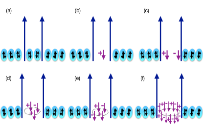
Figure 4: Sketch of the expected scenarios for the ground state of two impurities with several orbitals placed in a superconducting substrate with crystal-field splitting with the net spin aligned in the same direction and separated by a distance $r>k_{F}^{-1}$. The YSR states form in bonding $(+)$ and antibonding $(-)$ combinations of states localized at the impurities. (a) The impurities are completely unscreened. The ground state has total spin $2S$. (b) The bonding combination of one of the angular-momentum channels is bounded, while the others become unbounded. (c) (d) (e) The impurities are partially screened by bonding and/or antibonding states in different channels. (f) Bonding and antibonding states in all the channels are bounded and the impurity is fully screened.

For dimers, the scenario depends crucially on the relative alignment of the magnetic moments. Intuitively, we can expect to easily generalize the scenario of a single impurity in the case of two with parallel magnetic moments. Here it is also important to take into account the inter-impurity distance $r$, relative to the localization length of the YSR of the single impurity. As mentioned before, there are two relevant length scales in the problem, which set the localization length of the YSR states of the single impurity. One is the Fermi wave length $\lambda_{F}=2\pi/k_{F}$, and the other is the superconducting coherence length $\xi_{0}$ for the electrons in the substrate. The usual case in experiments is $\xi_{0}\gg\lambda_{F}$. PGvO For $r\ll\lambda_{F}$, the dimer behaves as an effective impurity with magnetic moment $2S$, while in the limit $r\gg\lambda_{F}$ its behaves as two independent single impurities. For intermediate distances, the YSR states associated to the single impurity hybridize forming bonding $(+)$ and antibonding $(-)$ combinations in every orbital channel. Furthermore, depending on the symmetry of the substrate and of the orbitals, it is also posible that two or more orbital channels hybridize. Depending on the strength of the exchange interaction, none, some, or all of these combined states may cross zero energy, leading to several quantum phase transitions, in which the impurities can be unscreened, underscreened or fully screened. This bears resemblance to the scenario of the single impurity as illustrated in Fig. 4.

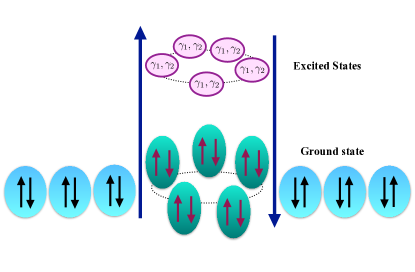
Figure 5: Sketch of the ground state and excited states of two impurities with several orbitals placed in a superconducting substrate with crystal-field splitting with the magnetic moments aligned in opposite directions and separated by a distance $r>\lambda_{F}$. The YSR states are paired and the excitations, represented with $\gamma_{1},\gamma_{2}$ in every channel, are degenerate.

For dimers of identical impurities with magnetic moments aligned in opposite directions the scenario is very different. For $r>\lambda_{F}$, the YSR states of the individual impurities are coupled only through a pairing interaction. Depending on the symmetry this can be intra-channel or inter-cannel. The ground state is the BCS condensate of the substrate plus the BCS ground state of the paired YSR states. The subgap excitations are the Bogoliubov excitations of the latter BCS state. This is illustrated in Fig. 5.

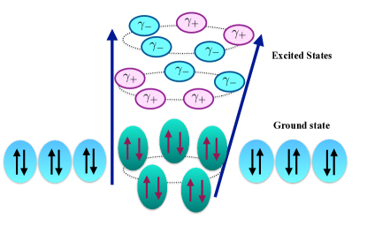
Figure 6: Sketch of the ground state and excited states of two impurities with several orbitals placed in a superconducting substrate with crystal-field splitting with the magnetic moments aligned forming an angle $\theta\neq 0,\pi$ in opposite directions and separated by a distance $r>\lambda_{F}$. The excitations disperse in symmetric and antisymmetric combinations represented by $\gamma_{+},\gamma_{-}$.

The intermediate situation, where the magnetic moments of the impurities are oriented forming a relative angle $\theta\neq 0,\pi$, is illustrated in Fig. 6. In this case there is a combination of a normal hybridization and pairing of the YSR states of the individual impurities. The ground state is similar to that of the antiparallel states and consists of a BCS condensate of the substrate plus the BCS state of the pairs of YSR of the individual impurities. The excited states are Bogoliubov excitations of the latter BCS state but in the present case, they disperse as a consequence of the normal hybridization, forming symmetric and antisymmetric combinations. In the present configuration of the magnetic moments, time-reversal symmetry is broken. Eventually, some of these quasiparticle excitations may cross zero energy, changing the parity of the ground state. This feature is similar to the case of parallel impurities, although the nature of the quasiparticles is different in the two cases. This is the scenario favoring the topological phase in long chains of adatoms. nadj1 ; nadj2 ; PGvO

IV.2 Numerical results

We present results for the case a substrate modeled by plane waves with crystal field splitting, focusing on impurities with atomic orbitals $d_{z^{2}},d_{x^{2}-y^{2}},d_{xy},d_{xz},d_{yz}$ and spin $S=5/2$. We will focus on the case of vanishing potential scattering and assuming the same strength of the exchange interaction for all the impurities, $V_{\mu}^{j}=J_{\mu}\;\bm{\sigma}\cdot{\bf S}_{j}$, with ${\bf S}_{j}=S(\sin\theta_{j}\cos\phi_{j},\;\sin\theta_{j}\sin\phi_{j},\;\cos\theta_{j})$. We also consider that impurities separated by a distance $r$.

The evaluation of the matrix elements of $F$ defined in Eq. (18) in a plane-wave substrate with a constant density of states is presented in Appendix A for energies within the gap, $|\omega|\leq\Delta$. The results depend strongly on the nature of the substrate and the different cases can be summarized as follows

$$F^{j,j}(\omega) = -\frac{\nu\pi}{\sqrt{\Delta^{2}-\omega^{2}}}\sigma_{0}\left[\omega\tau_{0}+\Delta\tau_{x}\right],$$

$$F^{j\neq j^{\prime}}_{\mu,\mu^{\prime}}(\omega) = -4\pi\nu\sum_{l}(i)^{l}\;{\cal C}_{\mu,\mu^{\prime}}(l)\left[\left(\omega\tau_{0}+\Delta\tau_{x}\right)I^{(l)}_{1}(r_{j,j^{\prime}},\omega)\right.$$

$$\left.+\tau_{z}I^{(l)}_{2}(r_{j,j^{\prime}},\omega)\right].$$

The coefficients ${\cal C}_{\mu,\mu^{\prime}}(l)$ are combinations of spherical harmonics and are specified in Eq. (A.2). The functions $I^{(l)}_{1,2}(r)$, defined in Eq. (63) involve integrals of spherical Bessel functions and integer Bessel functions, which are evaluated in Appendix C. Besides exponentially decaying factors $\propto\exp\left(-\sqrt{1-(\omega/\Delta)^{2}}\;r/\xi_{0}\right)$, being $\xi_{0}=v_{F}/\Delta$, these functions also decay with the distance as powers of $1/(k_{F}r)$.

The scattering potential does not play a crucial role in introducing different energy scales for the different channels in the case of clusters. This is because the interesting physics of clusters is dominated by the effective interaction between impurities, mediated by the substrate. The latter behaves differently in the different channels $\mu$. This is determined by the inter-impurity matrix elements given in Eq. (IV.2). In general, they have inter-channel components, in addition to the intra-channel ones. In practice, several of these inter-channel components vanish because of symmetry reasons. With Eqs. (IV.2) we can calculate the exact spectrum of YSR states following Section III.

In order to calculate the effective Hamiltonian in the dilute limit, where the distance $r\gg\lambda_{F}$, we need the function $h_{\mu,\mu^{\prime}}$ defined in Eq. (43). From the calculations presented in Appendix A we get

$$h_{\mu s,\mu^{\prime}s^{\prime}}^{j,j^{\prime}}(0)=-\frac{4\pi\Delta}{(JS)^{2}}e^{-r/\xi_{0}}\sum_{l}(i)^{l}\;{\cal C}_{\mu,\mu^{\prime}}(l)$$ (51)

$$\;\;\;\;\;\;\times\langle j,\mu^{\prime},{\rm s}|V_{\mu^{\prime}}^{j}\left[\tau_{x}\kappa^{(l)}_{1}(k_{F}r)+\tau_{z}\kappa^{(l)}_{2}(k_{F}r)\right]V_{\mu^{\prime}}^{j^{\prime}}|j^{\prime},\mu^{\prime},{\rm s}^{\prime}\rangle.$$

The functions $\kappa^{(l)}_{1,2}(k_{F}r)$ are defined in Eqs. (74), (C.0.2) and (C.0.3).

The coefficients $\eta_{\mu,\mu^{\prime}}^{jj^{\prime}}$ and $\delta_{\mu}^{jj^{\prime}}$ introduced in Eqs. (48), can be calculated Eqs. (43) and (51), using Eq. (III.3). The result is

$$\eta_{\mu,\mu^{\prime}}^{jj^{\prime}} = -4\pi\Delta e^{-r/\xi_{0}}\sum_{l}(i)^{l}\;{\cal C}_{\mu,\mu^{\prime}}(l)\kappa^{(l)}_{1}(k_{F}r),$$

$$\delta_{\mu,\mu^{\prime}}^{jj^{\prime}} = 4\pi\Delta e^{-r/\xi_{0}}\sum_{l}(i)^{l}\;{\cal C}_{\mu,\mu^{\prime}}(l)\kappa^{(l)}_{2}(k_{F}r).$$ (52)

Following Ref. PGvO, we can explicitly calculate the scalar products and perform a gauge transformation to eliminate irrelevant phases. The result is

$$\langle j+|j^{\prime}+\rangle = \cos\frac{\theta_{j}}{2}\cos\frac{\theta_{j^{\prime}}}{2}e^{i(\frac{\phi_{j}-\phi_{j^{\prime}}}{2})}+\sin\frac{\theta_{j}}{2}\sin\frac{\theta_{j^{\prime}}}{2}e^{-i(\frac{\phi_{j}-\phi_{j^{\prime}}}{2})}$$

$$\langle j-|j^{\prime}-\rangle = \cos\frac{\theta_{j}}{2}\sin\frac{\theta_{j^{\prime}}}{2}e^{i(\frac{\phi_{j}-\phi_{j^{\prime}}}{2})}-\sin\frac{\theta_{j}}{2}\cos\frac{\theta_{j^{\prime}}}{2}e^{-i(\frac{\phi_{j}-\phi_{j^{\prime}}}{2})}.$$

For the case of a single orbital, this Hamiltonian is the same as that derived in Ref. PGvO, . In our case we have several orbital components $\mu$. The dependence with the distance between the impurities enters through the functions $\propto\exp\{-r/\xi_{0}\}$ as well as the functions $\kappa_{1,2}^{(l)}(r)$, which are products of an oscillating function and a modulating function of powers of $1/(k_{F}r)$. We see that for impurities closer than a Fermi wave length ($r<k_{F}^{-1}$) the effective interactions introduced by the exact off-diagonal elements of $F$ are large, which implies that the description provided by the effective Hamiltonian is no longer valid.

The explicit evaluation of the spectral density $\rho^{e,h}(x,y,z)$ from Eqs. (28) and (38) implies the evaluation of the matrices $\gamma_{\mu}$. The latter is explained in Appendix B.

IV.2.1 Dimer with parallel spins

We consider the magnetic moments of the two impurities aligned along the $z$ axis. As mentioned before, the inter-impurity coupling mediated by the substrate has different components in the different orbital channels and even inter-channel components. This ingredient is enough to lead to non-trivial effects, like the splitting of the different channels to screen the impurity. The hybridization takes place intra and inter-channel. The latter depends on the symmetry of the orbitals and the nature of the substrate. For the substrate we are considering here, only the channels $(xz,\;yz)$ hybridize, while the channels $x^{2}-y^{2}$, $z^{2}$, $xy$ decouple one-another. This can be explicitly seen by examining the coefficients ${\cal C}_{\mu,\mu^{\prime}}(l)$ given in Eq. (A.2).

It is useful to have in mind the physics of a single impurity discussed previously as a reference of our analysis. As in the case of a single impurity, for a cluster of impurities with the spins aligned in the same direction, we can characterize the induced YSR states by the component $S_{z}$ of the spin. When the two impurities are very far apart, the spectrum of subgap states coincide with that of the two isolated impurities. This is represented by the sketch of Fig. 4 (a). For the assumed parameters, the critical coupling is the same in all the channels and equal to $J_{c}=J_{0}$ defined in Eq. (32). If the exchange coupling is $J<J_{c}$, the impurities are completely unscreened and for $J\geq J_{c}$ they are screened. As the impurities become closer, the YSR states hybridize forming bonding ($+$) and antibonding ($-$) combinations of polarized states antiferromagnetically aligned with the impurities (for $J<J_{c}$) and in the direction of the polarization of the impurities (for $J\geq J_{c}$). The degree of hybridization is different for the different channels, as explained before. For $J>J_{c}$, it may occur within a given channel, that the state corresponding to one of the combinations (bonding or antibonding) has a low enough energy to cross zero and get bounded to the impurities. This situation is represented in Fig. 4 (b). For single-orbital impurities, this corresponds to a phase transition to a molecular doublet state, as discussed by Moca et al. moca Depending on the strength of the exchange coupling and the inter-impurity distance, several intermediate situations, corresponding to partial screening may take place. Some of the possibilities are sketched in Fig. 4 (c) (d) (e). The extreme phase, where all the states are bounded in all the channels corresponds to full screening of the two impurities by the Shiba states and is illustrated in Fig. 4 (f). As we discuss below, the different scenarios depend on the distance $r$ between the impurities within the range $r>\lambda_{F}$. For smaller distances, the impurities basically behave as a single impurity with total momentum $2S$. The critical coupling for the quantum phase transition where the net effective impurity is fully screened is, thus, $J_{0}/2$.

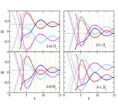
Figure 7: (Color online) Spectrum of Shiba states for a dimer with parallel orientation of the spins along the $z$ axis, within the sector $x^{2}-y^{2}$ for different strengths of the exchange interaction $J$ (in units of $J_{c}$) as a function of the distance between the impurities $r$ (in units of $k_{F}^{-1}$). $J_{c}=1/(\pi\nu S)$ is the critical coupling for the phase transition of a single impurity. The coherence length of the superconductor is $\xi_{0}=100/k_{F}$. The exact solution is plotted in solid lines, while dashed lines correspond to the spectrum calculated with the effective Hamiltonian. Dark (light) plots correspond to states polarized antiparallel (parallel) to the impurity. Blue and red correspond to $+$ and $-$ combinations. Dark and light dotted horizontal lines indicate the energies $E_{x^{2}-y^{2}}^{\pm}$ of the single impurities. The vertical lines indicate phase transitions.

We show now some results for the spectrum of a YSR dimer calculated by exactly calculating the subgap Green’s function, as explained in Section III, as well as from the solution of the effective Hamiltonian. In order to analyze the effect of the distance, we start by focusing on the channel $x^{2}-y^{2}$. Results for parallel spins oriented along the $z$-direction are shown in Fig. 7. The Fig. shows the spectrum as a function of the distance between impurities for four different values of $J$. It is convenient to notice that the configuration where the two impurities are far apart, the physics is expected to be similar to that of a single impurity. In the long-distance behavior of the dimer we can identify the asymptotic limit to the energies of the YSR states of a single impurity, $E_{x^{2}-y^{2}}^{\pm}$ given by Eq. (31). The latter are indicated in dotted lines in the Fig. For parallel spins, the interaction mediated by the substrate is only a hopping term in the framework of the effective Hamiltonian of Eq. (44),

$$H_{\rm eff,parallel}=\epsilon_{0}\left(c^{\dagger}_{1}c_{1}+c^{\dagger}_{2}c_{2}\right)+t\left(c^{\dagger}_{1}c_{2}+h.c\right).$$ (53)

This can be easily verified by evaluating the scalar products entering Eq. (48). Expressed in the operators ${\bf c}^{\dagger}=(c^{\dagger}_{1},c^{\dagger}_{2},c_{1},c_{2})$, the effective Hamiltonian matrix reads ${\cal H}_{\rm eff,parallel}=\epsilon_{0}\tau_{z}+ts_{x}\tau_{z}$, where $\tau_{z}$ is the $z$ Pauli matrix defined in the particle-hole degrees of freedom, while $s_{x}$ is the $x$ Pauli matrix for the impurity indices $1,\;2$. The eigenenergies are $E_{\pm,+}=|\epsilon_{0}\pm t|$ and $E_{\pm,-}=-|\epsilon_{0}\pm t|$. Here, the first index $\pm$ refers to bonding (+) and antibonding (-) combinations of the single impurity states, while the second corresponds to ${\rm s}=\pm$ as in Section III.

Hence, the hybridization leads to the formation of bonding and antibonding combinations, which are polarized antiparallel or parallel to the impurities. Focusing on the long-distance region of the plots and comparing the different panels, we can identify the transition to the bound state of the single impurity, as $J$ increases and overcomes the critical value $J_{c}$. Notice that states plotted in dark and light colors cross as $J>J_{c}$. We see that the agreement between the exact solution and the prediction of the effective Hamiltonian is excellent for distances $r>\lambda_{F}$. When the two impurities are very close ($r<\lambda_{F}$), only the exact solution is reliable. The physical picture of this regime can be understood in terms of a single impurity with an effective spin $S^{\rm eff}=2S$, which corresponds to $J_{c}^{\rm eff}=J_{c}/2$, as mentioned before. For this reason, even when the Shiba states of the single isolated impurity are not bound, they become bounded when the impurities are very close one another. For intermediate distances, many transitions may take place, depending on the value of the exchange interaction, which are indicated by vertical lines in the Fig. For the case of $J=0.7J_{c}$, shown in the upper left panel of the Fig., there are two phase transitions. Starting from the large-$r$ limit, there is a transition to a phase where the $+$ state is bound, while the $-$ remains unbounded. As $r$ decreases further, there is a transition to the short-distance phase, where both molecular states ($+$ and $-$) are bound. For $J=0.9J_{c}$, shown in the left bottom panel of the Fig., several phase transitions take place. Starting from the two unbound states in the long-distance regime, the $+$ and $-$ states alternate to get bound and unbound as $r$ decrease. We can observe a similar situation for $J=1.1J_{c}$ (upper right panel), but in this case the long-distance phase corresponds to the two molecular states bound. For even larger $J$, as in the case shown in the bottom right panel, the number of intermediate transitions decrease, and there is only a single phase with only one molecular bounded state. In all the cases shown in the figure, the short-distance regime ($r<\lambda_{F}$) correspond to two states bounded to an effective impurity with $S^{\rm eff}$. Following Ref. moca, , we can make contact to the Kondo effect taking place in a dimer of quantum spins. The regime with two bound states corresponds to maximum screening while the case of a single bound state corresponds to an orbital doublet and underscreened Kondo effect.

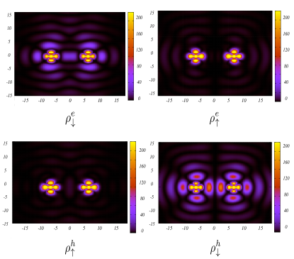
Figure 8: (Color online) Spectral function $\rho^{e,h}_{\sigma}(x,y,0)$ for the Shiba states within the channel $x^{2}-y^{2}$ for impurities with parallel spins separated in $r=10$, and exchange interaction $J=0.9J_{c}$. Both states correspond to the positive-energy region of the spectrum. The left (right) panels correspond to the state with highest (lowest) energy, which are bonding (antibonding) configurations. Other details are the same as in Fig. 7.

We now show the spectral densities defined in Eq. (38) of the YSR states of a dimer, for the particular cases of the spectra shown in the previous section. We have verified that the spectral density calculated with the eigenstates of the effective Hamiltonian, as defined in Eq. (49), reproduces the exact result for the distance between impurities shown in Fig. 8. The latter can be computed from the eigenstates of the effective Hamiltonian and the transformation of Eq. (III.3) and (III.3) with $\theta_{1}=\theta_{2}=\phi_{1}=\phi_{2}=0$. Fig. 8 corresponds to the dimer with parallel spins in the ${x^{2}-y^{2}}$ channel shown in Fig. 7. The spectral density provides information on the nature of the excited states. In fact, the spacial distribution enables the identification of a bonding or antibonding combination. In addition, as in the case of a single impurity, excitations with positive energy and dominant particle component with spin antiparallel to the impurity imply a ground state without bound states in that channel for that configuration. Instead, excitations with positive energy and dominant hole component with spin aligned with the impurity implies a ground state with a bound state in that configuration and channel. In the example of Fig. 8 we can identify the bonding (antibonding) configuration in the left (right) panels. The analysis of the components of the density of states resolved in spin and charge conjugation reveals that the ground state in the first case is unbounded, while it is bounded in the second one, in agreement with the analysis of the spectrum shown in Fig. 8. The substrate and the crystal field splitting strongly affects the shape of the maps for the spectral densities. As an example, we can compare with Fig. 1, which corresponds to the the bonding state with positive energy for the same parameters as Fig. 8. The only difference between the configurations of Figs. 1 and 8 is the orientation of the line connecting the two impurities relative to the axis of the crystal field. We see that the pattern of the spectral density differs. However, in both cases we can identify a bonding configuration.

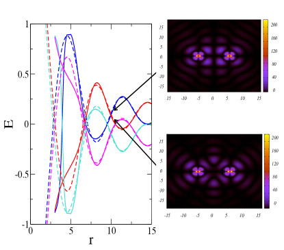
Figure 9: (Color online) Spectrum as a function of the distance and spectral function $\rho^{e}_{\sigma}(x,y,0)$ for selected Shiba states within the channel $xy$ for impurities with parallel spins separated in $r=10$. The hole components, $\rho^{e}_{\uparrow}(x,y,0)$, are fainter and they are not shown. The exchange interaction is $J=0.9J_{c}$. Other details are the same as in previous Figs.

The behavior of the spectrum and the spectral densities for the other channels is illustrated in Figs. 9, 10, 11 and 12. We can see that, although the asymptotic states in the limit of large distance between impurities are the same for all the channels, as a function of the distances there are a large number of crossings and the ordering of the states changes significantly. For the selected cases where the spectral densities are shown, we see that we can easily identify the bonding and antibonding configuration in the Figs. 9 and 10. In the case of Figs. 11 and 12 the spectral densities are fainter for the value $z=0$ chosen for the plots, as a consequence of the small projection of the $xz$ and $yz$ orbitals on this plane. In the cases shown, all the ground states are unbound, which is reflected by the dominant spectral density in the particle sector with spin antiparallel to the impurities. The results shown in Figs. 9 and 10 correspond to the dimer oriented in different directions with respect to the axis of the crystal field. Comparing the two figures, we see that the orientation does not have a major impact in the spectrum. However, it plays a role in the spacial distribution of the wave functions. In the orientation shown in Fig. 12 the two orbitals hybridize to form configurations of the type $d_{xz}\pm d_{yz}$ and the spectral density modifies accordingly. These details are a consequence of the type of substrate and the crystal field.

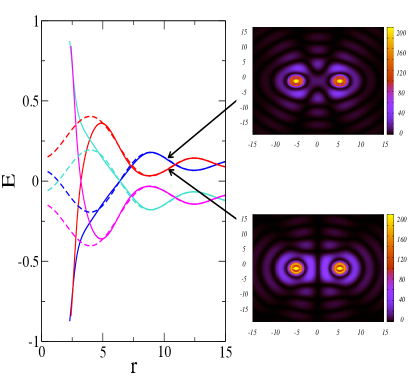
Figure 10: (Color online) Spectrum as a function of the distance and spectral function $\rho^{e}_{\uparrow}(x,y,0)$ for selected Shiba states within the channel $z^{2}$ for impurities with parallel spins separated in $r=10$. The exchange interaction is $J=0.9J_{c}$. The hole components, $\rho^{h}_{\uparrow}(x,y,0)$, are fainter and they are not shown. Other details are the same as in previous Figs.

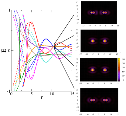
Figure 11: (Color online) Spectrum as a function of the distance and spectral function $\rho^{e}_{\uparrow}(x,y,0)$ for selected Shiba states within the degenerate channels $xz,\;yz$ for impurities with parallel spins separated in $r=10$. The exchange interaction is $J=0.9J_{c}$. Other details are the same as in previous Figs.

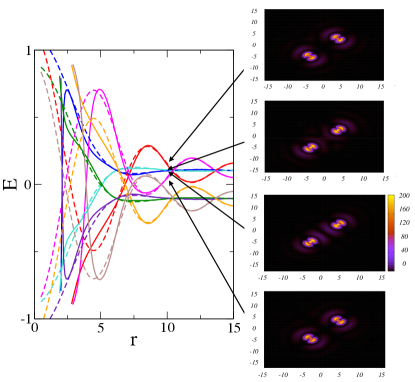
Figure 12: (Color online) Spectrum as a function of the distance and spectral function $\rho^{e}_{\uparrow}(x,y,0)$ for selected Shiba states within the degenerate channels $xz,\;yz$ for impurities with parallel spins separated in $r=10$. The exchange interaction is $J=0.9J_{c}$. The dimer is oriented forming an angle $\pi/4$ with respect to the $x$ axis of the crystal field. Other details are the same as in previous Figs.

IV.3 Dimer with tilted spins

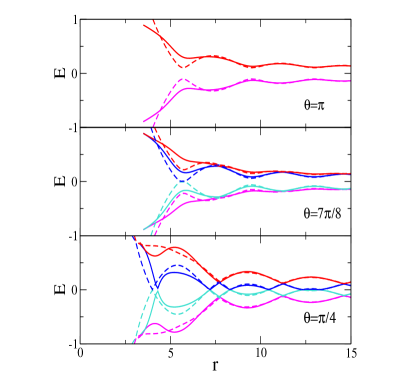
Figure 13: (Color online) Spectrum of Shiba states for a dimer with tilted magnetic moments $\theta_{1}=0,\theta_{2}=\theta$ with respect to the $z$ axis, and $J=0.9J_{c}$, as a function of the distance between the impurities $r$. Other details are the same as in Fig. 7.

When the spins of the impurities are tilted by an angle $\theta=\theta_{1}-\theta_{2}$, the midgap states not only hybridize but also become paired with an effective $p$-wave interaction. Hence, the ground state of the full system consists of the two unscreened impurities in the BCS condensate of the substrate plus the BCS state of the paired subgap states. This is illustrated in the sketches of Figs. 5 and 6. The Shiba states in this case correspond to excitations of the BCS state with $p$-wave pairing.

$$H_{\rm eff,\theta}=\epsilon_{0}\left(c^{\dagger}_{1}c_{1}+c^{\dagger}_{2}c_{2}\right)+t\;c^{\dagger}_{1}c_{2}+\Delta c^{\dagger}_{1}c^{\dagger}_{2}+h.c.$$ (54)

In Nambu language, this can be represented by the matrix ${\cal H}^{eff}_{\theta}=\epsilon_{0}\tau_{z}+ts_{x}\tau_{z}+\Delta s_{y}\tau_{y}$. The corresponding eigenenergies are

$$E_{\pm,\pm}=\pm\sqrt{\epsilon_{0}^{2}+t^{2}+\Delta^{2}\pm 2t\sqrt{\Delta^{2}+\epsilon_{0}^{2}}},$$ (55)

where, as before, the second label ${\rm s}=\pm$ indicates positive and negative energies and the first $\pm$ labels the two possible solutions in each case. The spectrum is always gapped for $|t|<\sqrt{\Delta^{2}+\epsilon_{0}^{2}}$. This is the case, in particular, for impurities with antiparallel magnetic moments ($\theta=\pi$), where It can be verified that the hopping term of Eq. (48) vanishes ($t=0$), while the pairing term is finite.

Example of the spectra for dimers of impurities with a relative angle $\theta$ between the magnetic moments are shown in Fig. 13 within the channel $d_{x^{2}-y^{2}}$. The upper panel corresponds to the antiparallel configuration. As before it is useful to start the analysis in the long-distance regime, where the inter-impurity effects are very small and we expect that the YSR states correspond to states that are basically the corresponding ones of the single impurity. As the impurities become closer, an hybridization takes place between $\downarrow$ quasiparticles localized at the impurity $1$ and $\uparrow$ quasiholes localized at the impurity $2$. The spectrum is always gapped in this case. Since the total spin $S_{z}=0$, each of these excited states have a doubly degeneracy. While the behavior of the dimer of parallel spins can be related to the Kondo effect of quantum spins, this is not the case of the antiparallel configuration. Other angles of the relative orientation of the magnetic moments of the dimer are shown in the other panels of the Fig. 13. The lower panel corresponds to a tilt closer to the parallel configuration of the impurities. The amplitude of the hopping, $|t|$, increases as $\theta$ decreases and is a function of the distance between the impurities. For some distances, the hopping overcomes the critical value $t_{c}=\sqrt{\Delta^{2}+\epsilon_{0}^{2}}$, for which the gap closes and level crossings at zero energy are observed in the spectrum. As before, this can be interpreted as a quantum phase transition where the parity of the ground state changes. The nature of the bound state is different from that of the fully polarized system. In fact, impurities with parallel magnetic moments the excitations and, in particular, the bound states, are simple bonding and antibonding combinations of the YSR states localized at the individual impurities. Instead, in the tilted case, the latter form a p-wave BCS state, which is degenerate with that of the substrate and the subgap excitations are the excitations of this state of p-wave pairs. When the dimer has a net polarization, these excitations disperse in bonding and antibonding combinations and eventually some of them can cross zero energy and get bounded to the net magnetic moment of the dimer.

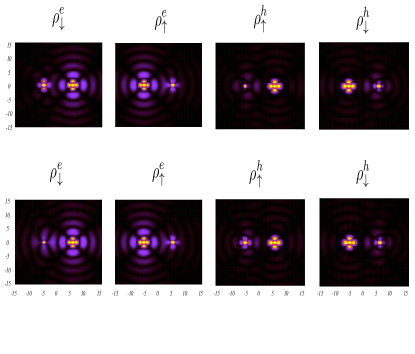
Figure 14: (Color online) Spectral function $\rho^{e,h}_{\sigma}(x,y,0)$ for the two Shiba states with positive energy within the channels $x^{2}-y^{2}$ for impurities with a tilt of $\theta=7\pi/8$ in the magnetic moments separated in $r=10$. Upper and lower panels corresond, respectively to highest and lowest energies. The exchange interaction is $J=0.9J_{c}$. Other details are the same as in previous figures.

We have shown results for a single channel, but similar results are obtained in the different channels and only the shape of the wave-function configuration change. In these figures, we have shown results obtained by exactly calculating the subgap Green’s function. In all the cases shown, we have compared with the spectral densities calculated with the effective Hamiltonian and we have verified that the agreement is excellent.

In Fig. 14 we illustrate the behavior of the spectral density of a dimer with magnetic moments forming an angle $\theta=7\pi/8$ in the orbital channel $d_{x^{2}-y^{2}}$. The total spectral density corresponding tho this configuration is shown in Fig. 15.

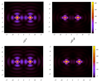
Figure 15: (Color online) Spectral function $\rho^{e,h}(x,y,0)=\sum_{\sigma}\rho^{e,h}_{\sigma}(x,y,0)$ for the two Shiba states with positive energy within the channels $x^{2}-y^{2}$ for impurities with a tilt of $\theta=7\pi/8$ in the magnetic moments separated in $r=10$. Other details are the same as in the previous figure.

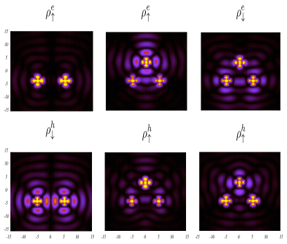
Figure 16: (Color online) Spectral function $\rho^{e,h}_{\sigma}(x,y,0)$ for the degenerate Shiba states with positive energy within the channels $x^{2}-y^{2}$ two impurities ferromagnetically aligned along the $z$ axis and a third impurity with antiparallel orientation with respect to the other two. The three impurities are separated by the same distance $r=10$, forming an equilateral triangle. The exchange interaction is $J=0.9J_{c}$. Left (right) configurations correspond to the state with lowest (highest) energy. The vanishing components are not shown. Other details are the same as in the previous figure.

IV.3.1 Trimer with magnetic frustration

We close with an illustration of the trimer configuration. In the case of three impurities, there are several possible scenarios, which depend on the orientations of the magnetic moments as well as on the spacial configuration of the cluster. We are not going to do an exhaustive analysis of the trimer, but just illustrate here how the previous techniques and analysis can be extended to study more complex clusters.

When the three impurities are ferromagnetically alined, the expected scenario is basically a generalization of the one discussed for the ferromagnetic dimer. The antiferromagnetic configuration is, however, frustrated in the present case. In what follows, we focus on such situation, which corresponds to two of the impurities with the magnetic moments ferromagnetically aligned and the third one antiferromagnetically oriented with respect to the other two. The effective Hamiltonian for impurities separated by $r>\lambda_{F}$ is

$$H_{\rm eff}^{\uparrow\uparrow\downarrow}=\epsilon_{0}\sum_{j=1}^{3}c^{\dagger}_{j}c_{j}+t_{12}c^{\dagger}_{1}c_{2}+\Delta_{23}c^{\dagger}_{2}c^{\dagger}_{3}+\Delta_{31}c^{\dagger}_{3}c^{\dagger}_{1}+H.c.,$$ (56)

which corresponds to a tight-binding hopping between the states localized at the two parallel impurities (labeled with $j=1,2$) and a p-wave pairing term between the latter and the states localized at the third one (labeled with $j=3$). For the case where the cluster is spatially organized forming an equilateral triangle with the parallel impurities placed on the $x$ axis and the antiparallel one on the $y$-axis, we can see that $\Delta_{23}=-\Delta_{31}=\Delta$. Then we can rewrite the effective Hamiltonian of Eq. (56), in terms of the bonding and antibonding combinations of states localized at $1$ and $2$, respectively, $c_{\pm}=\left(c_{1}\pm c_{2}\right)/\sqrt{2}$. The result is

$$H_{\rm eff}^{\uparrow\uparrow\downarrow}=\epsilon_{0}c^{\dagger}_{3}c_{3}+\sum_{j=\pm}E_{j}c^{\dagger}_{j}c_{j}+\sqrt{2}{\Delta}\left(c^{\dagger}_{+}c^{\dagger}_{3}+H.c.\right),$$ (57)

which corresponds to a pairing interaction between the third impurity and the bonding configuration of 1 and 2, while the antibonding configuration only couples the parallel impurities $j=1,2$. This implies that only the antibonding configuration can bound to screen the parallel impurities while the bonding will always form an effective BCS state with the localized states of the third impurity. The corresponding density of states for these excitations are shown in Fig. 16 focusing on the $d_{x^{2}-y^{2}}$ channel. For the parameters chosen, the lowest-energy state with positive energy has the spectral density shown in the left panels of Fig. 16 and corresponds to an excitation where the ground state is formed with the antibonding state bound to the parallel impurities. The other two states are the two excitations of the paired bonding state and the localized state at the third impurity. Since the total spin of the impurities is different from zero in this case, the excitations with $\uparrow$ and $\downarrow$ spins are not degenerate and their spectral densities are shown in the central and right panel of Fig. 16.

V Summary and conclusions

We have presented a systematic theoretical framework to analyze the spectrum and density of states of Yu-Shiba-Rusinov states of clusters of magnetic adatoms with multiple active orbitals and large magnetic moments in superconducting substrates. The treatment is based on the formulation of a multiorbital Kondo Hamiltonian considering the total spin of the impurity as a classical magnetic moment. We have defined an effective Green’s function to describe the subgap states, such that the poles of this function coincide with the poles of the $T$-matrix of the problem. Given this Green’s function, we can calculate the contribution of the subgap states with the local density of states and also define an effective Hamiltonian to describe clusters of diluted impurities.

We have analyzed the case of dimers in substrates with constant density of states assuming the effect of the crystal field in the Kondo model. We have analyzed different relative orientations of the magnetic moments and found an excellent agreement between the exact solution of the problem and the description based on the effective Hamiltonian. We have successfully described not only the spectrum but also the local density of states in the different orbital channels. We have briefly analyzed the case of a trimer.

For simplicity we focused on a simple substrate with s-wave superconductivity modeled by a BCS Hamiltonian expressed in the basis of plane waves. The present systematic approach to evaluate the subgap Green’s function can be also implemented in models for more realistic substrates, which include lattice effects, several bands and spin-orbit interaction. This method can be also useful to go beyond the BCS Hamiltonian model with a rigid gap and to calculate the correction to the local gap due to the presence of the impurity. Such correction was found to be relevant, in particular, for impurities localized at energies close to the onset of he quasiparticle continuum. meng1 ; meng2 In the present framework, the first correction to the bare gap due to the impurity can be calculated by solving the gap equation with the anomalous component of the Green’s function of Eq. (III.1), and the T-matrix evaluated by recourse to the subgap Green’s function as expressed in Eq. (21). We have verified that the latter approximation leads to an accurate description of the subgap spectrum and the density of states, not only for Shiba states deep in the gap but also in cases where their energies are close to the gap, hence it is reasonable to expect that it can be also useful to compute effects related to the gap renormalization.

VI Acknowledgements

The author thanks Felix von Oppen for interesting discussions, as well as A. A. Aligia and N. Lorente for stimulating comments. The author also thanks the hospitality of the Dahlem Center for Complex quantum Systems, Berlin under the support of the Alexander von Humboldt Stiftung, Germany. LA also acknowledges support from PIP-2015-CONICET, PICT-2017, PICT-2018, Argentina, and Simons-ICTP-Trieste associateship Argentina.

Appendix A Calculation of $F$

A.1 Single impurity

We start from the definition of the function in Eq. (19) and consider a constant density of states $\nu\simeq\sum_{\bf k}\delta(\xi-\xi_{\bf k})$. Then,

$$F(\omega)=\sum_{\bf k}G^{0}(\xi_{\bf k},\omega)=\int d\xi\sum_{\bf k}\delta(\xi-\xi_{\bf k})G^{0}(\xi,\omega)=\nu\int d\xi G^{0}(\xi,\omega).$$ (58)

The non-interacting Green function is

$$G^{0}(\xi,\omega)=\left[(\omega+i\eta)\tau_{0}-\xi\tau_{z}-\Delta\tau_{x}\right]^{-1}=\frac{1}{(\omega+i\eta)^{2}-\xi^{2}-\Delta^{2}}\left[(\omega+i\eta)\tau_{0}+\xi\tau_{z}+\Delta\tau_{x}\right].$$ (59)

Then

$$F(\omega)=-\nu\int d\xi\frac{1}{(\xi-i\overline{\xi})(\xi+i\overline{\xi})}\left[\omega\tau_{0}+\Delta\tau_{x}\right]=-\frac{\nu\pi}{\sqrt{\Delta^{2}-\omega^{2}}}\sigma_{0}\left[\omega\tau_{0}+\Delta\tau_{x}\right],\;\,\;\;\;\;\;\;\;\;|\omega|<\Delta,$$ (60)

with $\overline{\xi}=\sqrt{\Delta^{2}-\omega^{2}}$.

A.2 Two impurities

The diagonal components of the function defined in Eq. (IV.2) are $F_{\mu,\mu^{\prime}}^{1,1}(\omega)=F_{\mu,\mu^{\prime}}^{2,2}(\omega)=\delta_{\mu,\mu^{\prime}}F(\omega)$. Here, we calculate the off-diagonal components. In the case of a strong crystal-field splitting, it is reasonable to assume that the matrix elements of the $F$ matrix are diagonal in the index $\mu$. In order to calculate the off-diagonal elements of the matrix $F$ we must project the real-space components of the function $e^{i{\bf k}\cdot({\bf r}_{1}-{\bf r}_{2})}$ in the same axis as the orbitals. Therefore, the off-diagonal matrix element reads

$$F_{\mu,\mu^{\prime}}^{1,2}(\omega) = (4\pi)^{2}L^{3}\sum_{l,m}(i)^{l}Y^{m}_{l}(\hat{r}_{12})\int\frac{dk}{(2\pi)^{3}}k^{2}j_{l}\left(kr_{12}\right)G^{0}(k,\omega)\int d\Omega_{k}Y^{m}_{l}(\Omega_{k})f_{\mu}(\Omega_{k})^{*}f_{\mu^{\prime}}(\Omega_{k})$$

$$= 4\pi\nu\sum_{l}(i)^{l}\;{\cal C}_{\mu,\mu^{\prime}}(l)\int d\xi j_{l}\left(\left(\frac{\xi}{{\rm v}_{F}}+k_{F}\right)r_{12}\right)G^{0}(\xi,\omega)=-4\pi\nu\sum_{l}(i)^{l}\;{\cal C}_{\mu,\mu^{\prime}}(l)\left[\left(\omega\tau_{0}+\Delta\tau_{x}\right)I^{(l)}_{1}(r_{12},\omega)+\tau_{z}I^{(l)}_{2}(r_{12},\omega)\right],$$

with $r_{12}=|{\bf r}_{1}-{\bf r}_{2}|$ and using the following definition of the integrals of Bessel functions

$$I^{(l)}_{j}(r,\omega)=\int d\xi j_{l}\left((\frac{\xi}{v_{F}}+k_{F})r\right)\frac{\xi^{j-1}}{\xi^{2}+\Delta^{2}-\omega^{2}},\;\;\;\;\;j=1,2.$$ (62)

The calculation of these integrals is detailed in Appendix (C) for the cases $l=0,2,4$. Notice that they have the following structure

$$I^{(l)}_{j}=\lambda_{j}(r,\omega)\kappa^{(l)}_{j}(k_{F}r),$$ (63)

where the functions $\lambda_{j}(r,\omega)$ are defined in Eq. (75) and the functions $\kappa$ are defined in Eqs. (74), (C.0.2) and (C.0.3), respectively. The coefficients entering the above expression are

$${\cal C}_{z^{2}}(l) = \left(\delta_{l,0}+\delta_{l.2}+\delta_{l,4}\right)C_{2,2,l}^{0,0,0}Y^{0}_{l}(\hat{r}_{12}),$$

$${\cal C}_{x^{2}-y^{2}}(l) = \frac{1}{2}\left[\left(C_{2,2,4}^{2,2,-4}Y^{-4}_{4}(\hat{r}_{12})+C_{2,2,4}^{-2,-2,4}Y^{4}_{4}(\hat{r}_{12})\right)\delta_{l,4}+2\left(\delta_{l,0}+\delta_{l.2}+\delta_{l,4}\right)C_{2,2,l}^{-2,2,0}Y^{0}_{l}(\hat{r}_{12})\right],$$

$${\cal C}_{xy}(l) = \frac{1}{2}\left[-\left(C_{2,2,4}^{-2,-2,4}Y^{4}_{4}(\hat{r}_{12})+C_{2,2,4}^{2,2,-4}Y^{-4}_{4}(\hat{r}_{12})\right)\delta_{l,4}+2\left(\delta_{l,0}+\delta_{l.2}+\delta_{l,4}\right)C_{2,2,l}^{-2,2,0}Y^{0}_{l}(\hat{r}_{12})\right],$$

$${\cal C}_{xz}(l) = \frac{1}{2}\left[-\left(C_{2,2,l}^{-1,-1,2}Y^{2}_{l}(\hat{r}_{12})+C_{2,2,l}^{1,1,-2}Y^{-2}_{l}(\hat{r}_{12})\right)\left(\delta_{l.2}+\delta_{l,4}\right)+2\left(\delta_{l,0}+\delta_{l.2}+\delta_{l,4}\right)C_{2,2,l}^{-1,1,0}Y^{0}_{l}(\hat{r}_{12})\right],$$

$${\cal C}_{yz}(l) = \frac{1}{2}\left[\left(C_{2,2,l}^{-1,-1,2}Y^{2}_{l}(\hat{r}_{12})+C_{2,2,l}^{1,1,-2}Y^{-2}_{l}(\hat{r}_{12})\right)\left(\delta_{l.2}+\delta_{l,4}\right)+2\left(\delta_{l,0}+\delta_{l.2}+\delta_{l,4}\right)C_{2,2,l}^{-1,1,0}Y^{0}_{l}(\hat{r}_{12})\right],$$

$${\cal C}_{xz,yz}(l) = -\frac{i}{2}\left[\left(C_{2,2,l}^{-1,-1,2}Y^{2}_{l}(\hat{r}_{12})-C_{2,2,l}^{1,1,-2}Y^{-2}_{l}(\hat{r}_{12})\right)\left(\delta_{l.2}+\delta_{l,4}\right)\right],$$

$${\cal C}_{xy,xz}(l) = -\frac{i}{2}\left[\left(C_{4,2,2}^{3,-2,-1}Y^{3}_{4}(\hat{r}_{12})+C_{4,2,2}^{-3,2,1}Y^{-3}_{4}(\hat{r}_{12})\right)\delta_{l,4}-\left(Y^{-1}_{l}(\hat{r}_{12})C_{l,2,2}^{-1,2,-1}+Y^{1}_{l}(\hat{r}_{12})C_{l,2,2}^{1,-2,1}\right)\left(\delta_{l.2}+\delta_{l,4}\right)\right],$$

$${\cal C}_{xy,yz}(l) = -\frac{1}{2}\left[\left(C_{4,2,2}^{3,-2,-1}Y^{3}_{4}(\hat{r}_{12})-C_{4,2,2}^{-3,2,1}Y^{-3}_{4}(\hat{r}_{12})\right)\delta_{l,4}-\left(Y^{-1}_{l}(\hat{r}_{12})C_{l,2,2}^{1,-2,1}-Y^{1}_{l}(\hat{r}_{12})C_{l,2,2}^{-1,2,-1}\right)\left(\delta_{l.2}+\delta_{l,4}\right)\right]$$ (64)

The latter depend on integrals of products of three spherical harmonics, which can be expressed in terms of the $3j$ Wigner coefficient as follows

$$C_{l_{1},l_{2},l_{3}}^{m_{1},m_{2},m_{3}}=\int d\Omega_{k}Y^{m_{1}}_{l_{1}}(\Omega_{k})Y_{l_{2}}^{m_{2}}(\Omega_{k})^{*}Y_{l_{3}}^{m_{3}}(\Omega_{k})Y_{l_{3}}^{m_{3}}(\hat{r}_{12})=\sqrt{\frac{(2l_{1}+1)(2l_{2}+1)(2l_{3}+1)}{4\pi}}\left(\begin{array}[]{ccc}l_{1}l_{2}l_{3}\\ m_{1}m_{2}m_{3}\end{array}\right)\left(\begin{array}[]{ccc}l_{1}l_{2}l_{3}\\ 000\end{array}\right)Y_{l_{3}}^{m_{3}}(\hat{r}_{12}).$$ (65)

In our case, we have: $l_{1}=l_{2}=2$. The sum over $l,m$ is restricted to the terms satisfying the selection rules of the $3j$ symbol, namely $m_{1}+m_{2}+m_{3}=0$ and $l=0,2,4$.

We present bellow a table with the values of the different coefficients $C_{l_{1},l_{2},l_{3}}^{m_{1},m_{2},m_{3}}$ entering (A.2)

$C_{2,2,0}^{0,0,0}$	$C_{2,2,0}^{-1,1,0}$	$C_{2,2,0}^{-2,2,0}$
$\sqrt{\frac{1}{4\pi}}$	$-\sqrt{\frac{1}{4\pi}}$	$\sqrt{\frac{1}{4\pi}}$

$C_{2,2,2}^{0,0,0}$	$C_{2,2,2}^{-2,2,0}$	$C_{2,2,2}^{-1,-1,2}$	$C_{2,2,2}^{1,1,-2}$	$C_{2,2,2}^{-1,1,0}$	$C_{2,2,2}^{-1,2,-1}$
$\frac{1}{7}\sqrt{\frac{5}{\pi}}$	$-\frac{1}{7}\sqrt{\frac{5}{4\pi}}$	$\frac{1}{7}\sqrt{\frac{15}{2\pi}}$	$\frac{1}{7}\sqrt{\frac{15}{2\pi}}$	$-\frac{1}{4}\sqrt{\frac{5}{\pi}}$	$\frac{1}{14}\sqrt{\frac{30}{\pi}}$

$C_{2,2,4}^{0,0,0}$	$C_{2,2,4}^{2,2,-4}$	$C_{2,2,4}^{-2,-2,4}$	$C_{2,2,4}^{-2,2,0}$	$C_{2,2,4}^{-1,-1,2}$	$C_{2,2,4}^{1,1,-2}$	$C_{2,2,4}^{-1,1,0}$	$C_{4,2,2}^{-1,2,-1}$	$C_{4,2,2}^{3,-2,-1}$
$\frac{3}{7}\sqrt{\frac{1}{\pi}}$	$5\sqrt{\frac{1}{70\pi}}$	$5\sqrt{\frac{1}{70\pi}}$	$\frac{1}{7}\sqrt{\frac{1}{2\pi}}$	$\frac{1}{7}\sqrt{\frac{10}{\pi}}$	$\frac{1}{7}\sqrt{\frac{10}{\pi}}$	$\frac{2}{7}\sqrt{\frac{1}{\pi}}$	$-\frac{5}{14}\sqrt{\frac{1}{5\pi}}$	$-\frac{5}{2}\sqrt{\frac{1}{35\pi}}$

Appendix B Calculation of the matrices $\gamma_{\mu}$

Following a similar procedure as the one followed to calculate $F$, we have for plane waves

$$\gamma_{\mu}({\bf r},\omega) = \sum_{\bf k}\sum_{l^{\prime},m^{\prime}}(i)^{l^{\prime}}j_{l^{\prime}}(kr)Y_{l^{\prime}}^{m^{\prime}}(\hat{r})Y_{l^{\prime}}^{m^{\prime}}(\hat{k})f_{\mu}(\hat{k})^{*}G^{0}({\bf k},\omega)\simeq-4\pi\nu\int d\xi j_{2}\left(\frac{\xi}{{\rm v}_{F}}+k_{F}r\right)G^{0}(\xi,\omega)f_{\mu}(\hat{r})$$ (66)

$$= 4\pi\nu\left[\left(\omega\tau_{0}+\Delta\tau_{x}\right)I^{(2)}_{1}(r,\omega)+\tau_{z}I^{(2)}_{2}(r,\omega)\right]f_{\mu}(\hat{r}).$$ (67)

Notice that the asymptotic behavior is dominated by the terms $\propto 1/(k_{F}r)$ in the 3D case and as $1/\sqrt{k_{F}r}$ in the 2D one.

Appendix C Evaluation of integrals $I^{(l)}_{1}(r,\omega)$ and $I^{(l)}_{2}(r,\omega)$

We present the evaluation of integrals defined in Eq. (62) for the cases $l=0,2,4$. The corresponding Bessel functions are

$$j_{0}(u)=\frac{\sin u}{u},\;\;\;\;\;\;\;\;\;j_{2}(u)=\frac{\sin u}{u}\left[\frac{3}{u^{2}}-1\right]-\frac{3\cos u}{u^{2}},\;\;\;\;\;\;\;\;\;j_{4}(u)=\frac{\sin u}{u}\left[\frac{105}{u^{4}}-\frac{45}{u^{2}}+1\right]+\cos u\left[\frac{10}{u^{2}}-\frac{105}{u^{4}}\right],$$ (68)

with $u=\left(\xi/v_{F}+k_{F}\right)r$.

C.0.1 l=0

The integrals we have to evaluate can be expressed as follows

$$I^{(0)}_{j}=\frac{r}{v_{F}}\int du\frac{\sin u\left[v_{F}(u/r-k_{F})\right]^{j-1}}{(u-u_{+})(u-u_{-})u},$$ (69)

with

$$u_{\pm}=k_{F}r\pm ir\sqrt{\Delta^{2}-\omega^{2}}/v_{F}.$$ (70)

We proceed as follows

$$I^{(0)}_{1}=\frac{r}{v_{F}}\frac{1}{2i}\left[\int_{C_{1}}du\frac{e^{iu}}{(u+i\eta)(u-u_{+})(u-u_{-})}-\int_{C_{2}}du\frac{e^{-iu}}{(u-i\eta)(u-u_{+})(u-u_{-})}\right],$$ (71)

where $C_{1}\;(C_{2})$ are complex contours that runs along the real axis and close in semicircles with radius $R\rightarrow\infty$ in the upper (lower) semiplane. The result from Cauchy theorem is

$$I^{(0)}_{1}=\frac{\pi r}{v_{F}}\left[\frac{e^{iu_{+}}}{(u_{+}+i\eta)(u_{+}-u_{-})}+\frac{e^{-iu_{-}}}{(u_{-}-i\eta)(u_{-}-u_{+})}\right]=\frac{\pi}{\sqrt{\Delta^{2}-\omega^{2}}}\frac{e^{-\frac{r}{v_{F}}\sqrt{\Delta^{2}-\omega^{2}}}}{(k_{F}r)^{2}+(\Delta^{2}-\omega^{2})(r/v_{F})^{2}}\left(k_{F}r\sin k_{F}r-\frac{r}{v_{F}}\sqrt{\Delta^{2}-\omega^{2}}\right).$$ (72)

We proceed similarly with the other integral. The result is

$$I^{(0)}_{j}\simeq\lambda_{j}(r,\omega)\kappa^{(0)}_{j}(k_{F}r),\;\;\;\;\;\;\;\ r<\xi_{0},$$ (73)

where $\xi_{0}=v_{F}/\Delta$ is the coherence length of the superconductor. We have defined

$$\kappa^{(0)}_{1}(k_{F}r)=\frac{\sin k_{F}r}{k_{F}r},\;\;\;\;\;\;\;\kappa^{(0)}_{2}(k_{F}r)=\frac{\cos k_{F}r}{(k_{F}r)}.$$ (74)

and

$$\lambda_{1}(r,\omega)=\frac{\pi}{\sqrt{\Delta^{2}-\omega^{2}}}e^{-\sqrt{1-\left(\frac{\omega}{\Delta}\right)^{2}}\frac{r}{\xi_{0}}},\;\;\;\;\;\;\;\;\;\lambda_{2}(r,\omega)=\pi e^{-\sqrt{1-\left(\frac{\omega}{\Delta}\right)^{2}}\frac{r}{\xi_{0}}}.$$ (75)

C.0.2 l=2

We express the integrals for $j=1,2$ as $I^{(2)}_{1}(r,\omega)=I^{(2)}_{1,1}+I^{(2)}_{1,2}+I^{(2)}_{1,3}$, and $I^{(2)}_{2}(\omega)=I^{(2)}_{2,1}+I^{(2)}_{2,2}+I^{(2)}_{2,3}$ being

$$I^{(2)}_{j,1} = \frac{r}{v_{F}}\mbox{PV}\int du\frac{3\sin u\left[v_{F}(u/r-k_{F})\right]^{j-1}}{(u-u_{+})(u-u_{-})u^{3}},$$

$$I^{(2)}_{j,2} = -\frac{r}{v_{F}}\int du\frac{\sin u\left[v_{F}(u/r-k_{F})\right]^{j-1}}{(u-u_{+})(u-u_{-})u},$$

$$I^{(2)}_{j,3} = -\frac{r}{v_{F}}\mbox{PV}\int du\frac{3\cos u\left[v_{F}(u/r-k_{F})\right]^{j-1}}{(u-u_{+})(u-u_{-})u^{2}},$$ (76)

with $u_{\pm}$ defined in Eq. (70). We proceed as in the case with $l=0$. The results are

$$I^{(2)}_{j}\simeq\lambda_{j}(r,\omega)\kappa^{(2)}_{j}(k_{F}r),\;\;\;\;\;\;\;\;\;\;\;\;\;\;\;\;\;\;\;\;\kappa^{(2)}_{j}(k_{F}r)=\sum_{i=1}^{3}\kappa^{(2)}_{j,i}(k_{F}r)$$ (77)

with

$$\kappa^{(2)}_{1,1}(k_{F}r) = 3\frac{\sin k_{F}r}{(k_{F}r)^{3}},\;\;\;\;\;\;\;\kappa^{(2)}_{1,2}(k_{F}r)=-\frac{\sin k_{F}r}{k_{F}r},\;\;\;\;\;\;\;\kappa^{(2)}_{1,3}(k_{F}r)=-3\frac{\cos k_{F}r}{(k_{F}r)^{2}},$$

$$\kappa^{(2)}_{2,1}(k_{F}r) = 3\frac{\cos k_{F}r}{(k_{F}r)^{3}},\;\;\;\;\;\;\;\;\;\kappa^{(2)}_{2,2}(k_{F}r)=-\frac{\cos k_{F}r}{(k_{F}r)},\;\;\;\;\;\;\;\;\;\kappa^{(2)}_{2,3}(k_{F}r)=3\frac{\sin k_{F}r}{(k_{F}r)^{2}}.$$ (78)

The functions $\lambda_{1,2}$ are defined in Eq. (75).

C.0.3 l=4

We proceed as in the previous case and split the integrals as $I^{(4)}_{j}(r,\omega)=\sum_{i=1}^{5}I^{(4)}_{j,i},\;j=1,2$, being

$$I^{(4)}_{j,1} = 105\frac{r}{v_{F}}\mbox{PV}\int du\frac{\left[v_{F}(u/r-k_{F})\right]^{j-1}\sin u}{(u-u_{+})(u-u_{-})u^{5}},$$

$$I^{(4)}_{j,2} = -45\frac{r}{v_{F}}\mbox{PV}\int du\frac{\sin u\left[v_{F}(u/r-k_{F})\right]^{j-1}}{(u-u_{+})(u-u_{-})u^{3}},$$

$$I^{(4)}_{j,3} = \frac{r}{v_{F}}\mbox{PV}\int du\frac{\sin u\left[v_{F}(u/r-k_{F})\right]^{j-1}}{(u-u_{+})(u-u_{-})u},$$

$$I^{(4)}_{j,4} = 10\frac{r}{v_{F}}\mbox{PV}\int du\frac{\cos u\left[v_{F}(u/r-k_{F})\right]^{j-1}}{(u-u_{+})(u-u_{-})u^{2}},$$

$$I^{(4)}_{j,5} = -105\frac{r}{v_{F}}\mbox{PV}\int du\frac{\cos u\left[v_{F}(u/r-k_{F})\right]^{j-1}}{(u-u_{+})(u-u_{-})u^{4}}.$$ (79)

The results are

$$I^{(4)}_{j}=\lambda_{j}(r,\omega)\kappa^{(4)}_{j}(k_{F}r),\;\;\;\;\;\;\;\;\;\;\;\;\;\;\;\;\;\;\;\;\kappa^{(4)}_{j}(k_{F}r)=\sum_{i=1}^{5}\kappa^{(4)}_{j,i}(k_{F}r),$$ (80)

with

$$\kappa^{(4)}_{1,1}(k_{F}r) = 105\frac{\sin k_{F}r}{(k_{F}r)^{5}},\;\;\;\kappa^{(4)}_{1,2}(k_{F}r)=-45\frac{\sin k_{F}r}{(k_{F}r)^{3}},\;\;\;\kappa^{(4)}_{1,3}(k_{F}r)=\frac{\sin k_{F}r}{(k_{F}r)},\;\;\;\kappa^{(4)}_{1,4}(k_{F}r)=10\frac{\cos k_{F}r}{(k_{F}r)^{2}},\;\;\;\kappa^{(4)}_{1,5}(k_{F}r)=-105\frac{\cos k_{F}r}{(k_{F}r)^{4}},$$

$$\kappa^{(4)}_{2,1}(k_{F}r) = 105\frac{\cos k_{F}r}{(k_{F}r)^{5}},\;\;\;\kappa^{(4)}_{2,2}(k_{F}r)=-45\frac{\cos k_{F}r}{(k_{F}r)^{3}},\;\;\;\kappa^{(4)}_{2,3}(k_{F}r)=\frac{\cos k_{F}r}{(k_{F}r)},\;\;\;\kappa^{(4)}_{2,4}(k_{F}r)=-10\frac{\sin k_{F}r}{(k_{F}r)^{2}},\;\;\;\kappa^{(4)}_{2,5}(k_{F}r)=105\frac{\sin k_{F}r}{(k_{F}r)^{4}},$$

References

- (1) A. V. Balatsky, I. Vekhter, and J-X Zhu, Impurity-induced states in conventional and unconventional superconductors, Rev. Mod. Phys. 78, 373 (2006).
- (2) L. Yu, Bound state in superconductors with paramagnetic impurities, Acta Phys. Sin. 21, 75 (1965).
- (3) H. Shiba, Classical Spins in Superconductors, Prog. Theor. Phys. 40, 435 (1968).
- (4) A. I. Rusinov, On the theory of gapless superconductivity containing paramagnetic impurities, Sov. J. Exp. Theor. Phys. 29, 1101 (1969).
- (5) B. W. Heinrich, J. I. Pascual, and K. J. Franke, Single magnetic adsorbates on s-wave superconductors, Prog. Surf. Sci. 93, 1 (2018), references therein.
- (6) R. Zitko, J. S. Lim, Rosa López, and Ramón Aguado, Shiba states and zero-bias anomalies in the hybrid normal-superconductor Anderson model, Phys. Rev B 91, 045441 (2015).
- (7) R. Zitko, Spectral properties of Shiba subgap states at finite temperatures, Phys. Rev. B 93, 195125 (2016).
- (8) R. S. Deacon, Y. Tanaka, A. Oiwa, R. Sakano, K. Yoshida, K. Shibata, K. Hirakawa, and S. Tarucha, Tunneling Spectroscopy of Andreev Energy Levels in a Quantum Dot Coupled to a Superconductor, Phys. Rev. Lett. 104, 076805 (2010).
- (9) E. J. Lee, X. Jiang, M. Houzet, R. Aguado, C. M. Lieber, and S. De Franceschi, Spin-resolved Andreev levels and parity crossings in hybrid superconductor?semiconductor nanostructures, Nat. Nano 9, 79 (2014).
- (10) S. Nadj-Perge, I.K. Drozdov, B.A. Bernevig, and A. Yazdani, Proposal for realizing Majorana fermions in chains of magnetic atoms on a superconductor, Phys. Rev. B 88, 020407(R) (2013).
- (11) S. Nadj-Perge, I. K. Drozdov, B. A. Bernevig, and A. Yazdani, Observation of Majorana fermions in ferromagnetic atomic chains on a superconductor, Science 346, 602 (2014).
- (12) J. Klinovaja, P. Stano, A. Yazdani, and Daniel Loss, Topological Superconductivity and Majorana Fermions in RKKY Systems Phys. Rev. Lett. 111, 186805 (2013).
- (13) B. Braunecker and P. Simon,Interplay between Classical Magnetic Moments and Superconductivity in Quantum One-Dimensional Conductors: Toward a Self-Sustained Topological Majorana Phase Phys. Rev. Lett. 111, 147202 (2013)
- (14) G. C. Ménard, S. Guissart, C. Brun, S. Pons, V. S. Stolyarov, F. Debontridder, M. V. Leclerc, E. Janod, L. Cario, D. Roditchev, P. Simon, and T. Cren Coherent long-range magnetic bound states in a superconductor, Nature Phys. 11, 1013 (2015).
- (15) F. Pientka, L. I. Glazman, and F. von Oppen, Topological superconducting phase in helical Shiba chains, Phys. Rev. B 88, 180505 (2014)
- (16) C. Mier, J. Hwang, J. Kim, Y. Bae, F. Nabeshima, Y. Imai, A. Maeda, N. Lorente, A. Heinrich, D-J. Choi, Atomic Manipulation of In-gap States on the -Bi2Pd Superconductor, arXiv:2104.06171
- (17) S. Park, V. Barrena, S. Mañas-Valero, J. J. Baldovi, A. Fente, E. Herrera, F. Mompeán, M. Garcia-Hernandez, A. Rubio, E. Coronado, A. Levy Yeyati, H. Suderow, Coherent coupling between vortex bound states and magnetic impurities in 2D layered superconductors, arXiv:2103.04164
- (18) F. von Oppen and K. J. Franke, Yu-Shiba-Rusinov states in real metals, Phys. Rev. B 103, 205424 (2021)
- (19) C. P. Moca, E. Demler, B. Jankó, and G. Zaránd, Spin-resolved spectra of Shiba multiplets from Mn impurities in , Phys. Rev. 77, 174517 (2008)
- (20) M. Ruby, Y. Peng, F. von Oppen, K. Franke, Orbital Picture of Yu-Shiba-Rusinov Multiplets, Phys. Rev. Lett. 117, 186801 (2016)
- (21) D-J. Choi, C. Rubio-Verdú, J. de Bruijckere, M. M. Ugeda, N. Lorente and J. I. Pascual, Mapping the orbital structure of impurity bound states in a superconductor Nature Comm. 8, 15175 (2017)
- (22) T. A. Costi, L. Bergqvist, A. Weichselbaum, J. von Delft, T. Micklitz, A. Rosch, P. Mavropoulos, P. H. Dederichs, F. Mallet, L. Saminadayar, C. Bauerle, Kondo decoherence: finding the right spin model for iron impurities in gold and silver, Phys. Rev. Lett. 102, 056802 (2009)
- (23) P. S. Cornaglia, P. Roura Bas, A. A. Aligia and C. A. Balseiro, Quantum transport through a stretched spin-1 molecule, Europhys. Lett. 93, 4 (2011).
- (24) D. B. Karki, Christophe Mora, Jan von Delft, Mikhail N. Kiselev, Two-color Fermi liquid theory for transport through a multilevel Kondo impurity, Phys. Rev. B 97, 195403 (2018).
- (25) N. Roch, S. Florens, T. A. Costi, W. Wernsdorfer, and F. Balestro, Observation of the Underscreened Kondo Effect in a Molecular Transistor, Phys. Rev. Lett. 103, 197202 (2009)
- (26) J. J. Parks, A. R. Champagne, T. A. Costi, W. W. Shum, A. N. Pasupathy, E. Neuscamman, S. Flores-Torres, P. S. Cornaglia, A. A. Aligia, C. A. Balseiro, G. K.-L. Chan, H. D. Abruña2, D. C. Ralph, Mechanical Control of Spin States in Spin-1 Molecules and the Underscreened Kondo Effect, Science 328, 1370 (2010).
- (27) M.E.Flatté and J.M.Byers, Local electronic structure of defects in superconductors, Phys.Rev.B 56,11213 (1997).
- (28) N. Y. Yao,C. P. Moca, I. Weymann, J. D. Sau, M. D. Lukin, E. A. Demler, and G. Zaránd, Phase diagram and excitations of a Shiba molecule, Phys. Rev. B 90, 241108 (R) (2014).
- (29) S. Koerber, B. Trauzettel, and O. Kashuba Delocalized Yu-Shiba-Rusinov states in magnetic clusters at superconducting surfaces Phys. Rev. B 97, 184503 (2018)
- (30) A. A. Aligia, Effective Kondo Model for a Trimer on a Metallic Surface, Phys. Rev. Lett. 96, 096804 (2006)
- (31) G. O. Steffensen, J. C. Estrada Saldaña, A. Vekris, P. Krogstrup, K. Grove-Rasmussen, J. Nygard, A. Levy Yeyati, and J. Paaske, Direct Transport between Superconducting Subgap States in a Double Quantum Dot, arXiv:2105.06815.
- (32) S. Hoffman, J. Klinovaja, T. Meng, and D. Loss, Impurity Induced Quantum Phase Transitions and Magnetic Order in Conventional Superconductors: Competition between Bound and Quasiparticle states, Phys. Rev. B 92, 125422 (2015).
- (33) T. Meng, J. Klinovaja, S. Hoffman, P. Simon, and D. Loss, Superconducting Gap Renormalization around two Magnetic Impurities: From Shiba to Andreev Bound States, Phys. Rev. B 92, 064503 (2015)
- (34) D-J. Choi, C. García Fernández, E. Herrera, C. Rubio-Verdú, M. M. Ugeda, I. Guillamón, H. Suderow, J. I. Pascual, N. Lorente, Probing magnetic interactions between Cr adatoms on the -Bi2Pd superconductor, Phys. Rev. Lett. 120, 167001 (2018)
- (35) M. Ruby, B. W. Heinrich, Y. Peng, F. von Oppen, K. J. Franke, Wave-function hybridization in Yu-Shiba-Rusinov dimers, Phys. Rev. Lett. 120, 156803 (2018)
- (36) Hao Ding, Yuwen Hu, Mallika T. Randeria, Silas Hoffman, Oindrila Deb, Jelena Klinovaja Daniel Loss, and Ali Yazdani, Tuning interactions between spins in a superconductor, Proc. Natl. Acad. Sci. USA 118, 14 (2021)
- (37) P. Nozieres and A. Blandin, Kondo effect in real metals, J. Phys. Paris 41, 193 (1980).
- (38) A.M. Tsvelick and P. B. Wiegmann, Exact results in the theory of magnetic alloys, Adv. Phys. 32, 453 (1983).
- (39) A. Y. Kitaev, Physics-Uspekhi 44, 131 (2001).